A New Coefficient of Correlation

Abstract

Abstract–Is it possible to define a coefficient of correlation which is (a) as simple as the classical coefficients like Pearson’s correlation or Spearman’s correlation, and yet (b) consistently estimates some simple and interpretable measure of the degree of dependence between the variables, which is 0 if and only if the variables are independent and 1 if and only if one is a measurable function of the other, and (c) has a simple asymptotic theory under the hypothesis of independence, like the classical coefficients? This article answers this question in the affirmative, by producing such a coefficient. No assumptions are needed on the distributions of the variables. There are several coefficients in the literature that converge to 0 if and only if the variables are independent, but none that satisfy any of the other properties mentioned above. Supplementary materials for this article are available online.

KEYWORDS:

• Correlation
• Independence
• Measure of association

1 Introduction

The three most popular classical measures of statistical association are Pearson’s correlation coefficient, Spearman’s ρ, and Kendall’s τ. These coefficients are very powerful for detecting linear or monotone associations, and they have well-developed asymptotic theories for calculating p-values. However, the big problem is that they are not effective for detecting associations that are not monotonic, even in the complete absence of noise.

There have been many proposals to address this deficiency of the classical coefficients (Josse and Holmes 2016), such as the maximal correlation coefficient (Hirschfeld 1935; Gebelein 1941; Rényi 1959; Breiman and Friedman 1985), various coefficients based on joint cumulative distribution functions and ranks (Hoeffding 1948; Blum, Kiefer, and Rosenblatt 1961; Yanagimoto 1970; Puri and Sen 1971; Rosenblatt 1975; Csörgő 1985; Romano 1988; Bergsma and Dassios 2014; Nandy, Weihs, and Drton 2016; Weihs, Drton, and Leung 2016; Han, Chen, and Liu 2017; Wang, Jiang, and Liu 2017; Drton, Han, and Shi 2018; Gamboa, Klein, and Lagnoux 2018; Weihs, Drton, and Meinshausen 2018; Deb and Sen 2019), kernel-based methods (Gretton et al. 2005, 2008; Sen and Sen 2014; Pfister et al. 2018; Zhang et al. 2018), information theoretic coefficients (Linfoot 1957; Kraskov, Stogbauer, and Grassberger 2004; Reshef et al. 2011), coefficients based on copulas (Sklar 1959; Schweizer and Wolff 1981; Dette, Siburg, and Stoimenov 2013; Lopez-Paz, Hennig, and Schölkopf 2013; Zhang 2019), and coefficients based on pairwise distances (Friedman and Rafsky 1983; Székely, Rizzo, and Bakirov 2007; Székely and Rizzo 2009; Heller, Heller, and Gorfine 2013; Lyons 2013).

Some of these coefficients are popular among practitioners. But there are two common problems. First, most of these coefficients are designed for testing independence, and not for measuring the strength of the relationship between the variables. Ideally, one would like a coefficient that approaches its maximum value if and only if one variable looks more and more like a noiseless function of the other, just as Pearson correlation is close to its maximum value if and only if one variable is close to being a noiseless linear function of the other. It is sometimes believed that the maximal information coefficient (Reshef et al. 2011) and the maximal correlation coefficient (Rényi 1959) measure the strength of the relationship in the above sense, but we will see later in Section 6 that that’s not necessarily correct. Although they are maximized when one variable is a function of the other, the converse is not true. They may be equal to 1 even if the relationship is very noisy.

Second, most of these coefficients do not have simple asymptotic theories under the hypothesis of independence that facilitate the quick computation of p-values for testing independence. In the absence of such theories, the only recourse is to use computationally expensive permutation tests or other kinds of bootstrap.

In this situation, one may wonder if it is at all possible to define a coefficient that is (a) as simple as the classical coefficients, and yet (b) is a consistent estimator of some measure of dependence which is 0 if and only if the variables are independent and 1 if and only if one is a measurable function of the other, and (c) has a simple asymptotic theory under the hypothesis of independence, like the classical coefficients.

Such a coefficient is presented below. The formula is so simple that it is likely that there are many such coefficients, some of them possibly having better properties than the one presented below.

Let (X, Y) be a pair of random variables, where Y is not a constant. Let $(X_1,Y_1),\dots ,(X_n,Y_n)$ be iid pairs with the same law as (X, Y), where $n\ge 2$. The new coefficient has a simpler formula if the X_i’s and the Y_i’s have no ties. This simpler formula is presented first, and then the general case is given. Suppose that the X_i’s and the Y_i’s have no ties. Rearrange the data as $(X_{(1)},Y_{(1)}),\dots ,(X_{(n)},Y_{(n)})$ such that $X_{(1)}\le \cdots \le X_{(n)}$. Since the X_i’s have no ties, there is a unique way of doing this. Let r_i be the rank of $Y_{(i)}$, that is, the number of j such that $Y_{(j)}\le Y_{(i)}$. The new correlation coefficient is defined as(1) $${\xi }_n(X,Y):=1-\frac{3\sum _{i=1}^{n-1}|r_{i+1}-r_i|}{n^2-1}.$$(1)

In the presence of ties, ξ_n is defined as follows. If there are ties among the X_i’s, then choose an increasing rearrangement as above by breaking ties uniformly at random. Let r_i be as before, and additionally define l_i to be the number of j such that $Y_{(j)}\ge Y_{(i)}$. Then define$${\xi }_n(X,Y):=1-\frac{n\sum _{i=1}^{n-1}|r_{i+1}-r_i|}{2\sum _{i=1}^n{l}_i(n-l_i)}.$$

When there are no ties among the Y_i’s, $l_1,\dots ,l_n$ is just a permutation of $1,\dots ,n$, and so the denominator in the above expression is just $n(n^2-1)/3$, which reduces this definition to the earlier expression (1).

The following theorem shows that ξ_n is a consistent estimator of a certain measure of dependence between the random variables X and Y.

Theorem 1.1.

If Y is not almost surely a constant, then as $n\to \infty ,{\xi }_n(X,Y)$ converges almost surely to the deterministic limit(2) $$\xi (X,Y):=\frac{\int \text{var}(\mathbb{E}(1_{\{Y\ge t\}}|X))d\mu (t)}{\int \text{var}(1_{\{Y\ge t\}})d\mu (t)},$$(2) where μ is the law of Y. This limit belongs to the interval $[0,1]$. It is 0 if and only if X and Y are independent, and it is 1 if and only if there is a measurable function $f:\mathbb{R}\to \mathbb{R}$ such that $Y=f(X)$ almost surely.

Remark

s.

1. Unlike most coefficients, ξ_n is not symmetric in X and Y. But that is intentional. We would like to keep it that way because we may want to understand if Y is a function X, and not just if one of the variables is a function of the other. If we want to understand whether X is a function of Y, we should use ${\xi }_n(Y,X)$ instead of ${\xi }_n(X,Y)$. A symmetric measure of dependence, if required, can be easily obtained by taking the maximum of ${\xi }_n(X,Y)$ and ${\xi }_n(Y,X)$. By Theorem 1.1, this symmetrized coefficient converges in probability to $\max \{\xi (X,Y),\xi (Y,X)\}$, which is 0 if and only if X and Y are independent, and 1 if and only if at least one of X and Y is a measurable function of the other.

2. It is clear that $\xi (X,Y)\in [0,1]$ since $\text{var}(1_{\{Y\ge t\}})\ge \text{var}(\mathbb{E}(1_{\{Y\ge t\}}|X))$ for every t. If X and Y are independent, then $\mathbb{E}(1_{\{Y\ge t\}}|X)$ is a constant, and therefore, $\xi (X,Y)=0$. If Y is a measurable function of X, then $\mathbb{E}(1_{\{Y\ge t\}}|X)=1_{\{Y\ge t\}}$, and so $\xi (X,Y)=1$. The converse implications are proved in the supplementary materials. The most nonobvious part of Theorem 1.1 is the convergence of ${\xi }_n(X,Y)$ to $\xi (X,Y)$. The proof of this, given in the supplementary materials, is quite lengthy. For the convenience of the reader (and to facilitate possible future improvements), a brief sketch of the proof is given in Section 8.

3. In Theorem 1.1, there are no restrictions on the law of (X, Y) other than that Y is not a constant. In particular, X and Y can be discrete, continuous, light-tailed or heavy-tailed.

4. The coefficient ${\xi }_n(X,Y)$ remains unchanged if we apply strictly increasing transformations to X and Y, because it is based on ranks. For the same reason, it can be computed in time $O(n\hspace{0.17em}\text{log}\hspace{0.17em}n)$. We will see later that the actual computation on a computer is also very fast. The cost that we have to pay for fast computability, as we will see in Section 4.3, is that the test of independence based on ξ_n is sometimes less powerful than tests based on statistics whose computational times are quadratic in the sample size.

5. The limiting value $\xi (X,Y)$ has appeared earlier in the literature (Dette, Siburg, and Stoimenov 2013; Gamboa, Klein, and Lagnoux 2018). The paper (Dette, Siburg, and Stoimenov 2013) gives a copula-based estimator for $\xi (X,Y)$ when X and Y are continuous, that is consistent under smoothness assumptions on the copula and appears to be computable in time $n^{5/3}$ for an optimal choice of tuning parameters.

6. The coefficient ξ_n looks similar to some coefficients defined earlier (Friedman and Rafsky 1983; Sarkar and Ghosh 2018), but in spite of its simple form, it seems to be genuinely new.

7. Multivariate measures of dependence and conditional dependence inspired by ξ_n are now available in the preprint (Azadkia and Chatterjee 2019).

8. If the X_i’s have ties, then ${\xi }_n(X,Y)$ is a randomized estimate of $\xi (X,Y)$, because of the randomness coming from the breaking of ties. This can be ignored if n is large, because ξ_n is guaranteed to be close to ξ by Theorem 1.1. Alternatively, one can consider taking the average of ξ_n over all possible increasing rearrangements of the X_i’s.

9. If there are no ties among the Y_i’s, the maximum possible value of ${\xi }_n(X,Y)$ is $(n-2)/(n+1)$, which is attained if Y _i = X_i for all i. This can be noticeably less than 1 for small n. For example, for n = 20, this value is approximately 0.86. Users should be aware of this fact about ξ_n. On the other hand, it is not very hard to prove that the minimum possible value of ${\xi }_n(X,Y)$ is $-1/2+O(1/n)$, and the minimum is attained when the top $n/2$ values of Y_i are placed alternately with the bottom $n/2$ values. This seems to be paradoxical, since Theorem 1.1 says that the limiting value is in $[0,1]$. The resolution is that Theorem 1.1 only applies to iid samples. Therefore, a large negative value of ξ_n has only one possible interpretation: the data does not resemble an iid sample.

10. An R package for calculating ξ_n and p-values for testing independence (based on the theory presented in the next section), named XICOR, is now available on CRAN (Chatterjee and Holmes 2020).

2 Testing Independence

The main purpose of ξ_n is to provide a measure of the strength of the relationship between X and Y, and not to serve as a test statistic for testing independence. However, one can use it for testing independence if so desired. In fact, it has a nice and simple asymptotic theory under independence. The next theorem gives the asymptotic distribution of $\sqrt{n}{\xi }_n$ under the hypothesis of independence and the assumption that Y is continuous. The more general asymptotic theory in the absence of continuity is presented after that.

Theorem 2.1.

Suppose that X and Y are independent and Y is continuous. Then $\sqrt{n}{\xi }_n(X,Y)\to N(0,2/5)$ in distribution as $n\to \infty$.

The above result is essentially a restatement the main theorem of Chao, Bai, and Liang (1993), where a similar statistic for measuring the “presortedness” of a permutation was studied. We will see later in numerical examples that the convergence in Theorem 2.1 happens quite fast. It is roughly valid even for n as small as 20.

If X and Y are independent but Y is not continuous, then also $\sqrt{n}{\xi }_n$ converges in distribution to a centered Gaussian law, but the variance has a more complicated expression, and may depend on the law of Y. For each $t\in \mathbb{R}$, let $F(t):=\mathbb{P}(Y\le t)$ and $G(t):=\mathbb{P}(Y\ge t)$. Let $\varphi (y,y\prime ):=\min \{F(y),F(y\prime )\}$. Define(3) $${\tau }^2=\frac{\mathbb{E}\varphi {(Y_1,Y_2)}^2-2\mathbb{E}(\varphi (Y_1,Y_2)\varphi (Y_1,Y_3))+{(\mathbb{E}\varphi (Y_1,Y_2))}^2}{{(\mathbb{E}G(Y)(1-G(Y)))}^2},$$(3) where $Y_1,Y_2,Y_3$ are independent copies of Y. The following theorem generalizes Theorem 2.1.

Theorem 2.2.

Suppose that X and Y are independent. Then $\sqrt{n}{\xi }_n(X,Y)$ converges to $N(0,{\tau }^2)$ in distribution as $n\to \infty$, where ${\tau }^2$ is given by the formula (3) stated above. The number ${\tau }^2$ is strictly positive if Y is not a constant, and equals 2/5 if Y is continuous.

The simple reason why ${\tau }^2$ does not depend on the law of Y if Y is continuous is that in this case F(Y) and G(Y) are Uniform$[0,1]$ random variables, which implies that the expectations in (3) do not depend on the law of Y. If Y is not continuous, then ${\tau }^2$ may depend on the law of Y. For example, it is not hard to show that if Y is a Bernoulli(1/2) random variable, then ${\tau }^2=1$. Fortunately, if Y is not continuous, there is a simple way to estimate ${\tau }^2$ from the data using the estimator$${\widehat{\tau }}_n^2=\frac{a_n-2b_n+c_n^2}{d_n^2},$$where a_n, b_n, c_n, and d_n are defined as follows. For each i, let(4) $$R(i):=\#\{j:Y_j\le Y_i\},L(i):=\#\{j:Y_j\ge Y_i\}.$$(4)

Let $u_1\le u_2\le \cdots \le u_n$ be an increasing rearrangement of $R(1),\dots ,R(n)$. Let $v_i:={\sum }_{j=1}^i{u}_j$ for $i=1,\dots ,n$. Define$$\begin{array}{c}{a}_n:=\frac{1}{n^4}\sum _{i=1}^n(2n-2i+1)u_i^2,b_n:=\frac{1}{n^5}\sum _{i=1}^n(v_i+(n-i)u_i{)}^2,\\ c_n:=\frac{1}{n^3}\sum _{i=1}^n(2n-2i+1)u_i,d_n:=\frac{1}{n^3}\sum _{i=1}^{n}L(i)(n-L(i)).\end{array}$$

Then we have the following result.

Theorem 2.3.

The estimator ${\widehat{\tau }}_n^2$ can be computed in time $O(n\hspace{0.17em}\text{log}\hspace{0.17em}n)$, and converges to ${\tau }^2$ almost surely as $n\to \infty$.

I do not have the asymptotic theory for ${\xi }_n(X,Y)$ when X and Y are dependent. Simulation results presented in Section 4.2 indicate that even under dependence, $\sqrt{n}({\xi }_n-\xi )$ is asymptotically normal.

One may also ask about the asymptotic null distribution of the symmetrized statistic $\max \{{\xi }_n(X,Y),{\xi }_n(Y,X)\}$. It is likely that under independence, this behaves like the maximum of a pair of correlated normal random variables. At this time I do not have a proof of this claim, nor a conjecture about the parameters of this distribution. Of course, it is easy to carry out a permutation test for independence using the symmetrized statistic.

The rest of the article is organized as follows. We begin with an amusing application of ξ_n to Galton’s peas data in Section 3. Various simulation results are presented in Section 4. An application to a famous gene expression dataset is given in Section 5. The inadequacy of MIC and maximal correlation for measuring the strength of relationship between X and Y is proved in Section 6. A summary of the advantages and disadvantages of using ξ_n is given in Section 7. A sketch of the proof of Theorem 1.1 is given in Section 8. Complete proofs of all the theorems of this section and the previous one are available in the supplementary materials, and also at https://arxiv.org/abs/1909.10140.

3 Example: Galton’s Peas Revisited

Sir Francis Galton’s peas data, collected in 1875, is one of the earliest and most famous datasets in the history of statistics. The data consists of 700 observations of mean diameters of sweet peas in mother plants and daughter plants. The exact process of data collection was not properly recorded; all we know is that Galton sent out packets of seeds to friends, who planted the seeds, grew the plants, and sent the seeds from the new plants back to Galton (see Stigler 1986, p. 296 for further details). The dataset is freely available as the “peas” data frame in the psych package in R.

Let X be the mean diameter of peas in a mother plant, and Y be the mean diameter of peas in the daughter plant. As already observed by Pearson long ago, the correlation between X and Y is around 0.35. The X_i’s have many ties in this data, which means that ${\xi }_n(X,Y)$ is random due to the random breaking of ties. Averaging over 10,000 simulations gave a value close to 0.11 for ${\xi }_n(X,Y)$. The p-value for the test of independence using Theorems 2.2 and 2.3 came out to be less than 0.0001, so ${\xi }_n(X,Y)$ succeeded in the task of detecting dependence between X and Y.

Thus far, there is nothing surprising. The real surprise, however, was that the value of ${\xi }_n(Y,X)$ (instead of ${\xi }_n(X,Y)$) turned out to be approximately 0.92 (and it appeared to be independent of the tie-breaking process). By Theorem 1.1, this means that X is close to being a noiseless function of Y. From the scatterplot of the data (Figure 1), it is not clear how this can be possible. The mystery is resolved by looking at the contingency table of the data (Table 1). Each row of the table corresponds to a value of Y, and each column corresponds to a value of X. We notice that each column has multiple cells with nonzero counts, meaning that for each value of X there are many different values of Y in the data. On the other hand, each row in the table contains exactly one cell with a nonzero (and often quite large) count. That is, for any value of Y, every value of X in the data is the same.

Fig. 1 Scatterplot of Galton’s peas data. Thickness of a dot represents the number of data points at that location. (Figure courtesy of Susan Holmes.)

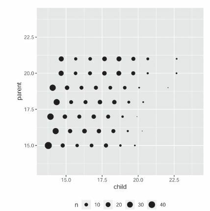
Table 1 Contingency table for Galton’s peas data.

	Parent
Child	15	16	17	18	19	20	21
13.77	46	0	0	0	0	0	0
13.92	0	0	37	0	0	0	0
14.07	0	0	0	0	35	0	0
14.28	0	34	0	0	0	0	0
14.35	0	0	0	34	0	0	0
14.66	0	0	0	0	0	23	0
14.67	0	0	0	0	0	0	22
14.77	14	0	0	0	0	0	0
14.92	0	0	16	0	0	0	0
15.07	0	0	0	0	16	0	0
15.28	0	15	0	0	0	0	0
15.35	0	0	0	12	0	0	0
15.66	0	0	0	0	0	10	0
15.67	0	0	0	0	0	0	8
15.77	9	0	0	0	0	0	0
15.92	0	0	13	0	0	0	0
16.07	0	0	0	0	12	0	0
16.28	0	18	0	0	0	0	0
16.35	0	0	0	13	0	0	0
16.66	0	0	0	0	0	12	0
16.67	0	0	0	0	0	0	10
16.77	11	0	0	0	0	0	0
16.92	0	0	16	0	0	0	0
17.07	0	0	0	0	13	0	0
17.28	0	16	0	0	0	0	0
17.35	0	0	0	17	0	0	0
	Parent
Child	15	16	17	18	19	20	21
17.66	0	0	0	0	0	17	0
17.67	0	0	0	0	0	0	18
17.77	14	0	0	0	0	0	0
17.92	0	0	13	0	0	0	0
18.07	0	0	0	0	11	0	0
18.28	0	13	0	0	0	0	0
18.35	0	0	0	16	0	0	0
18.66	0	0	0	0	0	20	0
18.67	0	0	0	0	0	0	21
18.77	4	0	0	0	0	0	0
18.92	0	0	4	0	0	0	0
19.07	0	0	0	0	10	0	0
19.28	0	3	0	0	0	0	0
19.35	0	0	0	6	0	0	0
19.66	0	0	0	0	0	13	0
19.67	0	0	0	0	0	0	13
19.77	2	0	0	0	0	0	0
19.92	0	0	1	0	0	0	0
20.07	0	0	0	0	2	0	0
20.28	0	1	0	0	0	0	0
20.35	0	0	0	2	0	0	0
20.66	0	0	0	0	0	3	0
20.67	0	0	0	0	0	0	6
22.07	0	0	0	0	1	0	0
22.66	0	0	0	0	0	2	0
22.67	0	0	0	0	0	0	2

For example, among all mother plants with mean diameter 15, there were 46 cases where the daughter plant had diameter 13.77, 14 had diameter 14.77, 11 had diameter 16.77, 14 had diameter 17.77, and 4 had diameter 18.77. On the other hand, for all 46 daughter plants in the data with diameter 13.77, the mother plants had diameter 15. Similarly, for all 34 daughter plants with diameter 14.28, the mother plants had diameter 16.

Common sense suggests that the reason behind this strange phenomenon is surely some quirk of the data collection or recording method, and not some profound biological fact. (It is probably not a simple rounding effect, though; for instance, in all 46 cases where Y = 13.77, we have X = 15, but for all 37 cases where Y = 13.92, which is only slightly different than 13.77, we have X = 17.) However, if we imagine that the values recorded in the data are the exact values that were measured and the observations were iid (neither of which is exactly true, as I learned from Steve Stigler), then looking at Table 1 there is no way to escape the conclusion that the mean diameter of peas in the mother plant can be exactly predicted with considerable certainty by the mean diameter of the peas in the daughter plant (but not the other way around). The coefficient ${\xi }_n(Y,X)$ discovers this fact numerically by attaining a value close to 1. It is probable that this feature of Galton’s peas data has been noted before, but if so, it is certainly hard to find. I could not find any reference where this is mentioned, in spite of much effort.

4 Simulation Results

The goal of this section is to investigate the performance of ξ_n using numerical simulations, and compare it to other methods. We compare general performance, run times, and powers for testing independence.

4.1 General Performance, Equitability, and Generality

Figure 2 gives a glimpse of the general performance of ξ_n as a measure of association. The figure has three rows. Each row starts with a scatterplot where Y is a noiseless function of X, and X is generated from the uniform distribution on $[-1,1]$. As we move to the right, more and more noise is added. The sample size n is taken to be 100 in each case, to show that ξ_n performs well in relatively small samples. In each row, we see that ${\xi }_n(X,Y)$ is very close 1 for the leftmost graph, and progressively deteriorates as we add more noise. By Theorem 2.1, the 95th percentile of ${\xi }_n(X,Y)$ under the hypothesis of independence, for n = 100, is approximately 0.066. The values in Figure 2 are all much higher than that.

Fig. 2 Values of ${\xi }_n(X,Y)$ for various kinds of scatterplots, with n = 100. Noise increases from left to right. The 95th percentile of ${\xi }_n(X,Y)$ under the hypothesis of independence is approximately 0.066.

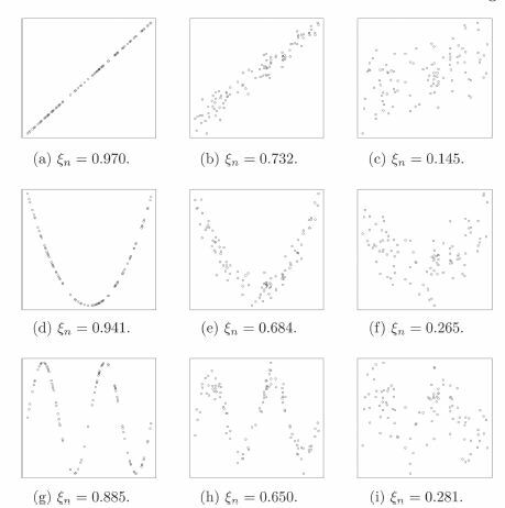
An interesting observation from Figure 2 is that ξ_n appears to be an equitable coefficient, as defined in Reshef et al. (2011). The definition of equitability is not mathematically precise but intuitively clear. Roughly, an equitable measure of correlation “gives similar scores to equally noisy relationships of different types.” Figure 2 indicates that ξ_n has this property as long as the relationship is “functional.” It is not equitable for relationships that are not functional, although that is expected because ξ_n measures how well Y can be predicted by X.

The other criterion for a good measure of correlation, according to Reshef et al. (2011), is that the coefficient should be “general,” in that it should be able to detect any kind of pattern in the scatterplot. In statistical terms, this means that the test of independence based on the coefficient should be consistent against all alternatives. This is clearly true by Theorem 1.1, in fact more true than for any other coefficient in the literature. Among available test statistics, only maximal correlation has this property in full generality, but there is no estimator of maximal correlation that is known to be consistent for all possible distributions of (X, Y).

4.2 Validity of the Asymptotic Theory

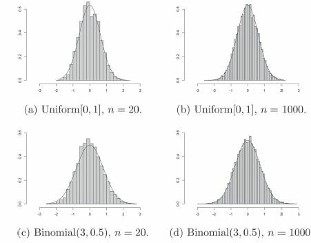
Next, let us numerically investigate the distribution of ${\xi }_n(X,Y)$ when X and Y are independent. Taking X_i’s and Y_i’s to be independent Uniform$[0,1]$ random variables, and n = 20, 10,000 values of ${\xi }_n(X,Y)$ were generated. The histogram of $\sqrt{n}{\xi }_n(X,Y)$ is displayed in Figure 3(a), superimposed with the asymptotic density function predicted by Theorem 2.1. We see that already for n = 20, the agreement is striking. A much better agreement is obtained with n = 1000 in Figure 3(b). Next, X_i’s and Y_i’s were drawn as independent Binomial$(3,0.5)$ random variables. The value of ${\tau }^2$ was estimated using Theorem 2.3, and was plugged into Theorem 2.2 to obtain the asymptotic distribution of $\sqrt{n}{\xi }_n$. Again, the true distributions are shown to be in good agreement with the asymptotic distributions, for n = 20 and n = 1000, in Figures 3(c) and (d).

Fig. 3 Histogram of 10,000 simulations of $\sqrt{n}{\xi }_n$, superimposed with the asymptotic density function.

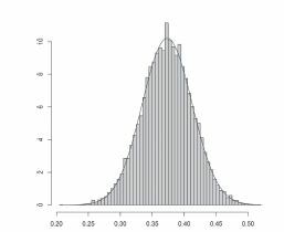
Some simulation analysis was also carried out to investigate the convergence of ξ_n under dependence. For that, the following simple model was chosen. Let $X\sim \text{Bernoulli}(p)$ and $Z\sim \text{Bernoulli}(p\prime )$ be independent random variables, and let $Y:=XZ$. Then X and Y are dependent Bernoulli random variables. An easy calculation shows that$$\xi (X,Y)=\frac{p\prime (1-p)}{1-pp\prime }.$$

With p = 0.4 and $p\prime =0.5$, we get $\xi (X,Y)=0.375$. To test the convergence of ξ_n to ξ, 10,000 simulations were carried out with n = 1000. In this sample, the mean value of ξ_n was approximately 0.374 and the standard deviation was approximately 0.040 (which means that the standard deviation of $\sqrt{n}{\xi }_n$ was approximately 1.254). The histogram given in Figure 4 shows an excellent fit with a normal distribution with the above mean and standard deviation.

Fig. 4 Histogram of 10,000 simulations of ${\xi }_n(X,Y)$ when X and Y are dependent Bernoulli random variables (see Section 4.2), superimposed with the normal density function of suitable mean and variance. Here, $\xi (X,Y)=0.375$ and n = 1000.

4.3 Power and Run Time Comparisons

In this section, we compare the power of the test of independence based on ξ_n against a number of powerful tests proposed in recent years, and we also compare the run times of these tests. The main finding is that ξ_n is less powerful than some of the other tests if the signal is relatively smooth, and more powerful if the signal is wiggly. In terms of run time, ξ_n has a big advantage since it is computable in time $O(n\hspace{0.17em}\text{log}\hspace{0.17em}n)$, whereas its competitors require time n². This is further validated through numerical examples, which show that ξ_n is essentially the only statistic that can be computed in reasonable time if the sample size is in the order several thousands.

Comparisons are carried out with the following popular test statistics for testing independence. I excluded statistics that are either too new (because they are not time-tested, and software is not available in many cases) or too old (because they are superseded by newer ones). In the following, $(X_1,Y_1),\dots ,(X_n,Y_n)$ is an iid sample of points from some distribution on ${\mathbb{R}}^2$.

1. Maximal information coefficient (MIC) (Reshef et al. 2011): Recall that the mutual information of a bivariate probability distribution is the Kullback–Leibler divergence between that distribution and the product of its marginals. Given any scatterplot of n points, suppose we divide it into an x × y array of rectangles. The proportions of points falling into these rectangles define a bivariate probability distribution. Let I be the mutual information of this probability distribution. The maximum of $I/\hspace{0.17em}\text{log}\hspace{0.17em}\min \{x,y\}$ over all subdivisions into rectangles, under the constraint $xy<n^{0.6}$, is called the maximal information coefficient of the scatterplot.

2. Distance correlation (Székely, Rizzo, and Bakirov 2007): Let $a_{ij}:=|X_i-X_j|$ and $b_{ij}:=|Y_i-Y_j|$. Center these numbers by defining $A_{ij}:=a_{ij}-a_{i·}-a_{·j}+a_{··}$ and $B_{ij}:=b_{ij}-b_{i·}-b_{·j}+b_{··}$, where $a_{i·}$ is the average of a_ij over all j, etc. The distance correlation between the two samples is simply the Pearson correlation between the A_ij’s and the B_ij’s.

3. The HHG test (Heller, Heller, and Gorfine 2013): Take any i and j. Divide X_k’s into two groups depending on whether $|X_i-X_k|<|X_i-X_j|$ or not. Similarly classify the Y_k’s into two groups depending on whether $|Y_i-Y_k|<|Y_i-Y_j|$ or not. These classifications partition the scatterplot into four compartments, and the numbers of points in these compartments define a 2 × 2 contingency table. The HHG test statistic is a linear combination of the Pearson ${\chi }^2$ statistics for testing independence in these contingency tables over all choices of i and j.

4. The Hilbert–Schmidt independence criterion (HSIC) (Gretton et al. 2005, 2008): Let k and l be symmetric positive definite kernels on ${\mathbb{R}}^2$. For example, we may take the Gaussian kernel $k(x,y)=l(x,y)=e^{-|x-y{|}^2/2{\sigma }^2}$ for some $\sigma >0$. Let $k_{ij}:=k(X_i,X_j)$ and $l_{ij}:=l(Y_i,Y_j)$. Then the HSIC statistic is$$\frac{1}{n^2}\sum _{i,j}{k}_{ij}{l}_{ij}+\frac{1}{n^4}\sum _{i,j,q,r}{k}_{ij}{l}_{qr}-\frac{2}{n^3}\sum _{i,j,q}{k}_{ij}{l}_{iq}.$$

All of the above test statistics are consistent for testing independence under mild conditions. Moreover, the HSIC test has been proved to be minimax rate-optimal against uniformly smooth alternatives (Li and Yuan 2019).

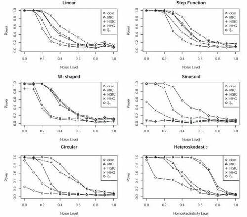
Power comparisons were carried out with sample size n = 100. In each case, 500 simulations were used to estimate the power. The R packages energy, minerva, HHG, and dHSIC were used for calculating the distance correlation, MIC, HHG, and HSIC statistics, respectively. Since the HHG test is very slow for large samples, a fast univariate version of the HHG test (Heller et al. 2016) was used. Generating X from the uniform distribution on $[-1,1]$, the following six alternatives were considered:

1. Linear: $Y=0.5X+3\lambda \epsilon$, where λ is a noise parameter ranging from 0 to 1, and $\epsilon \sim N(0,1)$ is independent of X.

2. Step function: $Y=f(X)+10\lambda \epsilon$, where f takes values –3, 2, –4, and –3 in the intervals $[-1,-0.5),[-0.5,0),[0,0.5)$, and $[0.5,1]$.

3. W-shaped: $Y=|X+0.5|1_{\{X<0\}}+|X-0.5|1_{\{X\ge 0\}}+0.75\lambda \epsilon$.

4. Sinusoid: $Y=\hspace{0.17em}\text{cos}\hspace{0.17em}8\pi X+3\lambda \epsilon$.

5. Circular: $Y=Z\sqrt{1-X^2}+0.9\lambda \epsilon$, where Z is 1 or –1 with equal probability, independent of X.

6. Heteroscedastic: $Y=3(\sigma (X)(1-\lambda )+\lambda )\epsilon$, where $\sigma (X)=1$ if $\left|X\right|\le 0.5$ and 0 otherwise. As λ increases from 0 to 1, the relationship becomes more and more homoscedastic.

The coefficients in all of the above were chosen to ensure that a full range of powers were observed as λ was varied from 0 to 1. The results are presented in Figure 5. The main observation from this figure is that ξ_n is more powerful than the other tests when the signal has an oscillatory nature, such as for the W-shaped scatterplot and the sinusoid. For the step function, too, it performs reasonably well. However, ξ_n has inferior performance for smoother alternatives, namely, the linear, circular, and heteroscedastic scatterplots.

Fig. 5 Comparison of powers of several tests of independence. The titles describe the shapes of the scatterplots. The level of the noise increases from left to right. In each case, the sample size is 100, and 500 simulations were used to estimate the power.

Next, let us turn to the comparison of run times for tests of independence based on the five competing test statistics. For all except ξ_n, the only way to test for independence is to run a permutation test. (There is a theoretical test for HSIC, but it is only a crude approximation.) The number of permutations was taken to be the smallest respectable number, 200. Usually 200 is too small for a permutation test, but I took it to be so small so that the program terminates in a manageable amount of time for the larger values of n. For ξ_n, the asymptotic test was used because it performs as well as the permutation test even in very small samples, as we saw in Section 4.2.

For distance correlation, HSIC, and HHG, the permutation tests are directly available from the corresponding R packages. For MIC, I had to write the code because the permutation tests are not automatically available from the package, so the run time can probably be somewhat improved with a better code. For the HHG test, the function requires the distance matrices for X and Y to be input as arguments. For the sake of fairness, the time required for computing the distance matrices was included in the total time for carrying out the permutation tests.

The results are presented in Table 2. Every test was hundreds or even thousands of times slower than the test based on ξ_n for all sample sizes 500 and above. For sample size 10,000, the HHG test was terminated after not converging in 30 min.

Table 2 Run times (in sec) for permutation tests of independence, with 200 permutations.

n	dCor	MIC	HSIC	HHG	ξn
100	0.008	0.328	0.048	0.167	0.006
500	0.104	5.433	1.214	4.671	0.007
1000	0.532	17.459	5.028	20.515	0.009
2000	2.423	55.556	18.873	108.949	0.009
10,000	88.976	1097.483	860.605	>30 min	0.011

NOTE: For ξ_n, the asymptotic test was used because it is as reliable as the permutation test.

5 Example: Yeast Gene Expression Data

In a landmark paper in gene expression studies (Spellman et al. 1998), the authors studied the expressions of 6223 yeast genes with the goal of identifying genes whose transcript levels oscillate during the cell cycle. In lay terms, this means that the expressions were studied over a number of successive time points (23, to be precise), and the goal was to identify the genes for which the transcript levels follow an oscillatory pattern. This example illustrates the utility of correlation coefficients in detecting patterns, because the number of genes is so large that identifying patterns by visual inspection is out of the question.

This dataset was used in the paper (Reshef et al. 2011) to demonstrate the efficacy of MIC for identifying patterns in scatterplots. The authors of Reshef et al. (2011) used a curated version of the dataset, where they excluded all genes for which there were missing observations, and made several other modifications. The revised dataset has 4381 genes. I used this curated dataset (available through the R package minerva) to study the power of ξ_n in discovering genes with oscillating transcript levels, and compare its performance with the competing tests from Section 4.3.

There are literally hundreds of papers analyzing this particular dataset. I will not attempt to go deep into this territory in any way, because that will take us too far afield. The sole purpose of the analysis that follows is to compare the performance of ξ_n with the competing tests.

For each test, p-values were obtained and a set of significant genes were selected using the Benjamini–Hochberg FDR procedure (Benjamini and Hochberg 1995), with the expected proportion of false discoveries set at 0.05.

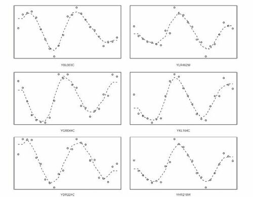
It turned out that there are 215 genes (out of 4381) that are selected by ξ_n but by none of the other tests. This is surprising in itself, but what is more surprising is the nature of these genes. Figure 6 shows the transcript levels of the top 6 of these genes (that is, those with the smallest p-values). There is no question that these genes exhibit almost perfect oscillatory behavior and yet they were not selected by any of the other tests.

Fig. 6 Transcript levels of the top 6 among the 215 genes selected by ξ_n but by no other test. The dashed lines are fitted by k-nearest neighbor regression with k = 3. The name of the gene is displayed below each plot.

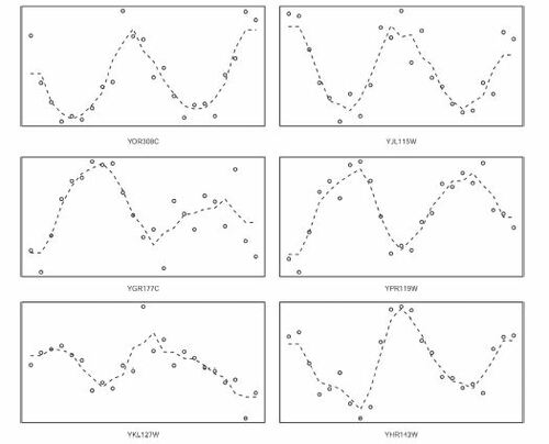
One may wonder if this is true for only the top 6 genes, or typical of all 215. To investigate that, I took a random sample of 6 genes from the 215, and looked at their transcript levels. The results are shown in Figure 7. Even for a random sample, we see strong oscillatory behavior. This behavior was consistently observed in other random samples.

Fig. 7 Transcript levels of a random sample of 6 genes from the 215 genes that were selected by ξ_n but by no other test.

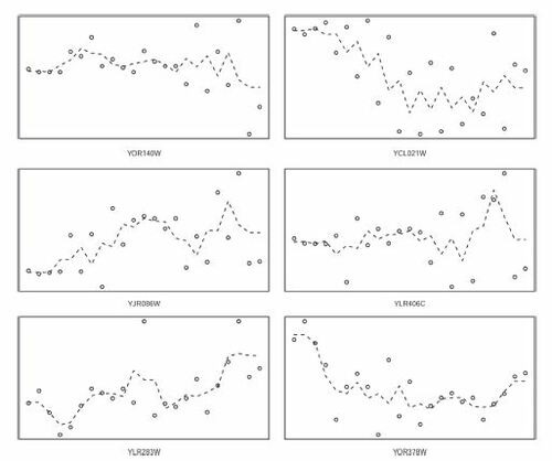
How about the genes that were selected by at least one of the other tests, but not by ξ_n? Figure 8 shows the transcript levels of a random sample of 6 genes selected from this set. I think it is reasonable to say that these plots show slight increasing or decreasing trends, or heteroscedasticity, but no definite oscillatory patterns. Repeated samplings showed similar results.

Fig. 8 Transcript levels of 6 randomly sampled genes from the set of genes that were not selected by ξ_n but were selected by at least one other test.

Thus, we arrive at the following conclusion. The genes selected by ξ_n are much more likely than the genes selected by the other tests to be the ones that really exhibit oscillatory patterns in their transcript levels during the cell cycle. This is because the other tests prioritize monotone trends over cyclical patterns. Most of the 215 genes that were selected by ξ_n but not by any of the other tests show pronounced oscillatory patterns. The fact that ξ_n is particularly powerful for detecting oscillatory behavior turns out to be very useful in this example. Of course, ξ_n also selects genes that show other kinds of patterns (it selects a total of 586 genes), but those are selected by at least one of the other tests and therefore do not appear in this set of 215 genes that are selected exclusively by ξ_n.

6 MIC and Maximal Correlation May Not Correctly Measure the Strength of the Relationship

It is sometimes mistakenly believed that MIC and maximal correlation measure the strength of relationship between X and Y; in particular, that they attain their maximum value, 1, if and only if the relationship between X and Y is perfectly noiseless. In this section we show that this is not true: MIC and maximal correlation can detect noiseless relationships even if the actual relationship between X and Y is very noisy.

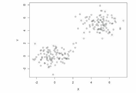
In the example shown in Figure 9, 200 samples of (X, Y) are generated from a mixture of bivariate normal distributions. With probability 1/2, (X, Y) is drawn from the standard bivariate normal distribution, and with probability 1/2, (X, Y) is drawn from the bivariate normal distribution with mean (5, 5) and identity covariance matrix. The data forms two clusters of roughly equal size that are close but nearly disjoint. Clearly, there is a lot of noise in the relationship between X and Y. Given X, we can only tell whether Y comes from N(0, 1) or N(5, 1), but nothing else. Yet, rounded off to two decimal places, MIC is 1.00 and maximal correlation (as computed by the ACE algorithm, Breiman and Friedman 1985) is 0.99 for this scatterplot. The coefficient ξ_n, on the other hand, is well-behaved; it turns out to be 0.48, indicating the presence of a significant relationship between X and Y but not a noiseless one. Common sense suggests that the value 0.48 is much better reflective of the strength of the relationship between X and Y in Figure 9 than 0.99 or 1.00.

Fig. 9 Scatterplot of a mixture of bivariate normals, with n = 200. For this plot, maximal correlation $=0.99$, MIC $=1.00$, and ${\xi }_n=0.48$.

In the supplementary materials of Reshef et al. (2011), it is shown that MIC =1 when $Y=f(X)$ for a large class of functions f. However, it is not shown that the converse is true, that is MIC =1 implies that X and Y have a noiseless relationship. Figure 9 indicates that in fact the converse is probably not true. The phenomenon is not an artifact of the sample size—it remains consistently true in larger sample sizes. Moreover, scatterplots such as Figure 9 are not uncommon in real datasets.

The following mathematical result uses the intuition gained from the above example to confirm that there indeed exist very noisy relationships which are declared to be perfectly noiseless by maximal correlation and MIC.

Proposition 6.1.

Let I₁, I₂, J₁, and J₂ be bounded intervals such that I₁ and I₂ are disjoint, and J₁ and J₂ are disjoint. Suppose that the law of a random vector (X, Y) is supported on the union of the two rectangles $I_1\times J_1$ and $I_2\times J_2$, giving equal masses to both. Then the maximal correlation between X and Y is 1, and the MIC between X and Y in an iid sample of size n tends to 1 in probability as $n\to \infty$.

Proof.

Recall that the maximal correlation between two random variables X and Y is defined as the maximum possible correlation between f(X) and g(Y) over all f and g such that f(X) and g(Y) are square-integrable. In the setting of this proposition, let f be the indicator of the interval I₁ and g be the indicator of the interval J₁. Then f(X) = 1 if and only if g(Y) = 1, because the nature of (X, Y) implies that $X\in I_1$ if and only if $Y\in J_1$. Thus, $f(X)=g(Y)$, and so the maximal correlation between X and Y is equal to 1.

Next, recall the definition of MIC from Section 4.3. The support of (X, Y) can be partitioned into the 2 × 2 array of rectangles $I_1\times J_1,I_1\times J_2,I_2\times J_1$, and $I_2\times J_2$. The first and fourth rectangles carry mass 1/2 each, and the other two carry mass 0. Therefore, when n is large, the first and fourth rectangles receive approximately $n/2$ points each, and the other two receive no points. A simple calculation shows that the mutual information of the corresponding contingency table is approximately $\text{log}\hspace{0.17em}2$. Thus, the contribution of this array of rectangles to the definition of MIC is approximately 1, which shows that the MIC itself is approximately 1 (since it cannot exceed 1 and is defined to be the maximum of the contributions from all rectangular partitions of size $<n^{0.6}$). □

7 Summary

Let us now briefly summarize what we learned. The new correlation coefficient offers many advantages over its competitors. The following is a partial list:

1. It has a very simple formula. The formula is as simple as those for the classical coefficients, like Pearson’s correlation, Spearman’s ρ, or Kendall’s τ.

2. Due to its simple formula, it is (a) easy to understand conceptually, and (b) computable very quickly, not only in theory but also in practice. Most of its competitors are hundreds of times slower to compute even in samples of moderately large size, such as 500.

3. It is a function of ranks, which makes it robust to outliers and invariant under monotone transformations of the data.

4. It converges to a limit which has an easy interpretation as a measure of dependence. The limit ranges from 0 to 1. It is 1 if and only if Y is a measurable function of X and 0 if and only if X and Y are independent. Thus, ξ_n gives an actual measure of the strength of the relationship.

5. It has a very simple asymptotic theory under the hypothesis of independence, which is roughly valid even for samples of size as small as 20. This allows theoretical tests of independence, bypassing computationally expensive permutation tests that are necessary for other tests.

6. The test of independence based on ξ_n is consistent against all alternatives, with no exceptions. No other test has this property.

7. None of the results mentioned above require any assumptions about the law of (X, Y) except that Y is not a constant. One can even apply ξ_n to categorical data, by converting the categorical variables to integer-valued variables in any arbitrary way.

8. In simulations and real data, ξ_n seems to be more powerful than other tests for detecting oscillatory signals.

Against all of the above advantages, ξ_n has only one disadvantage: It seems to have less power than several popular tests of independence when the signal is smooth and nonoscillatory. Although such signals comprise the majority of types observed in practice, this is a matter of concern only when the sample size is small. In large samples, all tests are powerful, and computational time becomes a much bigger concern.

8 Proof Sketch

This section contains a brief sketch of the proof of convergence of ξ_n to ξ. For simplicity, let us only consider the case of continuous X and Y. First, note that by the Glivenko–Cantelli theorem, $r_i/n\approx F(Y_{(i)})$, where F is the cumulative distribution function of Y. Thus,(5) $${\xi }_n(X,Y)\approx 1-\frac{3}{n}\sum _{i=1}^n|F(Y_i)-F(Y_{N(i)})|,$$(5) where N(i) is the unique index j such that X_j is immediately to the right of X_i if we arrange the X’s in increasing order. If X_i is the rightmost value, define N(i) arbitrarily; it does not matter since the contribution of a single term in the above sum is $O(1/n)$.

The first important observation is that for any $x,y\in \mathbb{R}$,(6) $$|F(x)-F(y)|=\int {(1_{\{t\le x\}}-1_{\{t\le y\}})}^{2}d\mu (t),$$(6) where μ is the law of Y. This is true because the integrand is 1 between x and y and 0 outside.

Now suppose that we condition on $X_1,\dots ,X_n$. Since X_i is likely to be very close to $X_{N(i)}$, the random variables Y_i and $Y_{N(i)}$ are likely to be approximately iid after this conditioning. This is the second key observation (which is tricky to make rigorous in the absence of any assumptions on the law of (X, Y)), which leads to the approximation$$\begin{array}{c}\mathbb{E}\left[{(1_{\{t\le Y_i\}}-1_{\{t\le Y_{N(i)}\}})}^2\right|X_1,\dots ,X_n]\approx 2\text{var}(1_{\{t\le Y_i\}}|X_1,\dots ,X_n)\\ =2\text{var}(1_{\{t\le Y_i\}}|X_i).\end{array}$$

This gives$$\begin{array}{c}\mathbb{E}{(1_{\{t\le Y_i\}}-1_{\{t\le Y_{N(i)}\}})}^2\approx 2\mathbb{E}[\text{var}(1_{\{t\le Y\}}|X)]\\ =2\text{var}(1_{\{t\le Y\}})-2\text{var}(\mathbb{E}(1_{\{t\le Y\}}|X)).\end{array}$$

Combining this with (6), we get$$\begin{array}{c}\mathbb{E}|F(Y_i)-F(Y_{N(i)})|\\ \hspace{1em}\approx \int 2[\text{var}(1_{\{t\le Y\}})-\text{var}(\mathbb{E}(1_{\{t\le Y\}}|X))]d\mu (t).\end{array}$$

But note that $\text{var}(1_{\{t\le Y\}})=F(t)(1-F(t))$, and $F(Y)\sim \text{Uniform}[0,1]$. Thus,$$\begin{array}{c}\int \text{var}(1_{\{t\le Y\}})d\mu (t)=\int F(t)(1-F(t))d\mu (t)\\ ={\int }_0^{1}x(1-x)dx=\frac{1}{6}.\end{array}$$

Therefore by (5),$$\mathbb{E}({\xi }_n(X,Y))\approx 6\int \text{var}(\mathbb{E}(1_{\{t\le Y\}}|X))d\mu (t)=\xi (X,Y),$$where the last identity holds because $\int \text{var}(1_{\{t\le Y\}})d\mu (t)=1/6$, as shown above. This establishes the convergence of $\mathbb{E}({\xi }_n(X,Y))$ to $\xi (X,Y)$. Concentration inequalities are then used to show that ${\xi }_n(X,Y)-\mathbb{E}({\xi }_n(X,Y))\to 0$ almost surely.

Supplementary Materials

The supplementary material consists of a single pdf file containing the proofs of Theorems 1.1, 2.2 and 2.3. (Theorem 2.1 is a special case of Theorem 2.2, so it does not have a separate proof.)

Acknowledgments

I thank Mona Azadkia, Peter Bickel, Holger Dette, Mathias Drton, Lihua Lei, Bodhisattva Sen, Rik Sen, and Steve Stigler for a number of useful comments and references. I am especially grateful to Persi Diaconis and Susan Holmes for many suggestions that greatly improved the article. Lastly, I thank the anonymous referees for a number of suggestions that helped improve the presentation.

Additional information

Funding

Research partially supported by NSF grant DMS-1855484.

References

- Azadkia, M., and Chatterjee, S. (2019), “A Simple Measure of Conditional Dependence,” arXiv no. 1910.12327.
- Benjamini, Y., and Hochberg, Y. (1995), “Controlling the False Discovery Rate: A Practical and Powerful Approach to Multiple Testing,” Journal of the Royal Statistical Society, Series B, 57, 289–300. DOI: https://doi.org/10.1111/j.2517-6161.1995.tb02031.x.
- Bergsma, W., and Dassios, A. (2014), “A Consistent Test of Independence Based on a Sign Covariance Related to Kendall’s Tau,” Bernoulli, 20, 1006–1028. DOI: https://doi.org/10.3150/13-BEJ514.
- Blum, J. R., Kiefer, J., and Rosenblatt, M. (1961), “Distribution Free Tests of Independence Based on the Sample Distribution Function,” The Annals of Mathematical Statistics, 32, 485–498. DOI: https://doi.org/10.1214/aoms/1177705055.
- Breiman, L., and Friedman, J. H. (1985), “Estimating Optimal Transformations for Multiple Regression and Correlation,” Journal of the American Statistical Association, 80, 580–598. DOI: https://doi.org/10.1080/01621459.1985.10478157.
- Chao, C.-C., Bai, Z., and Liang, W.-Q. (1993), “Asymptotic Normality for Oscillation of Permutation,” Probability in the Engineering and Informational Sciences, 7, 227–235. DOI: https://doi.org/10.1017/S0269964800002886.
- Chatterjee, S., and Holmes, S. (2020), “XICOR: Association Measurement Through Cross Rank Increments,” R Package, available at https://CRAN.R-project.org/package=XICOR.
- Csörgő, S. (1985), “Testing for Independence by the Empirical Characteristic Function,” Journal of Multivariate Analysis, 16, 290–299. DOI: https://doi.org/10.1016/0047-259X(85)90022-3.
- Deb, N., and Sen, B. (2019), “Multivariate Rank-Based Distribution-Free Nonparametric Testing Using Measure Transportation,” arXiv no. 1909.08733.
- Dette, H., Siburg, K. F., and Stoimenov, P. A. (2013), “A Copula-Based Non-Parametric Measure of Regression Dependence,” Scandinavian Journal of Statistics, 40, 21–41. DOI: https://doi.org/10.1111/j.1467-9469.2011.00767.x.
- Drton, M., Han, F., and Shi, H. (2018), “High Dimensional Independence Testing With Maxima of Rank Correlations,” arXiv no. 1812.06189.
- Friedman, J. H., and Rafsky, L. C. (1983), “Graph-Theoretic Measures of Multivariate Association and Prediction,” The Annals of Statistics, 11, 377–391. DOI: https://doi.org/10.1214/aos/1176346148.
- Gamboa, F., Klein, T., and Lagnoux, A. (2018), “Sensitivity Analysis Based on Cramér–von Mises Distance,” SIAM/ASA Journal on Uncertainty Quantification, 6, 522–548. DOI: https://doi.org/10.1137/15M1025621.
- Gebelein, H. (1941), “Das statistische Problem der Korrelation als Variations- und Eigenwertproblem und sein Zusammenhang mit der Ausgleichsrechnung,” Zeitschrift für Angewandte Mathematik und Physik, 21, 364–379. DOI: https://doi.org/10.1002/zamm.19410210604.
- Gretton, A., Bousquet, O., Smola, A., and Schölkopf, B. (2005), “Measuring Statistical Dependence With Hilbert–Schmidt Norms,” in Algorithmic Learning Theory, Berlin: Springer, pp. 63–77.
- Gretton, A., Fukumizu, K., Teo, C. H., Song, L., Schölkopf, B., and Smola, A. J. (2008), “A Kernel Statistical Test of Independence,” in Advances in Neural Information Processing Systems, pp. 585–592.
- Han, F., Chen, S., and Liu, H. (2017), “Distribution-Free Tests of Independence in High Dimensions,” Biometrika, 104, 813–828. DOI: https://doi.org/10.1093/biomet/asx050.
- Heller, R., Heller, Y., and Gorfine, M. (2013), “A Consistent Multivariate Test of Association Based on Ranks of Distances,” Biometrika, 100, 503–510. DOI: https://doi.org/10.1093/biomet/ass070.
- Heller, R., Heller, Y., Kaufman, S., Brill, B., and Gorfine, M. (2016), “Consistent Distribution-Free K-Sample and Independence Tests for Univariate Random Variables,” Journal of Machine Learning Research, 17, 978–1031.
- Hirschfeld, H. O. (1935), “A Connection Between Correlation and Contingency,” Mathematical Proceedings of the Cambridge Philosophical Society, 31, 520–524. DOI: https://doi.org/10.1017/S0305004100013517.
- Hoeffding, W. (1948), “A Non-Parametric Test of Independence,” The Annals of Mathematical Statistics, 19, 546–557. DOI: https://doi.org/10.1214/aoms/1177730150.
- Josse, J., and Holmes, S. (2016), “Measuring Multivariate Association and Beyond,” Statistics Surveys, 10, 132–167. DOI: https://doi.org/10.1214/16-SS116.
- Kraskov, A., Stogbauer, H., and Grassberger, P. (2004), “Estimating Mutual Information,” Physical Review E, 69, 066138. DOI: https://doi.org/10.1103/PhysRevE.69.066138.
- Li, T., and Yuan, M. (2019), “On the Optimality of Gaussian Kernel Based Nonparametric Tests against Smooth Alternatives,” arXiv no. 1909.03302.
- Linfoot, E. H. (1957), “An Informational Measure of Correlation,” Information and Control, 1, 85–89. DOI: https://doi.org/10.1016/S0019-9958(57)90116-X.
- Lopez-Paz, D., Hennig, P., and Schölkopf, B. (2013), “The Randomized Dependence Coefficient,” in Advances in Neural Information Processing Systems, pp. 1–9.
- Lyons, R. (2013), “Distance Covariance in Metric Spaces,” Annals of Probability, 41, 3284–3305. DOI: https://doi.org/10.1214/12-AOP803.
- Nandy, P., Weihs, L., and Drton, M. (2016), “Large-Sample Theory for the Bergsma–Dassios Sign Covariance,” Electronic Journal of Statistics, 10, 2287–2311. DOI: https://doi.org/10.1214/16-EJS1166.
- Pfister, N., Bühlmann, P., Schölkopf, B., and Peters, J. (2018), “Kernel-Based Tests for Joint Independence,” Journal of the Royal Statistical Society, Series B, 80, 5–31. DOI: https://doi.org/10.1111/rssb.12235.
- Puri, M. L., and Sen, P. K. (1971), Nonparametric Methods in Multivariate Analysis, New York: Wiley.
- Rényi, A. (1959), “On Measures of Dependence,” Acta Mathematica Hungarica, 10, 441–451. DOI: https://doi.org/10.1007/BF02024507.
- Reshef, D. N., Reshef, Y. A., Finucane, H. K., Grossman, S. R., McVean, G., Turnbaugh, P. J., Lander, E. S., Mitzenmacher, M., and Sabeti, P. (2011), “Detecting Novel Associations in Large Datasets,” Science, 334, 1518–1524. DOI: https://doi.org/10.1126/science.1205438.
- Romano, J. P. (1988), “A Bootstrap Revival of Some Nonparametric Distance Tests,” Journal of the American Statistical Association, 83, 698–708. DOI: https://doi.org/10.1080/01621459.1988.10478650.
- Rosenblatt, M. (1975), “A Quadratic Measure of Deviation of Two-Dimensional Density Estimates and a Test of Independence,” The Annals of Statistics, 3, 1–14. DOI: https://doi.org/10.1214/aos/1176342996.
- Sarkar, S., and Ghosh, A. K. (2018), “Some Multivariate Tests of Independence Based on Ranks of Nearest Neighbors,” Technometrics, 60, 101–111. DOI: https://doi.org/10.1080/00401706.2016.1278182.
- Schweizer, B., and Wolff, E. F. (1981), “On Nonparametric Measures of Dependence for Random Variables,” The Annals of Statistics, 9, 879–885. DOI: https://doi.org/10.1214/aos/1176345528.
- Sen, A., and Sen, B. (2014), “Testing Independence and Goodness-of-Fit in Linear Models,” Biometrika, 101, 927–942. DOI: https://doi.org/10.1093/biomet/asu026.
- Sklar, M. (1959), “Fonctions de répartition à n dimensions et leurs marges,” Publ. Inst. Stat. Univ. Paris, 8, 229–231.
- Spellman, P. T., Sherlock, G., Zhang, M. Q., Iyer, V. R., Anders, K., Eisen, M. B., Brown, P. O., Botstein, D., and Futcher, B. (1998), “Comprehensive Identification of Cell Cycle-Regulated Genes of the Yeast Saccharomyces cerevisiae by Microarray Hybridization,” Molecular Biology of the Cell, 9, 3273–3297. DOI: https://doi.org/10.1091/mbc.9.12.3273.
- Stigler, S. M. (1986), The History of Statistics: The Measurement of Uncertainty Before 1900, Cambridge, MA: Harvard University Press. DOI: https://doi.org/10.1086/ahr/93.4.1019.
- Székely, G. J., and Rizzo, M. L. (2009), “Brownian Distance Covariance,” The Annals of Applied Statistics, 3, 1236–1265. DOI: https://doi.org/10.1214/09-AOAS312.
- Székely, G. J., Rizzo, M. L., and Bakirov, N. K. (2007), “Measuring and Testing Dependence by Correlation of Distances,” The Annals of Statistics, 35, 2769–2794. DOI: https://doi.org/10.1214/009053607000000505.
- Wang, X., Jiang, B., and Liu, J. S. (2017), “Generalized R-Squared for Detecting Dependence,” Biometrika, 104, 129–139. DOI: https://doi.org/10.1093/biomet/asw071.
- Weihs, L., Drton, M., and Leung, D. (2016), “Efficient Computation of the Bergsma-Dassios Sign Covariance,” Computational Statistics, 31, 315–328. DOI: https://doi.org/10.1007/s00180-015-0639-x.
- Weihs, L., Drton, M., and Meinshausen, N. (2018), “Symmetric Rank Covariances: A Generalized Framework for Nonparametric Measures of Dependence,” Biometrika, 105, 547–562. DOI: https://doi.org/10.1093/biomet/asy021.
- Yanagimoto, T. (1970), “On Measures of Association and a Related Problem,” Annals of the Institute of Statistical Mathematics, 22, 57–63. DOI: https://doi.org/10.1007/BF02506323.
- Zhang, K. (2019), “BET on Independence,” Journal of the American Statistical Association, 114, 1620–1637. DOI: https://doi.org/10.1080/01621459.2018.1537921.
- Zhang, Q., Filippi, S., Gretton, A., and Sejdinovic, D. (2018), “Large-Scale Kernel Methods for Independence Testing,” Statistics and Computing, 28, 113–130. DOI: https://doi.org/10.1007/s11222-016-9721-7.