Stochastic Gradient Markov Chain Monte Carlo

Abstract

Markov chain Monte Carlo (MCMC) algorithms are generally regarded as the gold standard technique for Bayesian inference. They are theoretically well-understood and conceptually simple to apply in practice. The drawback of MCMC is that performing exact inference generally requires all of the data to be processed at each iteration of the algorithm. For large datasets, the computational cost of MCMC can be prohibitive, which has led to recent developments in scalable Monte Carlo algorithms that have a significantly lower computational cost than standard MCMC. In this article, we focus on a particular class of scalable Monte Carlo algorithms, stochastic gradient Markov chain Monte Carlo (SGMCMC) which utilizes data subsampling techniques to reduce the per-iteration cost of MCMC. We provide an introduction to some popular SGMCMC algorithms and review the supporting theoretical results, as well as comparing the efficiency of SGMCMC algorithms against MCMC on benchmark examples. The supporting R code is available online at https://github.com/chris-nemeth/sgmcmc-review-paper.

KEYWORDS:

• Bayesian inference
• Markov chain Monte Carlo
• Scalable Monte Carlo
• Stochastic gradients

1 Introduction

The Bayesian approach to modeling data provides a flexible mathematical framework for incorporating uncertainty of unknown quantities within complex statistical models. The Bayesian posterior distribution encodes the probabilistic uncertainty in the model parameters and can be used, for example, to make predictions for new unobserved data. In general, the posterior distribution cannot be integrated analytically and it is therefore necessary to approximate it. Deterministic approximations, such as the Laplace approximation (see Bishop 2006, sec. 4.4), variational Bayes (Blei, Kucukelbir, and McAuliffe 2017), and expectation-propagation (Minka 2001), aim to approximate the posterior with a simpler tractable distribution (e.g., a normal distribution). These deterministic approximations are often fit using fast optimization techniques and trade-off exact posterior inference for computational efficiency.

Markov chain Monte Carlo (MCMC) algorithms (Brooks et al. 2011) approximate the posterior distribution with a discrete set of samples generated from a Markov chain whose invariant distribution is the posterior distribution. Simple MCMC algorithms, such as random-walk Metropolis (Metropolis et al. 1953), are easy to apply and only require that the unnormalized density of the posterior can be evaluated point-wise. More efficient MCMC algorithms, which offer faster exploration of the posterior, utilize gradients of the posterior density within the proposal mechanism (Roberts and Tweedie 1996; Girolami and Calderhead 2011; Neal 2011). Under mild conditions, the samples generated from the Markov chain converge to the posterior distribution (Roberts and Rosenthal 2004) and for many popular MCMC algorithms, rates of convergence based on geometric ergodicity have been established (see Meyn and Tweedie 1994; Roberts and Rosenthal 1997, for details).

While MCMC algorithms have the advantage of providing asymptotically exact posterior samples, this comes at the expense of being computationally slow to apply in practice. This issue is further exacerbated by the demand to store and analyze large-scale datasets and to fit increasingly sophisticated and complex models to these high-dimensional data. For example, scientific fields, such as population genetics (Raj, Stephens, and Pritchard 2014), brain imaging (Andersen et al. 2018), and natural language processing (Yogatama et al. 2014), commonly use a Bayesian approach to data analysis, but the continual growth in the size of the datasets in these fields prevents the use of traditional MCMC methods. Computational challenges such as these have led to recent research interest in scalable Monte Carlo algorithms. Broadly speaking, these new Monte Carlo techniques achieve computational efficiency by either parallelizing the MCMC scheme, or by subsampling the data.

If the data can be split across multiple computer cores then the computational challenge of inference can be parallelized, with an MCMC algorithm run on each core to draw samples from a partial posterior that is conditional on only a subset of the full data. The challenge is then to merge these posterior samples from each computer to generate an approximation to the full posterior distribution. It is possible to construct methods to merge samples that are exact if the partial posteriors are Gaussian (Scott et al. 2016); for example, with update rules that just depend on the mean and variance for each partial posterior. However, it is hard to quantify the level of approximation such rules introduce due to non-Gaussianity of the partial posteriors. Alternative merging procedures, that aim to be more robust to non-Gaussianity, have also been proposed (Neiswanger, Wang, and Xing 2014; Rabinovich, Angelino, and Jordan 2015; Minsker et al. 2017; Nemeth and Sherlock 2018; Srivastava, Li, and Dunson 2018), but it is hard to quantify the level of approximation accuracy such merging procedures have in general. Bespoke methods are also needed when interest in the joint posterior of the parameters relates to subsets of the data, or individual data points, for example, when inferring clusters (Zuanetti et al. 2019)

Alternatively, rather than using multiple computer cores, a single MCMC algorithm can be used, where only a subsample of the data is evaluated at each iteration (Bardenet, Doucet, and Holmes 2017). For example, in the Metropolis–Hastings algorithm, the accept-reject step can be approximated with a subset of the full data (Bardenet, Doucet, and Holmes 2014; Korattikara, Chen, and Welling 2014; Quiroz et al. 2019). Again these methods introduce a trade-off between computational speed-up and accuracy. For some models, it is possible to use subsamples of the data at each iteration with the guarantee of sampling from the true posterior; for example, continuous-time MCMC methods (Bouchard-Côté, Vollmer, and Doucet 2018; Fearnhead et al. 2018; Bierkens, Fearnhead, and Roberts 2019). These exact methods can only be applied if the posterior satisfies strong conditions, for example, the derivative of the log-posterior density can be globally bounded. To date, these methods have only been successfully applied to relatively simple models, such as logistic regression.

Perhaps the most general and popular class of scalable, subsampling-based algorithms are stochastic gradient MCMC (SGMCMC) methods. These algorithms are derived from diffusion processes which admit the posterior as their invariant distribution. A discrete-time Euler approximation of the diffusion is used for Monte Carlo sampling. Many such methods have been based on the over-damped Langevin diffusion (Roberts and Tweedie 1996). Simulating from the Euler approximation gives the unadjusted Langevin algorithm. Due to the discretization error, the invariant distribution of unadjusted Langevin algorithm is only an approximation to the posterior; though adding a Metropolis-type correction produces an MCMC sampler with the correct invariant distribution (Besag 1994). Even without the Metropolis correction, the unadjusted Langevin algorithm can be computationally expensive as it involves calculating the gradient of the log-posterior density at each iteration and this involves a sum over the full data. Inspired by stochastic gradient descent (SGD, Robbins and Monro 1951), Welling and Teh (2011) proposed the stochastic gradient Langevin algorithm, where the gradient component of the unadjusted Langevin algorithm is replaced by a stochastic approximation calculated on a subsample of the full data. An advantage of SGMCMC over other subsampling-based MCMC techniques, such as piece-wise deterministic MCMC (Fearnhead et al. 2018), is that it can be applied to a broad class of models and, in the simplest case, only requires that the first-order gradient of the log-posterior density can be evaluated point-wise. A drawback of these algorithms is that, while producing consistent estimates (Teh, Thiery, and Vollmer 2016), they converge at a slower rate than traditional MCMC algorithms. In recent years, SGMCMC algorithms have become a popular tool for scalable Bayesian inference, particularly in the machine learning community, and there have been numerous methodological (Chen, Fox, and Guestrin 2014; Ma, Chen, and Fox 2015; Dubey et al. 2016; Baker et al. 2019a) and theoretical developments (Teh, Thiery, and Vollmer 2016; Vollmer, Zygalakis, and Teh 2016; Durmus and Moulines 2017; Dalalyan and Karagulyan 2019) along with new application areas for these algorithms (Balan et al. 2015; Gan et al. 2015; Wang, Fienberg, and Smola 2015). This article presents a review of some of the key developments in SGMCMC and highlights some of the opportunities for future research.

This article is organized as follows. Section 2 introduces the Langevin diffusion and its discrete-time approximation as the basis for SGMCMC. This section also presents theoretical error bounds on the posterior approximation and an illustrative example of stochastic gradient Langevin dynamics (SGLD) on a tractable Gaussian example. In Section 3, we show how the SGMCMC framework has been extended beyond the Langevin diffusion, with many popular SGMCMC algorithms given as special cases. Like many MCMC algorithms, SGMCMC has tuning parameters which affect the efficiency of the algorithm. Standard diagnostics for tuning traditional MCMC algorithms are not appropriate for SGMCMC and Section 4 introduces the kernel Stein discrepancy as a metric for both tuning and assessing convergence of SGMCMC algorithms. Section 5 reviews some of the recent work on extending SGMCMC to new settings beyond the case where data are independent and the model parameters are continuous on the real space. A simulation study is given in Section 6, where several SGMCMC algorithms are compared against traditional MCMC methods to illustrate the trade-off between speed and accuracy. Finally, Section 7 concludes with a discussion of the main points in the article and highlights some areas for future research.

2 Langevin-Based Stochastic Gradient MCMC

2.1 The Langevin Diffusion

We are interested in sampling from a target density $\pi (\mathit{\theta })$, where we assume $\mathit{\theta }\in {\mathbb{R}}^d$ and the unnormalized density is of the form,(1) $$\pi (\mathit{\theta })\propto \hspace{0.17em}\text{exp}\hspace{0.17em}\{-U(\mathit{\theta })\},$$(1) and defined in terms of a potential function $U(\mathit{\theta })$. We will assume that $U(\mathit{\theta })$ is continuous and differentiable almost everywhere, which are necessary requirements for the methods we discuss in this article. In our motivating applications from Bayesian analysis for big data, the potential will be defined as a sum over data points. For example, if we have independent data, $y_1,\dots ,y_N$ then $\pi (\mathit{\theta })\propto p(\mathit{\theta }){\prod }_{i=1}^{N}f(y_i|\mathit{\theta })$, where $p(\mathit{\theta })$ is the prior density and $f(y_i|\mathit{\theta })$ is the likelihood for the ith observation. In this setting, we can define $U(\mathit{\theta })={\sum }_{i=1}^N{U}_i(\mathit{\theta })$, where $U_i(\mathit{\theta })=-\hspace{0.17em}\text{log}\hspace{0.17em}f(y_i|\mathit{\theta })-(1/N)\hspace{0.17em}\text{log}\hspace{0.17em}p(\mathit{\theta })$.

One way to generate samples from $\pi (\mathit{\theta })$ is to simulate a stochastic process that has π as its stationary distribution. If we sample from such a process for a long time period and throw away the samples we generate during an initial burn-in period, then the remaining samples will be approximately distributed as π. The quality of the approximation will depend on how fast the stochastic process converges to its stationary distribution from the initial point, relative to the length of the burn-in period. The most common example of such an approach to sampling is MCMC (Hastings 1970; Dunson and Johndrow 2020).

Under mild regularity conditions (Roberts and Tweedie 1996; Pillai, Stuart, and Thiéry 2012), the Langevin diffusion, defined by the stochastic differential equation(2) $$\mathrm{d}\mathit{\theta }(t)=-\frac{1}{2}\nabla U(\mathit{\theta }(t))\mathrm{d}t+\mathrm{d}{B}_t,$$(2) where $\nabla U(\mathit{\theta }(t))$ is the drift term and B_t denotes d-dimensional Brownian motion, has π as its stationary distribution. This equation can be interpreted as defining the dynamics of a continuous-time Markov process over infinitesimally small time intervals. That is, for a small time-interval h > 0, the Langevin diffusion has approximate dynamics given by(3) $$\mathit{\theta }(t+h)\approx \mathit{\theta }(t)-\frac{h}{2}\nabla U(\mathit{\theta }(t))+\sqrt{h}\mathbf{Z},\hspace{1em}k=0,\dots ,K,$$(3) where Z is a vector of d independent standard Gaussian random variables.

The dynamics implied by (3) give a simple recipe to approximately sample from the Langevin diffusion. To do so over a time period of length T = Kh, for some integer K, we just set ${\mathit{\theta }}_0$ to be the initial state of the process and repeatedly simulate from (3) to obtain values of the process at times $h,2h,\dots ,Kh$. In the following, when using such a scheme we will use the notation ${\mathit{\theta }}_k$ to denote the state at time kh. If we are interested in sampling from the Langevin diffusion at some fixed time T, then the Euler discretization will become more accurate as we decrease h; and we can achieve any required degree of accuracy if we choose h small enough. However, it is often difficult in practice to know when h is small enough, see Section 4 for more discussion of this.

2.2 Approximate MCMC Using the Langevin Diffusion

As the Langevin diffusion has π as its stationary distribution, it is natural to consider this stochastic process as a basis for an MCMC algorithm. In fact, if it were possible to simulate exactly the dynamics of the Langevin diffusion, then we could use the resulting realizations at a set of discrete time-points as our MCMC output. However, for general $\pi (\mathit{\theta })$ the Langevin dynamics are intractable, and in practice people often resort to using samples generated by the Euler approximation (3).

This is most commonly seen with the Metropolis-adjusted Langevin algorithm, or MALA (Roberts and Tweedie 1996). This algorithm uses the Euler approximation (3) over an appropriately chosen time-interval, h, to define the proposal distribution of a standard Metropolis–Hastings algorithm. The simulated value is then either accepted or rejected based on the Metropolis–Hastings acceptance probability. Such an algorithm has good theoretical properties, and in particular, can scale better to high-dimensional problems than the simpler random walk MCMC algorithm (Roberts and Rosenthal 1998, 2001).

A simpler algorithm is the unadjusted Langevin algorithm, also known as ULA (Ermak 1975; Parisi 1981), which simulates from the Euler approximation but does not use a Metropolis accept-reject step and so the MCMC output produces a biased approximation of π. Computationally, such an algorithm is quicker per-iteration, but often this saving is small, as the O(N) cost of calculating $\nabla U(\mathit{\theta })$, which is required for one step of the Euler approximation, is often at least as expensive as the cost of the accept-reject step. Furthermore, the optimal step size for MALA is generally large, resulting in a poor Euler approximation to the Langevin dynamics—and so ULA requires a smaller step size, and potentially many more iterations. One advantage that ULA has is that its performance is more robust to poor initializations; by comparison a well-tuned MALA algorithm often has a high rejection probability if initialized in the tail of the posterior.

The computational bottleneck for ULA is in calculating $\nabla U(\mathit{\theta })$, particularly if we have a large sample size, N, as $U(\mathit{\theta })={\sum }_{i=1}^N{U}_i(\mathit{\theta })$. A solution to this problem is to use SGLD (Welling and Teh 2011), which avoids calculating $\nabla U(\mathit{\theta })$, and instead uses an unbiased estimate at each iteration. It is trivial to obtain an unbiased estimate using a random subsample of the terms in the sum. The simplest implementation is to choose $n\ll N$ and estimate $\nabla U(\mathit{\theta })$ with(4) $$\widehat{\nabla }U{(\mathit{\theta })}^{(n)}=\frac{N}{n}\sum _{i\in {\mathcal{S}}_n}\nabla U_i(\mathit{\theta }),$$(4) where ${\mathcal{S}}_n$ is a random sample, without replacement, from $\{1,\dots ,N\}$. We call this the simple estimator of the gradients, and use the superscript (n) to denote the subsample size used in constructing our estimator. The resulting SGLD is given in Algorithm 1, and allows for the setting where the step size of the Euler discretization depends on iteration number. Welling and Teh (2011) justified the SGLD algorithm by giving an informal argument that if the step size decreases to zero with iteration number, then it will converge to the true Langevin dynamics, and hence be exact; see Section 2.4 for a formal justification of this.

Algorithm 1:

SGLD

Input: ${\mathit{\theta }}_0,\{h_0,\dots ,h_K\}$.

for $k\in 1,\dots ,K$ do

Draw ${\mathcal{S}}_n\subset \{1,\dots ,N\}$ without replacement

Estimate $\widehat{\nabla }U{(\mathit{\theta })}^{(n)}$ using (4)

Draw ${\xi }_k\sim N(0,h_{k}I)$

Update ${\mathit{\theta }}_{k+1}\leftarrow {\mathit{\theta }}_k-\frac{h_k}{2}\widehat{\nabla }U{({\mathit{\theta }}_k)}^{(n)}+{\xi }_k$

End

The advantage of SGLD is that, if $n\ll N$, the per-iteration cost of the algorithm can be much smaller than either MALA or ULA. For large data applications, SGLD has been empirically shown to perform better than standard MCMC when there is a fixed computational budget (Ahn et al. 2015; Li, Ahn, and Welling 2016). In challenging examples, performance has been based on measures of predictive accuracy on held-out test data, rather than based on how accurately the samples approximate the true posterior. Furthermore, the conclusions from such studies will clearly depend on the computational budget, with larger budgets favoring exact methods such as MALA—see the theoretical results in Section 2.4.

The SGLD algorithm is closely related to SGD (Robbins and Monro 1951), an efficient algorithm for finding local maxima of a function. The only difference is the inclusion of the additive Gaussian noise at each iteration of SGLD. Without the noise, but with a suitably decreasing step size, SGD would converge to a local maxima of the density $\pi (\mathit{\theta })$. Again, SGLD has been shown empirically to out-perform SGD (Chen, Fox, and Guestrin 2014) at least in terms of prediction accuracy—intuitively this is because SGLD will give samples around the estimate obtained by SGD and thus can average over the uncertainty in the parameters. This strong link between SGLD and SGD, and the good performance the SGD often has for prediction, may also explain why the former performs well when compared to exact MCMC methods in terms of prediction accuracy.

2.3 Estimating the Gradient

A key part of SGLD is replacing the true gradient with an estimate. The more accurate this estimator is, the better we would expect SGLD to perform, and thus it is natural to consider alternatives to the simple estimator (4).

One way of reducing the variance of a Monte Carlo estimator is to use control variates (Ripley 1987), which in our setting involves choosing a set of simple functions u_i, $i=1,\dots ,N$, whose sum ${\sum }_{i=1}^N{u}_i(\mathit{\theta })$ is known for any $\mathit{\theta }$. As$$\sum _{i=1}^N\nabla U_i(\mathit{\theta })=\sum _{i=1}^N{u}_i(\mathit{\theta })+\sum _{i=1}^N\left(\nabla U_i(\mathit{\theta })-u_i(\mathit{\theta })\right),$$we can obtain the unbiased estimator ${\sum }_{i=1}^N{u}_i(\mathit{\theta })+(N/n)\sum _{i\in {\mathcal{S}}_n}(\nabla U_i(\mathit{\theta })-u_i(\mathit{\theta }))$, where again ${\mathcal{S}}_n$ is a random sample, without replacement, from $\{1,\dots ,N\}$. The intuition behind this idea is that if each $u_i(\mathit{\theta })\approx \nabla U_i(\mathit{\theta })$, then this estimator can have a much smaller variance.

Recent works—for example, Baker et al. (2019a) and Huggins and Zou (2017) (see Bardenet, Doucet, and Holmes 2017; Bierkens, Fearnhead, and Roberts 2019; Pollock et al. 2020, for similar ideas used in different Monte Carlo procedures)—have implemented this control variate technique with each $u_i(\mathit{\theta })$ set as a constant. These approaches propose (i) using SGD to find an approximation to the mode of the distribution we are sampling from, which we denote as $\widehat{\mathit{\theta }}$; and (ii) set $u_i(\mathit{\theta })=\nabla U_i(\widehat{\mathit{\theta }})$. This leads to the following control variate estimator,$${\widehat{\nabla }}_{cv}U{(\mathit{\theta })}^{(n)}=\sum _{i=1}^N\nabla U_i(\widehat{\mathit{\theta }})+\frac{N}{n}\sum _{i\in {\mathcal{S}}_n}\left(\nabla U_i(\mathit{\theta })-\nabla U_i(\widehat{\mathit{\theta }})\right).$$

Implementing such an estimator involves an up-front of cost of finding a suitable $\widehat{\mathit{\theta }}$ and calculating, storing and summing $\nabla U_i(\widehat{\mathit{\theta }})$ for $i=1,\dots ,N$. Of these, the main cost is finding a suitable $\widehat{\mathit{\theta }}$. Though we can then use $\widehat{\mathit{\theta }}$ as a starting value for the SGLD algorithm, replacing ${\mathit{\theta }}_0$ with $\widehat{\mathit{\theta }}$ in Algorithm 1, which can significantly reduce the burn-in phase (see Figure 2 for an illustration).

The advantage of using this estimator can be seen if we compare bounds on the variance of this and the simple estimator. If $\nabla U_i(\mathit{\theta })$ and its derivatives are bounded for all i and $\mathit{\theta }$, then there are constants C₁ and C₂ such that$$\text{var}\left[\widehat{\nabla }U{(\mathit{\theta })}^{(n)}\right]\le C_1\frac{N^2}{n},\text{var}\left[{\widehat{\nabla }}_{cv}U{(\mathit{\theta })}^{(n)}\right]\le C_2\left|\right|\mathit{\theta }-\widehat{\mathit{\theta }}|{|}^2\frac{N^2}{n},$$where $\left|\right|·\left|\right|$ denotes Euclidean distance. Thus, when $\mathit{\theta }$ is close to $\widehat{\mathit{\theta }}$, we would expect the latter variance to be smaller. Furthermore, in many settings when N is large we would expect a value of $\mathit{\theta }$ drawn from the target to be of distance $O(N^{-1/2})$, thus using control variates will reduce the variance from $O(N^2/n)$ to $O(N/n)$. This simple argument suggests that, for the same level of accuracy, we can reduce the computational cost of SGLD by O(N) if we use control variates. This is supported by a number of theoretical results (e.g., Nagapetyan et al. 2017; Brosse, Durmus, and Moulines 2018; Baker et al. 2019a) which show that, if we ignore the preprocessing cost of finding $\widehat{\mathit{\theta }}$, the computational cost per-effective sample size of SGLD with control variates has a computational cost that is O(1), rather than the O(N) for SGLD with the simple gradient estimator (4).

A further consequence of these bounds on the variance is that they suggest that if $\mathit{\theta }$ is far from $\widehat{\mathit{\theta }}$ then the variance of using control variates can be larger, potentially substantially larger, than that of the simple estimator. Two ways have been suggested to deal with this. One is to only use the control variate estimator when $\mathit{\theta }$ is close enough to $\widehat{\mathit{\theta }}$ (Fearnhead et al. 2018), though it is up to the user to define what “close enough” is in practice. The second is to update $\widehat{\mathit{\theta }}$ during SGLD. This can be done efficiently by using $u_i(\mathit{\theta })=\nabla U_i({\mathit{\theta }}_{k_i})$, where ${\mathit{\theta }}_{k_i}$ is the value of $\mathit{\theta }$ at the most recent iteration of the SGLD algorithm where $\nabla U_i(\mathit{\theta })$ was evaluated (Dubey et al. 2016). This involves updating the storage of $u_i(\mathit{\theta })$ and its sum at each iteration; importantly the latter can be done with an O(n) calculation. A further possibility, which we are not aware has yet been tried, is to use $u_i(\mathit{\theta })$ that are nonconstant, and thus try to accurately estimate $\nabla U_i(\mathit{\theta })$ for a wide range of $\mathit{\theta }$ values.

Another possibility for reducing the variance of the estimate of $\nabla U(\mathit{\theta })$ is to use preferential sampling. If we generate a sample, ${\mathcal{S}}_n$, such that the expected number of times i appears is w_i, then we could use the unbiased estimator$${\widehat{\nabla }}_{w}U{(\mathit{\theta })}^{(n)}=\sum _{i\in {\mathcal{S}}_n}\frac{\nabla U_i(\mathit{\theta })}{w_i}.$$

The simple estimator (4) is a special case of this estimator where $w_i=n/N$ for all i. This weighted estimator can have a lower variance if we choose larger w_i for $\nabla U_i(\mathit{\theta })$ values that are further from the mean value. A natural situation where such an estimator would make sense would be if we have data from a small number of cases and many more controls, where giving larger weights to the cases is likely to reduce the variance. Similarly, if we have observations that vary in their information about the parameters, then giving larger weights to more informative observations would make sense. Note that using weighted sampling can be combined with the control variate estimator—with a natural choice of weights that are increasing with the size of the derivative of $\nabla U_i(\mathit{\theta })$ at $\widehat{\mathit{\theta }}$. We can also use stratified sampling ideas, which try to ensure each subsample is representative of the full data (Sen et al. 2020), or adapt ideas from stochastic optimization that uses multi-arm bandits to learn a good sampling distribution (Salehi, Celis, and Thiran 2017).

Regardless of the choice of gradient estimator, an important question is how large should the subsample size be? A simple intuitive rule, which has some theoretical support (e.g., Vollmer, Zygalakis, and Teh 2016; Nagapetyan et al. 2017), is to choose the subsample size such that if we consider one iteration of SGLD, the variance of the noise from the gradient term is dominated by the variance of the injected noise. As the former scales like h² and the latter like h then this suggests that as we reduce the step size, h, smaller subsample sizes could be used—see Section 2.5 for more details.

2.4 Theory for SGLD

As described so far, SGLD is a simple and computationally efficient approach to approximately sample from a stochastic process whose asymptotic distribution is π; but how well do samples from SGLD actually approximate π? In particular, whilst for small step sizes the approximation within one iteration of SGLD may be good, do the errors from these approximations accumulate over many iterations? There is now a body of theory addressing these questions. Here we give a brief, and informal overview of this theory. We stress that all results assume a range of technical conditions on $\pi (\mathit{\theta })$, some of which are strong—see the original references for details. In particular, most results assume that the drift of the underlying Langevin diffusion will push $\mathit{\theta }$ toward the center of the distribution, an assumption which means that the underlying Langevin diffusion will be geometrically ergodic, and an assumption that is key to avoid the accumulation of error within SGLD.

There are various ways of measuring accuracy of SGLD, but current theory focuses on two approaches. The first considers estimating the expectation of a suitable test function $\varphi (\mathit{\theta })$, that is, ${\mathbb{E}}_{\pi }\left[\varphi (\mathit{\theta })\right]=\int \pi (\mathit{\theta })\varphi (\mathit{\theta })\mathrm{d}\mathit{\theta }$, using an average over the output from K iterations of SGLD, $(1/K){\sum }_{k=1}^K\varphi ({\mathit{\theta }}_k)$. In this setting, we can measure the accuracy of the SGLD algorithm through the mean square error of this estimator. Teh, Thiery, and Vollmer (2016) considered this in the case where the SGLD step size h_k decreases with k. The mean square error of the estimator can be partitioned into a square bias term and a variance term. For large K, the bias term increases with the step size, whereas the variance term is decreasing. Teh, Thiery, and Vollmer (2016) showed that in terms of minimizing the asymptotic mean square error, the optimal choice of step size should decrease as $k^{-1/3}$, with the resulting mean square error of the estimator decaying as $K^{-2/3}$. This is slower than for standard Monte Carlo procedures, where a Monte Carlo average based on K samples will have mean square error that decays as $K^{-1}$. The slower rate comes from needing to control the bias as well as the variance, and is similar to rates seen for other Monte Carlo problems where there are biases that need to be controlled (e.g., Fearnhead, Papaspiliopoulos, and Roberts 2008, sec. 3.3). In practice, SGLD is often implemented with a fixed step size h. Vollmer, Zygalakis, and Teh (2016) give similar results on the bias-variance trade-off for SGLD with a fixed step size, with a mean square error for K iterations and a step size of h being $O(h^2+1/(hK))$. The h² term comes from the squared bias and $1/hK$ from the variance term. The rate-optimal choice of h as a function of K is $K^{-1/3}$, which again gives an asymptotic mean square error that is $O(K^{-2/3})$; the same asymptotic rate as for the decreasing step size. This result also shows that with larger computational budgets we should use smaller step sizes. Furthermore, if we have a large enough computational resource then we should prefer exact MCMC methods over SGLD: as computing budget increases, exact MCMC methods will eventually be more accurate.

The second class of results consider the distribution that SGLD samples from at iteration K with a given initial distribution and step size. Denoting the density of ${\mathit{\theta }}_K$ by ${\tilde{\pi }}_K(\mathit{\theta })$, one can the measure an appropriate distance between ${\tilde{\pi }}_K(\mathit{\theta })$ and $\pi (\mathit{\theta })$. The most common distance used is the Wasserstein distance (Gibbs and Su 2002), primarily because it is particularly amenable to analysis. Care must be taken when interpreting the Wasserstein distance, as it is not scale invariant—so changing the units of our parameters will result in a corresponding scaling of the Wasserstein distance between the true posterior and the approximation we sample from. Furthermore, as we increase the dimension of the parameters, d, and maintain the same accuracy for the marginal posterior of each component, the Wasserstein distance will scale like $d^{1/2}$.

There are a series of results for both ULA and SGLD in the literature (Dalalyan 2017; Durmus and Moulines 2017; Brosse, Durmus, and Moulines 2018; Chatterji et al. 2018; Dalalyan and Karagulyan 2019). Most of this theory assumes strong-convexity of the log-target density (see Raginsky, Rakhlin, and Telgarsky 2017; Majka, Mijatović, and Szpruch 2020, for similar theory under different assumptions), which means that there exists strictly positive constants, $0<m\le M$, such that for all $\mathit{\theta }$, and $\mathit{\theta }\prime$,(5) $$\begin{array}{c}\left|\right|\nabla U(\mathit{\theta })-\nabla U(\mathit{\theta }\prime )|{|}_2\le M||\mathit{\theta }-\mathit{\theta }\prime |{|}_2,\mathrm{\hspace{1em}}\mathrm{\hspace{1em}}\text{and}\\ U(\mathit{\theta })-U(\mathit{\theta }\prime )-\nabla U{(\mathit{\theta }\prime )}^{\top }(\mathit{\theta }-\mathit{\theta }\prime )\ge \frac{m}{2}\left|\right|\mathit{\theta }-\mathit{\theta }\prime |{|}_2^2,\end{array}$$(5) where $\left|\right|·|{|}_2$ denotes the Euclidean norm. If $U(\mathit{\theta })$ is twice continuously differentiable, these conditions are equivalent to assuming upper and lower bounds on all possible directional derivatives of $U(\mathit{\theta })$. The first bound governs how much the drift of the Langevin diffusion can change, and is important in the theory for specifying appropriate step-lengths, which should be less than $1/M$, to avoid instability of the Euler discretization; it also ensures that the target density is unimodal. The second bound ensures that the drift of the Langevin will push $\mathit{\theta }$ toward the center of the distribution, an assumption which means that the underlying Langevin diffusion will be geometrically ergodic, and consequently is key to avoiding the accumulation of error within SGLD.

For simplicity, we will only informally present results from Dalalyan and Karagulyan (2019), as these convey the main ideas in the literature. These show that, for $h<1/(M+m)$, the Wasserstein-2 distance between ${\tilde{\pi }}_K(\mathit{\theta })$ and $\pi (\mathit{\theta })$, denoted by ${\mathcal{W}}_2({\tilde{\pi }}_K,\pi )$ can be bounded as(6) $${\mathcal{W}}_2({\tilde{\pi }}_K,\pi )\le {(1-mh)}^K{\mathcal{W}}_2({\tilde{\pi }}_0,\pi )+C_1{(hd)}^{1/2}+C_2\sigma {(hd)}^{1/2},$$(6) where m, C₁, and C₂ are constants, d is the dimension of $\mathit{\theta }$, and ${\sigma }^2$ is a bound on the variance of the estimate for the gradient. Setting ${\sigma }^2=0$ gives a Wasserstein bound for the ULA approximation. The first term on the right-hand side measures the bias due to starting the SGLD algorithm from a distribution that is not π, and is akin to the bias due to finite burn-in of the MCMC chain. Providing h is small enough, this will decay exponentially with K. The other two terms are, respectively, the effects of the approximations from using an Euler discretization of the Langevin diffusion and an unbiased estimate of $\nabla U(\mathit{\theta })$.

A natural question is, what do we learn from results such as (6)? These results give theoretical justification for using SGLD, and show we can sample from an arbitrarily good approximation to our posterior distribution if we choose K large enough, and h small enough. They have also been used to show the benefits of using control variates when estimating the gradient, which results in a computational cost that is O(1), rather than O(N), per effective sample size (Chatterji et al. 2018; Baker et al. 2019a). Perhaps the main benefit of results such as (6) is that they enable us to compare the properties of the different variants of SGLD that we will introduce in Section 3, and in particular how different algorithms scale with dimension, d (see Section 3 for details). However, they only tell us how these hyperparameters need to scale with different factors (e.g., smoothness and dimension), with no specific guidance on the constants in front of those factors.

Perhaps more importantly than having a quantitative measure of approximation error is to have an idea as to the form of the error that the approximations in SGLD induce. Results from Vollmer, Zygalakis, and Teh (2016) and Brosse, Durmus, and Moulines (2018), either for specific examples or for the limiting case of large N, give insights into this. For an appropriately implemented SGLD algorithm, and for large data size N, these results show that the distribution we sample from will asymptotically have the correct mode but will inflate the variance. We discuss ways to alleviate this in the next section when we consider a specific example.

2.5 A Gaussian Example

To gain insight into the properties of SGLD, it is helpful to consider a simple tractable example where we sample from a Gaussian target. We will consider a two-dimensional Gaussian, with variance $\mathbf{\Sigma }$ and, without loss of generality, mean zero. The variance matrix can be written as ${\mathbf{P}}^{\top }\mathbf{D}\mathbf{P}$ for some rotation matrix P and diagonal matrix D, whose entries satisfy the condition ${\sigma }_1^2\ge {\sigma }_2^2$. For this model, the drift term of the Langevin diffusion is$$\nabla U(\mathit{\theta })=-{\mathbf{\Sigma }}^{-1}\mathit{\theta }=-{\mathbf{P}}^{\top }{\mathbf{D}}^{-1}\mathbf{P}\mathit{\theta }.$$

The kth iteration of the SGLD algorithm is(7) $$\begin{array}{c}{\mathit{\theta }}_k={\mathit{\theta }}_{k-1}+\frac{h}{2}\widehat{\nabla }U({\mathit{\theta }}_{k-1})+\sqrt{h}\mathbf{Z}\\ ={\mathit{\theta }}_{k-1}-\frac{h}{2}{\mathbf{P}}^{\top }{\mathbf{D}}^{-1}\mathbf{P}{\mathit{\theta }}_{k-1}+h{\mathit{\nu }}_k+\sqrt{h}{\mathbf{Z}}_k,\end{array}$$(7) where ${\mathbf{Z}}_k$ is a vector of two independent standard normal random variables and ${\mathit{\nu }}_k$ is the error in our estimate of $\nabla U({\mathit{\theta }}_{k-1})$. The entries of ${\mathbf{D}}^{-1}$ correspond to the constants that appear in condition (5), with $m=1/{\sigma }_1^2$ and $M=1/{\sigma }_2^2$.

To simplify the exposition, it is helpful to study the SGLD algorithm for the transformed state $\tilde{\mathit{\theta }}=\mathbf{P}\mathit{\theta }$, for which we have$$\begin{array}{c}{\tilde{\mathit{\theta }}}_k={\tilde{\mathit{\theta }}}_{k-1}-\frac{h}{2}{\mathbf{D}}^{-1}{\tilde{\mathit{\theta }}}_{k-1}+h\mathbf{P}\mathit{\nu }+\sqrt{h}\mathbf{P}\mathbf{Z}\\ =\left(\begin{array}{cc}1-h/(2{\sigma }_1^2)& 0\\ 0& 1-h/(2{\sigma }_2^2)\end{array}\right){\tilde{\mathit{\theta }}}_{k-1}+h\mathbf{P}{\mathit{\nu }}_k+\sqrt{h}\mathbf{P}{\mathbf{Z}}_k.\end{array}$$

As P is a rotation matrix, the variance of $\mathbf{P}{\mathbf{Z}}_k$ is still the identity.

In this case, the SGLD update is a vector autoregressive process. This process will have a stationary distribution provided $h<4{\sigma }_2^2=4/M$, otherwise the process will have trajectories that will go to infinity in at least one component. This links to the requirement of a bound on the step size that is required in the theory for convex target distributions described above.

Now assume $h<2{\sigma }_2^2$, and write ${\lambda }_j=h/(2{\sigma }_j^2)<1$. We have the following dynamics for each component, j = 1, 2(8) $${\tilde{\mathit{\theta }}}_k^{(j)}={(1-{\lambda }_j)}^k{\tilde{\mathit{\theta }}}_0^{(j)}+\sum _{i=1}^k{(1-{\lambda }_j)}^{k-i}\left(h{(\mathbf{P}{\mathit{\nu }}_i)}^{(j)}+\sqrt{h}{(\mathbf{P}{\mathbf{Z}}_i)}^{(j)}\right),$$(8) where ${\tilde{\mathit{\theta }}}_k^{(j)}$ is the jth component of ${\tilde{\mathit{\theta }}}_k$, and similar notation is used for ${\mathit{\nu }}_i$ and ${\mathbf{Z}}_i$. From this, we immediately see that SGLD forgets its initial condition exponentially quickly. However, the rate of exponential decay is slower for the component with larger marginal variance, ${\sigma }_1^2$. Furthermore, as the size of h is constrained by the smaller marginal variance ${\sigma }_2^2$, this rate will necessarily be slow if ${\sigma }_2^2\ll {\sigma }_1^2$; this suggests that there are benefits of rescaling the target so that marginal variances of different components are roughly equal.

Taking the expectation of (8) with respect to $\mathit{\nu }$ and Z, and letting $k\to \infty$, results in SGLD dynamics that have the correct limiting mean but with an inflated variance. This is most easily seen if we assume that the variance of $\mathbf{P}\mathit{\nu }$ is independent of position, V say. In this case, the stationary distribution of SGLD will have variance$$\begin{array}{c}{\text{var}}_{\tilde{\pi }}\left[\tilde{\mathit{\theta }}\right]=\left(\begin{array}{cc}{(1-{(1-{\lambda }_1)}^2)}^{-1}& 0\\ 0& {(1-{(1-{\lambda }_2)}^2)}^{-1}\end{array}\right)\\ \mathrm{\hspace{1em}}\mathrm{\hspace{1em}}\times (h^2\mathbf{V}+h\mathbf{I}),\end{array}$$where I is the identity matrix. The marginal variance for component j is thus$${\sigma }_j^2\frac{1+h{\mathbf{V}}_{jj}}{1-h/(4{\sigma }_j^2)}={\sigma }_j^2\left(1+h{\mathbf{V}}_{jj}\right)+\frac{h}{4}+O(h^2).$$

The inflation in variance comes both from the noise in the estimate of $\nabla U(\mathit{\theta })$, which is the $h{\mathbf{V}}_{jj}$ factor, and the Euler approximation, through the additive constant, $h/4$. For more general target distributions, the mean of the stationary distribution of SGLD will not necessarily be correct, but we would expect the mean to be more accurate than the variance, with the variance of SGLD being greater than that of the true target. The above analysis further suggests that, for targets that are close to Gaussian, it may be possible to perform a better correction to compensate for the inflation of the variance. Vollmer, Zygalakis, and Teh (2016) suggested reducing the driving Brownian noise (see also Chen, Fox, and Guestrin 2014). That is, we replace ${\mathbf{Z}}_k$ by Gaussian random variables with a covariance matrix so that the covariance matrix of $h{\mathit{\nu }}_k+\sqrt{h}\mathbf{Z}$ is the identity. If the variance of ${\mathit{\nu }}_k$ is known, then Vollmer, Zygalakis, and Teh (2016) showed that this can substantially improve the accuracy of SGLD. In practice, however, it is necessary to estimate this variance and it is an open problem as to how one can estimate this accurately enough to make the idea work well in practice (Vollmer, Zygalakis, and Teh 2016). As suggested by a reviewer, an alternative is to estimate the rough size of the variance of ${\mathit{\nu }}_k$ and use this to guide the choice of h so that the impact of the stochastic gradient would be below some acceptable tolerance.

3 A General Framework for Stochastic Gradient MCMC

So far we have considered SGMCMC based on approximating the dynamics of the Langevin diffusion. However, we can write down other diffusion processes that have π as their stationary distribution, and use similar ideas to approximately simulate from one of these. A general approach to doing this was suggested by Ma, Chen, and Fox (2015) and leads to a much wider class of SGMCMC algorithms, including stochastic gradient versions of popular MCMC algorithms such as Hamiltonian Monte Carlo (Neal 2011; Carpenter et al. 2017).

The class of diffusions we will consider may include a set of auxiliary variables. As such, we let $\mathit{\zeta }$ be a general state, with the assumption that this state contains $\mathit{\theta }$. For example, for the Langevin diffusion $\mathit{\zeta }=\mathit{\theta }$; but we could mimic Hamiltonian MCMC and introduce an auxiliary velocity component, $\mathit{\rho }$, in which case $\mathit{\zeta }=(\mathit{\theta },\mathit{\rho })$. We start by considering a general stochastic differential equation for $\mathit{\zeta }$,(9) $$\mathrm{d}\mathit{\zeta }=\frac{1}{2}\mathbf{b}(\mathit{\zeta })\mathrm{d}t+\sqrt{\mathbf{D}(\mathit{\zeta })}\mathrm{d}{B}_t,$$(9) where the vector $\mathbf{b}(\mathit{\zeta })$ is the drift component, $\mathbf{D}(\mathit{\zeta })$ is a positive semidefinite diffusion matrix, and $\sqrt{\mathbf{D}(\mathit{\zeta })}$ is any square-root of $\mathbf{D}(\mathit{\zeta })$. Ma, Chen, and Fox (2015) showed how to choose $\mathbf{b}(\mathit{\zeta })$ and $\mathbf{D}(\mathit{\zeta })$ such that (9) has a specific stationary distribution. We define the function $H(\mathit{\zeta })$ such that $\text{exp}\hspace{0.17em}\{-H(\mathit{\zeta })\}$ is intergrable and let $\mathbf{Q}(\mathit{\zeta })$ be a skew-symmetric curl matrix, so ${\mathbf{Q}}^{\top }=-\mathbf{Q}$. Then the choice(10) $$\begin{array}{c}\mathbf{b}(\mathit{\zeta })=-\left[\mathbf{D}(\mathit{\zeta })+\mathbf{Q}(\mathit{\zeta })\right]\nabla H(\mathit{\zeta })+\Gamma (\mathit{\zeta })\hspace{1em}\text{and}\\ {\Gamma }_i(\mathit{\zeta })=\sum _{j=1}^d\frac{\partial }{\partial {\mathit{\zeta }}_j}({\mathbf{D}}_{ij}(\mathit{\zeta })+{\mathbf{Q}}_{ij}(\mathit{\zeta })),\end{array}$$(10) ensures that the stationary distribution of (9) is proportional to $\text{exp}\hspace{0.17em}\{-H(\mathit{\zeta })\}$. Ma, Chen, and Fox (2015) showed that any diffusion process with a stationary distribution proportional to $\text{exp}\hspace{0.17em}\{-H(\mathit{\zeta })\}$ is of the form (9) with the drift and diffusion matrix satisfying (10). To approximately sample from our diffusion, we can employ the same discretization of the continuous-time dynamics that we used for the Langevin diffusion (3),(11) $$\begin{array}{c}{\mathit{\zeta }}_{t+h}\approx {\mathit{\zeta }}_t-\frac{h}{2}\left[(\mathbf{D}({\mathit{\zeta }}_t)+\mathbf{Q}({\mathit{\zeta }}_t))\nabla H({\mathit{\zeta }}_t)+\Gamma ({\mathit{\zeta }}_t)\right]+\sqrt{h}\mathbf{Z},\\ \mathrm{\hspace{1em}}\mathrm{\hspace{1em}}t\ge 0,\end{array}$$(11) where $\mathbf{Z}\sim N(0,\mathbf{D}({\mathit{\zeta }}_t))$. The diffusions we are interested in have a stationary distribution where the $\mathit{\theta }$-marginal distribution is π. If $\mathit{\zeta }=\mathit{\theta }$ then this requires $H(\mathit{\zeta })=U(\mathit{\theta })$. If, however, $\mathit{\zeta }$ also includes some auxiliary variables, say $\mathit{\rho }$, then this is most easily satisfied by setting $H(\mathit{\zeta })=U(\mathit{\theta })+K(\mathit{\rho })$ for some suitable function $K(\mathit{\rho })$. This choice leads to a stationary distribution under which $\mathit{\theta }$ and $\mathit{\rho }$ are independent.

We can derive a general class of SGMCMC algorithms, where we simply replace the gradient estimate $\nabla H({\mathit{\zeta }}_t)$ with an unbiased estimate $\widehat{\nabla }H({\mathit{\zeta }}_t)$, based on data subsampling. Ma, Chen, and Fox (2015) suggested that one should also correct for the variance of the estimate of the gradient, as illustrated in the example from Section 2.5, to avoid the inflation of variance in the approximate target distribution. If the variance of our estimator $\widehat{\nabla }H({\mathit{\zeta }}_t)$ is $\mathbf{V}({\mathit{\theta }}_t)$, then this inflates the conditional variance of ${\mathit{\zeta }}_{t+h}$ given ${\mathit{\zeta }}_t$ in (11) by $h^2\mathbf{B}({\mathit{\zeta }}_t)$ where$$\mathbf{B}({\mathit{\zeta }}_t)=\frac{1}{4}(\mathbf{D}({\mathit{\zeta }}_t)+\mathbf{Q}({\mathit{\zeta }}_t))\mathbf{V}({\mathit{\theta }}_t){(\mathbf{D}({\mathit{\zeta }}_t)+\mathbf{Q}({\mathit{\zeta }}_t))}^{\top }.$$

Given an estimate $\widehat{\mathbf{B}}({\mathit{\zeta }}_t)$, we can correct for the inflated variance by simulating $\mathbf{Z}\sim N(0,\mathbf{D}({\mathit{\zeta }}_t)-h\widehat{\mathbf{B}}({\mathit{\zeta }}_t))$. Obviously, this requires that $\mathbf{D}({\mathit{\zeta }}_t)-h\widehat{\mathbf{B}}({\mathit{\zeta }}_t)$ is positive semidefinite. In many cases this can be enforced if h is small enough. If this is not possible, then that suggests the resulting SGMCMC algorithm will be unstable; see below for an example.

The diffusion $\mathbf{D}(\mathit{\zeta })$ and curl $\mathbf{Q}(\mathit{\zeta })$ matrices can take various forms and the choice of matrices will affect the rate of convergence of the MCMC samplers. The diffusion matrix $\mathbf{D}(\mathit{\zeta })$ controls the level of noise introduced into the dynamics of (11). When $\left|\right|\mathbf{D}(\mathit{\zeta })\left|\right|$ is large, there is a greater chance that the sampler can escape local modes of the target, and setting $\left|\right|\mathbf{D}(\mathit{\zeta })\left|\right|$ to be small increases the accuracy of the sampler within a local mode. Between modes of the target, the remainder of the parameter space is represented by regions of low probability mass where we would want our MCMC sampler to quickly pass through. The curl matrix $\mathbf{Q}(\mathit{\zeta })$ controls the sampler’s nonreversible dynamics which allows the sampler to quickly traverse low-probability regions, this is particularly efficient when the curl matrix adapts to the geometry of the target.

In Table 1, we define $H(\mathit{\zeta }),\mathbf{D}(\mathit{\zeta })$, and $\mathbf{Q}(\mathit{\zeta })$ for several gradient-based MCMC algorithms. The two most common are SGLD, which we introduced in the previous section, and SGHMC (Chen, Fox, and Guestrin 2014). This latter process introduces a velocity component that can help improve mixing, as is seen in more standard Hamiltonian MCMC methods. The closest link with the dynamics used in Hamiltonian MCMC is when $\mathbf{D}(\mathit{\zeta })$ is set to be the zero-matrix. However, Chen, Fox, and Guestrin (2014) showed that this leads to an unstable process that diverges as a result of the accumulation of noise in the estimate of the gradient; a property linked to the fact that $\mathbf{D}(\mathit{\zeta })-h\widehat{\mathbf{B}}(\mathit{\zeta })$ is not positive semidefinite for any h. The choice of $\mathbf{D}(\mathit{\zeta })$ given in Table 1 avoids this problem, with the resulting stochastic differential equation being the so-called under-damped Langevin diffusion.

Table 1 A list of popular SGMCMC algorithms highlighting how they fit within the general stochastic differential equation framework (9) and (10).

Algorithm	$\mathit{\zeta }$	$H(\mathit{\zeta })$	$\mathbf{D}(\mathit{\zeta })$	$\mathbf{Q}(\mathit{\zeta })$
SGLD	$\mathit{\theta }$	$U(\mathit{\theta })$	I	$0$
SGRLD	$\mathit{\theta }$	$U(\mathit{\theta })$	$G{(\mathit{\theta })}^{-1}$	$0$
SGHMC	$(\mathit{\theta },\mathit{\rho })$	$U(\mathit{\theta })+\frac{1}{2}{\mathit{\rho }}^{\top }\mathit{\rho }$	$(\begin{array}{cc}0& 0\\ 0& \mathbf{C}\end{array})$	$(\begin{array}{cc}0& -\mathbf{I}\\ \mathbf{I}& 0\end{array})$
SGRHMC	$(\mathit{\theta },\mathit{\rho })$	$U(\mathit{\theta })+\frac{1}{2}{\mathit{\rho }}^{\top }\mathit{\rho }$	$(\begin{array}{cc}0& 0\\ 0& G{(\mathit{\theta })}^{-1}\end{array})$	$(\begin{array}{cc}0& -G{(\mathit{\theta })}^{-1/2}\\ G{(\mathit{\theta })}^{-1/2}& 0\end{array})$
SGNHT	$(\mathit{\theta },\mathit{\rho },\eta )$	$\begin{array}{c}U(\mathit{\theta })+\frac{1}{2}{\mathit{\rho }}^{\top }\mathit{\rho }\\ +\frac{1}{2d}{(\eta -A)}^2\end{array}$	$(\begin{array}{ccc}0& 0& 0\\ 0& A·\mathbf{I}& 0\\ 0& 0& 0\end{array})$	$(\begin{array}{ccc}0& -\mathbf{I}& 0\\ \mathbf{I}& 0& {\mathit{\rho }}^{\top }/d\\ 0& -{\mathit{\rho }}^{\top }/d& 0\end{array})$

NOTE: Most of the terms are defined in the text, except: $\mathbf{C}\succcurlyeq h\mathbf{V}(\mathit{\theta })$, which is a positive semidefinite matrix; $G(\mathit{\theta })$ is the Fisher information metric; A is a tuning parameter for SGNHT.

As discussed in Section 2.5 with regard to SGLD, reparameterizing the target distribution so that the components of $\mathit{\theta }$ are roughly uncorrelated and have similar marginal variances, can improve mixing. An extension of this idea is to adapt the dynamics locally to the curvature of the target distribution—and this is the idea behind Riemannian versions of SGLD and SGHMC, denoted by SGRLD (Patterson and Teh 2013) and SGRHMC (Ma, Chen, and Fox 2015) in Table 1. The challenge with implementing either of these algorithms is obtaining an accurate, yet easy to compute, estimate of the local curvature. A simpler approach is the stochastic gradient Nose-Hoover thermostat (SGNHT) (Ding et al. 2014) algorithm, which introduces state dependence into the curl matrix. This can be viewed as an extension of SGHMC which adaptively controls for the excess noise in the gradients. Naturally, there are many other algorithms that could be derived from this general framework.

3.1 Theory for SGHMC

It is natural to ask which of the algorithms presented in Table 1 is most accurate. We will study this question empirically in Section 6, but here we briefly present some theoretical results that compare SGHMC with SGLD for smooth and strongly log-concave target densities. These results are for bounds on the Wasserstein distance between the target distribution and the distribution of the SGMCMC algorithm samples at iteration k, for an optimally chosen step size (Cheng et al. 2018). The simplest comparison of the efficiencies of the two algorithms is for the case where the gradients are estimated without error. For a given level of accuracy, ϵ, measured in terms of Wasserstein distance, SGLD requires $O(d^2/{ϵ}^2)$ iterations, whereas SGHMC requires $O(d/ϵ)$ iterations. This suggests that SGHMC is to be preferred, and the benefits of SGHMC will be greater in higher dimensions. Similar results are obtained when using noisy estimates of the gradients, providing the variance of the estimates is small enough. However, Cheng et al. (2018) showed that there is a phase-transition in the behavior of SGHMC as the variance of the gradient estimates increases: if it is too large, the SGHMC behaves like SGLD and needs a similar order of iterations to achieve a given level of accuracy.

4 Diagnostic Tests

When using an MCMC algorithm the practitioner wants to know if the algorithm has converged to the stationary distribution, and how to tune the MCMC algorithm to maximize the efficiency of the sampler. In the case of SGMCMC, the target distribution is not the stationary distribution and therefore our posterior samples represent an asymptotically biased approximation of the posterior. Standard MCMC diagnostic tests (Brooks and Gelman 1998) do not account for this bias and therefore are not appropriate for either assessing convergence or tuning SGMCMC algorithms. The design of appropriate diagnostic tests for SGMCMC is a relatively new area of research, and currently methods based on Stein’s discrepancy (Gorham and Mackey 2015, 2017; Gorham et al. 2019) are the most popular approach. These methods provide a general way of assessing how accurately a sample of values approximate a distribution.

Assume we have a sample, say from an SGMCMC algorithm, $({\mathit{\theta }}_1,{\mathit{\theta }}_2,\dots ,{\mathit{\theta }}_K)\in {\mathbb{R}}^d$, and denote the empirical distribution that this sample defines as $\tilde{\pi }$. We can define a measure of how well this sample approximates our target distribution of interest, π, by comparing how close expectations under $\tilde{\pi }$ are to the expectations under π. If they are close for a broad class of functions, $\mathcal{H}$, then this suggests the approximation error is small. This motivates the following measure of discrepancy,(12) $$d_{\mathcal{H}}(\tilde{\pi },\pi ):=\underset{\hslash \in \mathcal{H}}{\sup }|{\mathbb{E}}_{\tilde{\pi }}\left[\hslash (\mathit{\theta })\right]-{\mathbb{E}}_{\pi }\left[\hslash (\mathit{\theta })\right]|,$$(12) where ${\mathbb{E}}_{\tilde{\pi }}\left[\hslash (\mathit{\theta })\right]=\frac{1}{K}{\sum }_{k=1}^K\hslash ({\mathit{\theta }}_k)$ is an approximation of ${\mathbb{E}}_{\pi }\left[\hslash (\mathit{\theta })\right]$. For appropriate choices of $\mathcal{H}$, it can be shown that if we denote the approximation from a sample of size K by ${\tilde{\pi }}_K$, then $d_{\mathcal{H}}({\tilde{\pi }}_K,\pi )\to 0$ if and only if ${\tilde{\pi }}_K$ converges weakly to π. Moreover, even if this is not the case, if functions of interest are in $\mathcal{H}$ then a small value of $d_{\mathcal{H}}(\tilde{\pi },\pi )$ would mean that we can accurately estimate posterior expectations of functions of interest.

Unfortunately, (12) is in general intractable as it depends on the unknown ${\mathbb{E}}_{\pi }\left[\hslash (\mathit{\theta })\right]$. The Stein discrepancy approach circumvents this problem by using a class, $\mathcal{H}$, that only contains functions whose expectation under π are zero. We can construct such functions from stochastic processes, such as the Langevin diffusion, whose invariant distribution is π. If the initial distribution of such a process is chosen to be π then the expectation of the state of the process will be constant over time. Moreover, the rate of change of expectations can be written in terms of the expectation of the generator of the process applied to the function: which means that functions that can be written in terms of the generator applied to a function will have expectation zero under π.

In our experience, the computationally most feasible approach, and easiest to implement, is the kernel Stein set approach of Gorham and Mackey (2017), which enables the discrepancy to be calculated as a sum of some kernel evaluated at all pairs of points in the sample. As with all methods based on Stein discrepancies, it also requires the gradient of the target at each sample point—though we can use unbiased noisy estimates for these (Gorham and Mackey 2017). The kernel Stein discrepancy is defined as(13) $$\text{KSD}({\tilde{\pi }}_K,\pi ):=\sum _{j=1}^d\sqrt{\sum _{k,k\prime =1}^K\frac{k_j^0({\mathit{\theta }}_k,{\mathit{\theta }}_{k\prime })}{K^2}},$$(13) where the Stein kernel for $j\in \{1,\dots ,d\}$ is given by$$\begin{array}{c}{k}_j^0(\mathit{\theta },\mathit{\theta }\prime )=({\nabla }_{{\mathit{\theta }}^{(j)}}U(\mathit{\theta }){\nabla }_{{\mathit{\theta }}^{\prime (j)}}U(\mathit{\theta }\prime ))k(\mathit{\theta },\mathit{\theta }\prime )+{\nabla }_{{\mathit{\theta }}^{(j)}}U(\mathit{\theta }){\nabla }_{{\mathit{\theta }}^{\prime (j)}}k(\mathit{\theta },\mathit{\theta }\prime )\\ \hspace{1em}+{\nabla }_{{\mathit{\theta }}^{\prime (j)}}U(\mathit{\theta }\prime ){\nabla }_{{\mathit{\theta }}^{(j)}}k(\mathit{\theta },\mathit{\theta }\prime )+{\nabla }_{{\mathit{\theta }}^{(j)}}{\nabla }_{{\mathit{\theta }}^{\prime (j)}}k(\mathit{\theta },\mathit{\theta }\prime ).\end{array}$$

The kernel k has to be carefully chosen, particularly when $d\ge 3$, as some kernel choices, for example, Gaussian and Matern, result in a kernel Stein discrepancy which does not detect nonconvergence to the target distribution. Gorham and Mackey (2017) recommend using the inverse multi-quadratic kernel, $k(\mathit{\theta },\mathit{\theta }\prime )={(c^2+||\mathit{\theta }-\mathit{\theta }\prime |{|}_2^2)}^{\beta }$, which they prove detects nonconvergence when c > 0 and $\beta \in (-1,0)$. A drawback of most Stein discrepancy measures, including the kernel Stein method, is that the computational cost scales quadratically with the sample size. This is more computationally expensive than standard MCMC metrics (e.g., effective sample size), however, the computation can be easily parallelized to give faster calculations.

We illustrate the kernel Stein discrepancy on the Gaussian target introduced in Section 2.5, where we choose diagonal and rotation matrices$$D=\left(\begin{array}{cc}2& 0\\ 0& 1\end{array}\right)\text{and}P=\left(\begin{array}{cc}\hspace{0.17em}\text{cos}\hspace{0.17em}\frac{\pi }{4}& \hspace{0.17em}\text{sin}\hspace{0.17em}\frac{\pi }{4}\\ -\hspace{0.17em}\text{sin}\hspace{0.17em}\frac{\pi }{4}& \hspace{0.17em}\text{cos}\hspace{0.17em}\frac{\pi }{4}\end{array}\right).$$

We iterate the Langevin dynamics (7) for 10,000 iterations, starting from $\mathit{\theta }=(0,0)$ and with noisy gradients simulated as the true gradient plus noise, ${\mathit{\nu }}_k\sim N(0,0.01)$. We test the efficiency of the Langevin algorithm in terms of the step size parameter h and use the kernel Stein discrepancy metric (13) to select a step size parameter which produces samples that most closely approximate the target distribution. 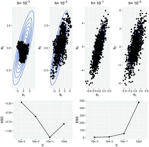We consider a range of step size parameters $h=\{{10}^{-3},{10}^{-2},{10}^{-1},{10}^0\}$ which satisfy the requirement that $h<4{\sigma }_2^2$ to prevent divergent chains. In Figure 1, we plot the samples generated from the Langevin algorithm for each of the step size parameters. We also calculate the kernel Stein discrepancy (13) and effective sample size for each Markov chain. Visually, it is clear from Figure 1 that h = 0.1 produces samples which most closely represent the target distribution. A large value for h leads to over-dispersed samples and a small h prevents the sampler from exploring the whole target space within the fixed number of iterations. Setting h = 0.1 also gives the lowest kernel Stein discrepancy, whereas h = 1 maximizes the effective sample size. This supports the view that effective sample size and other standard MCMC metrics, which do not account for sample bias, are not appropriate diagnostic tools for SGMCMC.

Fig. 1 Top: Samples generated from the Langevin dynamics (7) are plotted over the bivariate Gaussian target. The samples are thinned to 1000 for the ease of visualization. Bottom: The kernel Stein discrepancy (log10) and effective sample size are calculated for each Markov chain with varying step size parameter h.

5 Extending the SGMCMC Framework

Under the general SGMCMC framework outlined in Section 3, it is possible to extend the SGLD algorithm beyond Langevin dynamics and consider a larger class of MCMC algorithms, which aim to improve the mixing of the Markov chain. In this section, we will focus on ways to extend the applicability of SGMCMC algorithms to a wider class of models. Given our choice of target (1), we have made two key assumptions, (i) the parameters exist in $\mathit{\theta }\in {\mathbb{R}}^d$ and (ii) the potential function $U(\mathit{\theta })$ is a summation over independent terms. The first assumption implies that SGMCMC cannot be used to estimate $\mathit{\theta }$ on a constrained space (e.g., $\mathit{\theta }\in [0,1]$) and the second assumption that our data $y_1,\dots ,y_N$ are independent or have only certain-types of dependence structure, which means that SGMCMC cannot be applied to many time series or spatial models. We will give a short overview of some of the current research in this area.

5.1 SGMCMC Sampling From Constrained Spaces

Many models contain parameters which are constrained, for example, the variance parameter ${\tau }^2$ in a Gaussian distribution ($\tau \in {\mathbb{R}}^{+}$), or the success probability p in a Bernoulli model ($p\in [0,1]$). Simulating these constrained parameters using the Langevin dynamics (3) will produce samples which violate their constraints, for example, if ${\tau }_t^2={\mathit{\theta }}_t\gtrsim 0$, then with high probability, ${\tau }_{t+1}^2<0$. One solution would be to let $h\to 0$ when ${\tau }^2\to 0$, however, this would lead to poor mixing of the Markov chain near the boundary of the constrained space. A natural solution to this problem is to transform the Langevin dynamics in such a way that sampling can take place on the unconstrained space, but care is needed as the choice of transformation can impact the mixing of the process near the boundary. Alternatively we can project the Langevin dynamics into a constrained space (Brosse et al. 2017; Bubeck, Eldan, and Lehec 2018), however, these approaches lead to poorer nonasymptotic convergence rates than in the unconstrained setting. Recently, a mirrored Langevin algorithm (Hsieh et al. 2018) has been proposed, which builds on the mirrored descent algorithm (Beck and Teboulle 2003), to transform the problem of constrained sampling to an unconstrained space via a mirror mapping. Unlike previous works, the mirrored Langevin algorithm has convergence rates comparable with unconstrained SGLD (Dalalyan and Karagulyan 2019).

The structure of some models naturally leads to bespoke sampling strategies. A popular model in the machine learning literature is the latent Dirichlet allocation (LDA) model (Blei, Ng, and Jordan 2003), where the model parameters are constrained to the probability simplex, meaning ${\mathit{\theta }}^{(j)}\ge 0,j=1,\dots ,d$ and ${\sum }_{j=1}^d{\mathit{\theta }}^{(j)}=1$. Patterson and Teh (2013) proposed the first SGLD algorithm for sampling from the probability simplex. Their algorithm, stochastic gradient Riemannian Langevin dynamics (see Table 1) allows for several transformation schemes which transform $\mathit{\theta }$ to ${\mathbb{R}}^d$. However, this approach can result in asymptotic biases which dominate in the boundary regions of the constrained space. An alternative approach is to use the fact that the posterior for the LDA can be written as a transformation of independent gamma random variables. Using an alternative stochastic process instead of the Langevin diffusion, in this case the Cox–Ingersoll–Ross (CIR) process, we take advantage of the fact that its invariant distribution is a gamma distribution. We can apply this in the large data setting by using data subsampling on the CIR process rather than on the Langevin diffusion (Baker et al. 2018).

5.2 SGMCMC Sampling With Dependent Data

Key to developing SGMCMC algorithms is the ability to generate unbiased estimates of $\nabla U(\mathit{\theta })$ using data subsampling, as in (4). Under the assumption that data $y_i,i=1,\dots ,N$ are independent, the potential function $U(\mathit{\theta })={\sum }_{i=1}^N{U}_i(\mathit{\theta })$, and its derivative, are a sum of independent terms (see Section 2.1) and therefore, a random subsample of these terms leads to an unbiased estimate of the potential function, and its derivative. For some dependence structures, we can still write the potential as a sum of terms each of which has an O(1) cost to evaluate. However for many models used for network data, time series and spatial data, using the same random subsampling approach will result in biased estimates for $U(\mathit{\theta })$ and $\nabla U(\mathit{\theta })$. To the best of our knowledge, the challenge of subsampling spatial data, such that both short and long term dependency is captured, has not been addressed in the SGMCMC setting. For network data, an SGMCMC algorithm has been developed (Li, Ahn, and Welling 2016) for the mixed-member stochastic block model, which uses both the block structure of the model, and stratified subsampling techniques, to give unbiased gradient estimates.

In the time series setting, hidden Markov models are challenging for SGMCMC as the temporal dependence in the latent process precludes simple random data subsampling. However, such dependencies are often short range and so data points y_i and y_j will be approximately independent if they are sufficiently distant (i.e., $j\gg i$). These properties were used by Ma, Foti, and Fox (2017), who proposed using SGMCMC with gradients estimated using nonoverlapping, subsequences of length $2s+1,{\mathbf{y}}_{i,s}=\{y_{i-s},\dots ,y_i,\dots ,y_{i+s}\}$. To ensure that the subsequences are independent, Ma, Foti, and Fox (2017) extended the length of each subsequence by adding a buffer of size B, to either side, that is, $\{{\mathbf{y}}_{LB},{\mathbf{y}}_{i,s},{\mathbf{y}}_{RB}\}$, where ${\mathbf{y}}_{LB}=\{y_{i-s-B},\dots ,y_{i-s-1}\}$ and ${\mathbf{y}}_{RB}=\{y_{i+s+1},\dots ,y_{i+s+B}\}$. Nonoverlapping buffered subsequences are sampled, but only ${\mathbf{y}}_{i,s}$ data are used to estimate $\widehat{\nabla }U(\mathit{\theta })$. These methods introduce a bias, but one that can be controlled, with the bias often decreasing exponentially with the buffer size. This approach has also been applied to linear (Aicher et al. 2019) and nonlinear (Aicher et al. 2019) state-space models, where in the case of log-concave models, the bias decays geometrically with buffer size.

6 Simulation Study

We compare empirically the accuracy and efficiency of the SGMCMC algorithms described in Section 3. We consider three popular models. First, a logistic regression model for binary data classification tested on simulated data. Second, a Bayesian neural network (Neal 2012) applied to image classification on a popular dataset from the machine learning literature. Finally, we consider the Bayesian probabilistic matrix factorization (BPMF) model (Salakhutdinov and Mnih 2008) for predicting movie recommendations based on the MovieLens dataset. We compare the various SGMCMC algorithms against the STAN software (Carpenter et al. 2017), which by default implements the NUTS algorithm (Hoffman and Gelman 2014) as a method for automatically tuning the Hamiltonian MCMC sampler. We treat the STAN output as the ground truth posterior distribution and assess the accuracy and computational advantages of SGMCMC against this benchmark. Additionally, using STAN, we can sample from a variational approximation to the posterior using the automatic differentiation variational inference (ADVI) algorithm (Kucukelbir et al. 2015), which selects an appropriate variational family and optimizes the corresponding variational objective. All of the SGMCMC algorithms are implemented using the R package sgmcmc (Baker et al. 2019b) with supporting code available online.¹

6.1 Logistic Regression Model

Consider a binary regression model where $\mathbf{y}={\left\{y_i\right\}}_{i=1}^N$ is a vector of N binary responses and X is a N × d matrix of covariates. If $\mathit{\theta }$ is a d-dimensional vector of model parameters, then the likelihood function for the logistic regression model is,$$p(\mathbf{y},\mathbf{X}|\mathit{\theta })=\prod _{i=1}^N{\left[\frac{1}{1+\hspace{0.17em}\text{exp}\hspace{0.17em}(-{\mathit{\theta }}^{\top }{\mathbf{x}}_i)}\right]}^{y_i}{\left[1-\frac{1}{1+\hspace{0.17em}\text{exp}\hspace{0.17em}(-{\mathit{\theta }}^{\top }{\mathbf{x}}_i)}\right]}^{1-y_i},$$where ${\mathbf{x}}_i$ is a d-dimensional vector for the ith observation. The prior distribution for $\mathit{\theta }$ is a zero-mean Gaussian with covariance matrix ${\mathbf{\Sigma }}_{\mathit{\theta }}=10{\mathbf{I}}_d$, where ${\mathbf{I}}_d$ is a d × d identity matrix. We can verify that the model satisfies the strong-convexity assumptions from Section 2.4, where $m={\lambda }_{\text{max}}^{-1}({\mathbf{\Sigma }}_{\mathit{\theta }})$ and $M=\frac{1}{4}{\sum }_{i=1}^N{\mathbf{x}}_i^{\top }{\mathbf{x}}_i+{\lambda }_{\text{min}}^{-1}({\mathbf{\Sigma }}_{\mathit{\theta }})$, and ${\lambda }_{\text{min}}({\mathbf{\Sigma }}_{\mathit{\theta }})$ and ${\lambda }_{\text{max}}({\mathbf{\Sigma }}_{\mathit{\theta }})$ are the minimum and maximum eigenvalues of ${\mathbf{\Sigma }}_{\mathit{\theta }}$.

We compare the various SGMCMC algorithms where we vary the dimension of $\mathit{\theta },d=\{10,50,100\}$. We simulate $N={10}^5$ data points and fix the subsample size $n=0.01N$ for all test cases. We simulated data under the model described above, with ${\mathbf{x}}_i\sim N(0,{\mathbf{\Sigma }}_{\mathbf{x}})$ and simulated a matrix with ${\mathbf{\Sigma }}_{\mathbf{x}}^{(i,j)}=\text{Unif}{[-\rho ,\rho ]}^{|i-j|}$ and $\rho =0.4$. We tune the step size h for each algorithm using the kernel Stein discrepancy metric outlined in Section 4 and set the number of leapfrog steps in SGHMC to five. We initialize each sampler by randomly sampling the first iteration ${\mathit{\theta }}_0\sim N(0,1)$.

For our simulations, we ran STAN for 2000 iterations and discarded the first 1000 iterations as burn-in, as these iterations are part of the algorithms tuning phase. For the SGMCMC algorithms, we ran each algorithm for 20,000 iterations except in the case of the control variate implementations, where we ran the SGMCMC algorithm for 10,000 iterations after iterating a SGD algorithm for 10,000 iterations to find the posterior mode $\widehat{\mathit{\theta }}$. Combining the optimization and sampling steps of the control variate method results in an equal number of iterations for all SGMCMC algorithms. Figure 2 gives the trace plots for MCMC output of each algorithm for the case where d = 10 and $N={10}^5$. Each of the SGMCMC algorithms is initialized with the same ${\mathit{\theta }}_0$ and we see that some components of $\mathit{\theta }$, where the posterior is not concentrated around ${\mathit{\theta }}_0$, take several thousand iterations to converge. Most notably SGLD, ULA, SGHMC, and SGNHT. Of these algorithms, SGHMC and SGNHT converge faster than SGLD, which reflects the theoretical results discussed in Section 3.1, but these algorithms also have a higher computational cost due to the leap frog steps (see Table 2 for computational timings). The ULA algorithm, which uses exact gradients, also converges faster than SGLD in terms of the number of iterations, but is less efficient in terms of overall computational time. The control variate SGMCMC algorithms, SGLD-CV, SGHMC-CV, and SGNHT-CV are all more efficient than their noncontrol variate counterparts in terms of the number of iterations required for convergence. The control variate algorithms have the advantage that their sampling phase is initialized at a ${\mathit{\theta }}_0$ that is close to the posterior mode. In essence, the optimization phase required to find the control variate point $\widehat{\mathit{\theta }}$ replaces the burn-in phase of the Markov chain for the SGMCMC algorithm.

Fig. 2 Trace plots for the STAN output and each SGMCMC algorithm with d = 10 and $N={10}^5$.

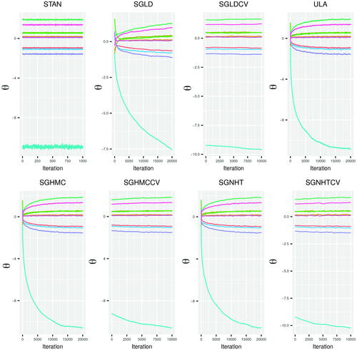
Table 2 Diagnostic metrics for each SGMCMC algorithm, plus STAN, with varying dimension of $\mathit{\theta }$ where $N={10}^5$.

	d	STAN	SGLD	SGLDCV	SGHMC	SGHMCCV	SGNHT	SGNHTCV	ULA	ADVI
Time (min)	10	21.64	1.74	1.46	11.24	6.53	2.56	1.54	8.05	0.76
	50	157.24	2.55	2.06	13.43	7.76	3.33	1.93	29.21	2.37
	100	229.76	3.42	2.60	16.01	9.63	4.38	2.36	51.25	4.15
Log-loss	10	0.10	0.11	0.10	0.10	0.10	0.10	0.10	0.10	0.10
	50	0.04	0.06	0.05	0.06	0.05	0.05	0.05	0.05	0.07
	100	0.04	0.06	0.05	0.06	0.05	0.05	0.05	0.06	0.07
KSD	10	6.12	6.26	6.24	6.18	6.25	6.21	6.23	6.19	6.97
	50	9.24	11.73	11.05	11.59	11.11	11.00	11.33	11.30	11.66
	100	11.62	15.70	15.53	15.64	15.07	15.14	15.07	15.97	13.61

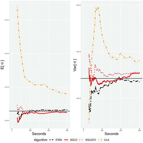
The results from Figure 2 are shown for a fixed number of iterations, however, the computational cost per iteration varies between the algorithms. In Figure 3, we run STAN, SGLD, SGLD-CV, and ULA for 10 min, treating the first minute as the burn-in phase and a longer 1-hr run of STAN as the truth. We can see in this experiment that over short time-periods SGLD performs well, whereas STAN underestimates the posterior variance due to fewer iterations, which results in less time for the chain to mix. SGLD and SGLD-CV produce good estimates of the mean, but as discussed in Section 2.5, SGLD and SGLD-CV over-estimate the variance. Using exact gradients with ULA performs poorly as it does not have the same gains in computational efficiency of SGLD and still has an approximation error.

Fig. 3 The mean and variance of the first parameter calculated at each second over 600 sec, where d = 10 and $N={10}^5$.

As well as the visual comparisons (Figure 2), we can compare the algorithms using diagnostic metrics. We use the kernel Stein discrepancy as one of the metrics to assess the quality of the posterior approximation for each of the algorithms. Additionally, the log-loss is also a popular metric for measuring the predictive accuracy of a classifier on a held-out test dataset $T_{*}$. In the case of predicted binary responses, the log-loss is$$\begin{array}{c}l(\mathit{\theta },T_{*})=-\frac{1}{\left|T_{*}\right|}\sum _{(y_{*},{\mathbf{x}}_{*})\in T_{*}}{y}_{*}\hspace{0.17em}\text{log}\hspace{0.17em}p({\mathbf{x}}_{*},\mathit{\theta })\\ \hspace{1em}+(1-y_{*})\hspace{0.17em}\text{log}\hspace{0.17em}(1-p({\mathbf{x}}_{*},\mathit{\theta })),\end{array}$$where $p({\mathbf{x}}_{*},\mathit{\theta })={(1+\hspace{0.17em}\text{exp}\hspace{0.17em}(-{\mathit{\theta }}^{\top }{\mathbf{x}}_{*}))}^{-1}$ is the probability that $y_{*}=1$ given covariate ${\mathbf{x}}_{*}$.

Table 2 gives the diagnostic metrics for each algorithm, where the log-loss and kernel Stein discrepancy metrics are calculated on the final 1000 posterior samples from each algorithm. We also include a variational Bayes approximation using STAN’s ADVI algorithm. The variational Bayes approaches are generally faster than MCMC as they use optimization techniques rather than sampling to approximate the posterior. These variational techniques work particularly well when the posterior is close to its approximating family of distributions, which are usually assumed to be Gaussian. The most notable difference between the algorithms is the computational time. Compared to STAN, all SGMCMC algorithms, and ADVI, are between 10 to 100 times faster when d = 100. As expected, given that STAN produces exact posterior samples, it has the lowest log-loss and kernel Stein discrepancy results. However, these results are only slightly better than the SGMCMC results and the computational cost of STAN is significantly higher. All of the SGMCMC results are similar, showing that this class of algorithms can perform well, with significant computational savings, if they are well-tuned. Similarly, we note that the variational approximations produce accuracy results similar to SGMCMC and are significantly computationally cheaper than STAN. One of the advantages of STAN, is that the NUTS algorithm (Hoffman and Gelman 2014) allows the HMC sampler to be automatically tuned, whereas the SGMCMC algorithms have to be tuned using a pilot run over a grid of step size values. As the step size h is a scalar value, the SGMCMC samplers give an equal step size to each dimension. As discussed in Section 2.5, a scalar step size parameter will mean that the SGMCMC algorithms are constrained by the $\mathit{\theta }$ component with the smallest variance. This could be improved if either the gradients were preconditioned (Ahn, Korattikara, and Welling 2012), or the geometry of the posterior space were accounted for in the sampler (e.g., SGRHMC), which would result in different step sizes for each component of $\mathit{\theta }$, thus improving the overall efficiency of the sampler.

6.2 Bayesian Neural Network

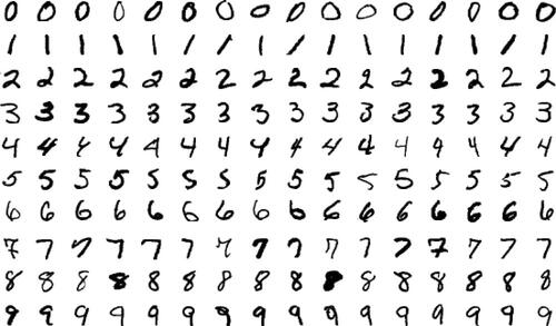
We consider the problem of multi-class classification on the popular MNIST dataset (LeCun, Cortes, and Burges 2010). The MNIST dataset consists of a collection of images of handwritten digits from zero to nine, where each image is represented as 28 × 28 pixels (a sample of images is shown in Figure 4). We model the data using a two layer Bayesian neural network with 100 hidden variables (using the same setup as Chen, Fox, and Guestrin (2014)). We fit the neural network to a training dataset containing 55,000 images and the goal is to classify new images as belonging to one of the ten categories. The test set contains 10,000 handwritten images, with corresponding labels.

Fig. 4 Sample of images from the MNIST dataset taken from https://en.wikipedia.org/wiki/MNIST/_database.

Let y_i be the image label taking values $y_i\in \{0,1,2,3,4,5,6,7,8,9\}$ and ${\mathbf{x}}_i$ is the vector of pixels which has been flattened from a 28 × 28 image to a one-dimensional vector of length 784. If there are N training images, then $\mathbf{X}$ is a $N\times 784$ matrix representing the full dataset of pixels. We model the data as categorical variables with the probability mass function,(14) $$p(y_i=k|\mathit{\theta },{\mathbf{x}}_i)={\beta }_k(\mathit{\theta },{\mathbf{x}}_i),$$(14) where ${\beta }_k(\mathit{\theta },{\mathbf{x}}_i)$ is the kth element of $\beta (\mathit{\theta },{\mathbf{x}}_i)=\sigma (\sigma ({\mathbf{x}}_i^{\top }B+b)A+a)$ and $\sigma ({\mathbf{x}}_i)=\hspace{0.17em}\text{exp}\hspace{0.17em}({\mathbf{x}}_i)/({\sum }_{j=1}^N\hspace{0.17em}\text{exp}\hspace{0.17em}({\mathbf{x}}_i))$ is the softmax function, a generalization of the logistic link function. The parameters $\mathit{\theta }=(A,B,a,b)$ will be estimated using SGMCMC, where A, B, a, and b are matrices of dimension: 100 × 10, 784 × 100, 1 × 10, and 1 × 100, respectively. We set normal priors for each element of these parameters$$\begin{array}{c}{A}_{kl}|{\lambda }_A\sim N(0,{\lambda }_A^{-1}),\mathrm{\hspace{1em}}\mathrm{\hspace{1em}}{B}_{jk}|{\lambda }_B\sim N(0,{\lambda }_B^{-1}),\\ a_l|{\lambda }_a\sim N(0,{\lambda }_a^{-1}),\mathrm{\hspace{1em}}\mathrm{\hspace{1em}}{b}_k|{\lambda }_b\sim N(0,{\lambda }_b^{-1}),\end{array}$$ $j=1,\dots ,784;k=1,\dots ,100;l=1,\dots ,10;$ where ${\lambda }_A,{\lambda }_B,{\lambda }_a,{\lambda }_b\sim \text{Gamma}(1,1)$ are hyperparameters.

Similar to the logistic regression example (see Section 6.1), we use the log-loss as a test function. We need to update the definition of the log-loss function from a binary classification problem to the multi-class setting. Given a test set $T_{*}$ of pairs $(y_{*},{\mathbf{x}}_{*})$, where now $y_{*}$ can take values $\{0-9\}$. The log-loss function in the multi-class setting is now(15) $$l(\mathit{\theta },T_{*})=-\frac{1}{\left|T_{*}\right|}\sum _{(y_{*},{\mathbf{x}}_{*})\in T_{*}}\sum _{k=0}^9{1}_{y_{*}=k}\hspace{0.17em}\text{log}\hspace{0.17em}{\beta }_k(\mathit{\theta },{\mathbf{x}}_{*}),$$(15) where $1_A$ is the indicator function, and ${\beta }_k(\mathit{\theta },{\mathbf{x}}_{*})$ is the kth element of $\beta (\mathit{\theta },{\mathbf{x}}_{*})$.

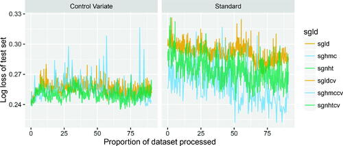
As in Section 6.1, we compare the efficacy of the SGLD, SGHMC, and SGNHT algorithms, as well as their control variate counterparts. We ran each of the SGMCMC algorithms for 10⁴ iterations and calculated the log-loss (14) for each algorithm. The standard algorithms have 10⁴ iterations of burn-in while the control variate algorithms have no burn-in, but 10⁴ iterations in the initial optimization step. Note that due to the trajectory parameter L = 5 of SGHMC and SGHMC-CV, these algorithms will have approximately five times greater computational cost. To balance the computational cost, we ran these algorithms for 2000 iterations to produce comparisons with approximately equal computational time. The results are plotted in Figure 5. As with the logistic regression example, we note that there is some indication of improved predictive performance of the control variate methods. Among the standard methods, SGHMC and SGNHT have the best predictive performance, which is to be expected given the apparent trade-off between accuracy and exploration.

Fig. 5 Log-loss calculated on a held-out test dataset for each SGMCMC algorithm and its control variate version.

6.3 Bayesian Probabilistic Matrix Factorization

Collaborative filtering is a technique used in recommendation systems to make predictions about a user’s interests based on their tastes and preferences. We can represent these preferences with a matrix where the (i, j)th entry is the score that user i gives to item j. This matrix is naturally sparse as not all users provide scores for all items. We can model these data using BPMF (Salakhutdinov and Mnih 2008), where the preference matrix of user-item ratings is factorized into lower-dimensional matrices representing the users’ and items’ latent features. A popular application of BPMF is movie recommendations, where the preference matrix contains the ratings for each movie given by each user. This model has been successfully applied to the Netflix dataset to extract the latent user-item features from the historical data to make movie recommendations for a held-out test set of users. In this example, we will consider the MovieLens dataset² which contains 100,000 ratings (taking values $\{1,2,3,4,5\}$) of 1682 movies by 943 users, where each user has provided at least 20 ratings. The data are already split into 5 training and test sets ($80\%/20\%$ split) for a 5-fold cross-validation experiment.

Let $\mathbf{R}\in {\mathbb{R}}^{N\times M}$ be a matrix of observed ratings for N users and M movies where R_ij is the rating user i gave to movie j. We introduce matrices U and V for users and movies, respectively, where ${\mathbf{U}}_i\in {\mathbb{R}}^d$ and ${\mathbf{V}}_j\in {\mathbb{R}}^d$ are d-dimensional latent feature vectors for user i and movie j. The likelihood for the rating matrix is$$p(\mathbf{R}|\mathbf{U},\mathbf{V},\alpha )=\prod _{i=1}^N\prod _{j=1}^M{\left[N(R_{ij}|{\mathbf{U}}_i^{\top }{\mathbf{V}}_j,{\alpha }^{-1})\right]}^{I_{ij}},$$where I_ij is an indicator variable which equals 1 if user i gave a rating for movie j. The prior distributions for the users and movies are$$\begin{array}{c}p(\mathbf{U}|{\mu }_{\mathbf{U}},{\Lambda }_{\mathbf{U}})=\prod _{i=1}^{N}N({\mathbf{U}}_i|{\mu }_{\mathbf{U}},{\Lambda }_{\mathbf{U}}^{-1})\hspace{1em}\text{and}\\ p(\mathbf{V}|{\mu }_{\mathbf{V}},{\Lambda }_{\mathbf{V}})=\prod _{j=1}^{M}N({\mathbf{V}}_j|{\mu }_{\mathbf{V}},{\Lambda }_{\mathbf{V}}^{-1}),\end{array}$$ with prior distributions on the hyperparameters (where $\mathbf{W}=\mathbf{U}$ or V) given by,$${\mu }_{\mathbf{W}}\sim N({\mu }_{\mathbf{W}}|{\mu }_0,{\Lambda }_{\mathbf{W}})\text{and}{\Lambda }_{\mathbf{W}}\sim \text{Gamma}(a_0,b_0).$$

The parameters of interest in our model are then $\mathit{\theta }=(\mathbf{U},{\mu }_{\mathbf{U}},{\Lambda }_{\mathbf{U}},\mathbf{V},{\mu }_{\mathbf{V}},{\Lambda }_{\mathbf{V}})$ and the hyperparameters for the experiments are $\mathit{\tau }=(\alpha ,{\mu }_0,a_0,b_0)=(3,0,1,5)$. We are free to choose the size of the latent dimension and for these experiments we set d = 20.

The predictive distribution for an unknown rating $R_{ij}^{*}$ given to movie j by user i, is found by marginalizing over the latent feature parameters$$p(R_{ij}^{*}|\mathbf{R},\mathit{\tau })=\int p(R_{ij}^{*}|{\mathbf{U}}_i,{\mathbf{V}}_j,\alpha )\pi (\mathit{\theta }|\mathbf{R},\mathit{\tau })\mathrm{d}\mathit{\theta }.$$

We can approximate the predictive density using Monte Carlo integration, where the posterior samples, conditional on the training data, are generated using the SGMCMC algorithms. The held-out test data can be used to assess the predictive accuracy of each of the SGMCMC algorithms, where we use the root mean square error (RMSE) between the predicted and actual rating as an accuracy metric.

We ran each of the SGMCMC algorithms for 10⁵ iterations, where for SGLD-CV and SGHMC-CV we applied a SGD algorithm for 50,000 iterations to find the posterior mode and used this as the fixed point for the control variate, as well as initializing these SGMCMC samplers from the control variate point (i.e., ${\mathit{\theta }}_0=\widehat{\mathit{\theta }}$). 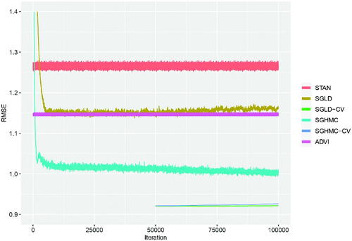Given the size of the parameter space, we increase the subsample size to $n=0.1N$ per iteration and tune the step size parameter for each SGMCMC algorithm using diagnostic tests (see Section 4) on a pilot run with 10⁴ iterations. As a baseline to assess the accuracy of the SGMCMC algorithms we applied the NUTS sampler from the STAN software to the full dataset and ran this for 10⁴ iterations, discarding the first half as burn-in. We also tested a fast variational approximation using STAN’s ADVI algorithm. Figure 6 gives the RMSE for STAN, ADVI, SGLD, and SGHMC along with their control variate versions. The results show that SGHMC produces a lower RMSE than SGLD on the test data with equally improved results for their control variate implementations. ADVI, SGLD, and SGHMC quickly converge to a stable RMSE after a few thousand iterations with SGLD-CV and SGHMC-CV producing an overall lower RMSE immediately as they are both initialized from the posterior mode, which removes the burn-in phase. Most notable from these results is that all of the SGMCMC algorithms, and ADVI, outperform the STAN baseline RMSE. The poorer performance of STAN is attributable to running the algorithm for fewer iterations than the SGMCMC algorithms which could mean that the MCMC sampler has not converged. Running STAN for 10% of the iterations of the SGMCMC algorithms took 3.5 days, whereas SGLD, SGLD-CV, SGHMC, and SGHMC-CV took 3.1, 1.9, 16.4, and 14.8 hr, respectively. The ADVI algorithm has a similar computational time to the SGMCMC algorithms, but as it is an optimization rather than sampling routine, the algorithm stops after it has converged, which in this example occurs after approximately 1000 iterations. Overall, while SGMCMC algorithms produce biased posterior approximations compared to exact MCMC algorithms, such as STAN’s NUTS sampler, they can produce accurate estimates of quantities of interest at significantly reduced computational cost.

Fig. 6 Root mean square error on the predictive performance of each SGMCMC algorithm averaged over five cross-validation experiments.

7 Discussion

In this article, we have provided a review of the growing literature on SGMCMC algorithms. These algorithms utilize data subsampling to significantly reduce the computational cost of MCMC. As shown in this article, these algorithms are theoretically well-understood and provide parameter inference at levels of accuracy that are comparable to traditional MCMC algorithms. SGMCMC is still a relatively new class of Monte Carlo algorithms compared to traditional MCMC methods and there remain many open problems and opportunities for further research in this area.

Some key areas for future development in SGMCMC include:

• New algorithms—as discussed in Section 3.1, SGMCMC represents a general class of scalable MCMC algorithms with many popular algorithms given as special cases, therefore, it is possible to derive new algorithms from this general setting which may be more applicable for certain types of target distribution.

• General theoretical results—most of the current theoretical results which bound the error of SGMCMC algorithms assume that the target distribution is log-concave. Relaxing this assumption is nontrivial and may need completely different arguments to show similar nonasymptotic error bounds for a broader class of models.

• Tuning techniques—as outlined in Section 4, the efficacy of SGMCMC is dependent on how well the step size parameter is tuned. Standard MCMC tuning rules, such as those based on acceptance rates, are not applicable and new techniques, such as the Stein discrepancy metrics, can be computationally expensive to apply. Developing robust tuning rules, which can be applied in an automated fashion, would make it easier for nonexperts to use SGMCMC methods in the same way that adaptive HMC has been applied in the STAN software.

A major success of traditional MCMC algorithms, and their broad appeal in a range of application areas, is partly a result of freely available software, such as WinBUGS (Lunn et al. 2000), JAGS (Plummer 2003), NIMBLE (de Valpine et al. 2017), and STAN (Carpenter et al. 2017). Open-source MCMC software, which may utilize specials features of the target distribution, or provide automatic techniques to adapt the tuning parameters, make MCMC methods more user-friendly to general practitioners. Similar levels of development for SGMCMC, which provide automatic differentiation and adaptive step size parameter tuning, would help lower the entry level for nonexperts. Some recent developments in this area include sgmcmc in R (Baker et al. 2019b) and Edward in Python (Tran et al. 2016), but further development is required to fully utilize the general SGMCMC framework.

Acknowledgments

The authors would like to thank Jack Baker for his guidance and help using the sgmcmc package.

Supplementary Materials

Supplementary materials are available, which include the R code from Section 6. Code can also be found online at https://github.com/chris-nemeth/sgmcmc-review-paper.

Additional information

Funding

CN gratefully acknowledges the support of EPSRC grants EP/S00159X/1 and EP/R01860X/1. PF is supported by the EPSRC-funded projects Bayes4Health EP/R018561/1 and CoSInES EP/R034710/1.

Notes

1 https://github.com/***

2 https://grouplens.org/datasets/movielens/100k/

References

- Ahn, S., Korattikara, A., Liu, N., Rajan, S., and Welling, M. (2015), “Large-Scale Distributed Bayesian Matrix Factorization Using Stochastic Gradient MCMC,” in Proceedings of the 21th ACM SIGKDD International Conference on Knowledge Discovery and Data Mining, ACM, pp. 9–18. DOI: 10.1145/2783258.2783373.
- Ahn, S., Korattikara, A., and Welling, M. (2012), “Bayesian Posterior Sampling via Stochastic Gradient Fisher Scoring,” in Proceedings of the 29th International Conference on Machine Learning, ICML 2012, pp. 1591–1598.
- Aicher, C., Ma, Y.-A., Foti, N. J., and Fox, E. B. (2019), “Stochastic Gradient MCMC for State Space Models,” SIAM Journal on Mathematics of Data Science, 1, 555–587. DOI: 10.1137/18M1214780.
- Aicher, C., Putcha, S., Nemeth, C., Fearnhead, P., and Fox, E. B. (2019), “Stochastic Gradient MCMC for Nonlinear State Space Models,” arXiv no. 1901.10568.
- Andersen, M., Winther, O., Hansen, L. K., Poldrack, R., and Koyejo, O. (2018), “Bayesian Structure Learning for Dynamic Brain Connectivity,” in International Conference on Artificial Intelligence and Statistics, pp. 1436–1446.
- Baker, J., Fearnhead, P., Fox, E. B., and Nemeth, C. (2018), “Large-Scale Stochastic Sampling From the Probability Simplex,” in Advances in Neural Information Processing Systems, pp. 6721–6731.
- Baker, J., Fearnhead, P., Fox, E. B., and Nemeth, C. (2019a), “Control Variates for Stochastic Gradient MCMC,” Statistics and Computing, 29, 599–615.
- Baker, J., Fearnhead, P., Fox, E. B., and Nemeth, C. (2019b), “sgmcmc: An R Package for Stochastic Gradient Markov Chain Monte Carlo,” Journal of Statistical Software, 91, 1–27.
- Balan, A. K., Rathod, V., Murphy, K. P., and Welling, M. (2015), “Bayesian Dark Knowledge,” in Advances in Neural Information Processing Systems, pp. 3438–3446.
- Bardenet, R., Doucet, A., and Holmes, C. (2014), “Towards Scaling Up Markov Chain Monte Carlo: An Adaptive Subsampling Approach,” in International Conference on Machine Learning (ICML), pp. 405–413.
- Bardenet, R., Doucet, A., and Holmes, C. (2017), “On Markov Chain Monte Carlo Methods for Tall Data,” The Journal of Machine Learning Research, 18, 1515–1557.
- Beck, A., and Teboulle, M. (2003), “Mirror Descent and Nonlinear Projected Subgradient Methods for Convex Optimization,” Operations Research Letters, 31, 167–175. DOI: 10.1016/S0167-6377(02)00231-6.
- Besag, J. (1994), “Comments on ‘Representations of Knowledge in Complex Systems’ by U. Grenander and MI Miller,” Journal of the Royal Statistical Society, Series B, 56, 591–592.
- Bierkens, J., Fearnhead, P., and Roberts, G. O. (2019), “The Zig-Zag Process and Super-Efficient Sampling for Bayesian Analysis of Big Data,” The Annals of Statistics, 47, 1288–1320. DOI: 10.1214/18-AOS1715.
- Bishop, C. M. (2006), Pattern Recognition and Machine Learning, New York: Springer.
- Blei, D. M., Kucukelbir, A., and McAuliffe, J. D. (2017), “Variational Inference: A Review for Statisticians,” Journal of the American Statistical Association, 112, 859–877. DOI: 10.1080/01621459.2017.1285773.
- Blei, D. M., Ng, A. Y., and Jordan, M. I. (2003), “Latent Dirichlet Allocation,” Journal of Machine Learning Research, 3, 993–1022.
- Bouchard-Côté, A., Vollmer, S. J., and Doucet, A. (2018), “The Bouncy Particle Sampler: A Nonreversible Rejection-Free Markov Chain Monte Carlo Method,” Journal of the American Statistical Association, 113, 855–867. DOI: 10.1080/01621459.2017.1294075.
- Brooks, S., and Gelman, A. (1998), “General Methods for Monitoring Convergence of Iterative Simulations,” Journal of Computational and Graphical Statistics, 7, 434–455.
- Brooks, S., Gelman, A., Jones, G., and Meng, X.-L. (2011), Handbook of Markov Chain Monte Carlo, Boca Raton, FL: CRC Press.
- Brosse, N., Durmus, A., and Moulines, É. (2018), “The Promises and Pitfalls of Stochastic Gradient Langevin Dynamics,” in Advances in Neural Information Processing Systems, pp. 8278–8288.
- Brosse, N., Durmus, A., Moulines, É., and Pereyra, M. (2017), “Sampling From a Log-Concave Distribution With Compact Support With Proximal Langevin Monte Carlo,” in Conference on Learning Theory, pp. 319–342.
- Bubeck, S., Eldan, R., and Lehec, J. (2018), “Sampling From a Log-Concave Distribution With Projected Langevin Monte Carlo,” Discrete & Computational Geometry, 59, 757–783.
- Carpenter, B., Gelman, A., Hoffman, M. D., Lee, D., Goodrich, B., Betancourt, M., Brubaker, M., Guo, J., Li, P., and Riddell, A. (2017), “Stan: A Probabilistic Programming Language,” Journal of Statistical Software, 76, 1–32. DOI: 10.18637/jss.v076.i01.
- Chatterji, N., Flammarion, N., Ma, Y., Bartlett, P., and Jordan, M. (2018), “On the Theory of Variance Reduction for Stochastic Gradient Monte Carlo,” in Proceedings of Machine Learning Research (PMLR) (Vol. 80), pp. 764–773.
- Chen, T., Fox, E., and Guestrin, C. (2014), “Stochastic Gradient Hamiltonian Monte Carlo,” in International Conference on Machine Learning, pp. 1683–1691.
- Cheng, X., Chatterji, N. S., Bartlett, P. L., and Jordan, M. I. (2018), “Underdamped Langevin MCMC: A Non-Asymptotic Analysis,” in Proceedings of the 31st Conference on Learning Theory, Proceedings of Machine Learning Research (PMLR), eds. S. Bubeck, V. Perchet, and P. Rigollet, pp. 300–323.
- Dalalyan, A. S. (2017), “Theoretical Guarantees for Approximate Sampling From Smooth and Log-Concave Densities,” Journal of the Royal Statistical Society, Series B, 79, 651–676. DOI: 10.1111/rssb.12183.
- Dalalyan, A. S., and Karagulyan, A. (2019), “User-Friendly Guarantees for the Langevin Monte Carlo With Inaccurate Gradient,” Stochastic Processes and Their Applications, 129, 5278–5311. DOI: 10.1016/j.spa.2019.02.016.
- de Valpine, P., Turek, D., Paciorek, C. J., Anderson-Bergman, C., Lang, D. T., and Bodik, R. (2017), “Programming With Models: Writing Statistical Algorithms for General Model Structures With Nimble,” Journal of Computational and Graphical Statistics, 26, 403–413. DOI: 10.1080/10618600.2016.1172487.
- Ding, N., Fang, Y., Babbush, R., Chen, C., Skeel, R. D., and Neven, H. (2014), “Bayesian Sampling Using Stochastic Gradient Thermostats,” in Advances in Neural Information Processing Systems, pp. 3203–3211.
- Dubey, K. A., Reddi, S. J., Williamson, S. A., Poczos, B., Smola, A. J., and Xing, E. P. (2016), “Variance Reduction in Stochastic Gradient Langevin Dynamics,” in Advances in Neural Information Processing Systems, pp. 1154–1162.
- Dunson, D. B., and Johndrow, J. (2020), “The Hastings Algorithm at Fifty,” Biometrika, 107, 1–23. DOI: 10.1093/biomet/asz066.
- Durmus, A., and Moulines, E. (2017), “Nonasymptotic Convergence Analysis for the Unadjusted Langevin Algorithm,” The Annals of Applied Probability, 27, 1551–1587. DOI: 10.1214/16-AAP1238.
- Ermak, D. L. (1975), “A Computer Simulation of Charged Particles in Solution. I. Technique and Equilibrium Properties,” The Journal of Chemical Physics, 62, 4189–4196. DOI: 10.1063/1.430300.
- Fearnhead, P., Bierkens, J., Pollock, M., and Roberts, G. O. (2018), “Piecewise Deterministic Markov Processes for Continuous-Time Monte Carlo,” Statistical Science, 33, 386–412. DOI: 10.1214/18-STS648.
- Fearnhead, P., Papaspiliopoulos, O., and Roberts, G. O. (2008), “Particle Filters for Partially Observed Diffusions,” Journal of the Royal Statistical Society, Series B, 70, 755–777. DOI: 10.1111/j.1467-9868.2008.00661.x.
- Gan, Z., Chen, C., Henao, R., Carlson, D., and Carin, L. (2015), “Scalable Deep Poisson Factor Analysis for Topic Modeling,” in International Conference on Machine Learning, pp. 1823–1832.
- Gibbs, A. L., and Su, F. E. (2002), “On Choosing and Bounding Probability Metrics,” International Statistical Review, 70, 419–435. DOI: 10.1111/j.1751-5823.2002.tb00178.x.
- Girolami, M., and Calderhead, B. (2011), “Riemann Manifold Langevin and Hamiltonian Monte Carlo Methods” (with discussion), Journal of the Royal Statistical Society, Series B, 73, 123–214. DOI: 10.1111/j.1467-9868.2010.00765.x.
- Gorham, J., Duncan, A. B., Vollmer, S. J., and Mackey, L. (2019), “Measuring Sample Quality With Diffusions,” The Annals of Applied Probability, 29, 2884–2928. DOI: 10.1214/19-AAP1467.
- Gorham, J., and Mackey, L. (2015), “Measuring Sample Quality With Stein’s Method,” in Advances in Neural Information Processing Systems, pp. 226–234.
- Gorham, J., and Mackey, L. (2017), “Measuring Sample Quality With Kernels,” in Proceedings of the 34th International Conference on Machine Learning (Vol. 70), JMLR.org, pp. 1292–1301.
- Hastings, W. K. (1970), “Monte Carlo Sampling Methods Using Markov Chains and Their Applications,” Biometrika, 57, 97–109. DOI: 10.1093/biomet/57.1.97.
- Hoffman, M. D., and Gelman, A. (2014), “The No-U-Turn Sampler: Adaptively Setting Path Lengths in Hamiltonian Monte Carlo,” Journal of Machine Learning Research, 15, 1593–1623.
- Hsieh, Y.-P., Kavis, A., Rolland, P., and Cevher, V. (2018), “Mirrored Langevin Dynamics,” in Advances in Neural Information Processing Systems, pp. 2883–2892.
- Huggins, J., and Zou, J. (2017), “Quantifying the Accuracy of Approximate Diffusions and Markov Chains,” in Artificial Intelligence and Statistics, pp. 382–391.
- Korattikara, A., Chen, Y., and Welling, M. (2014), “Austerity in MCMC Land: Cutting the Metropolis–Hastings Budget,” in International Conference on Machine Learning, pp. 181–189.
- Kucukelbir, A., Ranganath, R., Gelman, A., and Blei, D. (2015), “Automatic Variational Inference in Stan,” in Advances in Neural Information Processing Systems, pp. 568–576.
- LeCun, Y., Cortes, C., and Burges, C. (2010), “MNIST Handwritten Digit Database,” AT&T Labs [online], available at http://yann.lecun.com/exdb/mnist.
- Li, W., Ahn, S., and Welling, M. (2016), “Scalable MCMC for Mixed Membership Stochastic Blockmodels,” in Artificial Intelligence and Statistics, pp. 723–731.
- Lunn, D. J., Thomas, A., Best, N., and Spiegelhalter, D. (2000), “WinBUGS—A Bayesian Modelling Framework: Concepts, Structure, and Extensibility,” Statistics and Computing, 10, 325–337. DOI: 10.1023/A:1008929526011.
- Ma, Y.-A., Chen, T., and Fox, E. (2015), “A Complete Recipe for Stochastic Gradient MCMC,” in Advances in Neural Information Processing Systems, pp. 2917–2925.
- Ma, Y.-A., Foti, N. J., and Fox, E. B. (2017), “Stochastic Gradient MCMC Methods for Hidden Markov Models,” arXiv no. 1706.04632.
- Majka, M. B., Mijatović, A., and Szpruch, Ł. (2020), “Nonasymptotic Bounds for Sampling Algorithms Without Log-Concavity,” The Annals of Applied Probability, 30, 1534–1581. DOI: 10.1214/19-AAP1535.
- Metropolis, N., Rosenbluth, A. W., Rosenbluth, M. N., Teller, A. H., and Teller, E. (1953), “Equation of State Calculations by Fast Computing Machines,” The Journal of Chemical Physics, 21, 1087–1092. DOI: 10.1063/1.1699114.
- Meyn, S. P., and Tweedie, R. L. (1994), “Computable Bounds for Geometric Convergence Rates of Markov Chains,” The Annals of Applied Probability, 4, 981–1011. DOI: 10.1214/aoap/1177004900.
- Minka, T. P. (2001), “Expectation Propagation for Approximate Bayesian Inference,” in Proceedings of the 17th Conference on Uncertainty in Artificial Intelligence, Morgan Kaufmann Publishers Inc., pp. 362–369.
- Minsker, S., Srivastava, S., Lin, L., and Dunson, D. B. (2017), “Robust and Scalable Bayes via a Median of Subset Posterior Measures,” The Journal of Machine Learning Research, 18, 4488–4527.
- Nagapetyan, T., Duncan, A. B., Hasenclever, L., Vollmer, S. J., Szpruch, L. and Zygalakis, K. (2017), “The True Cost of Stochastic Gradient Langevin Dynamics,” arXiv no. 1706.02692.
- Neal, R. M. (2011), “MCMC Using Hamiltonian Dynamics,” in Handbook of Markov chain Monte Carlo, eds. S. Brooks, A. Gelman, G. L. Jones, and X.-L. Meng, Boca Raton, FL: CRC Press, pp. 113–162.
- Neal, R. M. (2012), Bayesian Learning for Neural Networks (Vol. 118), New York: Springer.
- Neiswanger, W., Wang, C., and Xing, E. P. (2014), “Asymptotically Exact, Embarrassingly Parallel MCMC,” in Proceedings of the 30th Conference on Uncertainty in Artificial Intelligence, pp. 623–632.
- Nemeth, C., and Sherlock, C. (2018), “Merging MCMC Subposteriors Through Gaussian-Process Approximations,” Bayesian Analysis, 13, 507–530. DOI: 10.1214/17-BA1063.
- Parisi, G. (1981), “Correlation Functions and Computer Simulations,” Nuclear Physics B, 180, 378–384. DOI: 10.1016/0550-3213(81)90056-0.
- Patterson, S., and Teh, Y. W. (2013), “Stochastic Gradient Riemannian Langevin Dynamics on the Probability Simplex,” in Advances in Neural Information Processing Systems, pp. 3102–3110.
- Pillai, N. S., Stuart, A. M., and Thiéry, A. H. (2012), “Optimal Scaling and Diffusion Limits for the Langevin Algorithm in High Dimensions,” The Annals of Applied Probability, 22, 2320–2356. DOI: 10.1214/11-AAP828.
- Plummer, M. (2003), “JAGS: A Program for Analysis of Bayesian Graphical Models Using Gibbs Sampling,” in Proceedings of the 3rd International Workshop on Distributed Statistical Computing, Vienna, Austria (Vol. 124), p. 10.
- Pollock, M., Fearnhead, P., Johansen, A. M., and Roberts, G. O. (2020), “Quasi-Stationary Monte Carlo and the Scale Algorithm,” Journal of the Royal Statistical Society, Series B.
- Quiroz, M., Kohn, R., Villani, M., and Tran, M.-N. (2019), “Speeding Up MCMC by Efficient Data Subsampling,” Journal of the American Statistical Association, 114, 831–843. DOI: 10.1080/01621459.2018.1448827.
- Rabinovich, M., Angelino, E., and Jordan, M. I. (2015), “Variational Consensus Monte Carlo,” in Advances in Neural Information Processing Systems, pp. 1207–1215.
- Raginsky, M., Rakhlin, A., and Telgarsky, M. (2017), “Non-Convex Learning via Stochastic Gradient Langevin Dynamics: A Nonasymptotic Analysis,” in Conference on Learning Theory, pp. 1674–1703.
- Raj, A., Stephens, M., and Pritchard, J. K. (2014), “fastSTRUCTURE: Variational Inference of Population Structure in Large SNP Data Sets,” Genetics, 197, 573–589. DOI: 10.1534/genetics.114.164350.
- Ripley, B. D. (1987), Stochastic Simulation, New York: Wiley.
- Robbins, H., and Monro, S. (1951), “A Stochastic Approximation Method,” The Annals of Mathematical Statistics, 22, 400–407. DOI: 10.1214/aoms/1177729586.
- Roberts, G. O., and Rosenthal, J. S. (1997), “Geometric Ergodicity and Hybrid Markov Chains,” Electronic Communications in Probability, 2, 13–25. DOI: 10.1214/ECP.v2-981.
- Roberts, G. O., and Rosenthal, J. S. (1998), “Optimal Scaling of Discrete Approximations to Langevin Diffusions,” Journal of the Royal Statistical Society, Series B, 60, 255–268.
- Roberts, G. O., and Rosenthal, J. S. (2001), “Optimal Scaling for Various Metropolis–Hastings Algorithms,” Statistical Science, 16, 351–367.
- Roberts, G. O., and Rosenthal, J. S. (2004), “General State Space Markov Chains and MCMC Algorithms,” Probability Surveys, 1, 20–71.
- Roberts, G. O., and Tweedie, R. L. (1996), “Exponential Convergence of Langevin Distributions and Their Discrete Approximations,” Bernoulli, 2, 341–363. DOI: 10.2307/3318418.
- Salakhutdinov, R., and Mnih, A. (2008), “Bayesian Probabilistic Matrix Factorization Using Markov Chain Monte Carlo,” in Proceedings of the 25th International Conference on Machine Learning, ACM, pp. 880–887. DOI: 10.1145/1390156.1390267.
- Salehi, F., Celis, L. E., and Thiran, P. (2017), “Stochastic Optimization With Bandit Sampling,” arXiv no. 1708.02544.
- Scott, S. L., Blocker, A. W., Bonassi, F. V., Chipman, H. A., George, E. I., and McCulloch, R. E. (2016), “Bayes and Big Data: The Consensus Monte Carlo Algorithm,” International Journal of Management Science and Engineering Management, 11, 78–88. DOI: 10.1080/17509653.2016.1142191.
- Sen, D., Sachs, M., Lu, J., and Dunson, D. B. (2020), “Efficient Posterior Sampling for High-Dimensional Imbalanced Logistic Regression,” Biometrika. DOI: 10.1093/biomet/asaa035.
- Srivastava, S., Li, C., and Dunson, D. B. (2018), “Scalable Bayes via Barycenter in Wasserstein Space,” The Journal of Machine Learning Research, 19, 312–346.
- Teh, Y. W., Thiery, A. H., and Vollmer, S. J. (2016), “Consistency and Fluctuations for Stochastic Gradient Langevin Dynamics,” The Journal of Machine Learning Research, 17, 193–225.
- Tran, D., Kucukelbir, A., Dieng, A. B., Rudolph, M., Liang, D., and Blei, D. M. (2016), “Edward: A Library for Probabilistic Modeling, Inference, and Criticism,” arXiv no. 1610.09787.
- Vollmer, S. J., Zygalakis, K. C., and Teh, Y. W. (2016), “Exploration of the (Non-)Asymptotic Bias and Variance of Stochastic Gradient Langevin Dynamics,” The Journal of Machine Learning Research, 17, 5504–5548.
- Wang, Y.-X., Fienberg, S., and Smola, A. (2015), “Privacy for Free: Posterior Sampling and Stochastic Gradient Monte Carlo,” in International Conference on Machine Learning, pp. 2493–2502.
- Welling, M., and Teh, Y. W. (2011), “Bayesian Learning via Stochastic Gradient Langevin Dynamics,” in Proceedings of the 28th International Conference on Machine Learning (ICML), pp. 681–688.
- Yogatama, D., Wang, C., Routledge, B. R., Smith, N. A., and Xing, E. P. (2014), “Dynamic Language Models for Streaming Text,” Transactions of the Association for Computational Linguistics, 2, 181–192. DOI: 10.1162/tacl_a_00175.
- Zuanetti, D., Müller, P., Zhu, Y., Yang, S., and Ji, Y. (2019), “Bayesian Nonparametric Clustering for Large Data Sets,” Statistics and Computing, 29, 203–215. DOI: 10.1007/s11222-018-9803-9.