On Characterizations and Tests of Benford’s Law

Abstract

Benford’s law defines a probability distribution for patterns of significant digits in real numbers. When the law is expected to hold for genuine observations, deviation from it can be taken as evidence of possible data manipulation. We derive results on a transform of the significand function that provide motivation for new tests of conformance to Benford’s law exploiting its sum-invariance characterization. We also study the connection between sum invariance of the first digit and the corresponding marginal probability distribution. We approximate the exact distribution of the new test statistics through a computationally efficient Monte Carlo algorithm. We investigate the power of our tests under different alternatives and we point out relevant situations in which they are clearly preferable to the available procedures. Finally, we show the application potential of our approach in the context of fraud detection in international trade.

Keywords:

• Digit distribution
• Fraud detection
• Generalized Benford’s law
• Significand
• Sum invariance
• Uniform distribution modulo one

1 Introduction

Benford’s law is a well-known probability distribution for significant digits (Berger and Hill 2015; Miller 2015). It relies on the intriguing fact that in many natural and human phenomena the significant digits are not uniformly scattered, as one could naively expect, but follow a logarithmic-type distribution: see Raimi (1976), Hill (1995a), and Berger and Hill (2011, 2020) for historical reviews from a mathematical perspective. A major statistical result is the limit theorem presented by Hill (1995b), which motivates the adoption of Benford’s law as the digit-generating model in many real-world situations. If Benford’s law is expected to hold for genuine observations, then deviations from the law can be taken as evidence of possible data manipulation. This idea has opened the door to a rapidly increasing literature on the statistical detection of frauds through Benford’s law, whose applications span over diverse fields such as accounting and finance (Tam Cho and Gaines 2007; Nigrini 2012; Kossovsky 2015), electoral processes (Mebane 2010, 2011; Pericchi and Torres 2011; Fernandez-Gracia and Lacasa 2018), and international trade (Barabesi et al. 2018; Cerioli et al. 2019; Lacasa 2019).

Checking conformance to Benford’s law requires the availability of appropriate test statistics. The most popular choice is to perform goodness-of-fit tests, often of Pearson’s type or variants thereof, that compare the observed digit counts to those expected under the law. For instance, if X is a random variable and solely the leading digit of X, say $D_1(X)$, is analyzed, Benford’s law states that the probability of the event $\{D_1(X)=d_1\}$, with $d_1\in \{1,\dots ,9\}$, is(1) $$p_{D_1(X)}(d_1)={\hspace{0.17em}\text{log}\hspace{0.17em}}_{10}\left(\frac{d_1+1}{d_1}\right).$$(1)

Goodness-of-fit tests stem on the characterization of Benford’s law provided by its joint-digit probability function, for which (1) is usually called the first-digit marginal.

In this work, we develop new tests that exploit an alternative characterization of Benford’s law based on the sum-invariance property. This characterization is perhaps even farther from intuition than (1) and was first guessed by Nigrini (1992), who noted that for datasets following the law the sum of the values with the same first significant digit d₁ are approximately equal for all $d_1\in \{1,\dots ,9\}$. He also argued that the sum-invariance property provides a characterization of Benford’s law, so that the sum of the values with the same first-k significant digits, say $(d_1,\dots ,d_k)$, should be approximately equal for all $d_1\in \{1,\dots ,9\}$ and $d_j\in \{0,\dots ,9\}$, with $j=2,\dots ,k$, and for all $k\in {\mathbb{Z}}^{+}$. The conjecture was formally proven by Allaart (1997) in terms of the significands (to be defined in Section 2) of the values with the same first significant digit(s). On the basis of such a property, Nigrini (2012, chap. 5) suggested a graphical comparison of the (normalized) empirical sums of the observed values sharing the same first-two significant digits. Large spikes in the resulting plot informally indicate deviation from the law, but the magnitude of these spikes, and their evidence against the hypothesis, cannot be assessed outside the framework of a formal statistical testing procedure. Indeed, in an exploratory approach the origin of each spike can be explained only by inspecting the original data.

The contribution of this article is 2-fold. First, we derive some theoretical results on a transform of the significand function that are related to the sum-invariance characterization of Benford’s law. When just the leading digit is considered, neither sum invariance nor the one-dimensional marginal probability (1) necessarily imply Benford’s law. We thus derive some conditions that relate the sum-invariance property to the validity of (1). Then, we use these results to provide motivation and statistical tools for new tests of conformance to Benford’s law based on the sum-invariance characterization. We approximate the exact distribution of each test through a simple but computationally efficient Monte Carlo algorithm and we investigate the power of our tests under different alternatives. We show situations where the sum-invariance approach is not only preferable to the classical test of (1), but also outperforms a Kolmogorov–Smirnov test built upon the properties of the significand function. A further bonus of our work is the possibility of combining different tests when no information on the digit-generating process is available.

We show the application potential of our approach in the context of fraud detection in international trade, where the main available anti-fraud tools are derived from the theory of outlier identification in robust regression (see, e.g., Riani, Atkinson, and Perrotta 2014; Perrotta et al. 2020). We then compare the assumptions about the data-generating model behind our approach with those that underlie fraud detection through robust statistical methods, and we point out relevant situations where the new tests are clearly to be recommended. The sum-invariance tests are also preferable when manipulation occurs in one or more digits in unspecified positions, as it might be the case with probability-savvy fraudsters who ensure compliance of the first digit of their numbers to Benford’s law. Being almost as easy to calculate as the standard goodness-of-fit statistics, our tests thus provide a powerful addition to the battery of tools available for statistical anti-fraud analysis.

2 Two Characterizations of Benford’s Law

We start by introducing the alternative characterizations of Benford’s law that are useful for the present work. We refer to Berger and Hill (2015, chaps. 4 and 5) for a comprehensive and authoritative account of these and other mathematical characterizations of the law.

The fractional part of x is $〈x〉=x-\lfloor x\rfloor$, where $\lfloor x\rfloor =\max \{n\in \mathbb{Z}:n\le x\}$ is the “floor function” (Graham, Knuth, and Patashnik 1994). For each nonnull $x\in \mathbb{R}$, the significand function $S:\mathbb{R}\to [1,10[$ is defined as$$S(x)={10}^{〈{\hspace{0.17em}\text{log}\hspace{0.17em}}_{10}\left|x\right|〉}.$$

For convenience, we take $S(0):=0$. The first significant digit of x, say $D_1(x)$, can be expressed as a function of S(x) since$$D_1(x)=\lfloor S(x)\rfloor .$$

Similarly, for $k=2,3,\dots$, the kth significant digit of x, say $D_k(x)$, is$$D_k(x)=\lfloor {10}^{k-1}S(x)\rfloor -10\lfloor {10}^{k-2}S(x)\rfloor .$$

Let $D(x)=(D_1(x),\dots ,D_k(x))$ and $d=(d_1,\dots ,d_k)$, where $d_1\in \{1,\dots ,9\}$ and $d_j\in \{0,\dots ,9\}$ for $j=2,\dots ,k$. The following equivalence holds for $k\in {\mathbb{Z}}^{+}$ (see Barabesi et al. 2018, p. 357)$$\{x\in \mathbb{R}:D(x)=d\}=\{x\in \mathbb{R}:S(x)\in [{10}^{1-k}{c}_d,{10}^{1-k}(c_d+1)[ \},$$where $c_d={\sum }_{j=1}^{k}10^{k-j}{d}_j$. We have suppressed the dependence of c_d on k for notational simplicity.

Let X be an absolutely continuous random variable defined on the probability space $(\Omega ,\mathcal{F},P)$. Furthermore, let $F_{S(X)}(t)=P(S(X)\le t)$ be the distribution function of the significand S(X). According to Berger and Hill (2015, p. 30), X is defined to be Benford if(2) $$F_{S(X)}(t)={\hspace{0.17em}\text{log}\hspace{0.17em}}_{10}t {\mathrm{I}}_{[1,10[}(t)+{\mathrm{I}}_{[10,\infty [}(t),$$(2) where ${\mathrm{I}}_E$ is the indicator function of the set E. Condition (2) is equivalent to assume that $S(X)\stackrel{\mathcal{L}}{=}{10}^U$ or that $〈{\hspace{0.17em}\text{log}\hspace{0.17em}}_{10}\left|X\right|〉\stackrel{\mathcal{L}}{=}U$, where U is a Uniform random variable on $[0,1[$, that is, to assume that ${\hspace{0.17em}\text{log}\hspace{0.17em}}_{10}\left|X\right|$ is uniformly distributed modulo one (Diaconis 1977; Berger and Hill 2015, p. 43). Thus, for each k, the joint probability function of the random vector D(X) is(3) $$\begin{array}{c}{p}_{D(X)}(d)=P(D(X)=d)\\ =F_{S(X)}({10}^{1-k}(c_d+1))-F_{S(X)}({10}^{1-k}{c}_d).\end{array}$$(3)

When X is Benford expression (3) becomes(4) $$p_{D(X)}(d)={\hspace{0.17em}\text{log}\hspace{0.17em}}_{10}\left(\frac{c_d+1}{c_d}\right),$$(4) which reduces to (1) when k = 1. Berger and Hill (2015, p. 44) prove the key probabilistic result that (2) holds if and only if the probability distribution (4) holds for all $k\in {\mathbb{Z}}^{+}$. Therefore, expression (1) on the first digit alone does not imply (2).

In turn, (2) implies (and is implied by) the sum-invariance property. This property states that, for each d and for each $k\in {\mathbb{Z}}^{+}$,(5) $$\mathrm{E}[{10}^{k-1}S(X){\mathrm{I}}_{[c_d,c_d+1[}({10}^{k-1}S(X))]=C,$$(5) where $C={\hspace{0.17em}\text{log}\hspace{0.17em}}_{10}\mathrm{e}$ (Allaart 1997; Berger and Hill 2015, §5.3). Therefore, the expected value (5) does not depend on d if (and only if) X is Benford. In the first-digit setting, (5) simplifies to(6) $$\mathrm{E}[S(X){\mathrm{I}}_{[d_1,d_1+1[}(S(X))]=C.$$(6)

In this case also, condition (6) alone does not imply (2).

3 Some Results on the Significand Transform

The key ingredient for developing tests of the sum-invariance property (5) is the transform(7) $$Z_d(X)={10}^{k-1}S(X){\mathrm{I}}_{[c_d,c_d+1[}({10}^{k-1}S(X)),$$(7) with $k\in {\mathbb{Z}}^{+}$. We write $F_{Z_d(X)}$ for the distribution function of $Z_d(X)$ and we adopt the notation $Z_{d_1}(X)$ when k = 1.

Our first result gives the general expression for $F_{Z_d(X)}$. We prove in the Appendix that(8) $$\begin{array}{c}{F}_{Z_d(X)}(z)=P(Z_d(X)\le z)\\ =(1-p_{D(X)}(d)){\mathrm{I}}_{[0,c_d[}(z)\\ +(1-p_{D(X)}(d)+F_{S(X)}({10}^{1-k}z)\\ -F_{S(X)}({10}^{1-k}{c}_d)){\mathrm{I}}_{[c_d,c_d+1[}(z)\\ +{\mathrm{I}}_{[c_d+1,\infty [}(z).\end{array}$$(8)

By recalling (2), if X is Benford then expression (8) specializes to(9) $$\begin{array}{c}{F}_{Z_d(X)}(z)=\left(1-{\hspace{0.17em}\text{log}\hspace{0.17em}}_{10}\left(\frac{c_d+1}{c_d}\right)\right){\mathrm{I}}_{[0,c_d[}(z)\\ +\left(1-{\hspace{0.17em}\text{log}\hspace{0.17em}}_{10}\left(\frac{c_d+1}{z}\right)\right){\mathrm{I}}_{[c_d,c_d+1[}(z)+{\mathrm{I}}_{[c_d+1,\infty [}(z),\end{array}$$(9) which, when k = 1, in turn reduces to(10) $$\begin{array}{c}{F}_{Z_{d_1}(X)}(z)=\left(1-{\hspace{0.17em}\text{log}\hspace{0.17em}}_{10}\left(\frac{d_1+1}{d_1}\right)\right){\mathrm{I}}_{[0,d_1[}(z)\\ +\mathrm{}\left(\mathrm{}1-{\hspace{0.17em}\text{log}\hspace{0.17em}}_{10}\mathrm{}\left(\mathrm{}\frac{d_1+1}{z}\mathrm{}\right)\mathrm{}\right){\mathrm{I}}_{[d_1,d_1+1[}(z)\mathrm{}+\mathrm{}{\mathrm{I}}_{[d_1+1,\infty [}(z).\end{array}$$(10)

The mean and the variance of $Z_d(X)$ are crucial for the development of statistical testing procedures. From the results given in the Appendix (see (A.1)), we obtain$$\mathrm{E}[Z_d(X)]={10}^{k-1} {\int }_{{10}^{1-k}{c}_d}^{{10}^{1-k}(c_d+1)}z d{F}_{S(X)}(z)$$

and$$\text{var}[Z_d(X)]={10}^{2(k-1)} {\int }_{{10}^{1-k}{c}_d}^{{10}^{1-k}(c_d+1)}{z}^2 d{F}_{S(X)}(z)-\mathrm{E}{[Z_d(X)]}^2.$$

In the case of Benford’s law we then recover the sum invariance property (5). We also obtain the variance of Z_d as(11) $$\text{var}[Z_d(X)]=C\left(c_d+\frac{1}{2}-C\right).$$(11)

Furthermore, since $\mathrm{E}[Z_d(X)Z_{d\prime }(X)]=0$ for $d\ne d\prime$, it holds that $\text{cov}[Z_d(X),Z_{d\prime }(X)]=-\mathrm{E}[Z_d(X)]\mathrm{E}[Z_{d\prime }(X)]$, and under Benford’s law the covariances have the constant value(12) $$\text{cov}[Z_d(X),Z_{d\prime }(X)]=-C^2.$$(12)

The moments given above provide the basis for the testing procedures proposed in Section 5. In the following example, we illustrate the relevance of the previous results in a family of significand distributions that includes Benford’s law as a special case. The family will also be used to assess the power of the proposed tests in one scenario of Section 6.2, since it contains significand distributions which are continuously indexed by a parameter which can be taken as a measure of departure from the law.

Example: Generalized Benford’s law. A random variable X is distributed according to the generalized Benford’s law with parameter α if$$F_{S(X)}(t)=\{\begin{array}{cc}{\hspace{0.17em}\text{log}\hspace{0.17em}}_{10}t\hfill & \alpha =0\hfill \\ \frac{t^{\alpha }-1}{{10}^{\alpha }-1}\hfill & \alpha \ne 0\hfill \end{array}$$for $t\in [1,10[$. This law has been introduced to represent digit distributions generated by a power-law (Pietronero et al. 2001). It includes Benford’s law as the special case α = 0 by continuity. Noteworthy, it also describes the leading-digit distribution of the sequences of prime numbers and nontrivial Riemann zeta zeroes (Luque and Lacasa 2009). Under the generalized Benford’s law, by means of (3), it holds$$p_{D(X)}(d)=\{\begin{array}{cc}{\hspace{0.17em}\text{log}\hspace{0.17em}}_{10}\left(\frac{c_d+1}{c_d}\right)\hfill & \alpha =0,\hfill \\ \frac{{(c_d+1)}^{\alpha }-c_d^{\alpha }}{{10}^{k\alpha }-{10}^{(k-1)\alpha }}\hfill & \alpha \ne 0.\hfill \end{array}$$

Therefore, for $\alpha \ne 0$ expression (8) becomes$$\begin{array}{c}{F}_{Z_d(X)}(z)=\left(1-\frac{{(c_d+1)}^{\alpha }-c_d^{\alpha }}{{10}^{k\alpha }-{10}^{(k-1)\alpha }}\right){\mathrm{I}}_{[0,c_d[}(z)\\ +\left(1-\frac{{(c_d+1)}^{\alpha }-z^{\alpha }}{{10}^{k\alpha }-{10}^{(k-1)\alpha }}\right){\mathrm{I}}_{[c_d,c_d+1[}(z)\\ +{\mathrm{I}}_{[c_d+1,\infty [}(z),\end{array}$$while it reduces to (9) for α = 0. In the first-digit case, under the generalized Benford’s law$$p_{D_1}(d_1)=\{\begin{array}{cc}{\hspace{0.17em}\text{log}\hspace{0.17em}}_{10}\left(\frac{d_1+1}{d_1}\right)\hfill & \alpha =0,\hfill \\ \frac{{(d_1+1)}^{\alpha }-d_1^{\alpha }}{{10}^{\alpha }-1}\hfill & \alpha \ne 0.\hfill \end{array}$$

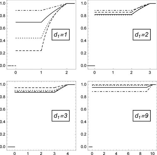
Therefore, the first-digit marginal of (8) becomes$$\begin{array}{c}{F}_{Z_{d_1}(X)}(z)=\left(1-\frac{{(d_1+1)}^{\alpha }-d_1^{\alpha }}{{10}^{\alpha }-1}\right){\mathrm{I}}_{[0,d_1[}(z)\\ +\left(1-\frac{{(d_1+1)}^{\alpha }-z^{\alpha }}{{10}^{\alpha }-1}\right){\mathrm{I}}_{[d_1,d_1+1[}(z)\\ +{\mathrm{I}}_{[d_1+1,\infty [}(z),\end{array}$$further specializing to (10) for α = 0. Figure 1 shows the shape of $F_{Z_{d_1}(X)}$ for selected values of α and d₁, when X follows the generalized Benford’s law. In each panel the (solid) line drawn for α = 0 yields the corresponding first-digit distribution function under Benford’s law, while that for α = 1 (dot-dashed line) corresponds to the Uniform distribution. The generalized Benford’s law does not display symmetry with respect to α, that is, negative parameter values yield structurally different patterns in $F_{Z_{d_1}(X)}$ than their positive counterparts: see, for example, the lines corresponding to $\alpha =-1$ and α = 1. However, note that X is distributed according to the generalized Benford’s law with parameter α if and only if $1/X$ is distributed according to the generalized Benford’s law with parameter $-\alpha$. We refer to Barabesi and Pratelli (2020) for further results on products of generalized Benford random variables. We prove in the Appendix that under the generalized Benford’s law(13) $$\mathrm{E}[Z_d(X)]=\{\begin{array}{cc}C\hfill & \alpha =0,\hfill \\ \frac{\alpha }{\alpha +1} \frac{{(c_d+1)}^{\alpha +1}-c_d^{\alpha +1}}{{10}^{k\alpha }-{10}^{(k-1)\alpha }}\hfill & \alpha \ne 0,\hfill \end{array}$$(13) which reduces to$$\mathrm{E}[Z_{d_1}(X)]=\{\begin{array}{cc}C\hfill & \alpha =0\hfill \\ \frac{\alpha }{\alpha +1} \frac{{(d_1+1)}^{\alpha +1}-d_1^{\alpha +1}}{{10}^{\alpha }-1}\hfill & \alpha \ne 0\hfill \end{array}$$ for k = 1. Again, the case α = 0 yields the sum-invariance property (5).

Fig. 1 Plot of $F_{Z_{d_1}(X)}$ for different values of $d_1\in \{1,\dots ,9\}$ and for $\alpha =-2$ (dashed line), $\alpha =-1$ (dotted line), α = 0 (solid line), and α = 1 (dot-dashed line), when X follows the generalized Benford’s law.

4 First-Digit Benford’s Law

We recall that, when the random variable X is Benford, characterization (2) is equivalent to both (3) and (5), while it implies (1) and (6). Instead, the first-digit properties (1) and (6) may still hold even if X is not Benford and condition (2) is not true. In such a case, we are interested in studying whether (1) is equivalent to (6), or (1) implies (6), or (1) is implied by (6). For simplicity, and with a slight abuse of notation, in what follows we take d = d₁ in such a way that $d\in \{1,\dots ,9\}$.

If X is an absolutely continuous random variable and S(X) admits a probability density function $f_{S(X)}$ with respect to the Lebesgue measure on $\mathbb{R}$, condition (1) is equivalent to(14) $${\pi }_d={\int }_d^{d+1}{f}_{S(X)}(t)dt={\hspace{0.17em}\text{log}\hspace{0.17em}}_{10}\left(\frac{d+1}{d}\right),$$(14) for all $d\in \{1,\dots ,9\}$, while condition (6) is equivalent to(15) $${\eta }_d={\int }_d^{d+1}t{f}_{S(X)}(t)dt=C,$$(15) for all $d\in \{1,\dots ,9\}$. Expressions (14) and (15) provide a system of functional equations in $f_{S(X)}$, with the constraint that $f_{S(X)}$ be a proper density function. It seems prohibitive to address the relationship between (1) and (6) in such a general setting, although inequalities involving π_d and η_d may be easily obtained. Indeed, by integrating ${\eta }_d={\int }_d^{d+1}t{f}_{S(X)}(t)dt$ by parts, it can be proved that$${\eta }_d=d{\pi }_d+F_{S(X)}(d+1)-{\int }_d^{d+1}{F}_{S(X)}(t)dt,$$ since ${\pi }_d=F_{S(X)}(d+1)-F_{S(X)}(d)$. By also recalling that $F_{S(X)}(d)\le {\int }_d^{d+1}{F}_{S(X)}(t)dt\le F_{S(X)}(d+1)$, the following two inequalities are then obtained:(16) $$d{\pi }_d\le {\eta }_d\le (d+1){\pi }_d$$(16)

and(17) $$\frac{{\eta }_d}{d+1}\le {\pi }_d\le \frac{{\eta }_d}{d}.$$(17)

To obtain workable results, it is convenient to consider for $f_{S(X)}$ the following family of simple functions(18) $$f_{S(X)}(t)=\sum _{d=1}^9(a_d{\mathrm{I}}_{[d,d+1/2[}(t)+b_d{\mathrm{I}}_{[d+1/2,d+1[}(t)),$$(18) where the coefficients a_d and b_d are real numbers that satisfy the set of constraints $a_d\ge 0,b_d\ge 0$ and ${\sum }_{d=1}^9(a_d+b_d)/2=1$. These constraints ensure that $f_{S(X)}$ is a bona fide probability density function. In such a case, we obtain(19) $${\pi }_d={\int }_d^{d+1}{f}_{S(X)}(t)dt=\frac{1}{2} a_d+\frac{1}{2} b_d,$$(19)

and(20) $${\eta }_d={\int }_d^{d+1}t{f}_{S(X)}(t)dt=\frac{4d+1}{8} a_d+\frac{4d+3}{8} b_d.$$(20)

The constants $({\pi }_1,\dots ,{\pi }_9)$ and $({\eta }_1,\dots ,{\eta }_9)$ must be chosen in such a way that they jointly satisfy the set of constraints on the coefficients $(a_1,\dots ,a_9)$ and $(b_1,\dots ,b_9)$. It follows from expressions (19) and (20) that(21) $$a_d=(4d+3){\pi }_d-4{\eta }_d$$(21) and(22) $$b_d=-(4d+1){\pi }_d+4{\eta }_d.$$(22)

If the set $({\pi }_1,\dots ,{\pi }_9)$ is fixed, from the nonnegativity of a_d and b_d, we thus obtain(23) $${\eta }_d\in \left[\left(d+\frac{1}{4}\right){\pi }_d,\left(d+\frac{3}{4}\right){\pi }_d\right],$$(23)

while if the set $({\eta }_1,\dots ,{\eta }_9)$ is fixed, it must hold(24) $${\pi }_d\in \left[\frac{{\eta }_d}{d+3/4},\frac{{\eta }_d}{d+1/4}\right],$$(24) with ${\sum }_{d=1}^9{\pi }_d=1$. It is worth noting that the previous bounds are close to the universal bounds obtained in (16) and (17). Therefore, the considered family of simple functions covers a wide range of models, also encompassing extreme situations.

We can see from (23) that the interval of values (if it exists) for which η_d is a fixed constant for $d=1,\dots ,9$, say ${\eta }_d=\eta$, is given by$$\eta \in \left[{\max }_d\left\{\left(d+\frac{1}{4}\right){\pi }_d\right\},{\min }_d\left\{\left(d+\frac{3}{4}\right){\pi }_d\right\}\right].$$

Therefore, if (1) holds, it can be easily shown that(25) $$\eta \in \left[\frac{37}{4}{\hspace{0.17em}\text{log}\hspace{0.17em}}_{10}\frac{10}{9},\frac{39}{4}{\hspace{0.17em}\text{log}\hspace{0.17em}}_{10}\frac{10}{9}\right].$$(25)

The interval given in (25) contains the value $\eta =C$, as it must be under Benford’s law.

We can retrieve the simple function $f_{S(X)}$ for which expressions (1) and (6) jointly hold, without necessarily assuming (2), by substituting the values ${\pi }_d={\hspace{0.17em}\text{log}\hspace{0.17em}}_{10}((d+1)/d)$ and ${\eta }_d=C$ in Equations (21)(21) $$a_d=(4d+3){\pi }_d-4{\eta }_d$$(21) and (22)(22) $$b_d=-(4d+1){\pi }_d+4{\eta }_d.$$(22) . The resulting function is displayed in Figure 2. In addition, on the basis of (25), we can obtain simple functions $f_{S(X)}$ such that (1) holds while ${\eta }_1=\dots ={\eta }_9=\eta$, but with $\eta \ne C$. These functions provide examples of cases where the first-digit marginal distribution (1) holds, albeit the corresponding sum-invariance property (6) does not. One similar instance is described in Section 6.1.

Fig. 2 The simple function $f_{S(X)}$ for which expressions (1) and (6) jointly hold.

Conversely, if ${\eta }_d=C$ for $d=1,\dots ,9$, we see from (24) that it must be(26) $${\pi }_d\in \left[\frac{C}{d+3/4},\frac{C}{d+1/4}\right],$$(26) with the constraint ${\sum }_{d=1}^9{\pi }_d=1$. Therefore, examples of simple functions $f_{S(X)}$ for which expression (6) is true, but expression (1) is not, can be easily achieved. We again refer to Section 6.1 for a similar instance. On the basis of the well-known inequalities on the Neper number, it is also worth noting that for the Benford’s first-digit probability (1) it holds$${\hspace{0.17em}\text{log}\hspace{0.17em}}_{10}\left(\frac{d+1}{d}\right)\in \left[\frac{C}{d+1},\frac{C}{d}\right],$$ in agreement with (17). Hence, the constraints provided by (26) are rather severe, as it can be numerically assessed. At least for the considered class of simple functions, when (6) holds the probabilities $({\pi }_1,\dots ,{\pi }_9)$ are likely to resemble rather closely to ${\hspace{0.17em}\text{log}\hspace{0.17em}}_{10}((d+1)/d)$, especially for $d\ge 3$.

5 A Battery of Sum-Invariance Test Statistics for the First Digit

5.1 Null Hypotheses and Significand-Based Test Statistics

Following the argument of Section 4, in the present section we detail the simple, but practically important, first-digit case. We again take d = d₁ in such a way that $d\in \{1,\dots ,9\}$.

Given a random sample $(X_1,\dots ,X_n)$ of n independent copies of X, the inferential target consists in assessing whether X is Benford. According to (2), this hypothesis is stated as$$H_0:S(X)\stackrel{\mathcal{L}}{=}{10}^U,$$or as $H_0:〈{\hspace{0.17em}\text{log}\hspace{0.17em}}_{10}\left|X\right|〉\stackrel{\mathcal{L}}{=}U$, where U is a Uniform random variable on $[0,1[$. However, a test of the strong Benford null H₀ might be considered too restrictive in practical applications owing to measurement limitations, since the realizations of X are often recorded up to few significant digits. We provide a more precise qualification of this common-sense statement in Section 6.1. As a consequence of the perceived limitations of H₀, the null hypothesis on the first digit$$H_0^{\text{digit}}:D_1(X)\stackrel{\mathcal{L}}{=}{D}_1({10}^U)$$ is often preferred by fraud examiners in practice. $H_0^{\text{digit}}$ does not imply H₀, but the converse is true. Rejection of $H_0^{\text{digit}}$ thus leads to rejection of H₀.

Similarly, in its simplest first-digit form, a sum-invariance test aims at assessing the one-dimensional null hypothesis(27) $$H_0^{\text{sum}}=\underset{d=1}{\overset{9}{\cap }}{H}_{0,d}^{\text{sum}},$$(27) where $H_{0,d}^{\text{sum}}:\mathrm{E}[Z_d(X)]=C$. According to property (6), the sub-hypotheses $H_{0,d}^{\text{sum}}$ must hold for all $d\in \{1,\dots ,9\}$ when X is Benford. As for $H_0^{\text{digit}}$, rejection of $H_0^{\text{sum}}$ leads to rejection of H₀. The connection between $H_0^{\text{sum}}$ and $H_0^{\text{digit}}$ originates from the relationship between the corresponding first-digit properties (6) and (1), investigated in Section 4. Furthermore, in Section 6, we show evidence that examination of the first-digit properties of X may, perhaps surprisingly, lead to more powerful conclusions about departure from Benford’s law than considering a test statistic specifically constructed for the assessment of H₀.

Several tests exist for $H_0^{\text{digit}}$. In what follows we define a battery of test statistics constructed for $H_0^{\text{sum}}$. To this aim, we consider the standardized sample mean$$T_d=\frac{{\overline{Z}}_d-C}{\sqrt{C(d+1/2-C)/n}},$$where$${\overline{Z}}_d=\frac{1}{n} \sum _{i=1}^n{Z}_d(X_i)$$ and the denominator is obtained from (11) with k = 1 and $d\in \{1,\dots ,9\}$. The developments in Section 4 show that the exact distribution function of the new test statistics under $H_0^{\text{sum}}$ will be tractable only in special cases. Their distribution is instead readily estimable under the more stringent Benford null H₀. Therefore, our suggestion in view of anti-fraud applications is to evaluate the significance of these statistics under H₀, even if they are defined under the more general $H_0^{\text{sum}}$, and to interpret them as proper tests of conformance to Benford’s law. We do the same with the available tests of $H_0^{\text{digit}}$. The consequences of this choice are assessed in Section 6.1, where we compare the behavior of the tests under the different hypotheses, and in Section 6.2 in terms of power under several alternatives when H₀ is the relevant null.

5.2 Hotelling-Type Test

Let $\overline{Z}={({\overline{Z}}_1,\dots ,{\overline{Z}}_9)}^{\mathrm{T}}$ and let μ be the vector of order 9 given by $\mu ={(C,\dots ,C)}^{\mathrm{T}}$. Under H₀, $\mathrm{E}[\overline{Z}]=\mu$ and$$\text{var}\left[\overline{Z}\right]=n^{-1}\Sigma ,$$where, according to (11) and (12), $\Sigma =({\sigma }_{dd\prime })$ is a $(9\times 9)$ matrix such that ${\sigma }_{dd}=C(d+1/2-C)$ and ${\sigma }_{dd\prime }=-C^2$ if $d\ne d\prime$. Hence, a Hotelling-type statistic is defined as$$Q=n{(\overline{Z}-\mu )}^{\mathrm{T}}{\Sigma }^{-1}(\overline{Z}-\mu ).$$

In principle, the distribution function of the test statistic Q under Benford’s law, say F_Q, could be computed exactly, but this task is prohibitive in practice. A Monte Carlo approximation of this distribution is instead readily available by bearing in mind that ${10}^U$ is a Benford random variable and that $S({10}^U)={10}^U$. Specifically, B Monte Carlo replicates of $\overline{Z}$, say ${\overline{Z}}_1^{\ast },\dots ,{\overline{Z}}_B^{\ast }$, are generated as$${\overline{Z}}_b^{\ast }={({\overline{Z}}_{1,b}^{\ast },\dots ,{\overline{Z}}_{9,b}^{\ast })}^{\mathrm{T}},$$where ${\overline{Z}}_{d,b}^{\ast }=n^{-1}{\sum }_{i=1}^n{Z}_d({10}^{U_{b,i}})$ and $(U_{b,1},\dots ,U_{b,n})$ are independent Uniform random variables on $[0,1[$, for $b=1,\dots ,B$. Therefore, B Monte Carlo replicates of Q, say $Q_1^{\ast },\dots ,Q_B^{\ast }$, are$$Q_b^{\ast }=n{({\overline{Z}}_b^{\ast }-\mu )}^{\mathrm{T}}{\Sigma }^{-1}({\overline{Z}}_b^{\ast }-\mu ),$$

yielding the Monte Carlo approximation of F_Q $$F_Q^{\ast }(q)=\frac{1}{B} \sum _{b=1}^B{\mathrm{I}}_{]-\infty ,q]}(Q_b^{\ast }).$$

Correspondingly, for a realization q of Q, the p-value $p_Q(q)=1-F_Q(q)$ is approximated by $p_Q^{\ast }(q)=1-F_Q^{\ast }(q)$. Finally, on the basis of Corollary 1.7 by Serfling (1980, p. 26), $Q\stackrel{\mathcal{L}}{\to }{\chi }_9^2$ as $n\to \infty$, where ${\chi }_{\nu }^2$ denotes the chi-square random variable with ν degrees of freedom.

5.3 Sup-Norm Test

A sup-norm test statistic for assessing $H_0^{\text{sum}}$ in (27) is(28) $$M={\max }_d\left|T_d\right|.$$(28)

This test rejects $H_0^{\text{sum}}$ for large realizations of M. Furthermore, if F_M denotes the distribution function of M under H₀ and $q_{M,1-\gamma /2}$ is its $(1-\gamma /2)$th quantile, simultaneous acceptance intervals at significance level γ for the marginal test statistics ${\overline{Z}}_1,\dots ,{\overline{Z}}_9$ are, for $d=1,\dots ,9$,(29) $$\begin{array}{c}[C-q_{M,1-\gamma /2}\sqrt{C(d+1/2-C)/n},\\ C+q_{M,1-\gamma /2}\sqrt{C(d+1/2-C)/n}].\end{array}$$(29)

These simultaneous acceptance intervals can supplement exploratory procedures, such as those presented by Nigrini (2012, chap. 5), with inferential statements about the digits involved in rejection of $H_0^{\text{sum}}$.

As shown in Section 5.2, Monte Carlo replicates of M can be generated as $M_b^{\ast }={\max }_d\left|T_{d,b}^{\ast }\right|$, for $b=1,\dots ,B$, where$$T_{d,b}^{\ast }=\frac{{\overline{Z}}_{d,b}^{\ast }-C}{\sqrt{C(d+1/2-C)/n}}.$$

From these replicates we obtain the Monte Carlo approximation of F_M, say $F_M^{\ast }(m)$, while $p_M^{\ast }(m)=1-F_M^{\ast }(m)$ is the approximated p-value for a realization m of M. Moreover,$$q_{M,1-\gamma /2}^{\ast }=\underset{u\in \mathbb{R}}{\inf }\left\{\frac{1}{B} \sum _{b=1}^B{\mathrm{I}}_{]-\infty ,u[}(M_b^{\ast })\ge 1-\gamma /2\right\}$$is the quantile estimate to be substituted for $q_{M,1-\gamma /2}$ in (29).

5.4 Min p-Value Test

Combination of p-values provides an alternative procedure for assessing the null hypothesis $H_0^{\text{sum}}$ and simultaneously the sub-hypotheses $H_{0,d}^{\text{sum}}$ (see, e.g., Rubin-Delanchy, Heard, and Lawson 2019, for a recent discussion in the field of anomaly detection in computer networks). If $F_{\left|T_d\right|}$ is the distribution function of $\left|T_d\right|$ under H₀, let $p_{\left|T_d\right|}(t_d)=1-F_{\left|T_d\right|}(t_d)$ be the p-value for a realization t_d of $\left|T_d\right|$. Moreover, let $\psi :{[0,1]}^9\to \mathbb{R}$ be a suitable combining function, usually chosen as a function of the minimum. The min-p-value test statistic is$$G=\psi (p_{\left|T_1\right|}(\left|T_1\right|),\dots ,p_{\left|T_9\right|}(\left|T_9\right|)).$$

If the test rejects $H_0^{\text{sum}}$ for large values of G, its p-value is $p_G(g)=1-F_G(g)$, where $g=\psi (p_{\left|T_1\right|}(t_1),\dots ,p_{\left|T_9\right|}(t_9))$ is a realization of G and F_G is the distribution function of G under H₀.

Now, $G_b^{\ast }=\psi (p_{\left|T_1\right|}^{\ast }(\left|T_{1,b}^{\ast }\right|),\dots ,p_{\left|T_9\right|}^{\ast }(\left|T_{9,b}^{\ast }\right|))$, for $b=1,\dots ,B$, provide B Monte Carlo replicates of G, where$$p_{\left|T_d\right|}^{\ast }(t_d)=\frac{1}{B} \sum _{b=1}^B{\mathrm{I}}_{]t_d,\infty [}(|T_{d,b}^{\ast }|).$$

The Monte Carlo approximation of F_G is then$$F_G^{\ast }(g)=\frac{1}{B} \sum _{b=1}^B{\mathrm{I}}_{]-\infty ,g]}(G_b^{\ast }),$$while $p_G^{\ast }(g^{\ast })=1-F_G^{\ast }(g^{\ast })$ is the Monte Carlo estimate of $p_G(g)$, with$$g^{\ast }=\psi (p_{\left|T_1\right|}^{\ast }(t_1),\dots ,p_{\left|T_9\right|}^{\ast }(t_9)).$$

The same $(U_{b,1},\dots ,U_{b,n})$ are now considered for computing $T_{1,b}^{\ast },\dots ,T_{9,b}^{\ast }$, to keep the dependence structure of $p_{\left|T_1\right|}(|T_{1,b}|),\dots ,p_{\left|T_9\right|}(|T_{9,b}|)$.

5.5 A Combined Test

Since $H_0^{\text{sum}}$ is not equivalent to $H_0^{\text{digit}}$, our final proposal is to consider a combined test statistic tailored to the null hypothesis $H_0^{\text{digit}}\cap H_0^{\text{sum}}$. The aim of this strategy is to develop a robust procedure with good power under different alternatives, such as those which are likely to be detected by focusing on $H_0^{\text{sum}}$ and $H_0^{\text{digit}}$ separately. For simplicity, we only detail the case where Q is combined with the first-digit Pearson’s statistic, that is,(30) $${\chi }^2=\sum _{d=1}^9\frac{{(N_d-n{p}_{D_1}(d))}^2}{n{p}_{D_1}(d)},$$(30)

with $N_d={\sum }_{i=1}^n{\mathrm{I}}_{\left\{d\right\}}(D_1(X_i))$. The choice of a suitable combining function $\varphi :{[0,1]}^2\to \mathbb{R}$ yields the test statistic$$L=\varphi (p_{{\chi }^2}({\chi }^2),p_Q(Q)),$$where, for a realization x of ${\chi }^2,p_{{\chi }^2}(x)=1-F_{{\chi }^2}(x)$ is the p-value and $F_{{\chi }^2}$ is the distribution function of ${\chi }^2$ under H₀. If the test rejects for large values of L, the p-value is $p_L(l)=1-F_L(l)$, where $l=\varphi (p_{{\chi }^2}(x),p_Q(q))$ is a realization of L and F_L is the distribution function of L under H₀.

As before, the Monte Carlo approximation of the distribution function of ${\chi }^2$ under H₀ is$$F_{{\chi }^2}^{\ast }(t)=\frac{1}{B} \sum _{b=1}^B{\mathrm{I}}_{]-\infty ,t]}({\chi }_b^{2\ast }),$$where the replicates ${\chi }_1^{2\ast },\dots ,{\chi }_B^{2\ast }$ of ${\chi }^2$ are generated as$${\chi }_b^{2\ast }=\sum _{d=1}^9\frac{{(N_{d,b}^{\ast }-n{p}_{D_1}(d))}^2}{n{p}_{D_1}(d)},$$ with $N_{d,b}^{\ast }={\sum }_{i=1}^n{\mathrm{I}}_{\left\{d\right\}}(\lfloor {10}^{U_{b,i}}\rfloor ))$ for $b=1,\dots ,B$. The p-value is approximated by $p_{{\chi }^2}^{\ast }(x)=1-F_{{\chi }^2}^{\ast }(x)$. Correspondingly, the B Monte Carlo replicates of L are $L_b^{\ast }=\varphi (p_{{\chi }^2}^{\ast }({\chi }_b^{2\ast }),p_Q^{\ast }(Q_b^{\ast }))$, for $b=1,\dots ,B$, where ${\chi }_b^{2\ast }$ and $Q_b^{\ast }$ are computed by means of the same $(U_{b,1},\dots ,U_{b,n})$. The Monte Carlo approximation of F_L is$$F_L^{\ast }(l)=\frac{1}{B} \sum _{b=1}^B{\mathrm{I}}_{]-\infty ,l]}(L_b^{\ast }),$$ while the Monte Carlo estimate of $p_L(l)$ is $p_L^{\ast }(l^{\ast })=1-F_L^{\ast }(l^{\ast })$, where $l^{\ast }=\varphi (p_{{\chi }^2}^{\ast }(x),p_Q^{\ast }(q))$.

5.6 Extension to the First-k Significant Digits

Generalization to the case k > 1 is straightforward, even if more cumbersome notation is required. We report the details as supplementary materials.

6 Simulation Study

As in Section 5, we consider sum-invariance test statistics based on the first-digit. We take the minimum as the combining function in the computation of L. For this test statistic, we write $L_{{\chi }^2,Q},L_{{\chi }^2,M}$, and $L_{{\chi }^2,G}$ when (30) is combined with Q, M, and G, respectively. In our simulation study, we address two major issues: the behavior of the tests when $H_0^{\text{digit}}$ and $H_0^{\text{sum}}$ hold, but H₀ does not, and their power under several alternative distributions, some of which are directly related to the anti-fraud context of our application domain. In the latter instance we take H₀ to be the relevant null, since the exact distribution function of the test statistics under $H_0^{\text{sum}}$ is not available in general, as emphasized in Section 4.

In anti-fraud operations related to international trade, like the one reported by European Commission (2014) and like those mentioned in Section 7, it is advisable to limit the number of false rejections, because substantial investigations are often demanding and time consuming. We thus display the results obtained when $\gamma =0.01$ is the nominal test size. A selection of results for $\gamma =0.05$ is instead given as supplementary materials. Unless otherwise stated, we take $B=1,000,000$ as the number of Monte Carlo replicates for estimating distribution functions. Rejection rates are computed on 100,000 independent simulation runs.

6.1 Test Behavior Under the First-Digit Benford’s Law

The Monte Carlo approximation to the distribution function of our test statistics assumes that the data are generated from a Benford random variable, implying that the samples are drawn from the strong Benford null hypothesis H₀. The resulting tests are thus exact under Benford’s law and their empirical size under the law will differ from the nominal one solely because of simulation error.

Since H₀ is more restrictive than $H_0^{\text{digit}}$ and $H_0^{\text{sum}}$, it is of interest to see the behavior of the tests when X satisfies one (or both) of these more general hypotheses but not H₀. We rely upon the results obtained in Section 4 to provide examples of this behavior. We elaborate the models belonging to class (18) in a variety of situations that span both worst-case scenarios and alternatives very close to H₀. Specifically, we consider the data generating models that follow:

1. Equations (21)(21) $$a_d=(4d+3){\pi }_d-4{\eta }_d$$(21) and (22)(22) $$b_d=-(4d+1){\pi }_d+4{\eta }_d.$$(22) with ${\pi }_d={\hspace{0.17em}\text{log}\hspace{0.17em}}_{10}((d+1)/d)$ and ${\eta }_d=C$ (see Figure 2), so that expressions (1) and (6) jointly hold, without necessarily assuming (2);

2. the lower endpoint of interval (23) with ${\pi }_d={\hspace{0.17em}\text{log}\hspace{0.17em}}_{10}((d+1)/d)$, so that $H_0^{\text{digit}}$ holds but $H_0^{\text{sum}}$ does not.

3. three instances where $H_0^{\text{sum}}$ holds but $H_0^{\text{digit}}$ does not, with ${\pi }_1,\dots ,{\pi }_9$ chosen to obtain:

   1. a “small” chi-square distance from Benford’s law within intervals (26), for $d=1,\dots ,9$; in the selected case the actual distance is 0.0002;

   2. an “intermediate” chi-square distance from Benford’s law within intervals (26), for $d=1,\dots ,9$; in the selected case the actual distance is 0.0014;

   3. the largest chi-square distance from Benford’s law within intervals (26), for $d=1,\dots ,9$; this distance is 0.0096.

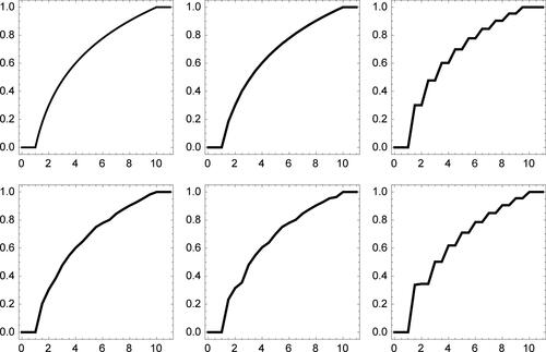
The distribution functions $F_{S(X)}$ associated to the five selected models are displayed in Figure 3, where they are also compared to the Benford’s distribution function (2). Case (a) is extremely close to H₀, as can be assessed both visually and numerically (the sup-norm distance from (2) is 0.008). Cases (b) and (c3) correspond instead to the most extreme deviations from H₀ in the considered class, the sup-norm distance of the distribution functions from (2) being 0.124 and 0.162, respectively. Alternatives (c1) and (c2) are milder and yield sup-norm distances from (2) of 0.026 and 0.058, respectively.

Fig. 3 Plot of $F_{S(X)}$ under different data-generating models. From left to right: Benford’s law, (a) and (b) (first row); (c1), (c2), and (c3) (second row). See text for explanation.

Table 1 gives the Monte Carlo estimate of the rejection probability for each test in the five instances described above and under the strong Benford null hypothesis H₀. The results refer to the case n = 100, while those for different sample sizes are reported as supplementary materials. In our comparison, we also include a Kolmogorov–Smirnov test statistic which is built upon characterization (2) of the significand function under Benford’s law. This statistic is defined as(31) $$\text{KS}=\underset{t\in [1,10[}{\sup }\left|{\widehat{F}}_{S(X)}(t)-{\hspace{0.17em}\text{log}\hspace{0.17em}}_{10}t\right|,$$(31) where ${\widehat{F}}_{S(X)}$ is the empirical distribution function of S(X) based on the available random sample $(X_1,\dots ,X_n)$. Strictly speaking, KS is constructed to provide a test of the strong Benford null H₀, not just of $H_0^{\text{sum}}$ and $H_0^{\text{digit}}$. It can thus be considered a sensible competitor to our tests when their focus is on checking the fit to Benford’s law, as it happens in the simulation study of Section 6.2 and in anti-fraud applications.

Table 1 Monte Carlo estimate of the rejection probability of each test under different data generating models, when n = 100.

Data generating model	${\chi }^2$	KS	Q	M	G	$L_{{\chi }^2,Q}$	$L_{{\chi }^2,M}$	$L_{{\chi }^2,G}$
Benford’s law: H0 true	0.010	0.009	0.010	0.010	0.010	0.010	0.010	0.010
(a): $H_0^{\text{digit}}$ and $H_0^{\text{sum}}$ true; H0 false	0.010	0.011	0.010	0.010	0.010	0.010	0.010	0.010
(b): $H_0^{\text{digit}}$ true; $H_0^{\text{sum}}$ false	0.010	0.303	1.000	0.004	0.006	1.000	0.008	0.008
(c1): $H_0^{\text{sum}}$ true; $H_0^{\text{digit}}$ false	0.010	0.012	0.010	0.010	0.010	0.010	0.009	0.010
(c2): $H_0^{\text{sum}}$ true; $H_0^{\text{digit}}$ false	0.010	0.034	0.011	0.010	0.011	0.011	0.011	0.011
(c3): $H_0^{\text{sum}}$ true; $H_0^{\text{digit}}$ false	0.015	0.604	0.018	0.012	0.013	0.019	0.016	0.016

NOTE: The nominal test size is 0.01.

The first two lines of Table 1 confirm that the joint set of constraints implied by the validity of both $H_0^{\text{digit}}$ and $H_0^{\text{sum}}$ (model (a)) makes the distribution of each test statistic virtually indistinguishable from that obtained under the strong Benford null H₀. In this case even the omnibus KS test is not able to detect the departure from H₀ with customary sample sizes and much larger values of n are required. For instance, the power of KS under model (a), computed for simplicity over 1000 replications, raises to 0.052 if $n=10,000$.

When moving to the scenario where only $H_0^{\text{sum}}$ is true (models (c1)–(c3)), we first note that class (18) provides a rather extreme choice with respect to H₀, since it gives rise to absolutely continuous distribution functions for S(X) which are not differentiable at 18 points. We also recall that the universal bounds for π_d under $H_0^{\text{sum}}$, given in (16), are fairly close to those obtained from (26). The considered class is thus convenient to assess the behavior of our sum-invariance tests in a relatively unfavorable framework. By imposing more realistic models (e.g., by considering continuously differentiable distribution functions for S(X)), the proposed tests should arguably improve their empirical performance under $H_0^{\text{sum}}$ when significance is instead evaluated under the more stringent H₀.

In spite of the “pessimistic” nature of the selected class, the empirical size of our tests is close to the nominal value under both models (c1) and (c2). In the supplementary materials, it can be seen that the same conclusion is also true when $\gamma =0.05$ and when n = 500. Therefore, the distribution functions of our test statistics under H₀ are good approximations to those under $H_0^{\text{sum}}$ for customary sample sizes even when the two hypotheses are relatively far apart. On the other hand, assuming H₀ when model (c2) holds can have more severe consequences on the Kolmogorov–Smirnov test, especially when n is of the order of a few hundreds (see the supplementary materials). This result reinforces the idea that a test specifically tailored to H₀, such as KS, may be too stringent under moderate violations of Benford’s law which are very unlikely to correspond to frauds, since $H_0^{\text{sum}}$ is still satisfied.

The least favorable choice for our tests under $H_0^{\text{sum}}$ is data generating model (c3), where the true density $f_{S(X)}$ is the farthest admissible one from Benford’s law within class (18). Even in this problematic instance the empirical size of M and G is close to the nominal target. Both Q and ${\chi }^2$ instead exhibit some liberality, thus showing moderate discrepancy between the actual test distribution and the approximation provided by the Monte Carlo procedure described in Section 5. Although the performance of our approach is not ideal in this scenario, we note that similar and even worse degrees of liberality may hold for the asymptotic version of the chi-square test (see, e.g., Cerioli et al. 2019, Table 1), which is often the selected choice in practice. Furthermore, a correction procedure similar to that proposed in Cerioli et al. (2019), and applied in Section 7.2, can be adopted if strict control of the nominal size under $H_0^{\text{sum}}$ is deemed necessary. This procedure, which can be easily extended should class (18) be replaced by a wider family of density functions, computes the Monte Carlo estimates of the null quantiles under model (c3) and compares the observed test statistics to such quantiles. The sum-invariance tests thus become exact under the least favorable specification of $H_0^{\text{sum}}$. They also become slightly conservative under the other models that satisfy $H_0^{\text{sum}}$ and that are closer to H₀. To provide a quantification of the corresponding conservativeness, in the supplementary materials we repeat the information given in Table 1 when the null distribution function of each test statistic is estimated by Monte Carlo simulation from model (c3).

The situation is considerably different when only $H_0^{\text{digit}}$ holds. The distribution of ${\chi }^2$ is virtually unchanged by this relaxation of the data-generating process, even if model (b) is the most extreme choice in the selected class. The effect on both KS and Q is instead paramount. It is perhaps surprising to see that the rejection rate of the first-digit statistic Q is much higher than that of the significand-based statistic KS, which is specifically constructed to provide a test of the strong Benford null H₀. However, we argue that this is a positive feature of Q in view of anti-fraud applications, since it is much easier in practice to fabricate first digits that conform to (1) than to replicate the sum-invariance property (6). One reason for the large power of Q under model (b) is that the generalized variance of $\overline{Z}$ is much smaller than under Benford’s law. The deviance matrix $n\text{var}[\overline{Z}]$ under model (b), say $\Upsilon$, is reported in the supplementary materials and we obtain$$\det (\Upsilon \mathrm{ }{\Sigma }^{-1})=0.11.$$

The information provided by the random vector $\overline{Z}$ and by its full covariance matrix can thus outperform a complete test of fit of model (2) if just the first-digit distribution conforms to Benford’s law. Further examples of the advantages of Q in possibly fraudulent situations where $H_0^{\text{digit}}$ holds, but H₀ does not, are reported in the sections below.

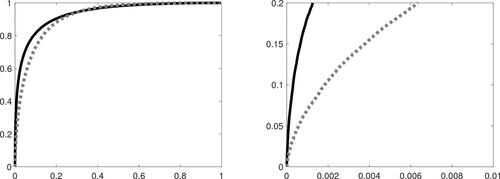
We conclude our analysis of model (b) by noting the remarkable difference in power between the Hotelling-type and the other two sum-invariance tests. The reason is the peculiar distribution of M and G, which turns out to be more concentrated than under Benford’s law. Figure 4 compares the estimated quantiles of M under the two models, in the case n = 100. The shorter right tail of the distribution of M under model (b) yields a reduced variability of the test statistic, whose standard error drops from 0.55 under H₀ to 0.49 under model (b). A corresponding decrease is observed for the 99th quantile. Such a peculiar behavior can be explained by looking at Table 2, which reports the estimates of $\mathrm{E}(|T_d|)$ and $\text{var}(|T_d|)$, for $d=1,\dots ,9$, under both models. When H₀ holds all the first-digit statistics have roughly the same mean and the same variance, thus ensuring good properties to the sup-norm metric in (28). On the contrary, we observe a noticeable shift in the parameters of $\left|T_1\right|$ under model (b). The resulting heteroscedasticy is not taken into account by M, as it instead happens with Q.

Fig. 4 Quantile plot comparing the empirical distribution of M when X is a Benford random variable (horizontal axis) with the same distribution when X is generated according to model (b) (vertical axis), in the case n = 100. Both distributions are estimated from 100,000 Monte Carlo replicates.

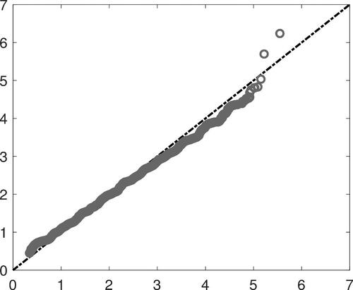
Table 2 Monte Carlo estimates of $\mathrm{E}(|T_d|)$ and $\text{var}(|T_d|)$, for $d=1,\dots ,9$, under H₀ (Benford’s law) and model (b), based on 100,000 Monte Carlo replicates.

		d = 1	d = 2	d = 3	d = 4	d = 5	d = 6	d = 7	d = 8	d = 9
H0	$\mathrm{E}(|T_d|)$	0.794	0.798	0.799	0.803	0.794	0.801	0.797	0.793	0.805
	$\text{var}(|T_d|)$	0.359	0.362	0.361	0.363	0.370	0.360	0.363	0.372	0.350
Model (b)	$\mathrm{E}(|T_d|)$	1.002	0.802	0.781	0.774	0.774	0.767	0.769	0.785	0.788
	$\text{var}(|T_d|)$	0.453	0.342	0.326	0.325	0.327	0.339	0.349	0.338	0.336

6.2 Power Comparison

We now investigate the ability of our tests, as well as that of ${\chi }^2$ and KS, to detect departures from Benford’s law in a number of practically relevant alternative models, some of which can be directly related to the anti-fraud context of our application domain. The null distribution function of each test statistic is estimated using the Monte Carlo procedure described in Section 5. Therefore, all the tests under comparison are exact under H₀ and their empirical performance under the strong Benford null is shown in the first line of Table 1.

In our first power scenario we assume that X is a Lognormal random variable, so that the observed data come from one of the most frequently adopted distributional models in many fields, including the analysis of the economic aggregates that arise in international trade (Barabesi et al. 2016a, 2016b). It is well known (Berger and Hill 2015, p. 55) that a Lognormal random variable becomes practically indistinguishable from a Benford random variable when the shape parameter is large. Therefore, this popular data-generating mechanism provides an alternative to Benford’s law whose separation from the null model can be continuously indexed by its shape parameter. We take the scale parameter equal to 1, but similar results have been observed for different choices. In our simulations, the shape parameter ranges between 0.5 and 0.8, since outside this interval all the tests share similar performances. Table 3 shows the power of our tests, together with that of the Pearson’s chi-square statistic (30) and of the Kolmogorov–Smirnov statistic (31), when n = 100. The results for different sample sizes are reported as supplementary materials. All our tests have sensible properties, with power converging to 1 as the shape parameter of the Lognormal distribution decreases and as the sample size grows (see the supplementary materials). There is a considerable advantage of Q over M and G, due to the information provided by the deviance matrix $n\text{var}[\overline{Z}]$.

Table 3 Estimated power when X is a Lognormal random variable with scale parameter 1, for different values of the shape parameter and n = 100.

Shape parameter	${\chi }^2$	KS	Q	M	G	$L_{{\chi }^2,Q}$	$L_{{\chi }^2,M}$	$L_{{\chi }^2,G}$
0.5	0.952	0.733	0.961	0.432	0.484	0.961	0.933	0.932
0.6	0.454	0.254	0.472	0.140	0.140	0.473	0.394	0.393
0.7	0.111	0.073	0.115	0.051	0.047	0.114	0.091	0.091
0.8	0.032	0.027	0.033	0.024	0.020	0.033	0.029	0.028

NOTE: The nominal test size is 0.01.

Since no parameter is estimated under Benford’s law, taking into account the full covariance matrix of $\overline{Z}$ does not lead to overfitting and can thus be recommended.

Our Hotelling-type test also shows a considerable advantage over the KS test of H₀ provided by (31), and a slight but systematic improvement over the chi-square test derived under $H_0^{\text{digit}}$. The advantage of Q over KS is further documented in Figure 5, which contrasts the empirical distribution of the p-values computed from each test statistic under the Lognormal model with shape parameter 0.6 (horizontal axis) to the Uniform distribution of the same p-values under H₀ (vertical axis). It is clearly seen that the distribution of Q under this alternative is considerably farther from the null than that of KS, and especially so in the right tail, where a much larger proportion of very small p-values is observed.

Fig. 5 Left-hand panel: Quantile plot comparing the empirical distribution of the p-values computed from Q (solid line) and from KS (dashed line) when X is a Lognormal random variable with shape parameter 0.6 (horizontal axis) with the Uniform distribution (vertical axis), in the case n = 100. Right-hand panel: Zoom of the quantile plot in a rectangular area close to the origin.

Our second power scenario assumes that X comes from another popular distributional model in economic and engineering applications. Specifically, we take X to be distributed according to a Weibull distribution whose shape parameter ranges between 1.2 and 2.2. Also in this case departure from Benford’s law can be indexed by the shape parameter, since a Weibull random variable is reasonably close to be Benford when the shape parameter is not too large (Miller 2015, §3.5.3). Explicit error estimates for convergence of Weibull distributions to Benford’s law can be found in Dümbgen and Leuenberger (2008, 2015), while Engel and Leuenberger (2003), Miller and Nigrini (2008), and Berger and Twelves (2018) addressed the special case of the Exponential distribution. We take the scale parameter equal to 1, but similar results have been observed for different choices. Table 4 gives the findings when n = 100, while those for different sample sizes are reported as supplementary materials. Our results confirm those obtained under the Lognormal alternative, with Q considerably more powerful than M, G and also KS, except when X comes very close to be Benford. We thus see that first-digit test statistics still outperform the ideally more stringent test based on (31) for a large part of the parameter space where comparison among tests is useful. These results also suggest that for the Weibull distribution there might be more effective discrepancy measures than the Kolmogorov–Smirnov metric considered by Miller (2015, p. 101), at least in this part of the parameter space.

Table 4 Estimated power when X is a Weibull random variable with scale parameter 1, for different values of the shape parameter and n = 100.

Shape parameter	${\chi }^2$	KS	Q	M	G	$L_{{\chi }^2,Q}$	$L_{{\chi }^2,M}$	$L_{{\chi }^2,G}$
1.2	0.037	0.048	0.038	0.025	0.026	0.038	0.032	0.034
1.4	0.113	0.087	0.116	0.050	0.131	0.116	0.093	0.095
1.6	0.289	0.170	0.302	0.096	0.097	0.303	0.242	0.242
1.8	0.554	0.327	0.583	0.192	0.205	0.583	0.492	0.493
2.0	0.799	0.546	0.834	0.367	0.402	0.833	0.751	0.754
2.2	0.936	0.764	0.958	0.588	0.630	0.957	0.913	0.916

NOTE: The nominal test size is 0.01.

In our third power scenario, we model the digit distribution directly and we take X to be distributed according to the generalized Benford’s law with $\alpha \ne 0$. For instance, under this model the first-digit masses span from $p_{D_1}(1)=0.556$ to $p_{D_1}(9)=0.012$ when $\alpha =-1$, while we recover the uniform first-digit distribution $p_{D_1}(1)=\cdots =p_{D_1}(9)=1/9$ when α = 1. Table 5 reports power for selected values of $\alpha \in [-0.8,0.8]$ when n = 100, while we again refer to the supplementary materials for further sample sizes. The generalized Benford distribution appears to be the least favorable case for first-digit test statistics because KS is the most powerful choice for all values of α. Furthermore, there is no systematic winner between Q and ${\chi }^2$, since the former dominates when $\alpha <0$ and the latter is to be preferred for $\alpha >0$. However, the performance of the simple combiner $L_{{\chi }^2,Q}$ is consistently close to the best solution provided by either Q or ${\chi }^2$. We thus conclude that combination of these two test statistics provides a robust strategy when the direction of the departure from Benford’s law is unknown. A further strategy, suggested by the results in Table 5, will be to combine Q and KS, to borrow strength from the best performer under the specific alternative. We will pursue this path in future research.

Table 5 Estimated power under the generalized Benford’s law with parameter $\alpha \ne 0$, for n = 100.

α	${\chi }^2$	KS	Q	M	G	$L_{{\chi }^2,Q}$	$L_{{\chi }^2,M}$	$L_{{\chi }^2,G}$
–0.8	0.839	0.989	0.860	0.687	0.758	0.861	0.814	0.830
– 0.6	0.445	0.869	0.475	0.337	0.417	0.474	0.421	0.457
–0.4	0.106	0.469	0.121	0.086	0.122	0.119	0.103	0.125
0.4	0.254	0.379	0.238	0.133	0.132	0.244	0.223	0.224
0.6	0.652	0.809	0.631	0.371	0.389	0.641	0.607	0.612
0.8	0.932	0.980	0.925	0.697	0.722	0.929	0.914	0.916

NOTE: The nominal test size is 0.01.

Our last power scenario refers to a potentially relevant instance of fraud. Therefore, it is directly related to the application domain considered in Section 7. In this scenario we mimic the behavior of a probability-savvy fraudster who ensures compliance of the first few digits of X to Benford’s law, but is not able to ensure that X is truly Benford, due to administrative or accounting constraints. For instance, Nigrini (2012, p. 255) reports the possibly suspect case of the list of payments made shortly before bankruptcy by a major company. This list shows almost perfect compliance with the two-digit extension of (1), thus calling for the use of more complex analytical tools than digit-conformance tests. Similar cautionary claims about the validity of (1) in the presence of data manipulation abound in the digital forensic literature (see, e.g., Kossovsky 2015, p. 82), while some studies seem to indicate that people need not be terribly bad at inventing numbers (Nigrini 2012, chap. 13), even without the help of random simulation. An example of this subtle, but potentially very dangerous, contamination framework is given in Table 6, where $D_1(X)$ follows (1) while the other digits of X are generated according to the generalized Benford’s law with parameter α. We display the results for n = 200 and n = 500, but similar patterns are observed with smaller sample sizes. As expected, the first-digit Pearson’s statistic (30) is not able to detect the departure from Benford’s law. Therefore, as a benchmark we now compute the two-digit version of (30), ${\chi }^{2\left\{2\right\}}$ in the notation of the supplementary materials, which is sometimes advocated as the primary choice in applications with moderate sample sizes (see, e.g., Nigrini 2012, p. 78). It is clearly seen that Q often outperforms ${\chi }^{2\left\{2\right\}}$ to a large extent, even if use of the latter implicitly assumes the additional (but usually unknown) information that contamination occurs in one of the first-two digits and not in the subsequent ones. The power values (not shown in the table) of M and G are instead inferior in this example, as they are under model (b) in Table 1. We thus argue that also in this framework information on the covariance structure of $\overline{Z}$ is essential to detect departure from Benford’s law when some of the digits marginally do follow the law. Surprisingly, the performance of KS is extremely poor in this setting, in spite of the fact that all the digits after the first one follow a generalized Benford’s model, against which test (31) was seen to have the largest power.

Table 6 Estimated power when $D_1(X)$ follows (1) while the other digits of X follow the generalized Benford’s law with parameter α.

	n = 200				n = 500
α	${\chi }^2$	${\chi }^{2\left\{2\right\}}$	KS	Q	${\chi }^2$	${\chi }^{2\left\{2\right\}}$	KS	Q
–1	0.010	0.034	0.016	0.054	0.010	0.155	0.022	0.226
– 0.6	0.010	0.016	0.012	0.015	0.010	0.036	0.014	0.028
0.6	0.010	0.016	0.010	0.036	0.011	0.026	0.013	0.107
1	0.010	0.020	0.010	0.065	0.010	0.046	0.016	0.239
2	0.010	0.034	0.011	0.151	0.010	0.117	0.028	0.564
3	0.010	0.047	0.013	0.241	0.010	0.212	0.042	0.770

NOTE: The nominal test size is 0.01.

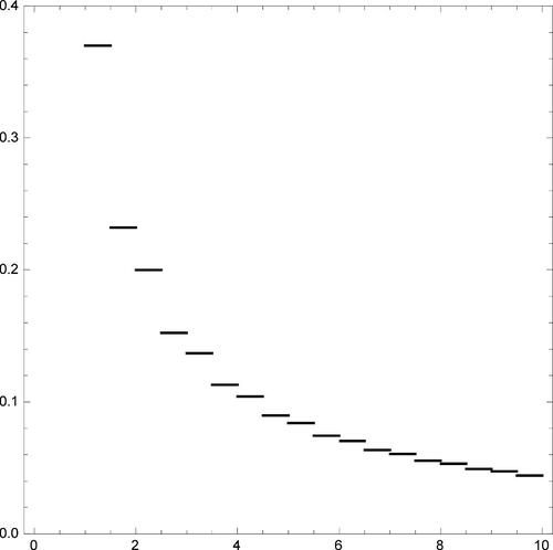
Finally, we show that our sum-invariance statistics are not affected by contamination in the last significant digits, like rounding errors or other numerical inaccuracies, although all the recoded digits of X are involved in their computation through the standardized sample means $T_1,\dots ,T_9$. In particular, we report the results obtained when each Benford random variable in the sample, simulated according to (2), is multiplied by ${10}^K$. The order of magnitude K is randomly sampled from an empirical data base of customs declarations with the constraint that $K>K_{\min }$ and $K_{\min }\in \{2,3,4,5\}$. The first three digits are then retained, while the others are set equal to zero. Table 7, drawn for the different values of $K_{\min }$, shows that the power under this contamination scheme is virtually indistinguishable from the test size, meaning that the number of rejections induced by the truncated digits is negligible. This is another important property of test statistics for their use in anti-fraud applications, since rounding and inaccuracies in data typically have very different implications than data fabrication (see, e.g., Diaconis and Freedman 1979).

Table 7 Estimated power of sum-invariance statistics under truncation to 0 of the last digits of a Benford random variable (see the text for details), with n = 200.

$K_{\min }$	Q	M	G
2	0.0102	0.0097	0.0096
3	0.0100	0.0100	0.0097
4	0.0098	0.0093	0.0093
5	0.0102	0.0096	0.0096

NOTE: The nominal test size is 0.01.

7 Application to the Detection of Customs Frauds

7.1 Analysis of Trade Data

To show the potential of our sum-invariance tests for the purpose of fraud detection, we describe their application to the transaction data reported in the customs declarations of two traders for which one instance of fraudulent underreporting of the declared value, a so-called undervaluation, was found. These data were collected in the context of a specific operation on import undervaluation in a member state of the European Union. Such anti-fraud operations typically rely on sophisticated risk profiling systems that aim at predicting possible frauds on the basis of the combination of various types of alerts. These systems often give large weight to the signals provided by outlier detection tools that are applied to monthly-aggregated data (see Perrotta et al. 2020, and the references therein), thus not being directly comparable to the present proposal. Furthermore, an important issue in the identification of customs frauds by means of outlier diagnostics is that substantive controls are costly and time consuming, so that only a very limited number of individual transactions are usually checked for each suspected trader. It is then essential that statistical tests provide a hint to the cases where more controls are needed. Our sum-invariance approach is a natural candidate to fulfill this need, since it is particularly effective for the purpose of hunting serial fraudsters (see Section 7.2).

For the first trader that we analyze n = 171, but only 6 transactions were actually checked. The p-value of the Pearson’s statistic (30) is 0.023, suggesting only mild evidence of data manipulation in the whole set of transactions. On the contrary, for the sum-invariance tests we obtain q = 25.326, m = 3.402, and g = 0.999, yielding p-values $p_Q^{\ast }(q)=0.003,p_M^{\ast }(m)=0.009$ and $p_G^{\ast }(g)=0.007$, respectively. Combination of ${\chi }^2$ and Q retains the high power of the sum-invariance test, since $p_L^{\ast }(l^{\ast })=0.004$. Therefore, our approach suggests that more transactions of this trader should be checked in the search for frauds.

For the second trader we observe n = 292 transactions, of which only 3 were checked. The results that we obtain resemble those for the savvy contamination scheme described in Section 6.2, since the p-value of (30) is 0.611, whereas $p_Q^{\ast }(q)=0.005,p_M^{\ast }(m)=0.555$, and $p_G^{\ast }(g)=0.559$. Therefore, Q points to the conclusion that more transactions could have been manipulated, even if their first-digit distribution conforms to Benford’s law. Combination of ${\chi }^2$ and Q again provides a powerful, yet robust, strategy, yielding a p-value of 0.006. In this example the information mainly comes from the inclusion in the test statistic of the null covariance structure of the standardized averages $({\overline{Z}}_1,\dots ,{\overline{Z}}_9)$ involving all the recorded digits. Further inspection of the trader indeed shows strong discrepancy between the estimated conditional probabilities of subsequent digits given the first one and the corresponding values expected under Benford’s law (see Hill 1995b, p. 355). For instance, for $d_2\in \{0,1,\dots ,9\}$, Table 8 reports the estimates of $P(D_2(X)=d_2|D_1(X)=1)$ computed for this trader, together with the null conditional probabilities obtained from (4). The chi-square statistic for this table (based on a subset of 91 transactions) is 23.12 and suggests strong disagreement between estimated and null conditional digit probabilities. Neither (30) nor its multi-digit extensions would be able to detect this subtle departure from Benford’s law, whose anti-fraud implications are worth to be investigated.

Table 8 Estimates of the conditional probabilities $P(D_2(X)=d_2|D_1(X)=1)$ for $d_2\in \{0,1,\dots ,9\}$ (first row), and their values under Benford’s law (second row).

$d_2=0$	$d_2=1$	$d_2=2$	$d_2=3$	$d_2=4$	$d_2=5$	$d_2=6$	$d_2=7$	$d_2=8$	$d_2=9$
0.077	0.055	0.132	0.055	0.066	0.143	0.132	0.088	0.165	0.088
0.138	0.126	0.115	0.107	0.100	0.093	0.087	0.082	0.078	0.074

7.2 Comparison With Outlier Detection

Following Bolton and Hand (2002), most unsupervised fraud detection methods look for anomalies in the data. Therefore, all of these techniques assume (either explicitly or implicitly) that the available data have been generated by a k-variate random vector, say Y, whose distribution function F_Y is an (unknown) element within the following family $\mathcal{C}$ of distribution functions (see, e.g., Cerioli, Farcomeni, and Riani 2019, and the references therein)(32) $$\mathcal{C}=\{F_Y:F_Y=(1-\lambda )F_0+\lambda F_1,\lambda \in [0,1\left[\right\}.$$(32)

In this model, F₀ is the distribution function of the “good” part of the data, that is, F₀ represents the postulated null model, F₁ is the contaminant distribution, which is usually left unspecified except at most for the assumption of some regularity conditions, and λ is the contamination rate. Consistent estimation of the parameters in F₀, which is crucial for correct identification of the outliers, requires the adoption of robust high-breakdown techniques and often assumes Y to be normally distributed in the absence of contamination. See, for example, Cerioli (2010), Riani, Atkinson, and Perrotta (2014), Riani, Corbellini, and Atkinson (2018), and Rousseeuw et al. (2019) for a description of relevant methods in the anti-fraud domain.

Cast in the framework of international trade, where k = 1 and the value of an individual import transaction originates from the product of the traded amount with the unit price, a simple form of the postulated null model in (32) is(33) $$F_0(y)=\Phi \left(\frac{y-{\beta }_0-{\beta }_{1}v}{b}\right),$$(33) where y denotes the transaction value and v is the traded amount, both on a logarithmic scale, β₀ and β₁ are unknown parameters, and $\Phi$ is the distribution function of a standard Normal random variable. Therefore, if a random sample of N transaction values is available together with the associated traded amounts, yielding vectors $(Y_1,\dots ,Y_N)$ and $(v_1,\dots ,v_N)$, it is assumed that in the absence of fraud each transaction follows the simple regression model(34) $$Y_i={\beta }_0+{\beta }_1{v}_i+{ϵ}_i,$$(34) for $i=1,\dots ,N$, where ${ϵ}_1,\dots ,{ϵ}_N$ are independent Normal errors with mean 0 and variance b². In this setting, λ defines the probability of contamination, and thus of potential fraud, for each transaction drawn from population (32). Therefore, for transaction i we have that $\lambda ={\lambda }_i$ and outlier detection aims at checking whether ${\lambda }_i=0$, for $i=1,\dots ,N$.

Our conformance tests to Benford’s law instead rely on a different specification of contamination model (32) for international trade data. Although k = 1 as in (33), in our framework Y is the significand of the transaction value and(35) $$F_0(t)={\hspace{0.17em}\text{log}\hspace{0.17em}}_{10}t {\mathrm{I}}_{[1,10[}(t)+{\mathrm{I}}_{[10,\infty [}(t),$$(35) as in (2). It is apparent that no parameter has to be estimated under model (35). Even more importantly, our operational generating model for outlier-free significands is trader-specific. Given a set of L traders, the model for trader l is written as(36) $$Y_{i,l}={10}^{U_i},$$(36) where $i=1,\dots ,n_l$ and $l=1,\dots ,L,Y_{i,l}$ is the significand of the ith transaction value for trader l, n_l is the total number of transactions for this trader and U_i is a Uniform random variable on $[0,1[$. Cerioli et al. (2019) investigated the trade conditions under which (36) may yield a reasonable approximation for the first-digit distribution of the customs values of the selected trader. They also suggested a correction to the distribution of Pearson’s statistic (30) when these conditions are not met. Since λ now defines the probability of contamination among the transactions of trader l, that is, $\lambda ={\lambda }_l$, rejection of the hypothesis ${\lambda }_l=0$ labels trader l as a potential fraudster. This information is not available under model (33).

Comparison of models (34) and (36) shows that outlier detection and conformance to Benford’s law look at different types of anomalies. They also entail different computational efforts, since the former requires that a complex algorithm for robust parameter estimation be applied to a potentially very large number N of market transactions, while the latter only needs L repeated calls to a goodness-of-fit algorithm which is generally fast (even allowing for Monte Carlo estimation of the test distribution).

It may be expected that outlier detection could help to identify large individual frauds in specific markets, while Benford analysis could be beneficial for the labeling of serial fraudsters. To provide empirical evidence of this intuition, in what follows we make the simplifying assumption that only one product originates all the transactions under investigation, so that (34) may become a suitable data generating model for outlier-free data, on a logarithmic scale. Among the five robust regression methods applied to trade data by Riani, Atkinson, and Perrotta (2014), we first adopt least trimmed squares (LTS) to estimate the parameters in (34) and to identify the outliers. We perform our analysis with the implementation of LTS which is available in the MATLAB FSDA toolbox described by Perrotta et al. (2020, p. 9) and accessible from http://rosa.unipr.it/fsda.html. This algorithm appears to be reasonably fast with just one predictor, allowing us to handle a realistic number of traders and market transactions. We select the default initialization option, involving examination of 3000 random subsamples, and a breakdown value of 0.25. The latter is often deemed to be a sensible compromise between robustness and efficiency when the expected number of outliers in not too large (Hubert, Rousseeuw, and Van Aelst 2008, p. 95). Outlier labeling comes from the analysis of robust regression residuals, which can be compared to their asymptotic Normal distribution when the number of transactions is large. We set 0.01 as the nominal test size for outlier detection, to ensure comparison with the simulation results in Section 6.2. Correspondingly, we apply the correction method of Cerioli et al. (2019) to the distribution of our sum-invariance tests, as well as to the distribution of ${\chi }^2$ and KS, since (35) is not an adequate model under a trade scenario involving just one product. The nominal size of such tests is again 0.01.

We simulate transaction values for L = 1000 “idealized” traders of the selected product, whose specific description is omitted for confidentiality reasons. This product is chosen, after appropriate anonymization that makes it impossible to infer the features of individual operators, from a national database of one calendar-year customs declarations (see Cerioli et al. 2019, for further details on the data). Our simulation scheme is able to mimic the main features observed in the original market of the product. Therefore, in the selection process we have carefully avoided the products involving multiple populations, a pattern that often affects customs trade data (Cerioli and Perrotta 2014; Cerasa, Torti, and Perrotta 2016) but that violates the assumption of model (34) for genuine transactions. We assume that each idealized operator trades a constant number of n_l = 100 transactions, thus replicating the case n = 100 described in Section 6.2. The total number of transactions for outlier detection in (34) is then $N=100,000$, with the assumption that at least $N/4+1$ of them follow the null model. For simplicity, in our trader-specific version of contamination model (32) we also assume that each fraudster has the same propensity to fraud, so that λ_l is constant among the cheating traders. It is worth noting that the absence of parameters to be estimated under (35) allows us to extend model (32) to include the extreme case ${\lambda }_l=1$, defining a “complete” fraudster.

We generate noncontaminated transactions by picking unit price and traded quantity of the selected product at random from the same national database of customs declarations. Specifically, we adopt a product-constrained version of the simulation algorithm of Cerioli et al. (2019, SI Appendix, §2) and we randomly assign each transaction to a trader. The first column of Table 9 reports the empirical size of the Benford tests Q, X², and KS (for these tests size corresponds to the instance where ${\lambda }_l=0$ for $l=1,\dots ,L$) and also the empirical size of outlier detection through LTS, over 100 replications of the market simulation exercise. It is seen that all the Benford methods provide good control of the proportion of false fraud signals when indeed no contamination is present in the data, while LTS turns out to be somewhat conservative with this kind of data structures. They also confirm that the correction method of Cerioli et al. (2019) works equally well for Q and KS, as it was for ${\chi }^2$.

Table 9 Estimated size and power over 100 replications of the market simulation exercise for different proportions τ of fraudsters (the corresponding propensity to fraud of each fraudster l, λ_l, is also shown).

	Size	$\tau =0.4$	$\tau =0.2$	$\tau =0.1$	$\tau =0.08$	$\tau =0.05$	$\tau =0.04$
	${\lambda }_l=0$	${\lambda }_l=0.1$	${\lambda }_l=0.2$	${\lambda }_l=0.4$	${\lambda }_l=0.5$	${\lambda }_l=0.8$	${\lambda }_l=1$
Q	0.009	0.025	0.102	0.777	0.983	1.000	1.000
X^2	0.010	0.026	0.070	0.318	0.517	0.959	1.000
KS	0.010	0.036	0.138	0.694	0.911	1.000	1.000
LTS	0.002	0.393	0.392	0.392	0.391	0.392	0.391

NOTE: The nominal size of each test is 0.01. The contamination scheme is described in the supplementary materials.

We then contaminate 4000 transactions in the market through the digit contamination scheme which is detailed in the supplementary materials. The artificially introduced frauds are uniformly split within a proportion τ of fraudulent traders, with $\tau \in \{0.04,0.05,0.08,0.1,0.2,0.4\}$. This framework allows us to compare our Benford analysis with outlier detection under different cheating scenarios. For instance, if $\tau =0.04$ we only have 40 fraudsters among the 1000 traders and all the 100 transactions of each fraudster are then contaminated, yielding ${\lambda }_l=1$ if trader l is a fraudster and ${\lambda }_l=0$ otherwise. On the opposite end, if $\tau =0.4$ as many as 400 traders are cheating, but all of them in 10 transactions only (hence, ${\lambda }_l=0.1$ if trader l is a fraudster). Table 9 gives the corresponding power results, again averaged over 100 replications of the market simulation exercise. As expected, the detection power of LTS does not depend on τ (and hence neither on λ_l), since testing is performed on the N available transactions independently of the trader. Outlier detection is advantageous when the propensity to fraud is low, so that information about the behavior of each trader is less relevant. However, it is clearly outperformed by both Q and KS in the case of serial cheating, with a large gap already for ${\lambda }_l=0.4$, at least for this specific product and choice of robust method.

To investigate the stability of our results under the same market conditions, we perform a further comparison with the Forward Search (FS) for regression, which is another major robust tool for parameter estimation in (34) and for outlier detection in the domain of international trade (Perrotta et al. 2020). FS is also the recommended method in Riani, Atkinson, and Perrotta (2014). It is not advisable to run the full FS algorithm in the present context, where N is very large and the contamination rate is not extreme. We thus adopt the “batch” version of FS for regression developed by Torti, Corbellini, and Atkinson (2021), who suggested to reduce the number of updating steps in the algorithm for the analysis of big datasets. In our implementation each FS step corresponds to the inclusion of 100 additional observations in the fitting subset. For simplicity we now restrict to a single fraud scenario, again with 4000 contaminated transactions and 100 market replicates as in Table 9, since we have seen that outlier detection does not depend on the propensity to fraud. To save computing time we also take advantage of the knowledge of the contamination rate and we start the usual monitoring process implied by FS from a subset of cardinality $0.9N=90,000$ (the robust fitting algorithm is instead unaltered). Using now a larger proportion of uncontaminated data, we may expect to reach higher efficiency in parameter estimation, and larger power in the subsequent outlier identification phase, than through LTS. The estimated power of FS is in fact 0.498, about ten decimal points higher than the average value obtained for LTS. However, this gain comes at the cost of moderate liberality, the empirical size in 100 uncontaminated markets being 0.043. Even more important for the present comparison is the fact that the gain in power of outlier detection through FS is still limited when contrasted to the effectiveness of our sum-invariance test (and also of KS) in the case of serial cheating.

As a final cautionary note, we recall that our comparison relies on the major simplifying assumption that all the available transactions be generated by trades involving a single product. Much more complex data structures, often displaying multiple linear populations, instead arise when this assumption is relaxed. Model (34) then becomes inadequate to represent genuine trade values and the performance of robust regression techniques, such as FS, LTS and their competitors, is greatly affected. A more accurate comparison would entail the use of formal outlier detection procedures for such complex structures, which are not yet available. One possible solution in this direction could be to build inferential statements for the robust clustering techniques adopted by Cerioli and Perrotta (2014) and by Cerioli, Farcomeni, and Riani (2019), which might be broadly regarded as cluster-wise extensions of LTS and FS, respectively. The development of suitable diagnostics and formal outlier labeling rules for clustered trade-data structures will be the subject of future research.

Acknowledgments

The authors are grateful to three anonymous reviewers, an associate editor, and Editor Prof. Marina Vannucci for many helpful comments on two previous drafts which led to considerable improvements. They also thank Dr. Francesca Torti for assistance with the Forward Search analysis of Section 7.2 and for enabling the application of the methods to large collections of datasets through the development of a dedicated SAS package, to be deployed in a web application.

Supplementary Materials

Supplementary materials include:

• the extension to the first-k significant digits of the results on the significand transform and of the sum-invariance test statistics;

• additional simulation results that complement those given in the article;

• the details of the contamination scheme adopted in Section 7.2.

Additional information

Funding

This research has financially been supported by the Programme “FIL-Quota Incentivante” of University of Parma and co-sponsored by Fondazione Cariparma. The European Commission supported this work under two institutional programs: the 2014–2020 Work Programme of the Joint Research Centre, specifically the Proof of Concept of the Technology Transfer Office project, and the Hercule III Anti-fraud Programme of the European Anti-Fraud Office (OLAF), specifically the Automated Monitoring Tool project.

Appendix:

Technical Results

Proof o

f result (8). We adopt the same notation as in Section 3. From definition (7), it holds that $Z_d(X)={10}^{k-1}S(X)$ with probability $p_{D(X)}(d)$ if ${10}^{k-1}S(X)\in [c_d,c_d+1[$. Otherwise, $Z_d(X)=0$ with probability $(1-p_{D(X)}(d))$. The distribution of $Z_d(X)$ is thus a mixture of an absolutely-continuous law and the Dirac law with mass at zero. In addition, by using expression (3), we have$$\begin{array}{cc}P(Z_d(X)\le z\hfill & |{10}^{k-1}S(X)\in [c_d,c_d+1[)\hfill \\ \hfill & =\frac{P({10}^{k-1}S(X)\in ]\mathrm{}-\mathrm{}\infty ,z]\cap [c_d,c_d+1[)}{P({10}^{k-1}S(X)\in [c_d,c_d+1[)}\hfill \\ \hfill & =\frac{P(S(X)\in ]\mathrm{}-\mathrm{}\infty ,{10}^{1-k}z]\cap [{10}^{1-k}{c}_d,{10}^{1-k}(c_d+1)[)}{P(S(X)\in [{10}^{1-k}{c}_d,{10}^{1-k}(c_d\mathrm{}+\mathrm{}\mathrm{}1)[)}\hfill \\ \hfill & =\frac{F_{S(X)}({10}^{1-k}z)-F_{S(X)}({10}^{1-k}{c}_d)}{p_{D(X)}(d)} {\mathrm{I}}_{[c_d,c_d+1[}(z)\hfill \\ \hfill & \hspace{1em}+{\mathrm{I}}_{[c_d+1,\infty [}(z),\hfill \end{array}$$while$$P(Z_d(X)\le z|{10}^{k-1}S(X)\notin [c_d,c_d+1[)={\mathrm{I}}_{[0,\infty [}(z).$$

We then obtain that the distribution function of $Z_d(X)$ is$$\begin{array}{cc}{F}_{Z_d(X)}(z)=\hfill & P(Z_d(X)\le z|{10}^{k-1}S(X)\in [c_d,c_d+1[)P({10}^{k-1}S(X)\hfill \\ \hfill & \mathrm{\hspace{1em}}\mathrm{\hspace{1em}}\in [c_d,c_d+1[)\hfill \\ +\hfill & P(Z_d(X)\le z|{10}^{k-1}S(X)\notin [c_d,c_d+1[)P({10}^{k-1}S(X)\hfill \\ \hfill & \mathrm{\hspace{1em}}\mathrm{\hspace{1em}}\notin [c_d,c_d+1[)\hfill \\ =\hfill & (F_{S(X)}({10}^{1-k}z)-F_{S(X)}({10}^{1-k}{c}_d)) {\mathrm{I}}_{[c_d,c_d+1[}(z)\hfill \\ \hfill & \hspace{1em}+p_{D(X)}(d){\mathrm{I}}_{[c_d+1,\infty [}(z)\hfill \\ +\hfill & (1-p_{D(X)}(d)){\mathrm{I}}_{[0,\infty [}(z)\hfill \\ =\hfill & (1-p_{D(X)}(d)){\mathrm{I}}_{[0,c_d[}(z)\hfill \\ +\hfill & (1-p_{D(X)}(d)+F_{S(X)}({10}^{1-k}z)\hfill \\ \hfill & \hspace{1em}-F_{S(X)}({10}^{1-k}{c}_d)) {\mathrm{I}}_{[c_d,c_d+1[}(z)+{\mathrm{I}}_{[c_d+1,\infty [}(z).\hfill \end{array}$$

Proof o

f result (13).

From expression (7) and for $r\in {\mathbb{Z}}^{+}$, it follows that

$\begin{array}{cc}\mathrm{E}[Z_d{(X)}^r]\hfill & ={\int }_{\mathbb{R}}{({10}^{k-1}z{\mathrm{I}}_{[c_d,c_d+1[}({10}^{k-1}z))}^{r}d{F}_{S(X)}(z)\hfill \\ \hfill & ={10}^{r(k-1)}{\int }_{{10}^{1-k}{c}_d}^{{10}^{1-k}(c_d+1)}{z}^{r}d{F}_{S(X)}(z).\hfill \end{array}$(A.1)

In the case of the generalized Benford’s law, the random variable S(X) is absolutely continuous. Thus, the probability density function of S(X) with respect to the Lebesgue measure on $\mathbb{R}$ is$$f_{S(X)}(t)=\{\begin{array}{cc}\frac{C}{t}\hfill & \alpha =0\hfill \\ \frac{\alpha t^{\alpha -1}}{{10}^{\alpha }-1}\hfill & \alpha \ne 0\hfill \end{array}$$for $t\in [1,10[$. In the case of Benford’s law, that is, when α = 0, it follows$$\mathrm{E}\left[Z_d{(X)}^r\right]={10}^{r(k-1)}{\int }_{{10}^{1-k}{c}_d}^{{10}^{1-k}(c_d+1)}{z}^r\frac{C}{z} dz=\frac{C}{r} ({(c_d+1)}^r-c_d^r).$$

On the other hand, for $\alpha \ne 0$, it holds$$\begin{array}{c}\mathrm{E}\left[Z_d{(X)}^r\right]={10}^{r(k-1)}{\int }_{{10}^{1-k}{c}_d}^{{10}^{1-k}(c_d+1)}{z}^r\frac{\alpha z^{\alpha -1}}{{10}^{\alpha }-1} dz\\ =\frac{\alpha }{\alpha +r}\frac{{(c_d+1)}^{\alpha +r}-c_d^{\alpha +r}}{{10}^{k\alpha }-{10}^{(k-1)\alpha }}.\end{array}$$

References

- Allaart, P. C. (1997), “An Invariant-Sum Characterization of Benford’s Law,” Journal of Applied Probability, 34, 288–291. DOI: 10.2307/3215195.
- Barabesi, L., Cerasa, A., Cerioli, A., and Perrotta, D. (2016a), “A New Family of Tempered Distributions,” Electronic Journal of Statistics, 10, 3871–3893. DOI: 10.1214/16-EJS1214.
- Barabesi, L., Cerasa, A., Cerioli, A., and Perrotta, D. (2018), “Goodness-of-Fit Testing for the Newcomb-Benford Law With Application to the Detection of Customs Fraud,” Journal of Business and Economic Statistics, 36, 346–358.
- Barabesi, L., Cerasa, A., Perrotta, D., and Cerioli, A. (2016b), “Modeling International Trade Data With the Tweedie Distribution for Anti-Fraud and Policy Support,” European Journal of Operational Research, 248, 1031–1043. DOI: 10.1016/j.ejor.2015.08.042.
- Barabesi, L., and Pratelli, L. (2020), “On the Generalized Benford Law,” Statistics and Probability Letters, 160, Article 108702. DOI: 10.1016/j.spl.2020.108702.
- Berger, A., and Hill, T. P. (2011), “Benford’s Law Strikes Back: No Simple Explanation in Sight for Mathematical Gem,” Mathematical Intelligencer, 33, 85–91. DOI: 10.1007/s00283-010-9182-3.
- Berger, A., and Hill, T. P. (2015), An Introduction to Benford’s Law, Princeton, NJ: Princeton University Press.
- Berger, A., and Hill, T. P. (2020), “The Mathematics of Benford’s Law: A Primer,” Statistical Methods and Applications, DOI: 10.1007/s10260-020-00532-8.
- Berger, A., and Twelves, I. (2018), “On the Significands of Uniform Random Variables,” Journal of Applied Probability, 55, 353–367. DOI: 10.1017/jpr.2018.23.
- Bolton, R. J., and Hand, D. J. (2002), “Statistical Fraud Detection: A Review,” Statistical Science, 17, 235–255. DOI: 10.1214/ss/1042727940.
- Cerasa, A., Torti, F., and Perrotta, D. (2016), “Heteroscedasticity, Multiple Populations and Outliers in Trade Data,” in Topics on Methodological and Applied Statistical Inference, eds. T. Di Battista, E. Moreno, and W. Racugno, Cham: Springer, pp. 43–50.
- Cerioli, A. (2010), “Multivariate Outlier Detection With High-Breakdown Estimators,” Journal of the American Statistical Association, 105, 147–156. DOI: 10.1198/jasa.2009.tm09147.
- Cerioli, A., Barabesi, L., Cerasa, A., Menegatti, M., and Perrotta, D. (2019), “Newcomb-Benford Law and the Detection of Frauds in International Trade,” Proceedings of the National Academy of Sciences of the United States of America, 116, 106–115. DOI: 10.1073/pnas.1806617115.
- Cerioli, A., Farcomeni, A., and Riani, M. (2019), “Wild Adaptive Trimming for Robust Estimation and Cluster Analysis,” Scandinavian Journal of Statistics, 46, 235–256. DOI: 10.1111/sjos.12349.
- Cerioli, A., and Perrotta, D. (2014), “Robust Clustering Around Regression Lines With High Density Regions,” Advances in Data Analysis and Classification, 8, 5–26. DOI: 10.1007/s11634-013-0151-5.
- Diaconis, P. (1977), “The Distribution of Leading Digits and Uniform Distribution mod 1,” The Annals of Probability, 5, 72–81. DOI: 10.1214/aop/1176995891.
- Diaconis, P., and Freedman, D. (1979), “On Rounding Percentages,” Journal of the American Statistical Association, 74, 359–364.
- Dümbgen, L., and Leuenberger, C. (2008), “Explicit Bounds for the Approximation Error in Benford’s Law,” Electronic Communications in Probability, 13, 99–112.
- Dümbgen, L., and Leuenberger, C. (2015), “Explicit Error Bounds via Total Variation,” in Benford’s Law: Theory and Applications, ed. S. J. Miller, Princeton, NJ: Princeton University Press, pp. 119–134.
- Engel, H. A., and Leuenberger, C. (2003), “Benford’s Law for Exponential Random Variables,” Statistics and Probability Letters, 63, 361–365. DOI: 10.1016/S0167-7152(03)00101-9.
- European Commission (2014), “Operation SNAKE: EU and Chinese Customs Join Forces to Target Undervaluation of Goods at Customs,” Press Release IP-14-1001, available at https://ec.europa.eu/commission/presscorner/detail/en/IP/_14/_1001.
- Fernandez-Gracia, J., and Lacasa, L. (2018), “Bipartisanship Breakdown, Functional Networks, and Forensic Analysis in Spanish 2015 and 2016 National Elections,” Complexity, 2018, Article ID 9684749, DOI: 10.1155/2018/9684749.
- Graham, R. L., Knuth, D. E., and Patashnik, O. (1994), Concrete Mathematics: A Foundation for Computer Science (2nd ed.), Reading, MA: Addison-Wesley.
- Hill, T. P. (1995a), “The Significant-Digit Phenomenon,” The American Mathematical Monthly, 102, 322–327. DOI: 10.2307/2974952.
- Hill, T. P. (1995b), “A Statistical Derivation of the Significant-Digit Law,” Statistical Science, 10, 354–363.
- Hubert, M., Rousseeuw, P. J., and Van Aelst, S. (2008), “High-Breakdown Robust Multivariate Methods,” Statistical Science, 23, 92–119. DOI: 10.1214/088342307000000087.
- Kossovsky, A. E. (2015), Benford’s Law: Theory, The General Law of Relative Quantities, and Forensic Fraud Detection Applications, Singapore: World Scientific.
- Lacasa, L. (2019), “Newcomb-Benford Law Helps Customs Officers to Detect Fraud in International Trade,” Proceedings of the National Academy of Sciences of the United States of America, 116, 11–13. DOI: 10.1073/pnas.1819470116.
- Luque, B., and Lacasa, L. (2009), “The First-Digit Frequencies of Prime Numbers and Riemann Zeta Zeros,” Proceedings of the Royal Society A, 465, 2197–2216. DOI: 10.1098/rspa.2009.0126.
- Mebane, W. R., Jr. (2010), “Fraud in the 2009 Presidential Election in Iran?,” Chance, 23, 6–15. DOI: 10.1080/09332480.2010.10739785.
- Mebane, W. R., Jr. (2011), “Comment on ‘Benford’s Law and the Detection of Election Fraud’,” Political Analysis, 19, 269–272.
- Miller, S. J., ed. (2015), Benford’s Law: Theory and Applications, Princeton, NJ: Princeton University Press.
- Miller, S. J., and Nigrini, M. (2008), “Order Statistics and Benford’s Law,” International Journal of Mathematics and Mathematical Sciences, 2008, Article ID 382948, DOI: 10.1155/2008/382948.
- Nigrini, M. J. (1992), “The Detection of Income Tax Evasion Through an Analysis of Digital Distributions,” Ph.D. thesis, Department of Accounting, University of Cincinnati.
- Nigrini, M. J. (2012), Benford’s Law, Hoboken, NJ: Wiley.
- Pericchi, L., and Torres, D. (2011), “Quick Anomaly Detection by the Newcomb-Benford Law, With Applications to Electoral Processes Data From the USA, Puerto Rico and Venezuela,” Statistical Science, 26, 502–516. DOI: 10.1214/09-STS296.
- Perrotta, D., Cerasa, A., Torti, F., and Riani, M. (2020), “The Robust Estimation of Monthly Prices of Goods Traded by the European Union,” Technical Report JRC120407, EUR 30188 EN, Publications Office of the European Union, Luxembourg. DOI: 10.2760/635844.
- Pietronero, L., Tosatti, E., Tosatti, V., and Vespignani, A. (2001), “Explaining the Uneven Distribution of Numbers in Nature: The Laws of Benford and Zipf,” Physica A, 293, 297–304. DOI: 10.1016/S0378-4371(00)00633-6.
- Raimi, R. A. (1976), “The First Digit Problem,” The American Mathematical Monthly, 83, 521–538. DOI: 10.1080/00029890.1976.11994162.
- Riani, M., Atkinson, A. C., and Perrotta, D. (2014), “A Parametric Framework for the Comparison of Methods of Very Robust Regression,” Statistical Science, 29, 128–143. DOI: 10.1214/13-STS437.
- Riani, M., Corbellini, A., and Atkinson, A. C. (2018), “The Use of Prior Information in Very Robust Regression for Fraud Detection,” International Statistical Review, 86, 205–218. DOI: 10.1111/insr.12247.
- Rousseeuw, P., Perrotta, D., Riani, M., and Hubert, M. (2019), “Robust Monitoring of Time Series With Application to Fraud Detection,” Econometrics and Statistics, 9, 108–121. DOI: 10.1016/j.ecosta.2018.05.001.
- Rubin-Delanchy, P., Heard, N. A., and Lawson, D. J. (2019), “Meta-Analysis of Mid-p-Values: Some New Results Based on the Convex Order,” Journal of the American Statistical Association, 114, 1105–1112. DOI: 10.1080/01621459.2018.1469994.
- Serfling, R. J. (1980), Approximation Theorems of Mathematical Statistics, Hoboken, NJ: Wiley.
- Tam Cho, W. K., and Gaines, B. J. (2007), “Breaking the (Benford) Law,” The American Statistician, 61, 218–223. DOI: 10.1198/000313007X223496.
- Torti, F., Corbellini, A., and Atkinson, A. C. (2021), “fsdaSAS: a Package for Robust Regression for Very Large Datasets including the Batch Forward Search” (submitted).