
 ?Mathematical formulae have been encoded as MathML and are displayed in this HTML version using MathJax in order to improve their display. Uncheck the box to turn MathJax off. This feature requires Javascript. Click on a formula to zoom.
Abstract
While there are a plethora of algorithms for detecting changes in mean in univariate time-series, almost all struggle in real applications where there is autocorrelated noise or where the mean fluctuates locally between the abrupt changes that one wishes to detect. In these cases, default implementations, which are often based on assumptions of a constant mean between changes and independent noise, can lead to substantial over-estimation of the number of changes. We propose a principled approach to detect such abrupt changes that models local fluctuations as a random walk process and autocorrelated noise via an AR(1) process. We then estimate the number and location of changepoints by minimizing a penalized cost based on this model. We develop a novel and efficient dynamic programming algorithm, DeCAFS, that can solve this minimization problem; despite the additional challenge of dependence across segments, due to the autocorrelated noise, which makes existing algorithms inapplicable. Theory and empirical results show that our approach has greater power at detecting abrupt changes than existing approaches. We apply our method to measuring gene expression levels in bacteria. Supplementary materials for this article are available online.
1 Introduction
Detecting changes in data streams is a ubiquitous challenge across many modern applications of statistics. It is important in such diverse areas as bioinformatics (Olshen et al. Citation2004; Futschik et al. Citation2014), ion channels (Hotz et al. Citation2013), climate records (Reeves et al. Citation2007), oceanographic data (Killick et al. Citation2010), and finance (Kim, Morley, and Nelson Citation2005). The most common and important change detection problem is that of detecting changes in mean, and there have been a large number of different approaches to this problem that have been proposed (e.g., Olshen et al. Citation2004; Killick, Fearnhead, and Eckley Citation2012; Fryzlewicz Citation2014; Frick, Munk, and Sieling Citation2014; Maidstone et al. Citation2017; Eichinger and Kirch Citation2018; Fearnhead and Rigaill Citation2019; Fryzlewicz 2018 b, amongst many others). Almost all of these methods are based on modeling the data as having a constant mean between changes and the noise in the data being independent. Furthermore, all change-point methods require specifying some threshold or penalty that affects the amount of evidence that there needs to be for a change before an additional changepoint is detected. In general, the methods have default choices of these thresholds or penalties that have good theoretical properties under strong modeling assumptions.
Although these methods perform well when analyzing simulated data where the assumptions of the method hold, they can be less reliable in real applications, particularly if the default threshold or penalties are used. Reasons for this include the noise in the data being autocorrelated, or the underlying mean fluctuating slightly between the abrupt changes that one wishes to detect. To see this, consider change detection for the well-log data (taken from Fearnhead and Liu Citation2011; Ruanaidh and Fitzgerald Citation2012) shown in . These data come from lowering a probe into a bore-hole, and taking measurements of the rock structure as the probe is lowered. The data we plot has had outliers removed. As the probe moves from one rock strata to another, we expect to see an abrupt change in the signal from the measurements, and it is these changes that an analyst would wish to detect. Previous analyses of this data have shown that, marginally, the noise in the data is very well approximated by a Gaussian distribution; but by eye we can see local fluctuations in the data that suggest either autocorrelation in the measurement error, or structure in the mean between the abrupt changes.
Fig. 1 Segmentations of well-log data: wild binary segmentation using the strengthened Schwarz information criteria (top); segmentation under square error loss with penalty inflated to account for autocorrelation in measurement error (middle); optimal segmentation from DeCAFS with default penalty (bottom). Each plot shows the data (black line) the estimated mean (red line) and changepoint location (vertical blue dashed lines).
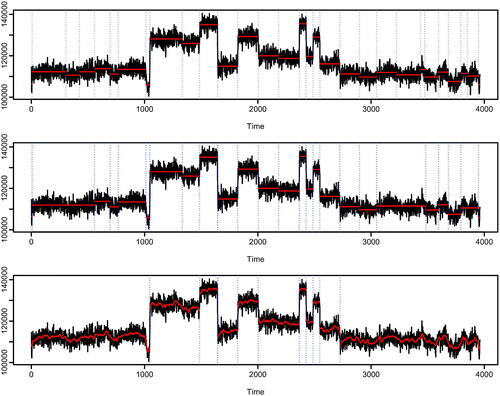
The top plot shows an analysis of the well-log data that uses wild binary segmentation (Fryzlewicz Citation2014) with the standard cusum test for a change in mean, and then estimates the number of changepoints based on a strengthened Schwarz information criteria. Both the cusum test and the strengthened Schwarz information criteria are based on modeling assumptions of a constant mean between changepoints and independent, identically distributed (IID) Gaussian noise, and are known to consistently estimate the number and location of the changepoints if these assumptions are correct. However, in this case, we can see that it massively overfits the number of changepoints. Similar results are obtained for standard implementation of other algorithms for detecting changes in mean, see Figure 13 in the supplementary material.
Lavielle and Moulines (Citation2000) and Bardwell et al. (Citation2019) suggested that if we estimate changepoints by minimizing the squared error loss of our fit with a penalty for each change, then we can correct for potential autocorrelation in the noise by inflating the penalty used for adding a changepoint. The middle plot of shows results for such an approach (Bardwell et al. Citation2019); this gives an improved result but it still noticeably overfits.
By comparison, the method we propose models both autocorrelation in the noise and local fluctuations in the mean between changepoints—and analysis of the data using default settings produces a much more reasonable segmentation of the data (see bottom plot of ). This method is model-based, and assumes that the local fluctuations in the mean are realizations of a random walk and that the noise process is an AR(1) process. We then segment the data by minimizing a penalized cost that is based on the log-likelihood of our model together with a BIC penalty for adding a changepoint.
The key algorithmic challenge with our approach is minimizing the penalized cost. In particular, many existing dynamic programming approaches (e.g., Jackson et al. Citation2005; Killick, Fearnhead, and Eckley Citation2012) do not work for our problem due to the dependence across segments caused by the autocorrelated noise. We introduce a novel extension of the functional pruned optimal partitioning algorithm of Maidstone et al. (Citation2017), and we call the resulting algorithm DeCAFS, for Detecting Changes in Autocorrelated and Fluctuating Signals. It is both computationally efficient (analysis of the approx 4000 data points in the well-log data taking a fraction of a second on a standard laptop) and guaranteed to find the best segmentation under our criteria.
While we are unaware of any previous method that tries to model both autocorrelation and local fluctuations, Chakar et al. (Citation2017) introduced AR1Seg which aims to detect changes in mean in the presence of autocorrelation. Their approach is similar to ours if we remove the random walk component, as they aim to minimize a penalized cost where the cost is the negative of the log-likelihood under a model with an AR(1) noise process. However they were unable to minimize this penalized cost, and instead minimized an approximation that removes the dependence across segments. One consequence of using this approximation is that it often estimates two consecutive changes at each changepoint, and AR1Seg uses a further post-processing step to try and correct this. Moreover, our simulation results show that using the approximation leads to a loss of power, particularly when the autocorrelation in the noise is high.
Particularly if interest lies in estimating how the underlying mean of the data varies over time, natural alternatives to DeCAFS are trend filtering methods (Kim et al. Citation2009; Tibshirani et al. Citation2014) which estimate the mean function under an L1 penalty on a suitably chosen discrete derivative of the mean. Depending on the order of the derivative, these methods can fit a piecewise constant (in this case trend filtering is equivalent to the fused lasso of Tibshirani et al. Citation2005), linear, or quadratic etc. function to the mean. One advantage of trend filtering is its flexibility: depending on the application one can fit mean functions with different degrees of smoothness. However, it does not allow one to jointly estimate a smoothly changing mean and abrupt changes—the L1 penalty must be chosen to capture one or other of these effects. This is particularly an issue if the main interest is in detecting abrupt changes rather than estimating the mean. These issues are investigated empirically in Appendix F.3.
Distinguishing between local fluctuations and abrupt changes is possible by methods that model the mean as a sum of functions (Jalali, Ravikumar, and Sanghavi Citation2013)—for example one smoothly varying and one piecewise constant. And trend-filtering, or other regularized estimators can then be used to estimate each component. The LAVA approach of Chernozhukov, Hansen, and Liao (Citation2017) is one such approach, fitting the piecewise constant function and the smoothly varying function using, respectively, an L1 and L2 penalty on the function’s first discrete derivative. The main difference between LAVA and DeCAFS is thus that LAVA has an L1 penalty for abrupt changes, and DeCAFS has an L0 penalty. If interest is primarily in detecting changes, previous work has shown the use of an L0 penalty to be preferable to an L1 penalty – as the latter can often over-fit the number of changes (see, e.g., the empirical evidence in Fearnhead, Maidstone, and Letchford Citation2018; Jewell et al. Citation2020), and a post-processing step is often needed to correct for this (Lin et al. Citation2017; Safikhani and Shojaie Citation2020).
One important feature of modeling the random fluctuations in the mean via a random walk, is that the information that a data point ys
has about a change at time t decays to 0 as gets large. This is most easily seen if we consider applying DeCAFS to detect a single abrupt change. We show in Section 5 that whether DeCAFS detects a change at a time t depends on some contrast of the data before and after t. This contrast compares a weighted mean of the data before t to a weighted mean of the data after t, with the weights decaying (essentially) geometrically with the length of time before/after t. This is appropriate for the random walk model which enables, for example, the mean of
to be very different to the mean at
if h > 0 is large, and thus
contains little to no information about whether there has been an abrupt change in the mean of
compared to the mean of yt
. By contrast, standard CUSUM methods for detecting a change in mean quantify the evidence for a change at t by a contrast of the unweighted mean of the data before and after t – thus each data point,
, has the same amount of information about the change regardless of the value of h. In situations where there are local fluctuations in the mean but through some stationary process, such as a mean-reverting random walk, data far from a change would still have a non-negligble amount of information about it. In such situations, particularly if the segments are long, DeCAFS could have lower power than CUSUM or other methods that ignore any local fluctuations in the data. We investigate this empirically in Appendix F.4.
The outline of the article is as follows. In the next section, we introduce our model-based approach and the associated penalized cost. In Section 3 we present DeCAFS, a novel dynamic programming algorithm that can exactly minimize the penalized cost. To implement our method we need estimates of the model parameters, and we present a simple way of preprocessing the data to obtain these in Section 4. We then look at the theoretical properties of the method. These justify the use of the BIC penalty, show that our method has more power at detecting changes when our model assumptions are correct than standard approaches, and also that we have some robustness to model error—in that we can still consistently estimate the number and location of the changepoints in such cases by adapting the penalty for adding a changepoint. Sections 6 and 7 evaluate the new method on simulated and real data; and the article ends with a discussion.
Code implementing the new algorithm is available in the R package DeCAFS on CRAN. The package and full code from our simulation study is also available at github.com/gtromano/DeCAFS.
2 Modeling and Detecting Abrupt Changes
2.1 Model
Let be a sequence of n observations, and assume we wish to detect abrupt changes in the mean of this data in the presence of local fluctuations and autocorrelated noise. We take a model-based approach where the signal vector is a realization of a random walk process with abrupt changes, and we super-impose an AR(1) noise process.
So for ,
(1)
(1) where for
(2)
(2)
and
except at time points immediately after a set of m changepoints,
. That is
unless
for some j. This model is unidentifiable at changepoints. If τ is a changepoint, then whilst the data is informative about
and
, we have no further information about the specific value of
relative to
. We thus take the convention that
and
, which is the most likely value of
under our model, and consistent with maximizing the likelihood criteria we introduce below. The noise process, ϵt
is a stationary AR(1) process with, for
,
(3)
(3)
for some autocorrelation parameter,
with
and
Special cases of our model occur when
or when
. When
our noise process ϵt
is then IID, and the model is equivalent to a random walk plus noise with abrupt changes. When
we are detecting changes in mean with an AR(1) noise process, resulting in a formulation equivalent to the one of Chakar et al. (Citation2017).
2.2 Penalized Maximum Likelihood Approach
In the following, we will assume that and
are known; we consider robust approaches to estimate these parameters from the data in Section 4. We can then write down a type of likelihood for our model, defined as the joint density of the observations,
, and the local fluctuations in the mean,
. We will express this as a function of
and
. Writing
for a generic conditional density, we have that this is
We have used the specific Gaussian densities of our model, and dropped multiplicative constants, to get the second expression.
If we knew the number of changepoints, then we could estimate their position by maximizing this likelihood subject to the constraints on the number of nonzero entries of . However, as we need to also estimate the number of changepoints we proceed by maximizing a penalized version of the log of the likelihood where we introduce a penalty for each changepoint—this is a common approach to changepoint detection, see, for example, Maidstone et al. (Citation2017). It is customary to restate this as minimizing a penalized cost, rather than maximizing a penalized likelihood, where the cost is minus twice the log-likelihood. That is, we estimate the number and location of the changepoints by solving the following minimization problem:
(4)
(4) where
is the penalty for adding a changepoint,
, and
is an indicator function. For the special case of a constant mean between changepoints, corresponding to
, we require
and simply drop the first term in the sum.
2.3 Dynamic Programming Recursion
We will use dynamic programming to minimize the penalized cost EquationEquation (4)(4)
(4) . The challenge here is to deal with the dependence across changepoints due to the AR(1) noise process which means that some standard dynamic approaches for change-point detection, such as optimal partitioning (Jackson et al. Citation2005) and PELT (Killick, Fearnhead, and Eckley Citation2012), cannot be used. To overcome this, as in Rigaill (Citation2015) or Maidstone et al. (Citation2017), we define the function
to be the minimum penalized cost for data
conditional on
,
So ; and the following proposition gives a recursion for
.
Proposition 1.
The set of functions satisfies
(5)
(5)
The intuition behind the recursion is that we first condition on , with the term in braces being the minimum penalized cost for
given u and
, and then minimize over u. The cost in braces is the sum of three terms: (i) the minimum penalized cost for
given u; (ii) the cost for the change in mean from u to μ; and (iii) the cost of fitting data point yt
with μt
. The cost for the change in mean, (ii), is just the minimum of the constant cost for adding a change and the quadratic cost for a change due to the random walk. The recursion applies to the special case of a constant mean between changepoints, where
, if we replace
with its limit as
, which is
.
Although recursions of this form have been considered in earlier changepoint algorithms (e.g., Maidstone et al. Citation2017; Hocking et al. Citation2020), the dependence between the current mean u and the previous mean μ that appears in terms (ii) and (iii) makes our recursion more challenging to solve. We next show one efficient way of solving by combining existing functional pruning dynamic programming ideas with properties of infimal convolutions.
3 Computationally Efficient Algorithm
3.1 The DeCAFS Algorithm
Algorithm 1 gives pseudo code for solving the dynamic programming recursion introduced in Proposition 1. The key to implementing this algorithm is performing the calculations in line 5, and how this can be done efficiently will be described below. Throughout we give the algorithm for the case where there is a random walk component, that is, , though it is trivial to adapt the algorithm to the
case.
As well as solving the recursion for , Algorithm 1 shows how we can also obtain the estimate of the mean, through a standard back-tracking step. The idea is that our estimate of μn
,
, is just the value of μ that maximizes
. We then loop backwards through the data, and our estimate of μt
is the value that minimizes the penalized cost for the data
conditional on
, which can be calculated as
in line 11.
Finally, as we obtain the estimates of the mean, we can also directly obtain the estimated changepoint locations. It is straightforward to see, by examining the form of the penalized cost, that the optimal solution for has
(and hence, t is a changepoint) if and only if
.
Algorithm 1: DeCAFS
Data: a time series of length n
Input: and
.
1 begin Initialization
2
3 end
4 for t = 2 to n do
5
6 end
7 begin Backtracking
8
9
10 for to 1 do
11
12
13 if then
14
15 end
16 end
17 end
18 Return
3.2 The Infimal Convolution
The main challenge with Algorithm 1 is implementing line 5. First, this needs a compact way of characterizing . This is possible as
is a quadratic function; and the recursion maps piecewise quadratic functions to piecewise quadratic functions. Hence
will be piecewise quadratic and can be defined by storing a partition of the real-line together with the coefficients of the quadratics for each interval in this partition.
Next we can simplify line 5 of Algorithm 1. As written line 5 involves minimizing a two-dimensional function, in , over the variable u. We can recast this operation into a one-dimensional problem by introducing the concept of an infimal convolution (see Chapter 12 of Bauschke and Combettes Citation2011).
Definition 1.
Let f be a real-valued function defined on and ω a nonnegative scalar. We define
and for
,
(6)
(6) as the infimal convolution of f with a quadratic term.
The following proposition presents a reformulation of the update-rule into a minimization involving infimal convolutions, for the case . The proof is in Appendix B, together with details of equivalent results when
.
Proposition 2.
Assume . The functions
can be written as
where
and
3.3 Fast Infimal Convolution Computation
As noted above we can represent Qt
by where each
is a quadratic defined on some interval
with
and
. It is this representation of Qt
that we update at each time step. Some operations involved in solving the recursion, such as adding a quadratic to a piecewise quadratic, or calculating the pointwise minimum of two piecewise quadratics are easy to perform with a computational cost that is linear in the number of intervals (see, e.g., Rigaill Citation2015). The following theorem shows that a fast update for the infimal convolution of a piecewise quadratic is also possible, and is important for developing a fast algorithm for solving the dynamic programming recursions.
Theorem 1.
Let be the representation of the functional cost Qt
. For all
, the representation returned by the infimal convolution
has the following order-preserving form:
with
and
.
The key part of this result is that the order of the quadratics is not changed when we apply the infimal convolution, and thus we can calculate using a linear scan over the real-line. The proof of this theorem is given in Appendix C, and an example algorithm for calculating
with complexity that is linear in s is shown in Appendix D.
4 Robust Parameter Estimation
Our optimization problem EquationEquation (4)(4)
(4) depends on three unknown parameters:
and
. We estimate these parameters by fitting to robust estimates of the variance of the k-lag differenced data,
Z
, for
.
Proposition 3.
With the model defined by EquationEquations (1)–(3),
Providing k is small relative to the average length of a segment, the mean of will be zero for most t: if there are m changes then at most km of the
’s will overlap a change and have a nonzero mean. This suggests that we can estimate the variance of
using a robust estimator, such as the median absolute difference from the median, or MAD, estimator.
Fix K, and let vk
be the MAD estimator of the variance of for
. We estimate the parameters by minimizing the least-square fit to these estimates,
In practice, we can minimize these criteria by using a grid of values for and then for each
value analytically minimize with respect to
and
. Obviously, if we are fitting a model without the random walk component, then we can set
, or if we wish to have uncorrelated noise, then we set
.
An empirical evaluation of this method for estimating the parameters is shown in Section F of the supplementary material. These include an investigation of the accuracy in situations where we have changepoints. In our simulation study, we use K = 10, though similar results were obtained as we varied K.
5 Theoretical Properties
We can reformulate our model as a linear-regression. To do this it is helpful to introduce new variables, , that give the cumulative effect of the random-walk fluctuations. To simplify exposition, it is further helpful to define this process so it has an invertible covariance matrix. So we will let
and
for
. For a set of m changepoints
, and defining
, we can introduce a
matrix
where the ith column is a column of
zeros followed by
ones. Our model is then
(7)
(7) where
is a vector of Gaussian random variables with
the sum of the variance matrices for the AR component of the model,
, and the random walk component of the model,
; and Δ is a
vector whose first entry is
and whose ith entry is
the change at the
th changepoint. This formulation allows us to consider the impact of model error on DeCAFS. Later, when we consider its asymptotic properties, we will allow for the data-generating process to be EquationEquation (7)
(7)
(7) but with
different from that assumed by DeCAFS.
As shown in Section E of the supplementary material, the unpenalized version of the cost that we minimize, conditional on a specific set of changepoints, can be written aswhere
is assumed to be a column vector. Thus, the penalized cost EquationEquation (4)
(4)
(4) is
. In the remainder of this section, we will call
the cost, and
the penalized cost.
While our cost is obtained by minimizing over , the following result shows that it is equal to the weighted residual sum of squares from fitting the linear model defined in EquationEquation (7)
(7)
(7) .
Proposition 4.
The cost for fitting a model with changepoints, is
(8)
(8)
Let denote the cost if we fit a model with no changepoints. The following corollary, which follows from standard arguments, gives the behavior of the cost under a null model of no changepoints. This includes a bound on the impact of mis-specifying the covariance matrix, for example due to mis-estimating the parameters of the AR(1) or random walk components of the model, or if our model for the residuals is incorrect.
Corollary 1.
Assume that data is generated from the model defined in EquationEquation (7)(7)
(7) , with m = 0 but with
a mean-zero Gaussian vector with
. Let
be the largest eigenvalue of
. If
then
. Otherwise, for any x
Furthermore, if we estimate the number of changepoints using the penalized cost EquationEquation (4)(4)
(4) with penalty
for any C > 2, then the estimated number of changepoints,
, satisfies
as
.
To gain insight into the behavior of the procedure in the presence of changepoints, and how it differs from standard standard change-in-mean procedures, it is helpful to consider the reduction in cost if we add a single changepoint.
Proposition 5.
Given a fixed changepoint location τ1:
The reduction in cost for adding a single changepoint at τ1 can be written as
, for some vector v defined as
where u0 is a column vector of n ones,
The vector v in (i) satisfies
For any vector w that satisfies
The vector v in part (i) of this proposition defines a projection of the data that is used to determine whether to add a changepoint at τ1. The properties in part (ii) mean that this projection is invariant to shifts of the data, and that the distribution of the reduction in cost if our model is correct and there are no changes will be . The statistic
can be viewed as analogous to the cusum statistic (Hinkley Citation1971) that is often used for a standard change-in-mean problem, and in fact if we set
and
so as to remove the auto regressive and random-walk aspects of the model,
is just the standard cusum statistic. The power of our method to detect a change at τ1 will be governed by the distribution of this projection applied to the data in the segments immediately before and after τ1. For a single changepoint where the mean changes by δ this distribution is a noncentral chi-squared with 1 degree of freedom and noncentrality parameter
. Thus, part (iii) shows that v is the best linear projection, in terms of maximizing the non-centrality parameter, over all projections that are invariant to shifts in the data and that are scaled so that the null distribution is
.
To gain insight into how the auto regressive and random-walk parts of the model affect the information in the data about a change we have plotted different projections v for different model scenarios in the top row of . The top-left plot shows the projections if we have for different, values of the random walk variance. The projection, naturally, places more weight to data near the putative changepoint, and the weight decays essentially geometrically as we move away from the putative changepoint. In the top-right plot we show the impact of increasing the autocorrelation of the AR(1) process, with the absolute value of the weight given to data points immediately before and after the putative change increasing with
.
Fig. 2 Top row: projections of data v for detecting a change in the middle of n = 100 data-points. Random walk model (top-left) for varying of 0.03 (black), 0.02 (red) and 0.01 (green); AR(1) plus random walk model (top-right) for
and varying
of 0.4 (black), 0.2 (red) and 0.1 (green). In both plots the blue line shows the standard cusum projection. Bottom row: noncentrality parameter for a
test of a change using the optimal projection (solid line) and the cusum projection (dashed line) for a change of size 1 in the middle of the data as we vary n. Out-fill asymptotics (bottom-left) where
is (0.0025,0) (black), (0.01,0) (red), (0.0025,0.5) (green) and (0.01,0.5) (blue); In-fill asymptotics (bottom-right) where for n = 50
is (0.0025,0) (black), (0.01,0) (red), (0.0025,0.5) (green) and (0.01,0.5) (blue).
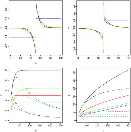
A key feature of the random walk model is that for any fixed the amount of information about a change will be bounded as we increase the segment lengths either side of the change. This is shown in the bottom-left plot of where we show the noncentrality parameter for detecting a change in the middle of the data as we vary n. For comparison we also show the non-centrality parameter of a test based on the cusum statistic (scaled so that it also has a
distribution under the null of no change). We can see that ignoring local fluctuations in the mean, if they exist and come from a random walk model, by using the cusum statistic leads to a reduction of power as segment lengths increase. For comparison in the bottom right we show an equivalent comparison where we consider an infill asymptotic regime, so that as n increases we let the random walk variance decay at a rate proportional to
and we increase the lag-1 autocorrelation appropriately. In this case using the optimal projection gives a noncentrality parameter that increases with n, whereas the cusum statistic has power that can be shown to be bounded as we increase n.
We now turn to the property of our method at detecting multiple changes. Based on the above discussion, we will consider in-fill asymptotics as .
(C1) Let
(C2) Assume there exists strictly positive constants
(C3) There exists an α such that for any large enough n if
The two regimes covered by condition C2 are due to the different limiting behavior of an AR(1) model under in-fill asymptotics, depending on whether the AR(1) noise is independent, case (i), or there is autocorrelation, case (ii). The form of in each case ensures that the AR(1) process has fixed marginal variance,
, for all values of n.
The key condition here is (C3) which governs how accurate the model assumed by DeCAFS is to the true data-generating procedure. Clearly, if the model is correct then (C3) holds with α = 1. The following proposition gives upper bound on α in the case where the covariance of the data-generating model is that of a random walk plus AR(1) process, but with different parameter values to those assumed by DeCAFS in (C2), for example, due to misestimation of these parameters.
Proposition 6.
Assume the noise process of the data-generating process (C1) is equal to a random walk plus an AR(1) process.
If
If
The following result shows that we can consistently estimate the number of changepoints and gives a bound on the error in the estimate of changepoint locations, if we use DeCAFS under an assumption of a maximum number of changepoints (the assumption of a maximum number changes is for technical convenience, though is common in similar results, e.g., Yao Citation1988).
Theorem 2.
Assume data, , is generated as described in (C1), and let
and
be the estimated number and location of the changepoints from DeCAFS implemented with parameters given by (C2), penalty
for some C > 2, and a maximum number of changes
. Then as
: if
and if
The most striking part of this result is the very different behavior between and
. In the latter case, asymptotically we detect the position of the changepoints without error. This is because the positive autocorrelation in the noise across the changepoint helps us detect it. In fact, as
the signal for a change at t comes just from the lag-1 difference,
. The variance of
is
, and its mean is 0 except at changepoints, where it takes a fixed non-zero value. A simple rule based on detecting a change at t if and only if
is above some threshold,
for some suitably large constant c1, would consistently detect the changes. For the infill asymptotics, we consider, empirically DeCAFS converges to such an approach as
.
The theorem also gives insight into the choice of penalty β. It is natural to choose this to be the smallest value that ensures consistency, as larger values will mean loss of power for detecting changes. Assuming the DeCAFS model is correct and we have the true hyper parameters this suggests using , the infimum of the penalties that are valid according to the theorem. This is the value that we use within our simulation study—though slightly inflating the penalty may be beneficial to account for error in the estimated hyper parameters or if we want to account for substantial model error.
6 Simulation Study
6.1 Comparison with Changepoint Methods
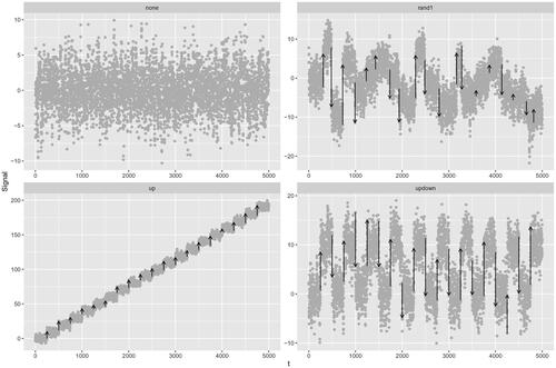
We now asses the performance of our algorithm in a simulation study on four different change scenarios, illustrated in . In all cases we run DeCAFS with , and estimate the parameters
as described in Section 4.
Fig. 3 Four different change scenarios. Top-left, no change present, top-right, change pattern with 19 different changes, bottom-left up changes only, bottom-right, up-down changes of the same magnitude. In this particular example data were generated from an AR model with .
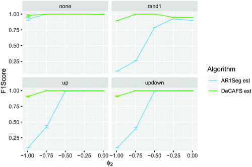
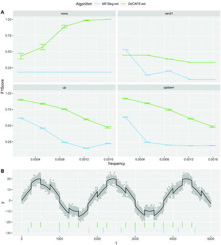
Simulations were performed over a range of evenly spaced values of . There are no current algorithms that directly model local fluctuations in the mean, so we compare with two approaches the assume a constant mean between changes: FPOP (Maidstone et al. Citation2017) which also assumes IID noise, and AR1Seg (Chakar et al. Citation2017) that models the noise as an AR(1) process. We compare default implementation of each method, which involves robust estimates of the assumed model parameters. We also compare an implementation of FPOP with an inflated penalty (Bardwell et al. Citation2019) to account for the autocorrelated noise. To see the impact of possible misestimation of the model parameters, we also implement DeCAFS and AR1Seg using the true parameters when this is possible.
We focus on the accuracy of these methods at detecting the changepoints. We deem a predict change as correct if it is within ±2 observations of a true changepoint. As a measure of accuracy we use the F1 score, which is defined as the harmonic mean of the precision (the proportion of detected changes that are correct) and the recall (the proportion of true changes that are detected). The F1 score ranges from 0 to 1, where 1 corresponds to a perfect segmentation. Separate figures for precision and recall can be found in Section G of the supplementary material. Results reported are based over 100 replications of each simulation experiment, with each simulated data having n = 5000.
In , we report performances of the various algorithms as we vary for fixed values of
and
. In , we additionally fix
, but we vary the size of changes. In these cases, there is no random walk component and the model assumed by AR1Seg is correct.
Fig. 4 F1 Scores on the 4 different scenarios. In A a pure AR(1) over a range of values of , for fixed values of
and a change of magnitude 10. In B a pure AR(1) process with fixed
and changes in the signal of various magnitudes. In C the full model with
for a range of values of
. The gray line represents the cross-section between parameters values in A, B, and C. AR1Seg est. and DeCAFS est. refer to the segmentation of the relative algorithms with estimated parameters. Note, in B the results from DeCAFS and DeCAFS est overlap so only one line is visible. Other algorithms use the true parameter values.
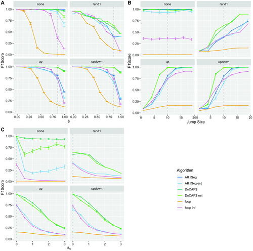
There are a number of conclusions to draw from these results. First, we see that the impact of estimating the parameters on the performance of DeCAFS and AR1Seg is small. Second, we see that using a method which ignores autocorrelation but just inflates the penalty for a change does surprisingly well unless the autocorrelation is large, , this is inline with results on the robustness of using a square error cost for detecting changes in mean (Lavielle and Moulines Citation2000). For high values of
, DeCAFS is the most accurate algorithm. The one exception are the simulations where there are no changes: the default penalty choice for AR1Seg is such that it rarely introduces a false positive.
In , we explore the effect of local fluctuations in the mean by varying . We see a quick drop off in performance for all methods as
increases, consistent with the fact that it is harder to detect abrupt changes when the local fluctuations of the mean are greater. Across all experiments, DeCAFS was the most accurate algorithm.
One word of caution when fitting the full DeCAFS model, is that when is large it can be difficult to estimate the parameters, as a model with a very high random walk variance produces data similar to that of a model with constant mean but high autocorrelation. Whilst the impact on detecting changes of any errors when estimating the parameters is small, it can lead to larger errors in the estimate of the signal, μt
: as different parameter estimates mean that the fluctuations in the data are viewed as either fluctuations in the noise process or in the signal. An example of this is shown in Section F of the supplementary material.
6.2 Robustness to Model Mis-specification
We now investigate the performance of DeCAFS when its model is incorrect. First we follow Chakar et al. (Citation2017) and simulate data with a constant mean between changes but with the noise process being AR(2), i.e. . In we report F1 Scores for DeCAFS and AR1Seg as we vary range
. Obviously as
increases, all algorithms perform worse, but the segmentations returned from DeCAFS are the more reliable as we increase the level of model error.
Fig. 5 F1 score on different scenarios with AR(2) noise as we vary . Data simulated fixing
and
over a change of size 20.
Second, we consider local fluctuations in the mean that are generated by a sinusoidal process rather than the random walk model, see . In , we compare performance of DeCAFS and AR1Seg as we vary the frequency of the sinusoidal process. Again we see that DeCAFS gives more reliable segmentations in these cases. In the three change scenarios performance decrease as we increase the frequency of the process. In these cases, it becomes significantly harder to detect any changepoints, however, DeCAFS still has higher scores than AR1Seg since it is more robust and returns fewer false positives.
Fig. 6 In A the F1Score on the 4 scenarios for the Sinusoidal Model for fixed amplitude of 15, changes of size 5 and IID Gaussian noise with a variance of 4, as we vary the frequency of the sinusoidal process. In B an example of a realization for the updown scenario, vertical segments refer to estimated changepoint locations of DeCAFS (in light green) and AR1Seg (in blue).
Additional simulation results, showing the robustness of DeCAFS to the mean fluctuations being from an Ornstein-Uhlenbeck process or to the noise being AR(1) within a segment but independent across segments are shown in Sections F and G in the Supplementary Material.
6.3 Comparison to LAVA
The LAVA method of Chernozhukov, Hansen, and Liao (Citation2017) can be applied to model a signal as the sum of a piecewise constant function and a locally fluctuating function: and is thus a natural alternative to DeCAFS. If we let X denote the n × n matrix whose ith column has i – 1 zeroes followed by ones then LAVA can estimate the mean
as
where the vectors f and g minimize
with
and
denoting, respectively, the L1 and L2 norms.
The interpretation of this is that is the change in the mean of the data from time i – 1 to time i. The penalties are such that
is sparse, and thus is modeling the abrupt changes in the mean, while
is dense and is accounting for the local fluctuations. It is possible to show that DeCAFS is equivalent to LAVA if we have independent noise and replace the L1 norm by an L0 norm.
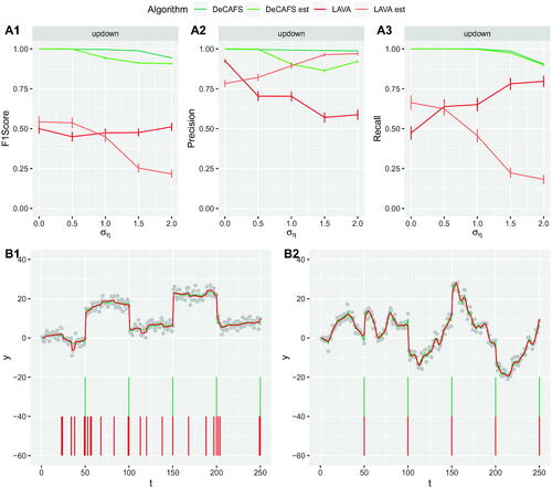
We implemented LAVA using the lavash package in R. This implementation of LAVA is substantially slower than DeCAFS, and empirically the computational cost appears to increase with the cube of the number of data points. As a result we compare DeCAFS with LAVA on simulated data of length n = 1000 (for which LAVA takes, on average, 132 seconds and DeCAFS 0.02 seconds per dataset).
LAVA tunes λ1 by cross-validation. We used a plug-in value for λ2 based on the oracle choice suggested in Chernozhukov, Hansen, and Liao (Citation2017). This choice depends on the variance of the local fluctuations, i.e. the variance of the random walk component in our model, and we implemented LAVA using both the true variance (denoted LAVA), and using the same estimate of the variance as we use for DeCAFS (denoted LAVA_est). The plug-in approach seemed to give better results, and was substantially faster than using cross-validation to tune λ2. It also makes a comparison with DeCAFS easier, as in situations where neither method estimates any abrupt changes, the two methods then give essentially identical estimates of the mean.
Results from analyzing data simulated under a pure random-walk model (so ) are shown in . While both methods perform similarly at estimating the underlying mean, we see that LAVA is less reliable at estimating the changepoint locations—and often substantially over-estimates the number of changepoints. As summarized in the introduction, this is not unexpected as it is common for methods that use
penalties on the size of an abrupt change to overestimate the number of changes (see, e.g., Fearnhead, Maidstone, and Letchford Citation2018; Jewell et al. Citation2020).
Fig. 7 On top: comparison of the F1 Score in A1, Precision in A2 and MSE in A3, for DeCAFS (in green) and LAVA (in red) with oracle initial parameters and the relative results with estimated initial parameters (in lighter colours), on the updown scenario for a random walk signal over a range of values of . On the bottom the first 250 observations of two realizations of the experiment with, in B1,
equal to 0.5 and in B2
equal to 2. Again, the continuous lines over the data points represent the signal estimates of DeCAFS and LAVA; and the vertical lines below show their estimated changepoint locations.
7 Gene Expression in Bacilus subtilis
We now evaluate DeCAFS on estimating the expression of cells in the bacteria Bacilus subtilis. Specifically, we analyze data from Nicolas et al. (Citation2009), which is data from tiling arrays with a resolution of less than 25 base pairs. Each array contains several hundred thousand probes which are ordered according to their position on the bacterial chromosome. For a probe, labeled t say, we get an RNA expression measure, Yt . shows data from 2000 probes. Code and data used in our analyses, presented below, are available on forgemia: https://forgemia.inra.fr/guillem.rigaill/decafsrna.
Fig. 8 Data on 2000 bp of the plus-strand of the Bacilus subtilis chromosome. Gray dots show the original data. The plain red line represents the estimated signal of DeCAFS with a penalty of . The dashed black line represents the estimated signal of hmmTiling.
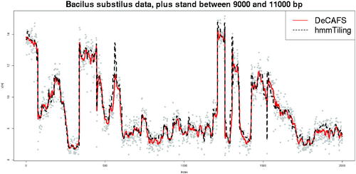
The underlying expression level is believed to undergo two types of transitions, large changes which Nicolas et al. (Citation2009) call shifts and small changes which they call drifts. Thus, it naturally fits our modeling framework of abrupt changes, the shifts, between which there are local fluctuations caused by the drifts. To evaluate the performance of DeCAFS at estimating how the gene expression levels vary across the genome we will compare to the hmmTiling method of Nicolas et al. (Citation2009). This method fits a discrete state hidden Markov model to the data, with the states being the gene expression level, and the dynamics of the hidden Markov model corresponding to either drifts or shifts. As a comparison of computational cost of the two methods, DeCAFS takes about 7 min to analyze data from one of the strands, each of which contains around 192,000 data points. Nicolas et al. (Citation2009) reported a runtime of 5 h and 36 min to analyze both strands.
A comparison of the estimated gene expression level from DeCAFS and from hmmTiling, for a 2000 base pair region of the genome, is shown in . We see a close agreement in the estimated level for most of the region, except for a couple of regions where hmmTiling estimates abrupt changes in gene expression level that DeCAFS does not.
To evaluate which of DeCAFS and hmmTiling is more accurate, we follow Nicolas et al. (Citation2009) and see how well the estimated gene expression levels align with bioinformatically predicted promoters and terminators. A promoter roughly corresponds to the start of a gene, and a terminator the end, and we expect gene expression to increase around a promoter and decrease around a terminator.
For promoters, consider all probe locations t from the tiling chip and consider a threshold parameter δ. We can count the number of probe locations with a predicted difference strictly greater than δ. We call this
Among those probes, we can count how many have a promoter nearby (within 22 base pairs). We call this
. By symmetry we can define an equivalent measure for terminators. A method is better than another if for the same
it achieves a larger
We used a data-driven approach to choose the penalty, β for DeCAFS, benefitting from having separate data from the plus and minus strand of the chromosome. For the penalty was learned on the minus strand data and tested on the plus strand data. More specifically we ran DeCAFS on the minus strand for For each β we computed
for a fixed
and took the β maximizing
:
for promoters and
for terminators.
Fig. 9 Benchmark comparisons. The number of promoters (left) and terminators (right) correctly predicted on the plus strand, using a 22 bp distance cutoff, as a function of the number of predicted breakpoints,
. Plain black lines are the results of hmmTiling (as reported in of Nicolas et al. Citation2009)). Dotted black lines are the results of hmmTiling when considering all probes rather than only those called transitions. Plain red lines are the results of DeCAFS using
for promoters and
for terminators. These values were learned on the minus strand using a data-driven approach. The thin dark-green leaning line represent
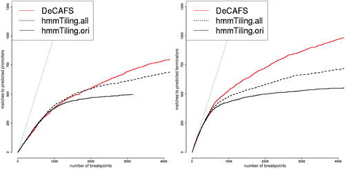
plots against
for the plus strand as we vary δ for DeCAFS and two different estimates from hmmTiling. The first, hmmTiling.ori, are the prediction presented in Nicolas et al. (Citation2009). The second, hmmtTiling.all, are those obtained when using all probes rather than only those called transitions by hmmTiling.
In the case of promoters, the prediction of hmmTiling is slightly better than DeCAFS for lower thresholds but noticeably worse for higher thresholds. In the case of terminators, the prediction of DeCAFS are clearly better than those of hmmTiling. Given that DeCAFS was not developed to analyze such data we believe that its relatively good performances for promoters and better performances for terminators is a sign of its versatility.
Unsurprisingly, we get different results and plots if we vary the value for used to select the penalty or if we use the plus strand as a training dataset and the minus strand as a testing dataset. However, Figure 16 in Appendix F.5 shows that
is robust to these choices and that the range of penalty for which DeCAFS is close to or better than hmmTiling is quite large, particularly for terminators.
8 Discussion
There are various ways of developing the DeCAFS algorithm, that build on other extensions of the functional pruning version of optimal partitioning. For example, to make the method robust to outliers, we can use robust losses, such as the bi-weight loss, instead of square error loss to measure our fit to the data (Fearnhead and Rigaill Citation2019). Alternatively, we can incorporate additional constraints on the underlying mean such as monotonicity (Hocking et al. Citation2020) or that the mean decays geometrically between changes (Jewell and Witten Citation2018; Jewell et al. Citation2020). Also it can be extended to allow for the noise to be independent across segments, but AR(1) within a segment. Finally, the algorithm is inherently sequential and thus should be straightforward to adapt to an online analysis of a data stream.
We do not claim that the method we present in Section 4 for estimating the parameters in our model is best. It is likely that more efficient or more robust methods are possible, for example using different robust estimates of the variances of the k-lag difference data (Rousseeuw and Croux Citation1993); or using iterative procedures where we estimate the changepoints, and then conditional on these changepoints re-estimate the parameters. Using better estimates should lead to further improvement on the statistical performance we observed in Section 6. Our theoretical results suggest that for estimating changes, mis-estimation of the parameters, or errors in our model for the noise or local fluctuations, can be corrected by inflating the penalty for adding a changepoint. As such, in applications we would suggest implementing the method for a range of penalty values, for example using the CROPS algorithm (Haynes, Eckley, and Fearnhead Citation2017), and then choosing the number of penalties using criteria that consider how the fit to data improves as we add more changes (e.g., Arlot et al. Citation2016; Fryzlewicz 2018 a; Arlot Citation2019); or use training data to evaluate performance for different values of β, as we did in Section 7.
Supplemental Material
Download PDF (2.9 MB)Acknowledgments
We thank Pierre Nicolas for providing the output of hmmTiling on the Bacillus subtilis data and his R code allowing us to generate , which closely resembles of Nicolas et al. (Citation2009).
Additional information
Funding
References
- Arlot, S. (2019), “Minimal Penalties and the Slope Heuristics: A Survey,” arXiv:1901.07277.
- Arlot, S., Brault, V., Baudry, J.-P., Maugis, C., and Michel, B. (2016), capushe: CAlibrating Penalities Using Slope HEuristics. R package version 1.1.1. https://CRAN.R-project.org/package=capushe
- Bardwell, L., Fearnhead, P., Eckley, I. A., Smith, S. and Spott, M. (2019), “Most Recent Changepoint Detection in Panel Data,” Technometrics, 61, 88–98. DOI: 10.1080/00401706.2018.1438926.
- Bauschke, H. H., and Combettes, P. L. (2011), Convex Analysis and Monotone Operator Theory in Hilbert Spaces, Vol. 408. Berlin: Springer.
- Chakar, S., Lebarbier, E., Lévy-Leduc, C., and Robin, S. (2017), ‘A Robust Approach for Estimating Change-points in the Mean of an AR(1) Process,” Bernoulli, 23, 1408–1447. DOI: 10.3150/15-BEJ782.
- Chernozhukov, V., Hansen, C. and Liao, Y. (2017), “A Lava Attack on the Recovery of Sums of Dense and Sparse Signals,” The Annals of Statistics, 45, 39–46. DOI: 10.1214/16-AOS1434.
- Eichinger, B., and Kirch, C. (2018), “A Mosum Procedure for the Estimation of Multiple Random Change Points,” Bernoulli, 24, 526–564. DOI: 10.3150/16-BEJ887.
- Fearnhead, P. and Liu, Z. (2011), “Efficient Bayesian Analysis of Multiple Changepoint Models With Dependence Across Segments,’’ Statistics and Computing, 21, 217–229. DOI: 10.1007/s11222-009-9163-6.
- Fearnhead, P., Maidstone, R. and Letchford, A. (2018), “Detecting Changes in Slope With an l 0 Penalty,” Journal of Computational and Graphical Statistics, 28, 265–275. DOI: 10.1080/10618600.2018.1512868.
- Fearnhead, P., and Rigaill, G. (2019), “Changepoint Detection in the Presence of Outliers,” Journal of the American Statistical Association, 114, 169–183. DOI: 10.1080/01621459.2017.1385466.
- Frick, K., Munk, A., and Sieling, H. (2014), “Multiscale Change-point Inference,” Journal of the Royal Statistical Society, Series B, 76, 495–580. DOI: 10.1111/rssb.12047.
- Fryzlewicz, P. (2014), “Wild Binary Segmentation for Multiple Change-Point Detection’, Annals of Statistics, 42, 2243–2281.
- Fryzlewicz, P. (2018a), “Detecting Possibly Frequent Change-points: Wild Binary Segmentation 2 and Steepest-drop Model Selection,” arXiv:1812.06880.
- Fryzlewicz, P. (2018b), “Tail-greedy Bottom-up Data Decompositions and Fast Multiple Change-point Detection,” The Annals of Statistics, 46, 3390–3421.
- Futschik, A., Hotz, T., Munk, A. and Sieling, H. (2014), “Multiscale DNA Partitioning: Statistical Evidence for Segments,” Bioinformatics, 30, 2255–2262. DOI: 10.1093/bioinformatics/btu180.
- Haynes, K., Eckley, I. A., and Fearnhead, P. (2017), “Computationally Efficient Changepoint Detection for a Range of Penalties,” Journal of Computational and Graphical Statistics, 26, 134–143. DOI: 10.1080/10618600.2015.1116445.
- Hinkley, D. V. (1971), “Inference About the Change-point From Cumulative Sum Tests,” Biometrika, 58, 509–523. DOI: 10.1093/biomet/58.3.509.
- Hocking, T. D., Rigaill, G., Fearnhead, P., and Bourque, G. (2020), “Constrained Dynamic Programming and Supervised Penalty Learning Algorithms for Peak Detection in Genomic Data,” Journal of Machine Learning Research, 21, 1–40.
- Hotz, T., Schütte, O. M., Sieling, H., Polupanow, T., Diederichsen, U., Steinem, C., and Munk, A. (2013), “Idealizing Ion Channel Recordings by a Jump Segmentation Multiresolution Filter,” IEEE Transactions on Nanobioscience, 12, 376–386. DOI: 10.1109/TNB.2013.2284063.
- Jackson, B., Scargle, J. D., Barnes, D., Arabhi, S., Alt, A., Gioumousis, P., Gwin, E., Sangtrakulcharoen, P., Tan, L. and Tsai, T. T. (2005), “An algorithm for Optimal Partitioning of Data on an Interval,” IEEE Signal Processing Letters, 12, 105–108. DOI: 10.1109/LSP.2001.838216.
- Jalali, A., Ravikumar, P., and Sanghavi, S. (2013), “A Dirty Model for Multiple Sparse Regression,” IEEE Transactions on Information Theory, 59, 7947–7968. DOI: 10.1109/TIT.2013.2280272.
- Jewell, S. W., Hocking, T. D., Fearnhead, P., and Witten, D. M. (2020), “Fast Nonconvex Deconvolution of Calcium Imaging Data,” Biostatistics, 21, 709–726. DOI: 10.1093/biostatistics/kxy083.
- Jewell, S., and Witten, D. (2018), ‘Exact Spike Train Inference Via l0 Optimization,” The Annals of Applied Statistics, 12, 2457–2482. DOI: 10.1214/18-AOAS1162.
- Killick, R., Eckley, I. A., Ewans, K., and Jonathan, P. (2010), “Detection of Changes in Variance of Oceanographic Time-series Using Changepoint Analysis,” Ocean Engineering, 37, 1120–1126. DOI: 10.1016/j.oceaneng.2010.04.009.
- Killick, R., Fearnhead, P., and Eckley, I. A. (2012), “Optimal Detection of Changepoints With a Linear Computational Cost,” Journal of the American Statistical Association, 107, 1590–1598. DOI: 10.1080/01621459.2012.737745.
- Kim, C.-J., Morley, J. C., and Nelson, C. R. (2005), “The Structural Break in the Equity Premium,” Journal of Business & Economic Statistics, 23, 181–191.
- Kim, S.-J., Koh, K., Boyd, S., and Gorinevsky, D. (2009), “l _1 Trend Filtering,” SIAM Review, 51, 339–360.
- Lavielle, M., and Moulines, E. (2000), “Least-squares Estimation of an Unknown Number of Shifts in a Time Series,” Journal of Time Series Analysis, 21, 33–59. DOI: 10.1111/1467-9892.00172.
- Lin, K., Sharpnack, J. L., Rinaldo, A. and Tibshirani, R. J. (2017), “A Sharp Error Analysis for the Fused Lasso, With Application to Approximate Changepoint Screening,” in Advances in Neural Information Processing Systems, eds. I. Guyon, U. V. Luxburg, S. Bengio, H. Wallach, R. Fergus, S. Vishwanathan and R. Garnett, Vol. 30, Red Hook, NY: Curran Associates Inc., 6884–6893.
- Maidstone, R., Hocking, T., Rigaill, G. and Fearnhead, P. (2017), “On Optimal Multiple Changepoint Algorithms for Large Data,” Statistics and Computing, 27, 519–533. DOI: 10.1007/s11222-016-9636-3.
- Nicolas, P., Leduc, A., Robin, S., Rasmussen, S., Jarmer, H., and Bessières, P. (2009), “Transcriptional Landscape Estimation From Tiling Array Data Using a Model of Signal Shift and Drift,” Bioinformatics, 25, 2341–2347. DOI: 10.1093/bioinformatics/btp395.
- Olshen, A. B., Venkatraman, E. S., Lucito, R., and Wigler, M. (2004), “Circular Binary Segmentation for the Analysis of Array-Based DNA Copy Number Data,” Biostatistics, 5, 557–572. DOI: 10.1093/biostatistics/kxh008.
- Reeves, J., Chen, J., Wang, X. L., Lund, R., and Lu, Q. Q. (2007), “A Review and Comparison of Changepoint Detection Techniques for Climate Data,” Journal of Applied Meteorology and Climatology, 46, 900–915. DOI: 10.1175/JAM2493.1.
- Rigaill, G. (2015), “A Pruned Dynamic Programming Algorithm to Recover the Best Segmentations With 1 to kmax Change-points,” Journal de la Societe Francaise de Statistique, 156, 180–205.
- Rousseeuw, P. J., and Croux, C. (1993), ‘Alternatives to the Median Absolute Deviation,” Journal of the American Statistical Association, 88, 1273–1283. DOI: 10.1080/01621459.1993.10476408.
- Ruanaidh, J. J. O., and Fitzgerald, W. J. (2012), Numerical Bayesian Methods Applied to Signal Processing, Springer Science & Business Media, New York: Springer-Verlag.
- Safikhani, A., and Shojaie, A. (2020), “Joint Structural Break Detection and Parameter Estimation in High-dimensional Non-stationary VAR Models,” Journal of the American Statistical Association, DOI: 10.1080/01621459.2020.1770097, 1–26.
- Tibshirani, R. J. et al. (2014), ‘Adaptive Piecewise Polynomial Estimation Via Trend Filtering,” The Annals of Statistics, 42, 285–323. DOI: 10.1214/13-AOS1189.
- Tibshirani, R., Saunders, M., Rosset, S., Zhu, J., and Knight, K. (2005), “Sparsity and Smoothness Via the Fused Lasso,” Journal of the Royal Statistical Society, Series B, 67, 91–108. DOI: 10.1111/j.1467-9868.2005.00490.x.
- Yao, Y.-C. (1988), ‘Estimating the Number of Change-points Via Schwarz’s Criterion,” Statistics & Probability Letters, 6, 181–189.