Earthquake Risk Embedded in Property Prices: Evidence From Five Japanese Cities

Abstract

We analyze the impact of short-run (90 days) and long-run (30 years) earthquake risk on real estate transaction prices in five Japanese cities (Tokyo, Osaka, Nagoya, Fukuoka, and Sapporo), using quarterly data over the period 2006–2015. We exploit a rich panel dataset (331,343 observations) with property characteristics, ward attractiveness information, macroeconomic variables, and long-run seismic hazard data, supplemented with short-run earthquake probabilities generated from a seismic excitation model using historical earthquake occurrences. We design a hedonic property price model that allows for subjective probability weighting, employ a multivariate error components structure, and develop associated maximum likelihood estimation and variance computation procedures. Our approach enables us to identify the total compensation for earthquake risk embedded in property prices, to decompose this into pieces stemming from short-run and long-run risk, and to distinguish between objective and subjectively weighted (“distorted”) earthquake probabilities. We find that objective long-run earthquake probabilities have a statistically significant negative impact on property prices, whereas short-run earthquake probabilities become statistically significant only when we allow them to be distorted. The total compensation for earthquake risk amounts to an average –2.0% of log property prices, slightly more than the annual income of a middle-income Japanese household. Supplementary materials for this article, including a standardized description of the materials available for reproducing the work, are available as an online supplement.

Keywords:

• Earthquake risk
• Hedonic pricing
• House price
• Multivariate error components
• Probability weighting
• Seismic excitation

1 Introduction

In Japan, earthquake risk is a reality. Every day in and around Japan, about three earthquakes occur with a magnitude of M > 4 on the Richter scale, and twice a month with a magnitude of M > 6. Earthquake risk varies, over days and between and within cities.

We are interested in analyzing the impact of natural catastrophe risk, Japanese earthquake risk in particular, on property valuation. We distinguish between different measures of earthquake risk. We consider long-run earthquake probabilities providing a stable objective measure of the average earthquake risk in a given (small) area in the next 30 years, and short-run earthquake probabilities providing an objective measure of local earthquake risk in the next 90 days. Objectively measured risk is, however, not the same as the perception and subjective evaluation of risk, and by transforming objective probabilities using subjective probability weighting we attempt to capture this. This article thus analyzes the subjective evaluation of both short- and long-run earthquake risk embedded in Japanese property prices. These property prices serve, in a sense, as a vehicle to statistically assess features of the human nature in relation to subjective risk evaluation.

Earthquakes tend to occur in clusters rather than in isolation. These seismic clusters may take the form of foreshocks and aftershocks anticipating and following a major earthquake or of a collection of major earthquakes triggering one another by causing frictions that put strain on neighboring faults. There is therefore objective predictive content embedded in the occurrence of earthquakes. This phenomenon is known as “seismic excitation” and there exists a large literature in statistics aimed at capturing it.

In a different strand of the literature in economics, several articles analyze the impact of natural catastrophes on property prices. Most commonly, this literature incorporates the prevailing binary state of the world, depending on whether or not a catastrophe has occurred, into a hedonic house price model of the Rosen (1974) type, which has become the benchmark model in analyzing property prices. Within a typical hedonic price model, the characteristics of a property are viewed as detachable components that each contribute to a part of the property price. The selection of components ranges from traditional house attributes such as square footage, location and building age, to external factors such as macroeconomic effects. The negative effect coming from hazardous environmental events, such as flood, hurricane and earthquake, has been addressed by various researchers; see, among others, Brookshire et al. (1985), Kawawaki and Ota (1996), Beron et al. (1997), Yamaga, Nakagawa, and Saito (2002), Bin and Polasky (2004), Nakagawa, Saito, and Yamaga (2007), Nakagawa, Saito, and Yamaga (2009), Daniel, Florax, and Rietveld (2009), Naoi, Seko, and Sumita (2009), Naoi, Seko, and Ishino (2012), Gu et al. (2011), Bin and Landry (2013), Hidano, Hoshino, and Sugiura (2015), and Hanaoka, Shigeoka, and Watanabe (2018).

In recent years, a large body of literature has documented, empirically, that people do not typically treat objective probabilities in a linear fashion, but rather tend to overweight small probability events and underweight large probability events. This is particularly relevant when evaluating catastrophic events that are often of a low-probability high-impact nature. Various modern theories of decision under risk, such as rank-dependent utility theory (Quiggin 1982) and prospect theory (Tversky and Kahneman 1992), feature a probability weighting function that “distorts” objective probabilities.

In this article, we introduce into a hedonic price model an objective measure of seismic excitation, next to a more conventional measure of long-run earthquake risk, and allow for probability weighting in the spirit of the nonexpected utility theories of rank-dependent utility and prospect theory. We use a rich panel dataset containing property characteristics, ward attractiveness information, macroeconomic variables, seismic hazard data, and historical earthquake occurrences. We design a hedonic price model with a multivariate error components structure (Baltagi 1980, 2008; Magnus 1982) for which we develop associated maximum likelihood estimation and variance computation procedures. By exploiting the matrix form of the error components, we are able to estimate the model while pooling properties of different types together, in spite of the very large dimension of the variance matrix and the fact that each property type corresponds to different features and total price levels. Our approach allows us to isolate the total compensation for earthquake risk embedded in Japanese property prices, and to decompose this into pieces stemming from short-run risk and long-run risk, and a further decomposition into objective and distorted risk components.

The occurrences of major earthquakes have served previously in hedonic price models with regression discontinuity design as natural exogenous events to elicit causal pricing effects. Limitations of this conventional approach include the purely binary nature of this treatment, which does not reflect the multiplicity of the events, the time elapsed since the last event, and the severity of the events. By contrast, our approach relies on a continuous-time predictive earthquake intensity that depends on all previous earthquakes, with recent ones being more important than older ones, and explicitly accounts for the severity of the events. Moreover, and at least equally importantly, this earthquake intensity can be translated into objective short-run probabilities enabling us to analyze probability weighting.

We can summarize our main findings as follows. First, we find that objective long-run earthquake risk has a significant negative impact on property prices, and increasingly so at higher risk levels. Second, given that long-run risk matters for property prices, we find that the additional impact of objective short-run earthquake risk on property prices, while estimated at negative values, is not significantly different from zero. Upon allowing for probability weighting, however, the distorted short-run earthquake probabilities do have a significantly negative effect on property prices. Third, the probability weighting function for short-run earthquake risk is found to be S-shaped, thus underweighting small probabilities and overweighting larger probabilities, contrary to the inverse-S shaped probability weighting function found in many experiments. This remarkable finding may be explained by the fact that the background arrival rate of earthquakes is positive rather than zero, in particular in Tokyo where the short-run earthquake probabilities never drop below 35% in the period that we analyze. Therefore, people may tend to evaluate and overweight temporary deviations of the short-run earthquake probabilities from the background seismicity caused by seismic excitation not with respect to zero but with respect to a positive reference probability level. In an extension of our base model, we also analyze probability distortions of long-run time-invariant earthquake probabilities. In this case, we find that small probabilities tend to be overweighted and large probabilities tend to be underweighted, in accordance with conventional wisdom.

Our work is related to the existing work on the interplay between property prices and environmental hazards cited above, and also to the financial econometrics literature on the estimation of risk and financial excitation premia embedded in asset and derivative prices; see Aït-Sahalia, Laeven, and Pelizzon (2014), Aït-Sahalia, Cacho-Diaz, and Laeven (2015), and Boswijk, Laeven, and Lalu (2016).

The remainder of this article proceeds as follows. Section 2 explains our treatment of objective seismic excitation and of probability weighting. Section 3 describes the dataset. Section 4 lays out our hedonic house price model with multivariate error components and Section 5 develops the procedures for estimation. Section 6 presents the estimation results. Section 7 considers an extension that also allows for probability distortions of long-run earthquake probabilities. Section 8 concludes.

This article comes with three supplementary files. First, the Appendix which contains various technical results, a discussion of the robustness of our estimation results, an analysis of the influence of each component to the total property prices and the implied premia for earthquake risk, a brief literature review, and an auxiliary figure. Second, the Data Documentation, which contains a detailed description of the data.¹ And third, the cleaned and compiled datasets and all codes to implement the procedures developed in this article, including our multivariate error components regression R package mvecr.²

2 Seismic Excitation and Probability Weighting

In this section, we develop a regression design that considers short-run earthquake probabilities as objective measures of seismic excitation, and allows for probability weighting.

2.1 Short-Run Earthquake Probabilities

Our approach estimates an epidemic-type aftershock sequence (ETAS) model and generates a panel of model-implied short-run earthquake probabilities which vary per quarter and per city, to be used in our regression design. These probabilities can be viewed as objective measures of short-run earthquake risk, summarizing publicly available information per time period and per city.

The ETAS model was introduced by Ogata (1988) and has since been widely used to capture the quiescence and activation of seismic dynamics. The basic idea of the model is that each earthquake can trigger a sequence of aftershocks like “epidemics” in that the occurrence of an earthquake makes future earthquakes more likely and that the impact of the trigger event diminishes over time (and distance). Despite the existence of several space-time extensions, we choose the temporal version of the ETAS model as described in the following, which we estimate separately for each of the five cities. Because we consider five cities this treatment is natural and simpler than first estimating a space-time version to a large area that covers all five cities and then isolating the city effects.

Formally, the ETAS model is a path-dependent marked point process and a special case of a Hawkes self-exciting process. Given observations of earthquake occurrences at times $t_1,t_2,\dots ,t_n$ over an interval $[0,T](T\ge t_n)$, the associated counting process N_t is defined as $N_t={\sum }_{i=1}^n{1}_{t_i\le t}$. Denoting by ${\mathcal{F}}_t$ the information filtration up to time t, the corresponding left-continuous ${\mathcal{F}}_t$-conditional jump intensity process λ_t describes the mean jump rate per unit of time,$${\lambda }_t=\lambda (t|{\mathcal{F}}_t)=\underset{h\downarrow 0}{\lim }\frac{1}{h}\mathrm{Pr}\left[N_{t+h}-N_t>0|{\mathcal{F}}_t\right].$$

In the temporal ETAS model, the conditional intensity function may be written as$${\lambda }_t={\lambda }_{\infty }+\sum _{t_i<t}c(m_i,m_c)g(t-t_i),$$where ${\lambda }_{\infty }>0$ (measured in number of jumps per time unit) is the background seismicity, $g(t-t_i)$ is the aftershock decay (i.e., time response) function, and the weight assigned to the aftershock decay is a function $c(m_i,m_c)$ of the magnitude of the earthquake m_i and a cutoff (i.e., threshold) magnitude m_c. Thus, the earthquake intensity depends on the background intensity and a weighted sum of all aftershock decays, where the sum is taken over all earthquakes that have occurred before time t. In the ETAS model, g takes the form of the so-called modified Omori law and c takes an exponential form.

We estimate the ETAS model for each of the five cities that we consider, based on the earthquake catalog of five areas covering the five cities, over the period January 1, 1970 to December 31, 2015. Next, we use the estimated intensities to generate, by simulation, 90-day probabilities of an earthquake exceeding a magnitude threshold of 5.5, for each city. Our simulation method follows Ogata (1981). We interpret these probabilities as measures of objective short-term seismic risk, impacting the prospective homeowner’s perception of seismic risk. We take the spatial windows somewhat larger than the city of interest, as seismic activity just outside the city may also impact the risk perception. Furthermore, this also helps to reduce the bias of the ETAS parameters stemming from seismicity originating outside of the extent of the spatial window; see Figure E1 in Appendix E (supplementary material). Further details about the parameterization, estimation, and simulation within the ETAS model are contained in our Data Documentation.

Fig. 1 Short-run earthquake risk: Simulated short-run earthquake probabilities and the logarithm of the earthquake intensity series for Tokyo. Events marked in the graph: ①: 2007-07-16 Chuetsu Offshore earthquake, $M6.8$. ②: 2009-08-09 Izu Islands earthquake, $M6.8$ and 2009-08-11 Shizuoka earthquake, $M6.5$. ③: 2011-03-11 Tohoku earthquake, $M9.0$. ④: 2012-01-01 Izu Islands, $M7.0$. ⑤: 2013-10-26 Fukushima-ken oki earthquake, $M7.1$. (Source: Japan Meteorological Agency, $M=\text{magnitude}$).

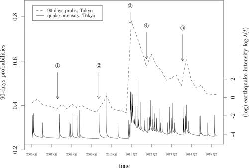
In Figures 1 and 2, we plot the earthquake intensities along with the corresponding short-run probability series for two of the five cities: Tokyo and Nagoya. The probabilities spike up immediately after a large earthquake and die out gradually until another major earthquake occurs. The Tohoku earthquake of Friday 11 March 2011 was the most powerful earthquake ever recorded in Japan. The spike is visible in 2011/Q2 (rather than in 2011/Q1), because the short-run probabilities are simulated based on actual earthquakes up to and including the previous quarter.

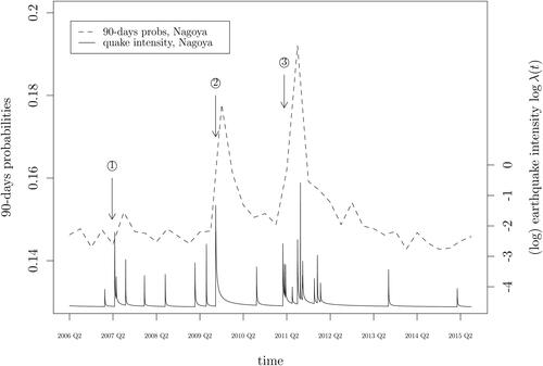
Fig. 2 Short-run earthquake risk: Simulated short-run earthquake probabilities and the logarithm of the earthquake intensity series for Nagoya. Events marked in the graph: ①: 2007-03-25 Noto Hanto earthquake, $M6.9$. ②: 2009-08-11 Shizuoka earthquake, $M6.5$. ③: 2011-03-11 Tohoku earthquake, $M9.0$. (Source: Japan Meteorological Agency).

The objective measure of seismic excitation given by the 90-day earthquake probabilities is included in our regression design. The rationale is that, in addition to the long-run earthquake risk that people may take into consideration when purchasing a property, news from a recent nearby earthquake may also temporarily affect property prices. Just like objective seismic excitation generated by a self-exciting process, the impact of such bad news on the people’s perception of risk peaks right after the event and dies out as time proceeds.

2.2 Probability Weighting

To account for probability weighting, our regression design furthermore allows for a parametric probability weighting function. There is a large literature on probability weighting. Probability weighting is an important ingredient of prospect theory (Kahneman and Tversky 1979; Tversky and Kahneman 1992), and of the related decision theories given by the dual theory of choice under risk (Yaari 1987) and rank-dependent utility (Quiggin 1982), which are building blocks of prospect theory.

We shall consider two canonical one-parameter families of probability weighting functions, proposed by Tversky and Kahneman (1992) and Prelec (1998), respectively. The Tversky-Kahneman function—see also Wu and Gonzalez (1996)—is given by(1) $$w(p)=\frac{p^{\psi }}{{(p^{\psi }+{(1-p)}^{\psi })}^{1/\psi }},$$(1) while the Prelec function is given by(2) $$w(p)=e^{-{(-\hspace{0.17em}\text{log}\hspace{0.17em}p)}^{\psi }}.$$(2)

The parameter ψ is restricted to be positive. When $0.279<\psi <1$ the Tversky-Kahneman function is inverse S-shaped, while the Prelec function is inverse S-shaped for $0<\psi <1$; when ψ = 1 both functions reduce to w(p) = p; and when $\psi >1$ both functions are initially S-shaped, but (only) the Tversky-Kahneman function becomes convex for large values of ψ. These two parametric families of probability weighting functions are the two most widely used models of probability weighting in economics and decision sciences. Together they allow for wide variation in the shape of the probability weighting function, so we can let the data speak for themselves in the current context.

In laboratory experiments (see Wu and Gonzalez 1996; Abdellaoui 2000), the probability weighting function is often found to be inverse S-shaped, first concave and then convex. An inverse S-shape captures the phenomenon that people tend to become less sensitive to changes in objective probabilities as these probabilities move further away from the reference point 0 and become more sensitive as they get closer to the reference point 1. The inverse S-shape is consistent with a positive third derivative of the probability weighting function. The interpretation of the signs of the successive derivatives of the probability weighting function was recently provided by Eeckhoudt, Laeven, and Schlesinger (2020). Note that contrary to the Tversky-Kahneman function the Prelec function has an invariant fixed point and inflection point at $p=1/e=0.37$, which implies that it can never be globally convex or concave.

3 The Data

The data collection process for this project has been complex and elaborate, and in this section we provide a brief summary. Full details and references to sources are available in our Data Documentation. We are interested in the impact of earthquake risk on property prices in major cities in Japan, and we have selected five cities for our purpose. Each city is divided into wards and each ward is divided into districts. (In the original dataset the word “area” is used. We prefer “district” to avoid confusion with other uses of the word “area.”) Certain information that can affect (and explain/predict) the attractiveness of buying a property is available per ward. For example, population characteristics, information about schools and medical facilities, shopping, safety, etc. We distinguish between three types of properties: “residential land (land and building),” “residential land (land only),” and “pre-owned condominiums” (hereafter, condos). Sales prices and property characteristics are available for each of these types in each of the five cities. We do not know the exact location of a property, but we do know in which district the property lies and we also know the distance to the nearest station and the name of that station. Some macro variables are relevant and affect house prices nationally. Finally, we have information on historical earthquake data and on earthquake risk data.

Cities

Japan has 12 cities with a population of more than one million people. Almost 100 million people, or 78% of the country’s total population of 127.4 million, live in urban areas. The total population of Japan’s largest 103 cities amounts to 63.9 million or just over half of all the country’s residents. Tokyo, with almost nine million inhabitants, is by far the largest Japanese city. (Strictly speaking, Tokyo is not a city—it is a prefecture, but we shall call it a city.) With a population of 3.7 million, Yokohama, south of Tokyo, is the Japan’s second largest city. Osaka and Nagoya are Japan’s third and fourth cities, each with a population of over two million. Eight cities have between one and two million inhabitants: Sapporo, Kobe, Fukuoka, Kyoto, Kawasaki, Saitama, Hiroshima, and Sendai.

From these 12 cities, we selected five: Tokyo, Osaka, Nagoya, Fukuoka, and Sapporo. This choice guarantees that each of the three major metropolitan areas is represented: the greater Tokyo area (Tokyo, Yokohama, Kawasaki, and Saitama) by Tokyo, the Kansai region (Osaka, Kobe, and Kyoto) by Osaka, and the Chukyo metropolitan area by Nagoya. To obtain a representative geographical spread we added Sapporo, the largest city in the North, and Fukuoka, the second largest city in the West after Osaka. Data limitations prevented us from including Hiroshima, while Sendai was not included because it is too close to Fukushima where the 2011 nuclear disaster took place following the Tohoku earthquake.

Wards

A designated city is a Japanese city that has a population greater than 500,000 and has been designated as such by order of the Cabinet of Japan. Designated cities are delegated many of the tasks normally performed by prefectural governments, such as public education, social welfare, sanitation, business licensing, and urban planning. Designated cities are required to subdivide themselves into wards (“ku”), each of which has a ward office conducting various administrative functions for the city government. The 23 special wards of Tokyo are not part of this system, as Tokyo is a prefecture, and its wards are effectively independent cities. The five cities together contain 80 wards (regular and special together): 23 in Tokyo, 24 in Osaka, 16 in Nagoya, 7 in Fukuoka, and 10 in Sapporo.

When considering to buy a property in a given city, one is likely to be interested in certain characteristics of these wards. The original dataset contains one hundred characteristics divided into 11 categories. Since many of these are highly correlated, we first select 11 of these divided into 6 categories: 2 from population; 3 from schools, culture and welfare; 1 from medical facilities; 1 from safety; 2 from shopping facilities; and 2 from employment. Only four of these appear in our base model, but extensive sensitivity analyses will be conducted in Appendix B (supplementary material) to assess how adding more characteristics may affect the results.

Districts

Within each city there are wards, and within each ward there are districts (usually “cho,” sometimes “machi”). An average ward in Nagoya contains 86 districts, an average ward in Osaka only 23. The number of districts ranges from 318 in Fukuoka to 1383 in Nagoya (1379 after prescreening). In total, there are 3714 districts (3710 after prescreening) in the 5 cities together. We use district as a fine measure of location for various explanatory variables including property characteristics and the long-run earthquake risk data (see below). The fine grid provided by the districts allows us to accurately capture the significant cross-sectional variation in these explanatory variables.

Property types

In a given district i, we have observations on three types of (residential) properties: land and buildings, land only, and condos. Most properties are condos (45.1%), followed by land and buildings (34.1%) and land only (20.8%). We have observations over T = 38 quarters, from 2006/Q2 to 2015/Q3.

Records with obvious errors have been excluded. Also excluded are records where the walking time to the nearest station is longer than 30 min or the nearest station is unknown; records with a living area larger than 2000 square meters; and properties built before the war (1945). After applying the above criteria, we are left with N = 3710 districts in total. The number of wards, districts, properties of each type, and stations in each city is displayed in Table 1.

Table 1 Distribution of properties over cities, wards, and districts.

City	Ward	District	Land and building	Land only	Condo	Station
Tokyo	23	898	$57,568$	$33,991$	$92,518$	482
Osaka	24	564	$21,064$	$6,901$	$21,855$	220
Nagoya	16	$1,379$	$14,640$	$13,110$	$11,029$	159
Fukuoka	7	318	$7,847$	$5,660$	$12,475$	75
Sapporo	10	551	$11,763$	$9,461$	$11,461$	86
Total	80	$3,710$	$112,882$	$69,123$	$149,338$	$1,022$

Property prices and characteristics

We work with sales prices rather than with rental prices, because sales are more permanent than rentals and we would therefore expect that the effect of earthquake risk on choosing a property will be more informative.

Nakagawa, Saito, and Yamaga (2009) used land prices over various years (from 1980 onwards) and described the data in their Section 3 (for the Tokyo area). Their data are based on the Koji-Chika dataset published by the Ministry of Land, Infrastructure, Transport, and Tourism (MLIT). The Koji-Chika dataset provides fictional sales prices (as produced by “experts”) and they are only available at annual intervals, which we consider to be too long for our purpose. We use a different dataset, which provides self-reported transaction prices at three-months intervals. This dataset, also provided by the MLIT, is known as the “real estate transaction-price information;” see https://www.land.mlit.go.jp/webland_english/servlet/MainServlet. The information in this dataset is based on the results of a questionnaire survey of persons involved in real estate transactions conducted by MLIT, compiled and published quarterly. We thus know the transaction price and the transaction date (quarter), and also in which district the property lies and the name of the nearest station. In addition, many property characteristics are provided, of which we shall only consider: total area in square meters, total floor area in square meters, distance to nearest station measured in walking minutes, age of the building (if applicable), building structure with varying degrees of earthquake resistance (reinforced concrete, steel, or wood), purpose of city planning in the urban control area, maximum building coverage ratio (BCR), and maximum floor area ratio (FAR). Furthermore, as there were major changes in the regulations on earthquake-resistance building standards in 1981 and 2000, our regression design also features built-1981–2000 and built-after-2000 dummies. Different types may have different regressors. For example, the equation for land only does not have “building structure” or “building age” as a regressor; and the equation for condos does not use “building structure” as a regressor.

Economic indicators

Property prices are affected by general economic conditions. To incorporate possible effects of these economic conditions, we have selected two national macroeconomic indicators: GDP and CPI.

Long-run earthquake risk

We consider two measures of earthquake risk: short-run risk (i.e., seismic excitation; see Section 2.1) and long-run risk. Long-run earthquake risk is defined as the probability of an earthquake exceeding certain intensity thresholds in the next 30 years in a given area, provided by the Japan Seismic Hazard Information Station (JSHIS). We select the threshold intensities “5-lower” (medium risk) and “6-lower” (high risk) in our analysis. The JSHIS probabilities are provided in various mesh sizes, varying from one square km to 250 square meters. For each district, we identify its center and then define the risk of that district as the JSHIS risk associated with the smallest available mesh in which this center lies. Although the JSHIS exceedance probabilities are updated every one or two years, we take the average of the JSHIS risk data over all available years, thus obtaining a time-invariant measure of long-run risk for each district, not influenced by short-term deviations. Clearly, new events happening or new insights within this time window may have impacted the modeling of JSHIS, and lead to different predictions. However, the variation in the long-term earthquake probabilities provided by JSHIS is mostly modest. These probabilities are included as objective measures of long-run earthquake risk in our regression design, at the district level. Choosing a district of relative safety may be viewed as a form of self-insurance. Therefore, provided this information, which is publicly available, is known among consumers, we would expect higher property prices in relatively safe areas all else being equal.

If the intensity is “5 lower,” then according to the Japan Meteorological Agency, many people will be frightened and feel the need to hold on to something. Hanging objects (such as lamps) will swing violently, books may fall from bookshelves, and unstable furniture may topple over. Windows may break, electricity poles may move, and roads may sustain damage. There may be cracks in the walls of wooden properties. If the intensity is “6 lower,” then the effects will be more severe. It will be difficult to remain standing, unsecured furniture will move and topple over, and cracks in walls, crossbeams, and pillars will appear not only in wooden properties but also in properties built from reinforced concrete.

Summary statistics are shown in Table 2. It is clear from Table 2 that Tokyo, Nagoya, and Osaka are high-risk cities with respect to “small” earthquakes. In fact, it is almost certain that an earthquake will occur in Tokyo with an intensity more severe than “5 lower” within the next 30 years. Regarding the occurrence of “severe” earthquakes (“6 lower”), Nagoya is more exposed than Tokyo and Osaka, and much more exposed than Fukuoka and Sapporo. The variation in probabilities of severe earthquakes in Tokyo, Osaka, and Nagoya is also much larger than in the other two cities. Fukuoka and Sapporo are not likely to have severe earthquakes, but there is still considerable probability (and variation) of smaller earthquakes. This suggests that it is important to use both thresholds, 5-lower and 6-lower, in characterizing the distribution of long-run earthquake risk for our purpose. This also guarantees sufficient variation of long-run probabilities in the hedonic price model discussed in Section 4.

Table 2 Seismic hazard probabilities per city, averaged over districts and time (2005–2014).

City	Mean	Min	25%	50%	75%	max	sd
Exceeding intensity level “5 lower”
Tokyo	1.00	0.99	0.99	1.00	1.00	1.00	0.00
Osaka	0.93	0.90	0.92	0.94	0.95	0.97	0.02
Nagoya	0.96	0.91	0.94	0.97	0.98	0.98	0.02
Fukuoka	0.39	0.06	0.30	0.42	0.48	0.56	0.12
Sapporo	0.33	0.05	0.21	0.33	0.44	0.51	0.12
Exceeding intensity level “6 lower”
Tokyo	0.35	0.16	0.22	0.28	0.49	0.59	0.13
Osaka	0.37	0.22	0.30	0.39	0.44	0.52	0.09
Nagoya	0.56	0.21	0.41	0.61	0.67	0.77	0.14
Fukuoka	0.03	0.00	0.02	0.03	0.03	0.05	0.01
Sapporo	0.01	0.00	0.01	0.01	0.02	0.03	0.01

4 The Model

The dependent variable is log-property price, and we denote the hth observation of type k in district i during quarter t as $y_{it}^{(h,k)}$. The most common method of modeling the property market is hedonic pricing, pioneered by Rosen (1974) who argued that an item’s total price can be thought of as the sum of the price of each of its homogeneous characteristics, so that the effect of each characteristic on the price can be determined by regressing (log)price on these characteristics. We shall follow the hedonic approach. In our case, the (log)price is determined by characteristics of the property itself (size, age, etc.), the surrounding environment (location, crime rate, schools, etc.), earthquake risk factors, and macroeconomic influences.

The district i determines the city c(i), which takes values $1,\dots ,5$ depending on the city in which district i is situated. Also, the time variable t determines in which quarter q(t) the transaction took place, taking values $1,\dots ,4$ depending on whether t refers to the first, second, third, or fourth quarter. The number of observations varies per district, type and quarter, and this affects the precision. We let $H_{it}^{(k)}$ denote the number of observations on each type k = 1, 2, 3 in district i during quarter t. We model the difference between cities by a shift ${\alpha }_{c(i)}$ in the intercept term, but we assume that all other parameters are the same between cities. The difference between cities is thus completely captured by ${\alpha }_{c(i)}$.

Our model can now be written as(3) $$\begin{array}{c}{y}_{it}^{(h,k)}={\alpha }_0^{(k)}+{\alpha }_{c(i)}+{\gamma }_{q(t)}+x_{i·}^{(k)}\prime {\beta }_1+x_{·t}^{(k)}\prime {\beta }_2\\ +x_{it}^{(h,k)}\prime {\beta }_3+r_{it}(\psi )\prime {\beta }_4+u_{it}^{(h,k)},\end{array}$$(3) where $x_{i·}$ denotes a variable that is constant over time, but varies over districts (attractiveness variables), $x_{·t}$ denotes a variable that is constant over districts, but varies over time (economic indicators), x_it denotes a variable that varies over districts and over time (property characteristics), and r_it denotes the risk data (same for each type k) given by the (distorted) short- and long-run earthquake probabilities. The reference dummies are the city dummy for Tokyo and the quarter dummy for Q4; these are set to zero.

The property price is log-linear in the (distorted) short-run and long-run earthquake probabilities, instead of in the logarithm of these earthquake probabilities. This is due to two main reasons: statistical performance and economic motivation. Indeed, in our analysis, the model specification without a log-transformation of earthquake probabilities turns out to statistically significantly outperform a specification with log-transformed probabilities. Economically, a specification with log-prices and probabilities (the latter without log-transformation) occurs naturally in a simple (rank-dependent) expected utility model (Von Neumann and Morgenstern 1944; Quiggin 1982) with the canonical log-utility function. This utility function is a special case of interest in the constant relative risk aversion family of utility functions, by far the most widely applied family of utility functions in economics and decision sciences (Wakker 2008). Indeed, the certainty equivalent loss, that is, the compensation for risk, in this canonical risk model is log-linear in (distorted) probabilities.

Although the model appears to be linear in the parameters this is not completely the case, because the risk variable r_it is a nonlinear function of one or more ψ’s which appear in the probability weighting function w(p) discussed in Section 2. This complicates the estimation, and we shall discuss this issue in the next section. To obtain a (balanced) panel we average over h, and obtain(4) $$\begin{array}{c}{\overline{y}}_{it}^{(k)}={\alpha }_0^{(k)}+{\alpha }_{c(i)}+{\gamma }_{q(t)}+x_{i·}^{(k)}\prime {\beta }_1+x_{·t}^{(k)}\prime {\beta }_2\\ +{\overline{x}}_{it}^{(k)}\prime {\beta }_3+r_{it}(\psi )\prime {\beta }_4+{\overline{u}}_{it}^{(k)},\end{array}$$(4) where we average over $H_{it}^{(k)}$ items, which thus depends on how many properties of type k there are in a given district. Next, we combine the three types of property into one 3 × 1 vector:(5) $${\overline{y}}_{it}={\alpha }_0+({\alpha }_{c(i)}+{\gamma }_{q(t)})ı+X_{i·}^{*}{\beta }_1+X_{·t}^{*}{\beta }_2+X_{it}^{*}{\beta }_3+ır_{it}(\psi )\prime {\beta }_4+{\overline{u}}_{it},$$(5) where $ı=(1,1,1)\prime$, which we write more succinctly as(6) $${\overline{y}}_{it}={\overline{X}}_{it}\beta +{\overline{u}}_{it}\mathrm{\hspace{1em}}\mathrm{\hspace{1em}}(i=1,\dots ,N;t=1,\dots ,T),$$(6) where ${\overline{y}}_{it}$ is a $p\times 1$ vector of random observations, explained by regressors ${\overline{X}}_{it}={\overline{X}}_{it}(\psi )$, an unknown parameter vector β, and random errors ${\overline{u}}_{it}$ ($p\times 1$). In our case p = 3.

5 Estimation Method

We wish to estimate the parameters and their precisions of the model thus described. This is essentially, apart from the nonlinearity caused by ψ, a linear mixed model with a large variance matrix. Such models arise in many contexts (genomics: Lippert et al. 2011; Heckerman et al. 2016; spatial statistics: Dutta and Mondal 2015, 2016), and various estimation procedures have been developed; see also Demidenko (2013). In our setup, we will employ a (multivariate) error components structure, since this has a natural interpretation in our context. For our purpose, we need not only the estimate of ψ, which could conceivably be obtained via profile-likelihood, but also its (asymptotic) estimated variance. This means that we need a comprehensive approach to our estimation problem, which provides all estimated variances jointly, as follows.³

The errors are assumed to follow a p-variate three-error components structure,(7) $${\overline{u}}_{it}={\zeta }_i+{\eta }_t+{ϵ}_{it},$$(7) a sum of three independent components each of which is iid with zero means and variances(8) $$\text{var}({\zeta }_i)={\Sigma }_{\zeta },\mathrm{\hspace{1em}}\mathrm{\hspace{1em}}\text{var}({\eta }_t)={\Sigma }_{\eta },\mathrm{\hspace{1em}}\mathrm{\hspace{1em}}\text{and}\mathrm{\hspace{1em}}\mathrm{\hspace{1em}}\text{var}({ϵ}_{it})={\Sigma }_{ϵ},$$(8) where ${\Sigma }_{\zeta }$ and ${\Sigma }_{\eta }$ are positive semidefinite, and ${\Sigma }_{ϵ}$ is positive definite, all of order p × p. Multivariate two-error components were first employed by Chamberlain and Griliches (1975) using maximum likelihood techniques. Multivariate three-error components were first considered by Avery (1977) who derived a feasible Aitken estimator, which is however not maximum likelihood and turns out to be asymptotically inefficient. Baltagi (1980) derived an alternative estimator, also not maximum likelihood, which is asymptotically efficient. Magnus (1982) discussed the estimation and testing of the multivariate two- and three-error components models in a maximum likelihood context.

Our error structure implies that(9) $$\mathrm{E}({\overline{u}}_{it}^{}{\overline{u}}_{js}^{\prime })=\{\begin{array}{cc}{\Sigma }_{\zeta }+{\Sigma }_{\eta }+{\Sigma }_{ϵ}\hfill & \mathrm{}\text{if}\mathrm{}i=j\mathrm{}\text{and}\mathrm{}t=s,\hfill \\ {\Sigma }_{\zeta }\hfill & \mathrm{}\text{if}\mathrm{}i=j\mathrm{}\text{and}\mathrm{}t\ne s,\hfill \\ {\Sigma }_{\eta }\hfill & \mathrm{}\text{if}\mathrm{}i\ne j\mathrm{}\text{and}\mathrm{}t=s,\hfill \\ 0\hfill & \mathrm{}\text{if}\mathrm{}i\ne j\mathrm{}\text{and}\mathrm{}t\ne s.\hfill \end{array}$$(9)

Let(10) $$\begin{array}{c}Y=\left(\begin{array}{cccc}{\overline{y}}_{11}& {\overline{y}}_{12}& \dots & {\overline{y}}_{1T}\\ {\overline{y}}_{21}& {\overline{y}}_{22}& \dots & {\overline{y}}_{2T}\\ ⋮& ⋮& & ⋮\\ {\overline{y}}_{N1}& {\overline{y}}_{N2}& \dots & {\overline{y}}_{NT}\end{array}\right),\\ U=\left(\begin{array}{cccc}{\overline{u}}_{11}& {\overline{u}}_{12}& \dots & {\overline{u}}_{1T}\\ {\overline{u}}_{21}& {\overline{u}}_{22}& \dots & {\overline{u}}_{2T}\\ ⋮& ⋮& & ⋮\\ {\overline{u}}_{N1}& {\overline{u}}_{N2}& \dots & {\overline{u}}_{NT}\end{array}\right),\end{array}$$(10) and(11) $${\overline{X}}_{(t)}=\left(\begin{array}{c}{\overline{X}}_{1t}\\ {\overline{X}}_{2t}\\ ⋮\\ {\overline{X}}_{Nt}\end{array}\right),\mathrm{\hspace{1em}}\mathrm{\hspace{1em}}X=\left(\begin{array}{c}{\overline{X}}_{(1)}\\ {\overline{X}}_{(2)}\\ ⋮\\ {\overline{X}}_{(T)}\end{array}\right).$$(11)

Then, we can write Equation (6)(6) $${\overline{y}}_{it}={\overline{X}}_{it}\beta +{\overline{u}}_{it}\mathrm{\hspace{1em}}\mathrm{\hspace{1em}}(i=1,\dots ,N;t=1,\dots ,T),$$(6) in stacked form as(12) $$y=X\beta +u,$$(12) where $y=\text{vec}Y$ and $u=\text{vec}U$. We shall assume that y is normally distributed with mean $\mu =X\beta$ and variance $\Omega (\theta )=\text{var}(u)$, so that β refers to the mean parameters and θ to the variance parameters.

Maximum likelihood estimation for the model in Equation (12)(12) $$y=X\beta +u,$$(12) , via optimization of the corresponding loglikelihood under normality, and associated variance computation pose several nontrivial challenges. One complication lies in the fact that the nonrandom matrix X depends on a parameter (vector) as well, so that $X=X(\psi )$. Another complication is the high dimensionality of the variance matrix $\Omega =\Omega (\theta )$. Appendix A (supplementary material) provides our detailed treatment of how to overcome these and related challenges.

Although the variance matrix $\Omega =\text{var}(u)$ is of a very large dimension, the error components structure allows us to write it in a convenient form, allowing simple expressions for its inverse and determinant, and also for quadratic forms like $v\prime {\Omega }^{-1}v$ and $X\prime {\Omega }^{-1}X$. The relevant formulas are provided in Appendix A (supplementary material).

In a nutshell, estimation of the parameters then proceeds as follows. For given ψ, we maximize the concentrated likelihood with respect to the variance parameters θ, where using the explicit expression for the gradient will speed up the optimization. Performing a grid search on ψ we obtain the maximum likelihood estimates $\widehat{\theta }$ and $\widehat{\psi }$. Next, we find $\widehat{\beta }$ and finally the estimated variances of $\widehat{\beta }$ and $\widehat{\psi }$; see the development in Appendix A (supplementary material), in particular (A.7)–(A.12).

6 Estimation Results

Our primary interest is in earthquake risk and its impact on property prices. More specifically, we wish to answer three questions: (i) do objective long-run earthquake probabilities have an effect on property prices, (ii) do objective short-run earthquake probabilities have an effect on property prices, in addition to the effect of long-run probabilities, and (iii) do potentially distorted short-run earthquake probabilities have an effect on property prices, in addition to the effect of long-run probabilities?

Before we answer these questions and comment on our estimates in Table 3, we explain our econometric modeling strategy. This strategy is based on two ingredients. First, we aim for parsimony. We want the smallest model that captures the essence of our story. This means that sometimes regressors have been deleted from our model even when the associated parameters are “significant.” Significance does not imply importance, and importance is what interests us. Second, we make a distinction between focus and auxiliary regressors. The focus regressors are the effects that we are interested in or are part of the minimum set that would make up a credible model, while the auxiliary regressors are only in the model because they improve the estimation of the focus parameters.

Table 3 Estimation results under various risk assumptions.

	Variable	LR only	LR and objective SR	Base model
	Land & building	3.7592	4.5593	4.3812
Intercepts	Land only	3.5949	4.3940	4.2155
	Condo	3.1025	3.9024	3.7244
	City Dummies	Osaka	−0.2273	−0.2625	−0.2615
Nagoya		−0.3801	−0.4100	−0.4139
Fukuoka		−0.8770	−0.9133	−0.9108
Sapporo		−1.2050	−1.2458	−1.2388
Ward Attractiveness	Immigrants	6.7245	6.7224	6.7218
	Crime	−0.0437	−0.0436	−0.0436
	Unemployment	−4.3360	−4.3395	−4.3399
	Executives	3.3426	3.3447	3.3464
Economic indicators	log(GDP)	0.5606	0.5220	0.5229
	log(CPI)	1.5347	1.4687	1.5030
	Area (m${}^2$)	0.0025	0.0025	0.0025
	Floor area (m${}^2$)	0.0006	0.0006	0.0006
	Distance to nearest station	−0.0145	−0.0145	−0.0145
	Age	−0.0121	−0.0121	−0.0121
	Built 1981–2000	0.1674	0.1658	0.1652
Property Characteristics	Built after 2000	0.4136	0.4126	0.4123
	Structure: reinf. concrete	0.4348	0.4344	0.4343
	Structure: steel	0.1867	0.1867	0.1867
	Structure: wood	−0.1264	−0.1266	−0.1266
	Urban control	−0.8972	−0.8967	−0.8967
	max BCR	−0.0019	−0.0019	−0.0019
	max FAR	0.0004	0.0004	0.0004
	Long run 45–55	−0.1433	−0.1427	−0.1427
Risk	Long run 55+	−0.5037	−0.5039	−0.5041
	Short run	–	−0.0915${}^{‡}$	−0.0514
	$\widehat{\psi }$	–	–	3.74${}^{†}$
$\Delta \hspace{0.17em}\text{log}\hspace{0.17em}L$		−68.5	−15.8	–

Since we have many observations, most estimates are likely to be significant at the usual 1.96 level. We provide more information about the results by strengthening the significance requirement on the t-values. Thus, a ${}^{‡}$ will indicate that $\left|t\right|\le 1.96$, which we interpret as not significant, while ${}^{†}$ indicates significance with $1.96<\left|t\right|\le 4.00$. Estimates without superscript are therefore significant with $\left|t\right|>4.00$. The choice of 4.00 is somewhat arbitrary and chosen a posteriori in order to provide more information about the precision of our estimates, in particular our parameter estimates pertaining to the risk variables. (All t-values test the null hypothesis that the parameter of interest equals zero, except the t-value of $\widehat{\psi }$ which tests the null that ψ = 1.)

Ideally, one would like to combine the concepts of model selection and estimation into one procedure. This is called “model averaging.” Also, one would like to combine the concepts of significance and importance into one procedure, and the so-called “fence method” provides the required flexibility by allowing the criterion of optimality for the selection within the fence to incorporate scientific, economical, political, and even legal concerns, in addition to statistical ones (Jiang et al. 2008; Jiang and Nguyen 2015). Both issues are, however, not fully developed yet and their application is beyond us in this nonstandard regression model.

Now consider the first question. The results are presented in Table 3 under the heading “LR only” and we see that all estimates are significant (i.e., appear without superscript), that is, their t-value (in absolute terms) exceeds 4.00. Regarding the long-run risk effects, we remark that long run 45–55 (medium risk) indicates the JSHIS probability that an earthquake occurs in the next 30 years of higher intensity than 5-lower and lower intensity than 6-lower; and that long run 55+ (high risk) indicates the JSHIS probability that in the next 30 years an earthquake occurs of intensity 6-lower or higher. Both medium risk and high risk appear to have a significant negative impact on property prices. The higher risk level has a more severe impact, which is intuitively reasonable. Hence, long-run risk matters. This answers the first question.

Next, we consider the second question: given that long-run risk plays a role, do objective short-run probabilities also have an effect on property prices? The results are presented in the next column of Table 3 under the heading “LR and objective SR”. Apparently they do not: the effect of the risk variable short run, while negative as we would expect, is not significantly different from zero.

Finally, we consider the third question: given that long-run risk plays a role, do potentially distorted short-run probabilities also have an effect on property prices? The results are displayed in the final column of Table 3 under the heading “Base model”. Apparently they do: after distortion, short-run probabilities have a significant negative effect on property prices.

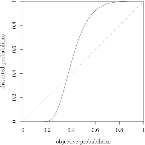
The difference between objective and distorted short-run risk is that short-run probabilities are now allowed to be distorted using a probability weighting function, in this case the one-parameter weighting function (2) proposed by Prelec (1998), which yields the highest likelihood. The parameter ψ in the Prelec function is estimated to be 3.74 and is significantly different from unity, since the absolute value of its t-value lies between 1.96 and 4.00; in fact $\left|t\right|=2.91$.

As shown in Figure 3, the estimated probability weighting function has an S-shaped pattern where small probabilities are underweighted and large probabilities are overweighted, which is in contrast to the inverse S-shaped probability weighting function often found in experiments. This contrast may be explained by the fact that with a positive background intensity of earthquakes, temporary deviations of short-run earthquake probabilities caused by seismic excitation are not evaluated (and overweighted) with respect to a reference probability of zero but with respect to a positive reference probability level. This applies in particular to Tokyo where the 90-day probability of an earthquake exceeding the magnitude threshold of 5.5 never drops below 35% in the period that we analyze.

Fig. 3 Estimated probability weighting of short-run probabilities, Prelec probability weighting function, $\widehat{\psi }=3.74$.

In summary: long-run risk matters, objective short-run risk does not, but distorted short-run risk does. In addition, all nonrisk parameter estimates in the second and third columns are similar to the ones in the first column and all are significant (with a t-value larger than 4.00 in absolute value).

We briefly comment on these other (nonrisk) parameters in the base model:

Intercept and city dummies

Tokyo, of course, is the most expensive city to buy property. If we set the property price level of Tokyo at 1.00, then the average property price levels of the other cities are 0.77 in Osaka, 0.66 in Nagoya, 0.40 in Fukuoka, and 0.29 in Sapporo. (Recall that we do not regress price but log-price on these dummies.) Also, if we set the price of land and building at 1.00, then the average price of the other types of property are 0.85 for land only and 0.52 for condos.

Ward attractiveness

As discussed in Section 3, we selected 11 characteristics for each ward, divided into 6 categories. Only four of these 11 characteristics appear in our base model: percentage of immigrants (representing population); number of criminal offenses (representing safety); and unemployment ratio and percentage of executives (representing employment). Executives make a ward more attractive, while crime and unemployment make it less attractive. Immigrants too make a ward more attractive, which makes sense if we realize that the word “immigrant” refers to somebody moving into the ward from another municipality, usually within Japan. Hence, the more people move in from other areas in Japan, the more attractive the ward apparently is.

Economic indicators

Property prices are affected by general economic conditions, and two indicators appear in Table 3 and in our base model: $\text{log}\hspace{0.17em}(\text{GDP})$ and $\text{log}\hspace{0.17em}(\text{CPI})$, both of which have a positive effect on property prices. The inclusion of $\text{log}\hspace{0.17em}(\text{CPI})$ has the additional advantage that if we wish to explain real (rather than nominal) property prices, then all results remain the same except that the effect of $\text{log}\hspace{0.17em}(\text{CPI})$ is now 0.503 rather than 1.503. Hence, CPI has a positive effect not only on nominal but also on real property prices.

Property characteristics

A large (floor) area and proximity to the nearest station contribute positively to the price. New buildings are preferred to old ones, where we have included two dummies because major changes occurred in the regulations on earthquake-resistance standards in both 1981 and 2000. As a result, buyers prefer a house built between 1981 and 2000 over a house built before 1981, and they like a house built after 2000 even better. Regarding the structure, wood is not desirable, steel is desirable, but reinforced concrete is preferred. Urban control signifies restrictions on development possibilities, and this has a negative effect on prices.

For all three property types, the designated maximum BCR and the maximum FAR are provided. These ratios are legally allowed maxima, different for each piece of land. The BCR is the percentage of the building area to the site area; the FAR is the percentage of the total floor area to the site area. We use both ratios in our regression and find a negative effect of BCR and a positive effect of FAR. Shimizu and Nishimura (2006) and Nakagawa, Saito, and Yamaga (2009) used only FAR and found mixed effects and a positive effect, respectively. Hidano, Hoshino, and Sugiura (2015) used both ratios (as we do) and found a negative effect of BCR and a mixed effect of FAR.

Quarterly effects

Estate agents sometimes tell customers that some months are better to buy or sell than others. Our results (in quarters, not months) are ambiguous, which is why we have omitted the quarter dummies from our regression. We return to this issue in our sensitivity analysis, see Appendix B (supplementary material).

Error components

We estimated the coefficients using the multivariate three-error components structure, as described in Section 5. It turns out that$$\text{tr}({\Sigma }_{ϵ})=0.406>\text{tr}({\Sigma }_{\zeta })=0.129\gg \text{tr}({\Sigma }_{\eta })=0.002,$$and as a result we set ${\Sigma }_{\eta }=0$, so that we end up with a two-error components structure. The effect of this is negligible and will be discussed further in our sensitivity analysis in Appendix B (supplementary material).

Appendix C (supplementary material) provides a detailed analysis of the corresponding impact of each of the explanatory variables component on the (log) property prices, and the premia for earthquake risk embedded in property prices. We find in particular that the joint impact of long-run and distorted short-run earthquake risk amounts to an average –2.0% of log property prices, which translates in monetary terms into a marginal effect of around –7 million Japanese yen per property—slightly more than the average annual income of a middle-income Japanese household in the period 2006/Q2 to 2015/Q3 we analyze. The impacts of long-run and distorted short-run earthquake risk are nearly the same for all property types but differ substantially among cities. Furthermore, the earthquake risk variables stand almost on equal footing with ward characteristics in explaining dispersion in property prices.

7 An Extension

In our base model, we use objective long-run probabilities and distorted short-run probabilities based on the Prelec probability weighting function. This raises various questions. First, one could argue that we should allow long-run probabilities to be distorted too; and second, we could experiment with different probability weighting functions.

In Table 4, we experiment with an alternative functional form for the short-run risk variable, namely the weighting function (1) introduced by Tversky and Kahneman (1992). In particular, in column 2 (Dist. SR, TK) we replace the Prelec function applied to the short-run earthquake probabilities with the Tversky-Kahneman probability weighting function. The estimation results are similar to the base model, but somewhat less precise, and the loglikelihood decreases. The Tversky-Kahneman probability weighting function is found to be S-shaped, just like the Prelec function, confirming the robustness of this finding.

Table 4 Sensitivity and extension—probability weighting functions.

	Base	Dist. SR	Dist. LR	Dist. LR
		TK	Prelec	TK
Area (m${}^2$)	0.0025	0.0025	0.0025	0.0025
Floor area (m${}^2$)	0.0006	0.0006	0.0006	0.0006
Distance to nearest station	−0.0145	−0.0145	−0.0143	−0.0143
Age	−0.0121	−0.0121	−0.0121	−0.0121
Long run 45–55	−0.1427	−0.1427	−0.8644	−0.4856
Long run 55+	−0.5041	−0.5039	−1.3838	−1.5028
Short run	−0.0514	−0.0733${}^{‡}$	−0.0517	−0.0518
$\widehat{\psi }$	3.74${}^{†}$	1.40${}^{‡}$	3.78${}^{†}$	3.77${}^{†}$
$\widehat{\gamma }$	–	–	0.17	0.32
$\Delta \hspace{0.17em}\text{log}\hspace{0.17em}L$	–	−14.6	152.8	167.6

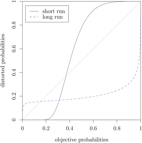
Next, we also allow long-run risk to be distorted using both the Prelec and the Tversky-Kahneman weighting functions. The model contains two related time-invariant long-run probabilities and we quite naturally assume that these two probabilities share the same weighting function with the same parameter γ. (In particular, distorted long run 45–55 is computed as distorted long run 45+ minus distorted long run 55+, consistent with Choquet integration.) In columns 3 and 4 of Table 4 we allow both long-run risk and short-run risk to be distorted.

The model with the higher likelihood is the one with an inverse S-shaped Tversky-Kahneman weighting function for long-run risk and an S-shaped Prelec weighting function for short-run risk, as shown in Figure 4. We note that the Prelec function for long-run risk, although yielding a lower loglikelihood than the Tversky-Kahneman weighting function, is also found to be inverse S-shaped, which is again reassuring for the robustness of our results. Thus, in an extension of our base model that allows for distortion of time-invariant long-run earthquake probabilities we find evidence of a conventional inverse S-shaped probability weighting function for long-run earthquake probabilities. This means that when purchasing property in Japan, people tend to overweight small long-run probabilities and underweight large long-run probabilities.

Fig. 4 Implied probability weighting functions of long-run and short-run earthquake risk.

8 Conclusion

We have studied the impact of earthquake risk on Japanese property prices using a rich panel dataset. We have not only allowed for time-invariant long-run earthquake probabilities to impact property prices, but we have also analyzed the impact of short-run earthquake probabilities generated from a seismic excitation model. We have designed a hedonic property prices model that accommodates probability weighting, employing a multivariate error components structure, and have developed the associated maximum likelihood and variance computation procedures. We have shown that long-run earthquake probabilities negatively impact property prices and increasingly so at higher risk levels. We have also shown that short-run earthquake probabilities have a negative impact on property prices, and that this effect becomes statistically significant only after we allow for probability weighting.

The probability weighting function associated with short-run earthquake probabilities is found to be S-shaped. That stands in contrast to the familiar inverse S-shaped probability weighting functions predominantly found in experiments. The shape we find may be explained by the fact that in our setting there is a nonnegligible positive background arrival rate of earthquakes. People may therefore tend to evaluate earthquake probabilities, and overweight their temporary deviations under seismic excitation, not with respect to zero but with respect to a positive reference probability level. This remarkable finding calls for the development of reference-dependent models for probabilities to augment the large literature on reference-dependent models for changes in wealth levels.

Our objective short-run earthquake probabilities are based on a purely temporal ETAS model. Within the spatial windows used for estimation of the ETAS model, it is assumed that the earthquake intensity functions, and people’s perception of seismic risk, are homogeneous (see also our Data Documentation). A refinement that accounts for spatial variation would be desirable, but is subject to statistical and computational complications. Addressing the potential limitations inherent in using a purely temporal ETAS model in this context is an interesting and challenging problem for future research.

Acknowledgments

We are very grateful to the editor, associate editor and three referees for thoughtful comments and suggestions that have significantly improved the article. Earlier versions of this article were presented at Keio University in Tokyo, the Technische Universität Wien, the Universities of Oxford, Madrid and Fudan, and at the 2018 Econometric Society Australasian Meeting in Auckland and the 2018 China Meeting of the Econometric Society in Shanghai. We thank the participants and in particular Yoshitsugu Kanemoto for helpful comments.

Supplementary Material

This article comes with three supplementary files. First, the Appendix which contains various technical results, a discussion of the robustness of our estimation results, an analysis of the influence of each component to the total property prices and the implied premia for earthquake risk, a brief literature review, and an auxiliary figure. Second, the Data Documentation, which contains a detailed description of the data, and is available from https://bit.ly/3qHcTQ3. And third, the cleaned and compiled datasets and all codes to implement the procedures developed in this article, including our multivariate error components regression R package mvecr, available from https://github.com/yy112/earthquake-risk.

Additional information

Funding

This research was supported in part by the Japan Society for the Promotion of Science (JSPS) under grant 16K03565 (Ikefuji) and the Netherlands Organization for Scientific Research (NWO) under grant VIDI (Laeven).

Notes

¹ The Data Documentation is available from https://bit.ly/3qHcTQ3.

² Data and codes are available from https://github.com/yy112/earthquake-risk.

³ The multivariate error components regression R package mvecr that we have developed for this article is available from the article’s github page.

References

- Abdellaoui, M. (2000), “Parameter-Free Elicitation of Utility and Probability Weighting Functions,” Management Science, 46, 1497–1512. DOI: https://doi.org/10.1287/mnsc.46.11.1497.12080.
- Aït-Sahalia, Y., Laeven, R. J. A., and Pelizzon, L. (2014), “Mutual Excitation in Eurozone Sovereign CDS,” Journal of Econometrics, 183, 151–167. DOI: https://doi.org/10.1016/j.jeconom.2014.05.006.
- Aït-Sahalia, Y., Cacho-Diaz, J. A., and Laeven, R. J. A. (2015), “Modeling Financial Contagion Using Mutually Exciting Jump Processes,” Journal of Financial Economics, 117, 585–606. DOI: https://doi.org/10.1016/j.jfineco.2015.03.002.
- Avery, R. B. (1977), “Error Components and Seemingly Unrelated Regressions,” Econometrica, 45, 199–209. DOI: https://doi.org/10.2307/1913296.
- Baltagi, B. H. (1980), “On Seemingly Unrelated Regressions with Error Components,” Econometrica, 48, 1547–1551. DOI: https://doi.org/10.2307/1912824.
- Baltagi, B. H. (2008), Econometric Analysis of Panel Data, New York: Wiley.
- Beron, K. J., Murdoch, J. C., Thayer, M. A., and Vijverberg, W. P. M. (1997), “An Analysis of the Housing Market Before and After the 1989 Loma Prieta Earthquake,” Land Economics, 73, 101–113. DOI: https://doi.org/10.2307/3147080.
- Bin, O., and Landry, C. E. (2013), “Changes in Implicit Flood Risk Premiums: Empirical Evidence From the Housing Market,” Journal of Environmental Economics and Management, 65, 361–376. DOI: https://doi.org/10.1016/j.jeem.2012.12.002.
- Bin, O., and Polasky, S. (2004), “Effects of Flood Hazards on Property Values: Evidence Before and After Hurricane Floyd,” Land Economics, 80, 490–500. DOI: https://doi.org/10.2307/3655805.
- Boswijk, H. P., Laeven, R. J. A., and Lalu, A. (2016), “Asset Returns with Self-Exciting Jumps: Option Pricing and Estimation with a Continuum of Moments,” Mimeo, University of Amsterdam.
- Brookshire, D. S., Thayer, M. A., Tschirhart, J., and Schulze, W. D. (1985), “A Test of the Expected Utility Model: Evidence From Earthquake Risks,” Journal of Political Economy, 93, 369–389. DOI: https://doi.org/10.1086/261304.
- Chamberlain, G., and Griliches, Z. (1975), “Unobservables with a Variance-Components Structure: Ability, Schooling, and the Economic Success of Brothers,” International Economic Review, 16, 422–449. DOI: https://doi.org/10.2307/2525824.
- Daniel, V. E., Florax, R. J. G. M., and Rietveld, P. (2009), “Flooding Risk and Housing Values: An Economic Assessment of Environmental Hazard,” Ecological Economics, 69, 355–365. DOI: https://doi.org/10.1016/j.ecolecon.2009.08.018.
- Demidenko, E. (2013), Mixed Models: Theory and Application with R (2nd ed.), New York: Wiley.
- Dutta, S., and Mondal, D. (2015), “An h-Likelihood Method for Spatial Mixed Linear Models Based on Intrinsic Auto-Regressions,” Journal of the Royal Statistical Society, Series B, 77, 699–726. DOI: https://doi.org/10.1111/rssb.12084.
- Dutta, S., and Mondal, D. (2016), “REML Estimation with Intrinsic Matérn Dependence in the Spatial Linear Mixed Model,” Electronic Journal of Statistics, 10, 2856–2893.
- Eeckhoudt, L. R., Laeven, R. J., and Schlesinger, H. (2020), “Risk Apportionment: The Dual Story,”Journal of Economic Theory, 185, 104971. DOI: https://doi.org/10.1016/j.jet.2019.104971.
- Gu, T., Nakagawa, M., Saito, M., and Yamaga, H. (2011), “On Asymmetric Effects of Changes in Regional Risk Rankings on Relative Land Prices in the Tokyo Metropolitan Area: A Test of Implications Implied by Prospect Theory Using Market Equilibrium Prices (in Japanese),” Journal of Behavioral Economics and Finance, 4, 1–19.
- Hanaoka, C., Shigeoka, H., and Watanabe, Y. (2018), “Do Risk Preferences Change? Evidence From the Great East Japan Earthquake,” American Economic Journal: Applied Economics, 10, 298–330. DOI: https://doi.org/10.1257/app.20170048.
- Heckerman, D., Gurdasani, D., Kadie, C., Pomilla, C., Carstensen, T., Martin, H., Ekoru, K., Nsubuga, R. N., Ssenyomo, G., Kamali, A., Kaleebu, P., Widmer, C., and Sandhu, M. S. (2016), “Linear Mixed Model for Heritability Estimation that Explicitly Addresses Environmental Variation,” Proceedings of the National Academy of Sciences, 113, 7377–7382. DOI: https://doi.org/10.1073/pnas.1510497113.
- Hidano, N., Hoshino, T., and Sugiura, A. (2015), “The Effect of Seismic Hazard Risk Information on Property Prices: Evidence From a Spatial Regression Discontinuity Design,” Regional Science and Urban Economics, 53, 113–122. DOI: https://doi.org/10.1016/j.regsciurbeco.2015.05.005.
- Jiang, J., Rao, J. S., Gu, Z., and Nguyen, T. (2008), “Fence Methods for Mixed Model Selection,” Annals of Statistics, 36, 1669–1692.
- Jiang, J., and Nguyen, T. (2015), The Fence Methods, Singapore: World Scientific.
- Kahneman, D., and Tversky, A. (1979), “Prospect Theory: An Analysis of Decision Under Risk,” Econometrica, 47, 263–292. DOI: https://doi.org/10.2307/1914185.
- Kawawaki, Y., and Ota, M. (1996), “The Influence of the Great Hanshin-Awaji Earthquake on the Local Housing Market,” Review of Urban and Regional Development Studies, 8, 220–233. DOI: https://doi.org/10.1111/j.1467-940X.1996.tb00119.x.
- Lippert, C., Listgarten, J., Liu, Y., Kadie, C. M., Davidson, R. I., and Heckerman, D. (2011), “FAST Linear Mixed Models for Genome-Wide Association Studies,” Nature Methods, 8, 833–835. DOI: https://doi.org/10.1038/nmeth.1681.
- Magnus, J. R. (1982), “Multivariate Error Components Analysis of Linear and Nonlinear Regression Models by Maximum Likelihood,” Journal of Econometrics, 19, 239–285. DOI: https://doi.org/10.1016/0304-4076(82)90005-7.
- Nakagawa, M., Saito, M., and Yamaga, H. (2007), “Earthquake Risk and Housing Rents: Evidence From the Tokyo Metropolitan Area,” Regional Science and Urban Economics, 37, 87–99. DOI: https://doi.org/10.1016/j.regsciurbeco.2006.06.009.
- Nakagawa, M., Saito, M., and Yamaga, H. (2009), “Earthquake Risks and Land Prices: Evidence From the Tokyo Metropolitan Area,” The Japanese Economic Review, 60, 208–222.
- Naoi, M., Seko, M., and Ishino, T. (2012), “Earthquake Risk in Japan: Consumers’ Risk Mitigation Responses After the Great East Japan Earthquake,” Journal of Economic Issues, 46, 519–529. DOI: https://doi.org/10.2753/JEI0021-3624460227.
- Naoi, M., Seko, M., and Sumita, K. (2009), “Earthquake Risk and Housing Prices in Japan: Evidence Before and After Massive Earthquakes,” Regional Science and Urban Economics, 39, 658–669. DOI: https://doi.org/10.1016/j.regsciurbeco.2009.08.002.
- Ogata, Y. (1981), “On Lewis’ Simulation Method for Point Processes,” IEEE Transactions on Information Theory, 27, 23–31. DOI: https://doi.org/10.1109/TIT.1981.1056305.
- Ogata, Y. (1988), “Statistical Models for Earthquake Occurrences and Residual Analysis for Point Processes,” Journal of the American Statistical Association, 83, 9–27.
- Prelec, D. (1998), “The Probability Weighting Function,” Econometrica, 66, 497–527. DOI: https://doi.org/10.2307/2998573.
- Quiggin, J. (1982), “A Theory of Anticipated Utility,” Journal of Economic Behavior and Organization, 3, 323–343. DOI: https://doi.org/10.1016/0167-2681(82)90008-7.
- Rosen, S. (1974), “Hedonic Prices and Implicit Markets: Product Differentiation in Pure Competition,” Journal of Political Economy, 82, 34– 55. DOI: https://doi.org/10.1086/260169.
- Shimizu, C., and Nishimura, K. G. (2006), “Biases in Appraisal Land Price Information: The Case of Japan,” Journal of Property Investment and Finance, 24, 150–175. DOI: https://doi.org/10.1108/14635780610655102.
- Tversky, A., and Kahneman, D. (1992), “Advances in Prospect Theory: Cumulative Representation of Uncertainty,” Journal of Risk and Uncertainty, 5, 297–323. DOI: https://doi.org/10.1007/BF00122574.
- Von Neumann, J., and Morgenstern, O. (1944), Theory of Games and Economic Behavior (3rd ed.), Princeton, NJ: Princeton University Press.
- Wakker, P. P. (2008), “Explaining the Characteristics of the Power (CRRA) Utility Family,” Health Economics, 17, 1329–1344. DOI: https://doi.org/10.1002/hec.1331.
- Wu, G., and Gonzalez, R. (1996), “Curvature of the Probability Weighting Function,” Management Science, 42, 1676–1690. DOI: https://doi.org/10.1287/mnsc.42.12.1676.
- Yaari, M. E. (1987), “The Dual Theory of Choice Under Risk,” Econometrica, 55, 95–115. DOI: https://doi.org/10.2307/1911158.
- Yamaga, H., Nakagawa, H., and Saito, M. (2002), “Earthquake Risks and Land Pricing: The Case of the Tokyo Metropolitan Area (in Japanese),” Journal of Applied Regional Science, 7, 51–62.