Modeling Pregnancy Outcomes Through Sequentially Nested Regression Models

Abstract

The polycystic ovary syndrome (PCOS) is a most common cause of infertility among women of reproductive age. Unfortunately, the etiology of PCOS is poorly understood. Large-scale clinical trials for pregnancy in polycystic ovary syndrome (PPCOS) were conducted to evaluate the effectiveness of treatments. Ovulation, pregnancy, and live birth are three sequentially nested binary outcomes, typically analyzed separately. However, the separate models may lose power in detecting the treatment effects and influential variables for live birth, due to decreased sample sizes and unbalanced event counts. It has been a long-held hypothesis among the clinicians that some of the important variables for early pregnancy outcomes may continue their influence on live birth. To consider this possibility, we develop an ${\mathcal{l}}_0$-norm based regularization method in favor of variables that have been identified from an earlier stage. Our approach explicitly bridges the connections across nested outcomes through computationally easy algorithms and enjoys theoretical guarantee of estimation and variable selection. By analyzing the PPCOS data, we successfully uncover the hidden influence of risk factors on live birth, which confirm clinical experience. Moreover, we provide novel infertility treatment recommendations (e.g., letrozole vs. clomiphene citrate) for women with PCOS to improve their chances of live birth. Supplementary materials for this article are available online.

Keywords:

• Infertility study
• ${\mathcal{l}}_0$ penalization
• Sequentially nested binary outcome
• Variable selection

1 Introduction

The polycystic ovary syndrome (PCOS), characterized by metabolic abnormalities, is the most common cause of infertility affecting up to 10% of reproductive-age women (Azziz et al. 2004). This gynecological condition leads to health consequences such as anovulation and early pregnancy loss, with other common manifestations including obesity and type 2 diabetes (Legro et al. 2007). Despite its high prevalence and importance of public health, unfortunately, the etiology of PCOS remains obscure, and both the diagnosis and treatment of this disorder are surrounded by controversy. There are many challenges in studying and treating PCOS; for example, the following are two challenges that need to be addressed. The first challenge stems from the lacking of evidence-based recommendations for infertility treatment; hence, physicians have always struggled to recommend first-line therapy to restore ovulation due to the divergent conclusions reached by studies (Legro et al. 2007). The second challenge is to understand heterogeneity of PCOS and plan personalized infertility treatment, which is still open to discussion since women with PCOS are phenotypically diverse (Rausch et al. 2009).

Our investigation is motivated by and applied to the pregnancy in polycystic ovary syndrome (PPCOS) trials, which were double-blinded, multi-center, randomized clinical trials (Legro et al. 2007, 2014) completed by the Reproductive Medicine Network. The goal was to evaluate and recommend the optimal ovulation induction regimen. Live birth was the primary outcome for both trials following a broad consensus of infertility studies (Legro and Myers 2004; Harbin Consensus Conference Workshop Group 2014). Secondary outcomes included ovulation and clinical pregnancy that were milestones preceding a possible live birth delivery. In the first trial, referred to as PPCOS I, 626 infertile women, aged 18–39 years, were enrolled between November 2002 and December 2004. The second trial, called PPCOS II, enrolled 750 infertile women, aged 18–40 years, between February 2009 and January 2012. All the participants were diagnosed with PCOS according to symptoms such as anovulation, polycystic ovaries, and hyperandrogenism (ESHRE, The Rotterdam and ASRM-Sponsored PCOS Consensus Workshop Group 2004). Each participant of the study was randomly assigned to one of the treatment arms. The PPCOS I was the largest published study examining the efficacy of clomiphene citrate, metformin and the combination of the two among women with PCOS (Legro et al. 2007). The PPCOS II compared letrozole to clomiphene citrate for infertility treatment among women with PCOS (Legro et al. 2014).

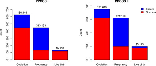
To tackle the aforementioned challenges and further our understanding of PCOS, in this study we aim to identify treatments and easily obtainable baseline measures that may improve ovulation, pregnancy, and ultimately live birth rates, which would be beneficial in counseling patients regarding their prognosis and therapy. Figure 1 visualizes the data structure of the outcomes in the PPCOS I and II trials.

Fig. 1 Summary of outcomes in the PPCOS study, with total of 626 and 750 participants in the PPCOS I and PPCOS II, respectively. The ratios of failure and success are presented over the bars.

A distinct feature of the pregnancy outcomes is the sequentially nested binary outcomes (SNBOs). The subsequent success is conditional upon the preceding one. SNBOs are common in many biomedical research. A natural strategy to model SNBOs is through the sequential logistic regression (Tutz 1991), which is also referred to by a variety of other names including sequential response model (Maddala 1986), model for nested dichotomies (Fox 1997), and continuation ratio logit model (Agresti 2002). In a sequential logistic regression, each of the outcomes is modeled separately with the observations whose preceding outcome is a “success.” For example, we may model the outcome “pregnancy” by using the observations from the women who ovulated, and likewise model the outcome “live birth” by using the observations from the pregnant women only. Therefore, a sequential logistic regression can be estimated easily by considering one response at a time and estimating a sequence of logistic regressions. Indeed, this strategy is widely adopted by clinical practitioners, see, for example, Chen et al. (2016) and Wu et al. (2017).

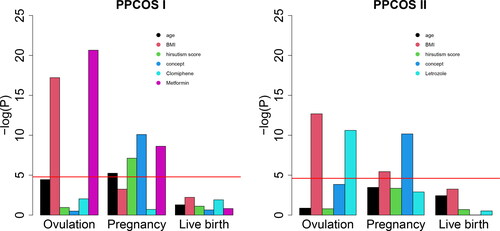
However, as the sequential logistic regression models each outcome separately, it does not leverage all the potentially useful information from precedent outcomes and can lose power to detect the influential variables. This limitation becomes more severe for the later stage outcomes due to the smaller sample sizes and unbalanced event counts. For example, among the 133 women in the PPCOS I who achieved pregnancy, 118 of them delivered live birth, while 15 of them did not, causing the imbalance between the two event counts. In practice, clinicians usually perform a sequential logistic regression with the covariates determined by clinical knowledge and/or variable screening. Often, however, very few covariates are significantly associated with live birth (Kuang et al. 2015; Hansen et al. 2016). Regardless of the significance, roles of some covariates are often assumed a priori and these covariates are kept in the final regression model anyway. This may not be able to advance our understanding of PCOS and even provide misleading information. As a proof of principle, we included the treatments and four variables that were supposedly clinically relevant in a sequential logistic regression for the PPCOS data, none of the predictors were statistically significant for live birth when the p-value was set at 0.05 and adjusted by the Bonferroni correction; see Figure 2. This observation discourages further and potentially useful investigation.

Fig. 2 P-values of the sequential logistic regression for the PPCOS data. The red lines indicate the nominal significance level 0.05 adjusted by the Bonferroni correction.

To leverage the unique structure of SNBOs, it is desirable to develop approaches that analyze the outcomes jointly and allow the model to borrow the information of variable selection from precedent outcomes. Although the influential variables for each outcome may be different, it is reasonable to expect that the identified variables for the early pregnancy outcomes are more likely to influence the later pregnancy outcomes. Therefore, a sensible strategy is to give preference to variables that have been identified from an earlier stage. This is the key idea behind our method that has never been investigated before.

Building from the sequential logistic regression models, we develop an ${\mathcal{l}}_0$-norm based regularization method in favor of variables that have been identified for the earlier stage outcomes. Our approach explicitly bridges the connections across nested outcomes through computationally easy algorithms and enjoys oracle properties on estimation and variable selection under usual regularity conditions. Numerical results demonstrate that our proposed method clearly outperforms the existing methods that model the outcomes separately. The proposed method is beneficial regardless of whether the true influential variables for multiple outcomes are overlapping and whether the number of explanatory variables is smaller than the sample size. By applying our method to the PPCOS data, we are able to recommend infertility treatment strategies for women with PCOS to improve their chances of live birth.

The rest of this paper is organized as follows. In Section 2, we introduce our method including likelihood function and regularization. Section 3 describes the computational algorithms. We present the theoretical properties in Section 4. In Section 5, we conduct a comprehensive simulation study. The results of analyzing the PPCOS data are presented in Section 6. We conclude with some remarks in Section 7. Supplementary materials containing technical details and extra results for numerical studies are available online.

2 Methods

2.1 Modeling Framework

Consider a dataset with n subjects, where each subject has M SNBOs and p explanatory variables. For the ith subject ($i=1,\dots ,n$), let ${\mathbf{y}}_{i,·}={(y_{i,1},\dots ,y_{i,M})}^{\top }\in {\{0,1\}}^M$ denote the M-dimension binary outcome with nested structure. The binary outcomes are nested in the sense that $y_{i,m}$ can be observed if and only if the precedent outcome $y_{i,m-1}=1$. That is to say, $y_{i,m-1}=0$ is an absorbing stage that no further outcome is available. In the infertility study, M = 3 and the three outcomes correspond to ovulation, pregnancy and live birth. Furthermore, let ${\mathbf{X}}_{i,·}=(X_{i,1},\dots ,X_{i,p})$ be a p-dimensional row vector of the explanatory variables for subject i. We allow a high-dimensional setting that the number of explanatory variables p is not necessarily less than the sample size n. The aim is to develop a statistical model to accommodate SNBOs and select influential variables for M outcomes both individually and jointly.

Let $y_{i,0}=1$ for $i=1,\dots ,n$, a natural way to formulate the dataset is through a sequence of generalized linear models:(1) $$g\left(\mathbb{E}(y_{i,m}|y_{i,m-1}=1,{\mathbf{X}}_{i,·})\right)={\mathbf{X}}_{i,·}{\beta }_{·,m}+{\alpha }_m,m=1,\dots ,M,$$(1) where $g(·)$ is certain link function, α_m and ${\beta }_{·,m}={({\beta }_{1,m},\dots ,{\beta }_{p,m})}^{\top }$ are the unknown intercept and coefficients for outcome m. As we are considering binary responses, commonly used link functions $g(·)$ include the logit link $g(\pi )=\hspace{0.17em}\text{log}\hspace{0.17em}(\pi /(1-\pi ))$ and probit link $g(\pi )={\Phi }^{-1}(\pi )$. Although we can use either the logit or probit link function in our method, we restrict our attention to the logit link from now on. Model (1) is the typical setting of a sequential logistic regression model. It may be viewed as the most natural model for SNBOs in the sense that it only assumes a conditional mean structure given the precedent outcome is “success.”

We let $\beta =({\beta }_{·,1},\dots ,{\beta }_{·,M})\in {\mathbb{R}}^{p\times M}$ be the coefficients matrix. Let ${\beta }_{j,·}=({\beta }_{j,1},\dots ,{\beta }_{j,M})$ be the jth row of the coefficients matrix, so $\beta =({\beta }_{·,1},\dots ,{\beta }_{·,M})={({\beta }_{1,·}^{\top },\dots ,{\beta }_{p,·}^{\top })}^{\top }$. Let $\alpha =({\alpha }_1,\dots ,{\alpha }_M)$. Let ${\mathbf{y}}_{·,m}={(y_{1,m},\dots ,y_{n,m})}^{\top }$ denote the m-th stage response vector, so $\mathbf{Y}=({\mathbf{y}}_{·,1},\dots ,{\mathbf{y}}_{·,M})={({\mathbf{y}}_{1,·}^{\top },\dots ,{\mathbf{y}}_{n,·}^{\top })}^{\top }$. In addition, let ${\Omega }_1=\{1,\dots ,n\}$ and ${\Omega }_m=\{i\in 1,\dots ,n,y_{i,m-1}=1\},m=2,\dots ,M$, denote the set of observations that $y_{i,m}$ is available. Then we have ${\Omega }_M\subseteq {\Omega }_{M-1}\subseteq \dots \subseteq {\Omega }_1=\{1,\dots ,n\}$. We further let $n_m=\left|{\Omega }_m\right|$ be the number of available observations for outcome ${\mathbf{y}}_{·,m}$. Furthermore, denote the design matrix $\mathbf{X}={({\mathbf{X}}_{1,·}^{\top },\dots ,{\mathbf{X}}_{n,·}^{\top })}^{\top }=({\mathbf{X}}_{·,1},\dots ,{\mathbf{X}}_{·,p})$. With a little abuse of notation, let ${\mathbf{X}}_m={({\mathbf{X}}_{i,·}^{\top },i\in {\Omega }_m)}^{\top }$ denote the sub matrix of $\mathbf{X}$ with the observation in Ω _m and ${\mathbf{X}}_{m,j}$ denote jth column of ${\mathbf{X}}_m$. Finally, assume without loss of generality that $\mathbf{X}$ is normalized such that $\left|\right|{\mathbf{X}}_{·,j}|{|}_2^2=n$.

2.2 Likelihood Function

As variable selection is desired in our study, penalization methods are adopted. Let $\mathcal{l}(\beta )$ be the negative likelihood function of the nested outcomes, $\text{Pen}(\beta )$ be the penalty function. We aim to minimize the penalized negative log-likelihood function$$L(\beta )=\mathcal{l}(\beta )+\text{Pen}(\beta ).$$

We will specify the forms of $\mathcal{l}(\beta )$ and $\text{Pen}(\beta )$ in this and next subsections, respectively.

Given an observed response $\mathbf{Y}$ and covariates matrix $\mathbf{X}$, the conditional probability of $\mathbf{Y}$ given $\mathbf{X}$ under the sequential logistic model (1) is(2) $$\mathbb{P}(\mathbf{Y}|\mathbf{X})=\prod _{m=1}^M\prod _{i\in {\Omega }_m}{({\pi }_{i,m})}^{y_{i,m}}{(1-{\pi }_{i,m})}^{1-y_{i,m}},$$(2) where ${\pi }_{i,m}=\mathbb{E}(y_{i,m}|y_{i,m-1}=1,{\mathbf{X}}_{i,·})=h({\mathbf{X}}_{i,·}^{\top }{\beta }_{·,m}+{\alpha }_m)$ and $h(x)=\hspace{0.17em}\text{exp}\hspace{0.17em}(x)/(1+\hspace{0.17em}\text{exp}\hspace{0.17em}(x))$. The negative log-likelihood then equals(3) $$\mathcal{l}(\beta )=-\frac{1}{n}\text{log}\hspace{0.17em}\mathbb{P}(\mathbf{Y}|\mathbf{X})=\sum _{m=1}^M{\mathcal{l}}^m({\beta }_{·,m}),$$(3) (4) $$\begin{array}{c}{\mathcal{l}}^m({\beta }_{·,m})=-\frac{1}{n}\sum _{i\in {\Omega }_m}\{y_{i,m}({\mathbf{X}}_{i,·}^{\top }{\beta }_{·,m}+{\alpha }_m)\\ +\hspace{0.17em}\text{log}\hspace{0.17em}(1+\hspace{0.17em}\text{exp}\hspace{0.17em}({\mathbf{X}}_{i,·}^{\top }{\beta }_{·,m}+{\alpha }_m))\}.\end{array}$$(4)

By (3), we see that the maximum likelihood estimator (MLE) of $\mathcal{l}(·)$ is a matrix whose columns are the MLEs of ${\mathcal{l}}^m(·)$. This validates the statement that sequential logistic model can be estimated easily by estimating a sequence of logistic models.

2.3 Penalty Function

In this section, we develop a novel penalization method to leverage the unique structure of SNBOs. The penalty function $\text{Pen}(\beta )$ is mixed with two parts as follows.

In the first part of $\text{Pen}(\beta )$, we use an ${\mathcal{l}}_1$ penalization Lasso (Tibshirani 1996) to account for a general sparse structure of the regression coefficients for all the outcomes. As one of the most popular penalty functions, Lasso is easy to compute and naturally provides a sparse solution for variable selection. In our analysis, we penalize the coefficients ${\beta }_{·,m}$ in each stage with the absolute penalty and combine them together: ${\lambda }_1{\sum }_{m=1}^M\left|\right|{\beta }_{·,m}|{|}_1$. Here ${\lambda }_1\ge 0$ is the common penalty level for the coefficients in each of the stages $m=1,\dots ,M$. Theoretically, the penalty levels at different stages should be different, as an oracle penalty level should depend on the sample size of different outcomes. But in our analysis, a mixture of two penalty functions is applied. The second part of the penalty would leverage the difference between outcomes. Therefore, to reduce the computational burden of tuning too many parameters, a common penalty level is adopted in the above penalty.

The second part of $\text{Pen}(\beta )$ aims to leverage the unique structure of SNBOs. As discussed in Section 1, it is a common sense that important factors may have lasting influence: the identified variables for the early pregnancy outcomes are more likely to influence the later pregnancy outcomes. In other words, we penalize the coefficients that are identified at stage m – 1 but dropped at stage m for $m=2,\dots ,M$. 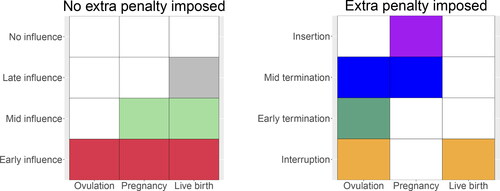To illustrate this idea further, Figure 3 displays all 8 scenarios for a variable to be selected or not with respect to the three SNBOs of the PPCOS data and which scenarios we wish to impose additional penalties. Overall, we encourage the continuous influence of covariates on live birth including early, mid, and late influence as shown in Figure 3.

Fig. 3 Possible scenarios for a variable to be selected (colored cells) or not (blank cells) with respect to the three outcomes. The left-hand side presents the four scenarios (no, late, mid, and early influence) when variables selected earlier are kept later. In this case, we do not wish to impose additional penalties on those selected variables. The right hand side presents the other four scenarios (insertion, mid and early termination, interruption) when some variables are selected at some point and dropped at another point later. This is the case that we impose additional penalties.

For a general M, if we write ${\beta }_{j,0}=0$ for $j=1,\dots ,p$, we employ the following penalty to carry out our intent(5) $${\lambda }_2\sum _{j=1}^p\sum _{m=1}^M\left\{\rho (|{\beta }_{j,m-1}|+a|{\beta }_{j,m}|)-\rho (|{\beta }_{j,m}|)\right\},$$(5) where $\rho (t)=I(t\ne 0)$ is the ${\mathcal{l}}_0$ penalty, ${\lambda }_2\ge 0$ is the penalty level and a is a positive constant whose role shall be discussed shortly.

For any a > 0, the penalty (5) is minimized if none of the selected variables are dropped in a future stage, and is maximized if every selected variable is eventually dropped in a future stage. For example, zero penalty is imposed on the four scenarios in the first panel of Figure 3, but the penalty is equal to λ ₂ for the four scenarios in the second panel. Therefore, the penalty (5) encourages the model to sequentially incorporate influential variables from ovulation to live birth, the endpoint of the study. The parameter λ ₂ controls how “strong” the connection between the stages is. When ${\lambda }_2=0$, the proposed method reduces to M separate generalized linear models with Lasso penalty. When ${\lambda }_2=\infty$, it forces that $\text{supp}({\beta }_{·,1})\subseteq \text{supp}({\beta }_{·,2})\subseteq \cdots \subseteq \text{supp}({\beta }_{·,M})$.

As the ${\mathcal{l}}_0$ penalty norm is difficult to optimize, we use the seamless-L ₀ (SELO) penalty (Dicker, Huang, and Lin 2013; Li, Wang, and Lin 2012) instead to mimic the properties of ${\mathcal{l}}_0$ penalty and yet is easier to compute. With a little abuse of notation, the SELO is defined as(6) $$\rho (t)=\rho (t;\tau )=\frac{1}{\hspace{0.17em}\text{log}\hspace{0.17em}(2)}\text{log}\hspace{0.17em}\left(\frac{\left|t\right|}{\left|t\right|+\tau }+1\right),$$(6) with τ being a small positive constant. The derivatives of a SELO penalty is$$\dot{\rho }(t;\tau )=\frac{1}{\hspace{0.17em}\text{log}\hspace{0.17em}(2)}\frac{\text{sgn}(t)\tau }{(|t|+\tau )(2t+\tau )}.$$

The SELO is computationally easier and possesses the same asymptotic properties as the ${\mathcal{l}}_0$ norm. Intuitively, concave penalties, such as SCAD and MCP, can be alternatives to ${\mathcal{l}}_0$ penalty. However, we choose SELO to substitute the ${\mathcal{l}}_0$-norm, as it provides better approximations of ${\mathcal{l}}_0$ and addresses directly on variable selection. On the other side, the concave penalties emphasize the magnitudes of the coefficients for the covariates, but in our setting, the magnitudes corresponding to different covariates may not be comparable, as they are applied to different outcomes. We note that others also used SELO to mimic the effects of ${\mathcal{l}}_0$ penalty on variable selection in different studies. For example, Huang et al. (2017) used this strategy in integrative analysis to encourage the similarities of sparsity patterns across different datasets.

To use the SELO penalty, we require the tuning parameter a in (5) to be slightly larger than 1. To explain the heuristics behind this requirement, consider the case that ${\beta }_{j,m-1}=0$ and ${\beta }_{j,m}\ne 0$. In this case, $\rho (|{\beta }_{j,m-1}|+a|{\beta }_{j,m}|)-\rho (|{\beta }_{j,m}|)>0$ when a > 1. This imposes an additional term of penalization which prevents the stage m from adding too many variables from stage m – 1. On the other hand, too large an a may prevent the possibility of adding new variables. In other words, a may be viewed as a parameter to control the magnitude or possibility of adding new variables from precedent stages. See Section 3.2 for details on tuning parameters a and τ.

Together, we propose to minimize the following penalized log-likelihood function(7) $$\begin{array}{c}L(\beta )=-\frac{1}{n}\sum _{m=1}^M\sum _{i\in {\Omega }_m}\{y_{i,m}({\mathbf{X}}_{i,·}^{\top }{\beta }_{·,m}+{\alpha }_m)\\ +\hspace{0.17em}\text{log}\hspace{0.17em}(1+\hspace{0.17em}\text{exp}\hspace{0.17em}({\mathbf{X}}_{i,·}^{\top }{\beta }_{·,m}+{\alpha }_m))\}\end{array}$$(7) (8) $$\begin{array}{c}+{\lambda }_1\sum _{m=1}^M\left|\right|{\beta }_{·,m}|{|}_1+{\lambda }_2\sum _{j=1}^p\sum _{m=1}^M\{\rho (|{\beta }_{j,m-1}|\\ +a\left|{\beta }_{j,m}\right|;\tau )-\rho (\left|{\beta }_{j,m}\right|;\tau )\}.\end{array}$$(8)

2.4 Connections With Integrative Analysis and Hierarchical Variable Selection

Our approach for SNBOs shares some similarities with those used in integrative analysis that pools together individual data from multiple datasets and leverage a larger sample. The integrative analysis is closely related to a much commonly used meta-analysis that may use either individual data or summary information from multiple datasets. For example, Huang et al. (2017) proposed to leverage the datasets connections by promoting the similarity in sparsity structure of coefficients in integrative analysis. In addition, Shi et al. (2014) accommodated the across-dataset structures by smoothing the magnitude of regression coefficients of same covariates.

On the other hand, our approach for SNBOs differs significantly from integrative analysis in the following key aspects. First, unlike the integrative analysis that pools information from multiple independent datasets, SNBOs are dealing with a same set covariates which has particular scientific or other implications that make it even more desirable to incorporate its unique structures in the analysis. Second, integrative analysis usually promotes the similarity of sparsity structures, which is not appropriated in SNBOs which have a nested structure.

In addition, it is also noteworthy to mention the differences between our approach and some existing variable selection approaches for dataset with special structures. For example, there are models that have a natural hierarchy, such as polynomial models, where higher order or interaction terms should only be included in the model after its corresponding main effects. Moreover, there are also models that have a natural grouping effect, where certain variables should be kept in or removed from the model simultaneously. To address the hierarchical or grouping structure, composite (Zhao, Rocha, and Yu 2009) or group (Yuan and Lin 2006) penalization methods have been proposed in the literature. Differing from these approaches, our method for SNBOs aims to address the connections across different outcomes with the same variable/term, while group/hierarchy structure is for the same outcome but different variable/term. Furthermore, our method is more flexible. The identified variables for early pregnancy outcomes are more likely, but not necessary, to have effects on the later pregnancy outcomes, but the group based Lasso approach imposes strict structures in that the variables in a group are either selected or not selected altogether.

3 Computation

In this section, we discuss the optimization algorithm for (7). This was achieved through a combination of iteratively reweighted least squares (IRLS) and a block coordinate descent (BCD) algorithm. The IRLS approximates the objective function (7) in the outer loop and the BCD computes the approximated objective function obtained by IRLS in the inner loop. Our procedure is similar to that in Friedman, Hastie, and Tibshirani (2010) for computing generalized linear model with Lasso penalty.

3.1 Algorithm

We first present the outer loop of IRLS algorithm, which is a Newton type algorithm broadly adopted for generalized linear models.

Algorithm 1. Outer loop with IRLS

1. (Initialization) Set K = 0, ${\widehat{\alpha }}^{(K)}=0,{\widehat{\beta }}^{(K)}=0$ and tuning parameters λ ₁, λ ₂.

2. (Iteration) (a) For $i=1,\dots ,n$ and $m=1,\dots ,M$, calculate$$\begin{array}{c}{z}_{i,m}^{(K)}={\mathbf{X}}_{i,·}^{\top }{\widehat{\beta }}_{·,m}^{(K)}+{\widehat{\alpha }}_m^{(K)}+\frac{y_{i,m}-{\pi }_{i,m}^{(K)}}{{\pi }_{i,m}^{(K)}(1-{\pi }_{i,m}^{(K)})}\\ w_{i,m}^{(K)}={\pi }_{i,m}^{(K)}(1-{\pi }_{i,m}^{(K)}),\end{array}$$

where ${\pi }_{i,m}^{(K)}=h({\mathbf{X}}_{i,·}^{\top }{\widehat{\beta }}_{·,m}^{(K)}+{\widehat{\alpha }}_m^{(K)})$. Let ${\mathbf{w}}^{(K)},{\mathbf{z}}^{(K)}$ be p × M matrices with (i, m)-th components being $w_{i,m}^{(K)}$ and $z_{i,m}^{(K)}$, respectively. (b) Minimize $L_Q(\beta ;{\mathbf{w}}^{(K)},{\mathbf{z}}^{(K)})$ with respect to $\beta$ and $\alpha$:(9) $$({\widehat{\alpha }}^{(K+1)},{\widehat{\beta }}^{(K+1)})=\underset{\alpha ,\beta }{\text{argmin}}{L}_Q(\alpha ,\beta ;{\mathbf{w}}^{(K)},{\mathbf{z}}^{(K)}),$$(9) (10) $$\begin{array}{c}{L}_Q(\alpha ,\beta ;{\mathbf{w}}^{(K)},{\mathbf{z}}^{(K)})=\frac{1}{2n}\sum _{m=1}^M\sum _{i\in {\Omega }_m}{w}_{i,m}^{(K)}(z_{i,m}^{(K)}\\ -{\mathbf{X}}_{i,·}^{\top }{\beta }_{·,m}-{\alpha }_m{)}^2+\sum _{m=1}^M{\lambda }_1\left|\right|{\beta }_{·,m}|{|}_1\end{array}$$(10) (11) $$\begin{array}{c}+{\lambda }_2\sum _{j=1}^p\sum _{m=1}^M\{\rho (|{\beta }_{j,m-1}|+a|{\beta }_{j,m}|;\tau )\\ -\rho (|{\beta }_{j,m}|;\tau )\}.\end{array}$$(11)

This can be achieved by using the inner loop iterations as Algorithm 2.

1. (Stopping Criteria) Stop if $\max \left\{\right||{\widehat{\alpha }}^{(K+1)-{\widehat{\alpha }}^{(K)}|{|}_2^2},||{\widehat{\beta }}^{(K+1)}-{\widehat{\beta }}^{(K)}|{|}_F^2\}\le {10}^{-3}$; Otherwise set $K=K+1$ and go to Step 2. Here $\left|\right|·|{|}_F$ denotes the Frobenius norm.

Next we outline the block coordinate descent algorithm to minimize (9), which is the approximated objective function generated by the IRLS. For a given $\mathbf{w},\mathbf{z}$, the BCD treats ${\beta }_{j,·}=({\beta }_{j,1},\dots ,{\beta }_{j,M})$ as a block and minimizes the following objective function iteratively for $j=1,\dots ,p$:$$\begin{array}{c}{\tilde{\beta }}_{j,·}^{(\text{new})}=\underset{{\beta }_{j,·}}{\text{argmin}}R({\beta }_{j,·};\mathbf{w},\mathbf{z}),\\ R({\beta }_{j,·};\mathbf{w},\mathbf{z})=\frac{1}{2n}\sum _{m=1}^M\sum _{i\in {\Omega }_m}{w}_{i,m}(z_{i,m}-\sum _{j\prime <j}{\mathbf{X}}_{i,j\prime }{\tilde{\beta }}_{j\prime ,m}^{(\text{new})}\\ -\sum _{j\prime >j}{\mathbf{X}}_{i,j\prime }{\tilde{\beta }}_{j\prime ,m}^{(\text{old})}-{\tilde{\alpha }}_m^{(\text{new})}-X_{i,j}{\beta }_{j,m}{)}^2\\ +\sum _{m=1}^M{\lambda }_1\left|{\beta }_{j,m}\right|+{\lambda }_2\sum _{m=1}^M\{\rho (|{\beta }_{j,m-1}|+a|{\beta }_{j,m}|;\tau )\\ -\rho (|{\beta }_{j,m}|;\tau )\}.\end{array}$$

We formally state the algorithm for minimizing (9) as follows. Note that we let ${\tilde{\beta }}_{j,0}=0$ for $j=1,\dots ,p$ in the following algorithm.

Algorithm 2. Inner loop with BCD

1. (Initialization) Set k = 0, ${\tilde{\beta }}^{(k)}=0,{\tilde{\alpha }}^{(k)}=0$, given $\mathbf{w},\mathbf{z}\in {\mathbb{R}}^{p\times M}$ and ${\lambda }_1,{\lambda }_2$.

2. (Iteration) (a) For $m=1,\dots ,M$, update ${\tilde{\alpha }}_m^{(k+1)}$ as$${\alpha }_m^{(k+1)}=\frac{\sum _{i\in {\Omega }_m}{w}_{i,m}(z_{i,m}-\sum _{j=1}^p{\mathbf{X}}_{i,j}{\tilde{\beta }}_{j,m}^{(k)})}{\sum _{i\in {\Omega }_m}{w}_{i,m}}.$$

(b) For $j=1,\dots ,p,m=1,\dots ,M$ and $i\in {\Omega }_m$, calculate$$\begin{array}{c}{r}_{i,j,m}=z_{i,m}-\sum _{j\prime <j}{\mathbf{X}}_{i,j\prime }{\tilde{\beta }}_{j\prime ,m}^{(k+1)}-X_{i,j}{\beta }_{j,m}^{(k)}-\sum _{j\prime >j}{\mathbf{X}}_{i,j\prime }{\tilde{\beta }}_{j\prime ,m}^{(k)}-{\tilde{\alpha }}_m^{(k+1)},\\ T_{j,m}=\{\begin{array}{cc}a\dot{\rho }(|{\tilde{\beta }}_{j,m-1}^{(k)}|+a|{\tilde{\beta }}_{j,m}^{(k)}|)\hfill & \hfill \\ +\dot{\rho }(|{\tilde{\beta }}_{j,m}^{(k)}|+a|{\tilde{\beta }}_{j,m+1}^{(k)}|)-\dot{\rho }(|{\tilde{\beta }}_{j,m}^{(k)}|),\hfill & 1\le m\le M-1,\hfill \\ a\dot{\rho }(|{\tilde{\beta }}_{j,m-1}^{(k)}|+a|{\tilde{\beta }}_{j,m}^{(k)}|)-\dot{\rho }(|{\tilde{\beta }}_{j,m}^{(k)}|),\hfill & m=M.\hfill \end{array}\end{array}$$

Update ${\tilde{\beta }}_{j,m}$ as$${\tilde{\beta }}_{j,m}^{(k+1)}\leftarrow \frac{\begin{array}{c}S((1/n)\sum _{i\in {\Omega }_m}{w}_{i,m}{r}_{i,j,m}{X}_{i,j}\\ \hspace{1em}+\left((1/n)\sum _{i\in {\Omega }_m}{w}_{i,m}{X}_{i,j}^2\right){\tilde{\beta }}_{j,m}^{(k)},{\lambda }_1+{\lambda }_2{T}_{j,m})\end{array}}{(1/n)\sum _{i\in {\Omega }_m}{w}_{i,m}{X}_{i,j}^2},$$where $S(x,b)=\text{sgn}(x){(|x|-b)}_{+}$ is the soft-thresholding operator.

1. (Stopping Criteria) Stop if $\max \left\{\right||{\tilde{\alpha }}^{(k+1)}-{\tilde{\alpha }}^{(k)}|{|}_2^2,\left|\right|{\tilde{\beta }}^{(k+1)}-{\tilde{\beta }}^{(k)}\left|{|}_F^2\right\}\le {10}^{-3}$, otherwise set $k=k+1$ and go to Step 2.

3.2 Tuning Parameters

In this section, we discuss the tuning parameters that are involved in the proposed method. To select the tuning parameter τ in the SELO penalty, we follow the suggestion of Dicker, Huang, and Lin (2013) and fix $\tau =0.005$. For the value of a, as we explained in Section 2 that it should be a constant slightly larger than 1. Although cross-validation based methods may be used to choose a, we find that all our simulation studies are quite robust to the value of a within a reasonable range (e.g., from 1.05 to 1.5). Thus, we set a = 1.1 in all the simulation studies and real data analysis.

The penalty level parameters $({\lambda }_1,{\lambda }_2)$ are chosen by minimizing the BIC criterion$$\text{BIC}({\lambda }_1,{\lambda }_2)=2\mathcal{l}\left(\widehat{\beta }({\lambda }_1,{\lambda }_2)\right)+\left(\sum _{m=1}^M\left|\right|{\widehat{\beta }}_{·,m}({\lambda }_1,{\lambda }_2)|{|}_0\right)\hspace{0.17em}\text{ln}\hspace{0.17em}n$$over a two-dimensional grid with $\left|\right|x|{|}_0$ denotes the number of nonzero elements in x. As in Schwarz (1978), our use of BIC is typical. The first term, $\mathcal{l}(\widehat{\beta }({\lambda }_1,{\lambda }_2)),$ is the negative likelihood function of the nested outcomes and ${\sum }_{m=1}^M\left|\right|{\widehat{\beta }}_{·,m}({\lambda }_1,{\lambda }_2)|{|}_0$ in the second term is the number of parameters estimated by the model for all M stages.

From Theorem 1 below, it can be seen that the effective penalty level in (7) is in fact $\lambda ={\lambda }_1+\left[(a-1)/\{\hspace{0.17em}\text{log}\hspace{0.17em}(2)\tau \}\right]{\lambda }_2$ when the influential variables from earlier stages truly affect later stage outcomes. This suggests that a SELO penalty level on the order of ${\lambda }_2=O([\tau /(a-1)]{\lambda }_1)$ would be comparable with λ ₁. We use ${\lambda }_2=[\tau /(a-1)]{\lambda }_1$ as a reference when we set the two-dimensional grid and tuning λ ₁ and λ ₂ with BIC in the simulation and the infertility treatment study.

4 Theoretical Properties

In this section, we derive the oracle properties of the proposed estimator with or without the assumption that the influential variables for earlier stage outcomes have effects on the subsequent outcomes. An estimator enjoys the oracle properties when (i) it enjoys selection consistency and (ii) attains estimation consistency under the ${\mathcal{l}}_2$ loss. All the proofs are included in supplementary material.

Let ${\alpha }^{*},{\beta }^{*}$ be the true coefficients. As we aim to study the oracle properties of $\widehat{\beta }$, we let the intercept term ${\alpha }^{*}=0$ for simplicity throughout this section. For $m=1,\dots ,M$, denote the minimal signal strength at stage m as ${\delta }_m={\min }_{j\in S_m}\left|{\beta }_{j,m}^{*}\right|$. Denote the true support set and its cardinality as $S_m=\text{supp}({\beta }_{·,m}^{*})$ and $s_m=\left|S_m\right|$, respectively. Further, let ${\mathbf{X}}_{m,S_m}=({\mathbf{X}}_{i,j},i\in {\Omega }_m,j\in S_m)$ be the sub matrix of $\mathbf{X}$ with rows in Ω _m and columns in S_m . Moreover, for any $\theta ={({\theta }_1,\dots ,{\theta }_q)}^{\top }\in {\mathbb{R}}^q$ with length q, define$$\mathbf{\Sigma }(\theta )=\text{diag}\left\{\frac{\hspace{0.17em}\text{exp}\hspace{0.17em}({\theta }_1)}{{[1+\hspace{0.17em}\text{exp}\hspace{0.17em}({\theta }_1)]}^2},\dots ,\frac{\hspace{0.17em}\text{exp}\hspace{0.17em}({\theta }_q)}{{[1+\hspace{0.17em}\text{exp}\hspace{0.17em}({\theta }_n)]}^2}\right\}.$$

Under model (1), it is known that ${\mathbf{y}}_{·,m}$ has the covariance matrix $\mathbf{\Sigma }({\mathbf{X}}_m{\beta }_{·,m}^{*})$ given precedent response ${\mathbf{y}}_{·,m-1}=1$. Finally, let ${\lambda }_{\min }(·)$ and ${\lambda }_{\max }(·)$ denote the smallest and largest eigenvalues of a matrix, respectively.

When the influential variables for earlier stage outcomes truly have effects on subsequent outcomes, it essentially assumes that $S_1\subseteq \dots \subseteq S_M$. So we develop the oracle properties of the proposed estimator with or without the assumption $S_1\subseteq \dots \subseteq S_M$. For either case, we impose the following conditions.

Condition 1.

(Design matrix). Let ${\mathcal{G}}_m=\{\mathbf{b}\in {\mathbb{R}}^{\left|s_m\right|}:||\mathbf{b}-{\beta }_{S_m,m}^{*}|{|}_{\infty }\le {\delta }_m\}$ for $m=1,\dots ,M$. Suppose that the design matrix $\mathbf{X}$ satisfies:(12) $$(\mathrm{a}).\underset{\mathbf{b}\in {\mathcal{G}}_m}{\min }{\lambda }_{\min }\left[{\left\{{\mathbf{X}}_{m,S_m}\right\}}^{\top }\mathbf{\Sigma }({\mathbf{X}}_{m,S_m}\mathbf{b}){\mathbf{X}}_{m,S_m}\right]\ge c_{m}n,$$(12) (13) $$(\mathrm{b}).tr\left[{\left\{{\mathbf{X}}_{m,S_m}\right\}}^{\top }\mathbf{\Sigma }({\mathbf{X}}_{m,S_m}{\beta }_{·,m}^{*}){\mathbf{X}}_{m,S_m}\right]=O(s_{m}n),$$(13) (14) $$\begin{array}{c}(\mathrm{c}).\underset{\mathbf{b}\in {\mathcal{G}}_m}{\max }\underset{j\in S_m}{\max }\frac{1}{2}{\lambda }_{\max }[{\left\{{\mathbf{X}}_{m,S_m}\right\}}^{\top }\left\{\text{diag}\right\{\left|{\mathbf{X}}_{m,j}\right|\}\\ \mathrm{\hspace{1em}}\mathrm{\hspace{1em}}°|\mathbf{\Sigma }({\mathbf{X}}_{m,S_m}\mathbf{b})|\}{\mathbf{X}}_{m,S_m}]=O(n),\end{array}$$(14) where c_m is positive constant, $°$ denotes the Hadamard (componentwise) product and $tr$ denotes the trace.

The regularity conditions on the design matrix are usually assumed in high-dimensional generalized linear models. For example, Fan and Lv (2011) imposed similar conditions to prove the oracle properties of a nonconcave penalized estimation including the SCAD penalty (Fan and Li 2001), MCP (Zhang 2010) and others.

Condition 2.

(Penalty level). Let ${\lambda }_{*}=f({\lambda }_1,{\lambda }_2)$ be a function of λ ₁ and λ ₂ with the form of $f(·,·)$ to be specified later. For $m=1,\dots ,M$, suppose that ${\lambda }_{*}$ satisfies(15) $$(1/\eta )\left|\right|{\{{\mathbf{X}}_m/n\}}^{\top }\left({\mathbf{y}}_{·,m}-{\mathbf{\pi }}_{·,m}^{*}\right)|{|}_{\infty }\le {\lambda }_{*}\ll s_m^{-1/2}{\delta }_m,$$(15) where $0<\eta <1$ and ${\mathbf{\pi }}_{·,m}^{*}={({\pi }_{1,m},\dots ,{\pi }_{n,m})}^{\top }$ with ${\pi }_{i,m}^{*}=h({\mathbf{X}}_{i,·}^{\top }{\beta }_{·,m}^{*})$.

Condition 2 is an unified condition on two regularization parameters λ ₁ and λ ₂. When the coefficients do demonstrate a nested structure, ${\lambda }_{*}={\lambda }_1+[(a-1)/\{\hspace{0.17em}\text{log}\hspace{0.17em}(2)\tau \}]{\lambda }_2$ shall satisfy the condition 2. Otherwise, condition 2 shall be satisfied by ${\lambda }_{*}={\lambda }_1-{\lambda }_2/\{\hspace{0.17em}\text{log}\hspace{0.17em}(2)\}$. Note that with or without the nested structure, the sign of λ ₂ is reversed in the formulation of ${\lambda }_{*}$. This is because the second regularization term is designed to promote the nested structure. So the magnitude of λ ₂ should be proportional to “how strong the nested structure is.” In practice, we do not know exactly whether the nested structure exists or not. Thus, it is suggested that choosing the λ ₁ and λ ₂ with BIC.

More specifically, the first inequality in Condition 2 requires the penalty to be large enough to include the true coefficients. To achieve this, a ${\lambda }_{*}$ on the order of $\sqrt{(1/n)\hspace{0.17em}\text{log}\hspace{0.17em}p}$ would be sufficient. The second inequality could be viewed as a condition on the size of the minimum signal. The minimum signal δ_m is allowed to vanish asymptotically, provided that it converges no faster than ${\lambda }_{*}{s}_m^{1/2}$. We shall also note that such regularization condition is typically assumed in high-dimensional generalized linear models for penalization levels.

Condition 3.

Denote ψ_m as(16) $${\psi }_m=\left|\left|{\left\{{\mathbf{X}}_{m,S_m^c}\right\}}^{\top }\mathbf{\Sigma }({\theta }_m^{*}){\mathbf{X}}_{m,S_m}{\left[{\left\{{\mathbf{X}}_{m,S_m}\right\}}^{\top }\mathbf{\Sigma }({\theta }_m^{*}){\mathbf{X}}_{m,S_m}\right]}^{-1}\right|\right|{|}_{\infty },$$(16) where the ${\mathcal{l}}_{\infty }$ norm of a matrix is the maximum of the ${\mathcal{l}}_1$ norm of each row. Let η be in (15). Suppose(17) $$\eta +{\psi }_m+\eta {\psi }_m\le 1.$$(17)

Condition 3 can be viewed as a similar form of the irrepresentable condition imposed by Zhao and Yu (2006) for Lasso. It is nearly necessary for the Lasso-type estimators to achieve the variable selection consistency.

Now we are ready to state the oracle properties of the proposed estimator. We first assume $S_1\subseteq S_2\subseteq \cdots \subseteq S_m$.

Theorem 1.

Suppose that $S_1\subseteq S_2\subseteq \cdots \subseteq S_M$ and Conditions 1–3 hold with ${\lambda }_{*}={\lambda }_1+\left[(a-1)/\{\hspace{0.17em}\text{log}\hspace{0.17em}(2)\tau \}\right]{\lambda }_2$. Suppose $a{\tau }^2\le 2(a-1){\delta }_m^2$. If $n{\lambda }_{*}^2\to \infty$ and $s_m{\lambda }_{*}\to 0$, then with probability approaching to 1, there exists a local minimizer of (7) such that(18) $${\widehat{\beta }}_{S_m^c}=0,\left|\right|{\widehat{\beta }}_{S_m,m}-{\beta }_{S_m,m}^{*}|{|}_2\le C{s}_m^{1/2}{\lambda }_{*},m=1,\dots ,M,$$(18) where C is a constant.

Theorem 1 provides the oracle estimation and variable selection consistency properties of the proposed method under the assumption $S_1\subseteq S_2\subseteq \dots .\subseteq S_m$. Given this assumption, the effective penalty level is ${\lambda }_{*}={\lambda }_1+\left[(a-1)/\{\hspace{0.17em}\text{log}\hspace{0.17em}(2)\tau \}\right]{\lambda }_2$. As the first inequality in (15) may be satisfied with high probability with ${\lambda }_{*}$ on the order of $\sqrt{(1/n)\hspace{0.17em}\text{log}\hspace{0.17em}p}$, the ${\mathcal{l}}_2$ estimation error in (18) is on the order of $\sqrt{(s_m/n)\hspace{0.17em}\text{log}\hspace{0.17em}p}$. This matches the estimation error rates of Lasso on generalized linear models.

Theorem 2.

Suppose that Conditions 1–3 hold with ${\lambda }_{*}={\lambda }_1-{\lambda }_2/\{\hspace{0.17em}\text{log}\hspace{0.17em}(2)\tau \}$. If $n{\lambda }_{*}^2\to \infty$ and $s_m{\lambda }_{*}\to 0$, then with probability approaching to 1, there exists a local minimizer of (7) such that for $m=1,\dots ,M$,$${\widehat{\beta }}_{S_m^c}=0,\left|\right|{\widehat{\beta }}_{S_m,m}-{\beta }_{S_m,m}^{*}|{|}_2\le C{s}_m^{1/2}{\lambda }_{*},$$where C is a constant.

Theorem 2 establishes similar oracle properties of the proposed method without assuming $S_1\subseteq S_2\subseteq \cdots \subseteq S_m$. Here the effective penalty level is ${\lambda }_{*}={\lambda }_1-{\lambda }_2/\{\hspace{0.17em}\text{log}\hspace{0.17em}(2)\tau \}$. So λ ₂ cannot be too large in order to satisfy Condition 2. In other words, when the influential variables in earlier stages do not necessarily have effects on subsequent outcomes, a dominating λ ₁ is necessary for the oracle properties.

5 Simulation Study

In this section, we provide a comprehensive simulation study to demonstrate the variable selection and estimation performance of the proposed method.

The simulations are run with M = 3 stages and number of observations n = 500 to mimic the PPCOS data settings. The number of explanatory variables is considered in three different values: p = 100, 500, 1000. This covers the classical setting where $p\le n$ (potentially, as there are fewer observations for later stage outcomes) and high-dimensional setting where p > n. The design matrix $\mathbf{X}$ is generated randomly as $\mathbf{X}\sim {\mathcal{N}}_p(0,I)$. True coefficients ${\beta }^{*}$ in three stages are$$\begin{array}{c}{\beta }_{·,1}^{*}={(1,1,1,0,\dots ,0)}^{\top },{\beta }_{·,2}^{*}={(a,a,a,1,1,1,0,\dots ,0)}^{\top },\\ {\beta }_{·,3}^{*}={(b,b,b,a,a,a,1,1,1,0,\dots ,0)}^{\top }.\end{array}$$with a and b are in five different combinations:$$\begin{array}{c}(1)a=b=1,(2)a=b=0.5,(3)a=0.5,b=0.1,\\ (4)a=0.5,b=0,5)a=b=0.\end{array}$$

We can see that a and b control the magnitude of the overlapping/nested coefficients. Our settings of the coefficients reflect the scenarios shown in Figure 3. For example, settings (1)–(3) represent the scenarios of early, mid, and late influence, as shown in Figure 3 that coefficients are nested, but with different scales. In setting (4), three coefficients vector are partially overlapped, that is, $\text{supp}({\beta }_{·,1}^{*})\subseteq \text{supp}({\beta }_{·,2}^{*})\cancel{\subseteq }\text{supp}({\beta }_{·,3}^{*})$, which represents the scenarios of mid termination, mid, and late influence shown in Figure 3. In setting (5), ${\beta }_{·,1}^{*},{\beta }_{·,2}^{*}$ and ${\beta }_{·,3}^{*}$ are completely nonoverlapped, that is, $\text{supp}({\beta }_{·,1}^{*})\cancel{\subseteq }\text{supp}({\beta }_{·,2}^{*})\cancel{\subseteq }\text{supp}({\beta }_{·,3}^{*})$. This represents the scenarios of early termination, insertion, and late influence shown in Figure 3 that influential variables for precedent stage outcomes have no effects on the subsequent stages, thus, totally against our assumption.

To generate the outcome $\mathbf{Y}$, we first generate $\tilde{\mathbf{Y}}$ through:$${\tilde{\mathbf{y}}}_{i,m}\sim \text{Bernoulli}\left(h({\mathbf{X}}_{i,·}^{\top }{\beta }_{·,m}^{*})\right),i=1,\dots ,n,\text{and m}=1,2,3,$$and let ${\tilde{\mathbf{y}}}_{i,0}=1$ for $i=1,\dots ,n$. Then we let ${\mathbf{y}}_{i,m}={\tilde{\mathbf{y}}}_{i,m}$ if ${\tilde{\mathbf{y}}}_{i,m-1}=1$ to represent the truly observed outcome, and let ${\mathbf{y}}_{i,m}=*$ if ${\tilde{\mathbf{y}}}_{i,m-1}=0$ to represent the unobserved outcomes.

To better understand the performance of the proposed method, we use the Lasso as a benchmark estimator. The Lasso for SNBOs essentially minimizes (7) with ${\lambda }_2=0$. As mentioned before, this is equivalent to separately estimating ${\widehat{\beta }}_{·,1},{\widehat{\beta }}_{·,2}$ and ${\widehat{\beta }}_{·,3}$ with observations from ${\Omega }_1,{\Omega }_2$ and ${\Omega }_3$, respectively. Instead of a fixed λ ₁ for all three outcomes, estimating ${\beta }_{·,m}$ separately allow different penalty levels for different outcomes. We use a well-recognized R package glmnet to implement the Lasso with penalty levels chosen by 10-fold cross-validations.

Besides ${\mathcal{l}}_1$ penalty Lasso, we also apply other popular penalization approaches: Adaptive Lasso (Zou 2006) and SCAD (Fan and Li 2001) to estimate ${\widehat{\beta }}_{·,1}$, ${\widehat{\beta }}_{·,2}$, and ${\widehat{\beta }}_{·,3}$ separately. The adaptive Lasso and SCAD remove the strong irrepresentable condition required by the Lasso to achieve variable selection consistency. So they are expected to achieve a better performance on variable selection. We note that the adaptive Lasso requires a root-n-consistent estimator of true coefficients, such as OLS or MLE. Thus, we only implement adaptive Lasso in the setting that n > p (p = 100). In addition, when p = 100, we could also use the MLE of (3), that is, the sequential logistic regression with no penalization, for variable selection. That is to say, we select variables with p-values $\le$ 0.05. However, the results are not reported here as the variable selection and estimation performance are much worse than the Lasso.

We consider seven measures to comprehensively evaluate the variable selection and estimation performance of the proposed method. The variable selection performance is evaluated with six measures. The first three measures are the false positives (FP, the number of wrongly selected variables) in three stages. The second three measures are the false negatives (FN, the number of missed variables) in three stages. The estimation performance is evaluated with total square errors (TSE) ${\sum }_{m=1}^3\left|\right|{\widehat{\beta }}_{·,m}-{\beta }_{·,m}^{*}|{|}_2^2$.

The simulation results are summarized from 100 independent replicates. We report the medians of the false positives, false negatives and TSEs in Table 1. We denote the proposed method as PSNR (penalized sequentially nested regression).

Table 1 Simulation results for variable selection and estimation.

			Selection						Estimation
		Methods	FP-1	FP-2	FP-3	FN-1	FN-2	FN-3	TSE
p = 100	$a=b=1$	PSNR	0	0	1	0	0	0	1.23
		Lasso	12.5	22	26	0	0	0	2.32
		Adap Lasso	14	12	16	0	0	0	2.34
		SCAD	4	6	8	0	0	0	3.18
	$a=b=0.5$	PSNR	0	0	0	0	0	0	0.92
		Lasso	12.5	17	19	0	0	0	1.67
		Adap Lasso	12.5	11	15	0	0	0	1.80
		SCAD	3	7	9.5	0	0	0	1.99
	$a=0.5,b=0.1$	PSNR	1	1	7	0	0	0	1.47
		Lasso	13	16	19.5	0	0	1	1.59
		Adap Lasso	13	11	14	0	0	1	1.84
		SCAD	3	7.5	10	0	0	0	1.82
	$a=0.5,b=0$	PSNR	0	1	13	0	0	0	2.11
		Lasso	13	20	19	0	0	0	1.62
		Adap Lasso	13	15.5	13	0	0	0	1.75
		SCAD	3	8.5	11	0	0	0	1.64
	$a=b=0$	PSNR	1	3	8	0	0	0	2.18
		Lasso	13	16.5	15	0	0	0	1.41
		Adap Lasso	13	14.5	13	0	0	0	1.44
		SCAD	4	9	12	0	0	0	0.99
p = 500	$a=b=1$	PSNR	0	0	1	0	0	0	1. 72
		Lasso	18	36.5	51	0	0	0	3.65
		SCAD	9	20	24	0	0	0	3.49
	$a=b=0.5$	PSNR	0	0	1	0	0	0	1. 27
		Lasso	20	31.5	44	0	0	0	2.62
		SCAD	13.5	19	25	0	0	0	2.39
	$a=0.5,b=0.1$	PSNR	0	0	6	0	0	0	2.54
		Lasso	20	34	36	0	0	2	2.27
		SCAD	9	19	21	0	0	1	1. 65
	$a=0.5,b=0$	PSNR	0	0.5	9	0	0	0	3.04
		Lasso	19.5	33	33	0	0	0	2.42
		SCAD	8	19	24	0	0	0	1. 74
	$a=b=0$	PSNR	0	2	5	0	0	0	3.71
		Lasso	20	21	24	0	0	0	1.95
		SCAD	9	16	23	0	0	0	1. 23
p = 1000	$a=b=1$	PSNR	0	0	1.5	0	0	0	2. 02
		Lasso	22	49	58	0	0	0	4.13
		SCAD	12.5	25	26	0	0	0	3.44
	$a=b=0.5$	PSNR	0	0	2	0	0	0	1. 52
		Lasso	27	38	51.5	0	0	0	2.91
		SCAD	15	27.5	32	0	0	0	2.46
	$a=0.5,b=0.1$	PSNR	0	0	4	0	0	1	3.19
		Lasso	21.5	39	40.5	0	0	2	2.68
		SCAD	14	31	31	0	0	1	2. 01
	$a=0.5,b=0$	PSNR	0	1	9	0	0	0	3.50
		Lasso	22.5	46	40	0	0	0	2.49
		SCAD	12	32	32	0	0	0	1. 99
	$a=b=0$	PSNR	0	2	5	0	1	0	4.21
		Lasso	23	28	25	0	0	0	2.26
		SCAD	12.5	24	29.5	0	0	0	1. 60

NOTE: Median false positives, false negatives and TSEs are reported. Simulations are based on 100 independent replicates. Best performance on False positives and TSEs are in bold. Nonzero False negatives are in italic.

From Table 1, it is clear that the proposed method outperforms Lasso, adaptive Lasso and SCAD in variable selection across most of the settings. When the influential variables for early stage outcomes truly have effects on subsequent outcomes, that is, when $a=b=1$, or $a=b=0.5$, or $a=0.5,b=0.1$, the proposed method dominates competing methods for both false positives and false negatives from p = 100 to p = 1000. We also note that the proposed method demonstrates advantages for small overlapping signals, that is, b = 0.1. In this case, the regular methods that estimate coefficients separately incline to miss important variables, while the proposed method will not due to extra penalization.

Moreover, the estimation performance shows a similar pattern in this scenario. When p = 100, it is clear that the TSEs of the proposed method are uniformly smaller than that of the Lasso, adaptive Lasso and SCAD. When p = 500 and 1000, we see that the proposed method shows advantage for larger signals, that is, $a=b=1$ or $a=b=0.5$, while SCAD performs the best when $a=0.5,b=0.1$.

When $a=0.5,b=0$ or $a=b=0$, the coefficients are not nested, the proposed method still demonstrates competitive performance for variable selection. We see that the proposed method performs best in terms of false positives from p = 100 to p = 1000, except the only scenario when $a=b=0$ and p = 100, where SCAD slightly outperforms. In terms of false negatives, although nonzero false negatives appear in stage 2 when p = 1000 (median is 1), the proposed method is still robust in this least favorite settings.

For coefficients estimation under non nested scenario, the methods that separately estimate coefficients demonstrate a better performance. This to some extent is expected. Recall that the proposed method uses a fixed λ ₁ for all three outcomes, while Lasso or SCAD cross-validate the minimum TSEs and is allowed to choose different penalty levels for different outcomes. Combining these choices with the fact that Lasso uses ${\lambda }_2=0$, which is the optimal choice in this case, we would expect a better performance of the Lasso in estimation.

Another notable observation for the proposed method is its performance on the first stage outcome. We see that from p = 100 to p = 1000, for all five different combinations of a and b, the proposed method shows a “near-perfect” performance in variable selection. One possible reason is that the proposed method forces the first stage outcome to pay a higher penalty on variables missed early compared with later stage outcomes. Thus, even in the nonnested, our method still tends to include the true influential variables with no mistake for the first stage outcome.

When the covariates are correlated, our method still shows competitive performance. See Table S1 in supplementary material for additional simulation studies.

Overall, the proposed method is robust against different p and different signal settings, especially for the variable selection. For SNBOs, our method provides a sensible choice for practical data analysis.

6 Analysis of Pregnancy Outcomes

We now apply the proposed method to the PPCOS data with a total of 1376 women with PCOS, among which 1065 participants ovulated, 331 participants were pregnant, and 291 participants delivered live birth. We use three sequentially nested binary outcomes to represent the three stages, with one indicating success. For the covariates, we consider the treatment options and 28 explanatory variables, including baseline demographic and clinical variables, as well as laboratory biomarkers. The covariates are normalized. We are particularly interested in determining which variables enter or drop at which stage and how they influence the pregnancy outcomes. Importantly, the use of the two independently collected datasets (PPCOS I and II) as discovery and validation sets, respectively, provides us an opportunity of verifying the significance and robustness of our findings. With the novel modeling framework, our aims are 2-fold: first, to provide timely evidence for treatment recommendation based on the PPCOS trials; second, to further our understanding of infertility and its treatment. In addition to the proposed method PSNR, we also apply the sequential logistic regression (MLE), Lasso, adaptive Lasso, and SCAD as in the simulation study for comparison purpose. All the tuning parameters are selected as described before.

Table 2 summarizes the clinical covariates and baseline biomarkers considered in the study. There are no significant differences in covariates between the two treatment arms in the PPCOS II data; the same is true for the PPCOS I data (Legro et al. 2007, 2014). This is expected because randomization was designed to remove the treatment effects on the baseline characterstics and to allow an unbiased comparison of the treatment effect on live birth rates. Hence, in Table 2, we compare the baseline characteristics between the participants of the PPCOS I and PPCOS II trials without stratifying by the treatment arms. There exist some significant differences between the PPCOS I and PPCOS II samples, such as age and hirsutism score. Nevertheless, these two datasets provide the best available option for mutual verification as in Kuang et al. (2015).

Table 2 Baseline characteristics used as covariates in the regression model.

Variable	PPCOS I	PPCOS II	P-values
Cycle of earliest ovulation	2.36 ± 1.85	1.68 ± 0.99	<0.001
Age (years)	28.11 ± 4.02	28.86 ± 4.26	0.001
Height (cm)	163.42 ± 7.09	164.07 ± 6.46	0.080
Weight (kg)	94.33 ± 24.66	94.84 ± 26.29	0.713
BMI (kg/m^2)	35.23 ± 8.66	35.14 ± 9.25	0.848
Hirsutism score	14.44 ± 7.88	16.99 ± 8.54	<0.001
Waist circumference (cm)	102.54 ± 19.55	105.93 ± 20.43	0.002
Hispanic	164/626 (0.26)	128/750 (0.17)	<0.001
American Indian (ref:White)	72/626 (0.12)	7/750 (0.01)	<0.001
Asian (ref:White)	17/626 (0.03)	24/750 (0.03)	0.610
Black (ref:White)	109/626 (0.17)	100/750 (0.13)	0.033
Attempting conception (months)	40.36 ± 35.83	41.71 ± 37.77	0.501
Prior pregnancy	210/626 (0.34)	273/750 (0.36)	0.269
Prior live birth	113/626 (0.18)	148/750 (0.20)	0.428
Prior loss of pregnancy	138/626 (0.22)	174/750 (0.23)	0.610
History of hypertension	39/626 (0.06)	42/750 (0.06)	0.621
History of psychiatric disorder	110/626 (0.18)	194/750 (0.26)	<0.001
Current smoker	107/626 (0.17)	111/750 (0.15)	0.246
Current alcohol user	226/626 (0.36)	472/750 (0.63)	<0.001
Left ovarian volume (cm^3)	11.11 ± 6.40	11.55 ± 6.30	0.199
Right ovarian volume (cm^3)	12.05 ± 7.03	12.56 ± 7.42	0.196
Total testosterone (ng/dl)	62.03 ± 28.63	55.03 ± 28.80	<0.001
Glucose (mg/dl)	88.96 ± 17.38	86.04 ± 12.62	0.001
Insulin (μU/ml)	23.00 ± 26.63	19.27 ± 27.05	0.011
Proinsulin (pmol/l)	24.91 ± 25.84	17.98 ± 14.43	<0.001
SHBG (nmol/l)	29.66 ± 18.07	33.88 ± 23.08	<0.001
HOMA	5.47 ± 8.38	4.38 ± 9.14	0.023
FAI	9.62 ± 6.79	7.84 ± 5.99	<0.001

NOTE: Data are presented as mean ± standard deviation or number of participants/total number of participants (percentage in parentheses). BMI: Body-mass index; hirsutism score: Ferriman-Gallwey scale for hirsutism; SHBG: Sex hormone–binding globulin; HOMA: Homeostasis model assessment; FAI: Free androgen index.

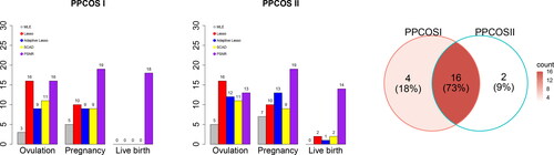
Figures 4 and 5 present the covariates associated with the three outcomes. Treatment effects are consistently identified across all stages, as we shall see later. First, the competing methods can hardly detect any signals at the stage of live birth, but benefiting from the modeling framework, the proposed method is able to uncover lasting influence at later stages. Second, influential covariates discovered by applying PSNR to the PPCOS I and PPCOS II datasets show strong consensus, but this is not the case for the other methods. The patterns are clearly illustrated in Figure 6. The number of covariates identified by the other methods remarkably drops to almost zero for live birth, whereas PSNR maintains its performance across the stages.

Fig. 4 Covariates identified by various methods. The red, green, and white blocks represent negative, positive, and no effects on the three binary outcomes, respectively.

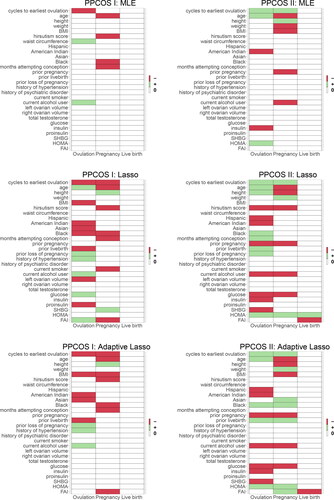
Fig. 5 Covariates identified by various methods (cont.). The red, green, and white blocks represent negative, positive, and no effects on the three binary outcomes, respectively.

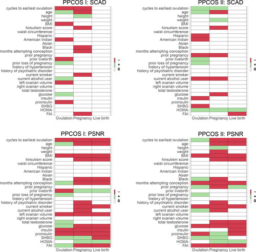
Fig. 6 The barplots show the number of covariates identified by various methods across the three stages. The Venn diagram shows the consensus between the results of the PPCOS I and PPCOS II using the proposed method.

The following patterns of the selected variables are common to the PPCOS I and PPCOS II data. From Figure 5, we see that cycle of the earliest ovulation, age, BMI, hirsutism score, and number of months of attempting conception are negatively associated with pregnancy and live birth; as compared with whites, blacks have lower rates of pregnancy; prior loss of pregnancy is only associated with lower rates of ovulation; history of psychiatric disorder and current alcohol consumption are two factors associated with lower rates of pregnancy; current smoking reduces the likelihood of pregnancy and live birth. For the laboratory obtainable biomarkers, glucose and FAI are negatively associated with pregnancy and live birth; insulin and proinsulin are negatively associated with live birth, with proinsulin further decreasing the likelihood of ovulation; SHBG is positively associated with ovulation and pregnancy; and HOMA increases the odds of pregnancy and live birth.

There are discrepancies between the patterns of the two datasets, which may be caused by differences in covariates as shown in Table 2. This difference does not necessarily suggest inconsistencies in our findings, but rather reflects the complex relationship among the covariates and outcomes. In addition to the mutual verified patterns, the PPCOS I data provide the following add-ons: prior live birth increases the likelihood of pregnancy and live birth; left ovarian volume and insulin are negatively associated with the three outcomes; SHBG is negatively associated with live birth. The PPCOS II data show that prior pregnancy increases the likelihood of ovulation and live birth, whereas total testosterone decreases the odds of pregnancy and live birth.

The observation regarding the role of the cycle of the earliest ovulation, blacks, previous pregnancy history, history of psychiatric disorder, current alcohol user/smoker, and left ovarian volume is novel from these data, but expected. Hillman et al. (2014) reported that blacks with PCOS have increased risk for metabolic syndrome and cardiovascular disease compared with whites, which may be related to the lower rates of pregnancy among black women of the PPCOS. Magnus et al. (2019) reported that the risk of miscarriage is increased after some adverse pregnancy outcomes, suggesting that previous successful pregnancy history may have positive effects on subsequent pregnancy. Psychological interventions were found to improve pregnancy rates (Hämmerli, Znoj, and Barth 2009), which appear to explain our observation regarding history of psychiatric disorder. It is well established that adverse effects of alcohol consumption on fetal health are synergistic with smoking (Wright et al. 1983), our results provide timely evidence and additional motivation to encourage smoking cessation and reducing alcohol consumption before pregnancy.

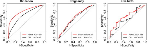
Beyond discovering associations between risk factors and the three pregnancy outcomes, it is important to develop a prognostic model to predict outcomes. This is difficult as both of the PPCOS I and PPCOS II samples have drastically decreased sample sizes and unbalanced event counts for the later outcomes. Figure 7 compares two receiver operating characteristic (ROC) curves. The red curve is derived from a prediction model built from the PPCOS I data by our proposed PSNR method and applied to the PPCOS II data for the estimation of specificity and sensitivity. See Table S2 in supplementary material for the model. The black curve is from a commonly used clinical model (denoted by CM). CM is a sequential logistic regression containing the clinically evident factors as given in Figure 2. We also evaluated a model only containing age and FAI as recommended by practitioners (Kuang et al. 2015), its performance is slightly inferior to CM and is not shown here. Figure 7 reveals that PSNR clearly outperforms CM for ovulation and live birth, and is still marginally better than CM for the outcome pregnancy.

Fig. 7 Receiver operating characteristic (ROC) curves show the predictive performance of the regression models trained on the PPCOS I dataset and applied to the PPCOS II dataset. CM: Clinical model using treatment, age, BMI, hirsutism score, and number of months of attempting conception as covariates.

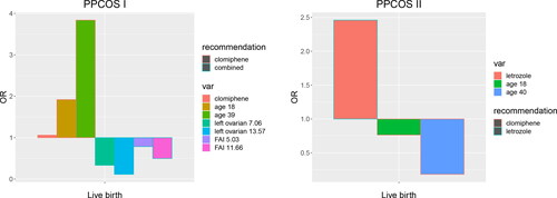
As the last step, from the perspective of precision medicine, we explore whether the treatment effect varies by potential subgroups determined by the predictors in the prognostic model as in Figure 7. To this end, we investigate interactive effects between the treatment and the predictors. We carry out a post hoc analysis by including the interaction terms and conduct variable selection through the proposed PSNR. The following interactions are identified for live birth: treatment and age, left ovarian volume, FAI, respectively, from the PPCOS I; treatment and age from the PPCOS II. Figure 8 visualizes various treatment effects on live birth as represented by odds ratio (OR). Figures S1 and S2 in supplementary material present treatment effects on ovulation and pregnancy, respectively. No interaction terms are found for metformin and it is inferior to other treatments in achieving live birth and other pregnancy outcomes.

Fig. 8 Odds ratio (OR) of treatment and subgroup effects identified by PSNR. Based on the variables that are identified to interact with the treatment, we dichotomize the patients into subgroups with low and high values of those variables. Treatment recommendations are given according to the ORs. From the PPCOS I, in terms of live birth rate, the main effects of clomiphene and combination therapy are quite close; clomiphene is more effective for older women; combination therapy is more effective for the patients with a larger left ovarian volume or FAI. From the PPCOS II, letrozole is more effective in terms of live birth rate, whereas clomiphene is more effective for older women.

We note that the treatment effects on live birth cannot be detected by any competing separate models (MLE, Lasso, adaptive Lasso, and SCAD), whereas our PSNR recognizes lasting influence on live birth despite the fact that the sample size decreased and event counts were extremely unbalanced. The detection power of the four separate models is limited as they are only able to identify the treatment effects at several early stages of pregnancy. See Figure S3 in supplementary material for details.

Second, the main effects of the treatment detected by PSNR are in agreement with the conclusions of the PPCOS trials (Legro et al. 2007, 2014).

Last but not the least, we can formulate treatment recommendations to improve live birth according to the ORs shown in Figure 8. From the PPCOS I, the main effects of clomiphene and the combination therapy are quite close; clomiphene is more effective for older women; and the combination therapy is more effective for the patients with a larger left ovarian volume or FAI. From the PPCOS II, letrozole is more effective, whereas clomiphene is more effective for older women. Interestingly, Zhang et al. (2010) suggested that left ovarian volume appears to be of great value in recommending effective treatment options. They constructed a decision tree for ovulation rate and recommended the combination therapy for those patients with larger left ovarian volumes in the PPCOS I. Our results validate their findings from a different perspective.

7 Discussion

We have developed a framework to perform joint variable selection and coefficients estimation of SNBOs. The unique structure of SNBOs leads to decreased sample sizes and possibly unbalanced event counts at later stages, which makes it difficult to detect variables that are potentially influential to later stage outcomes. Joint model that incorporates information from multiple outcomes are more powerful than modeling each outcome separately to detect associations at later stages. By borrowing the variable selection information from precedent stage outcomes, our joint estimation approach gives increased power to detect influence of covariates relative to separate models for each outcome. It is noteworthy that our method is not restricted by the ratio of sample size or the number of covariates, which allows us to consider genetic markers in future studies. One future direction is to carry the information in the early stage outcomes onto the subsequent ones in statistical inference. Another direction is variable selection taking account of SNBOs and hierarchical structures of interactions simultaneously, for example, by using decision trees seem to be natural solutions (Zhang et al. 2010). It warrants further research and development.

When applied to the PPCOS I and II data, on the one hand, our method successfully validates various important findings in the literature such as the effects of age, BMI, hirsutism score, the number of months of attempting conception, and some laboratory biomarkers. On the other hand, it discovers insightful associations and lasting influence of basic characteristics on the pregnancy outcomes which have not been revealed.

We demonstrate that the clinical covariates and laboratory biomarkers that overlap with those reported in the literature can be used to develop a prognostic model to predict a woman’s chance of having live birth. Our findings also provide evidence for patient tailored infertility treatment options.

Acknowledgments

The authors wish to thank the Reproductive Medicine Network for sharing the dataset.

Supplementary Material

Supplement: Supplement containing technical details and additional results for simulation studies and data application.

Code: Code implementing the proposed method.

Additional information

Funding

This work is supported in part by grants U10HD055925 from the National Institutes of Health.

References

- Agresti, A. (2002), Categorical Data Analysis , New York: Wiley-Interscience.
- Azziz, R. , Woods, K. S. , Reyna, R. , Key, T. J. , Knochenhauer, E. S. , and Yildiz, B. O. (2004), “The Prevalence and Features of the Polycystic Ovary Syndrome in an Unselected Population,” The Journal of Clinical Endocrinology & Metabolism , 89, 2745–2749.
- Chen, Z.-J. , Shi, Y. , Sun, Y. , Zhang, B. , Liang, X. , Cao, Y. , Yang, J. , Liu, J. , Wei, D. , Weng, N. , Tian, L. , Hao, C. , Yang, D. , Zhou, F. , Shi, J. , Xu, Y. , Li, J. , Yan, J. , Qin, Y. , Zhao, H. , Zhang, H. , and Legro, R. S. (2016), “Fresh Versus Frozen Embryos for Infertility in the Polycystic Ovary Syndrome,” New England Journal of Medicine , 375, 523–533. DOI: https://doi.org/10.1056/NEJMoa1513873.
- Dicker, L. , Huang, B. , and Lin, X. (2013), “Variable Selection and Estimation With the Seamless-l 0 Penalty,” Statistica Sinica , 23, 929–962.
- ESHRE, The Rotterdam and ASRM-Sponsored PCOS Consensus Workshop Group . (2004), “Revised 2003 Consensus on Diagnostic Criteria and Long-Term Health Risks Related to Polycystic Ovary Syndrome,” Fertility and Sterility , 81, 19–25.
- Fan, J. , and Li, R. (2001), “Variable Selection via Nonconcave Penalized Likelihood and its Oracle Properties,” Journal of the American statistical Association , 96, 1348–1360. DOI: https://doi.org/10.1198/016214501753382273.
- Fan, J. , and Lv, J. (2011), “Nonconcave Penalized Likelihood with np-Dimensionality,” IEEE Transactions on Information Theory , 57, 5467–5484. DOI: https://doi.org/10.1109/TIT.2011.2158486.
- Fox, J. (1997), Applied Regression Analysis, Linear Models, and Related Methods , Thousand Oaks, CA: Sage Publications, Inc.
- Friedman, J. , Hastie, T. , and Tibshirani, R. (2010), “Regularization Paths for Generalized Linear Models via Coordinate Descent,” Journal of Statistical Software , 33, 1–22. DOI: https://doi.org/10.18637/jss.v033.i01.
- Hämmerli, K. , Znoj, H. , and Barth, J. (2009), “The Efficacy of Psychological Interventions for Infertile Patients: A Meta-Analysis Examining Mental Health and Pregnancy Rate,” Human Reproduction Update , 15, 279–295. DOI: https://doi.org/10.1093/humupd/dmp002.
- Hansen, K. R. , He, A. L. W. , Styer, A. K. , Wild, R. A. , Butts, S. , Engmann, L. , Diamond, M. P. , Legro, R. S. , Coutifaris, C. , Alvero, R. , Robinson, R. D. , Casson, P. , Christman, G. M. , Huang, H. , Santoro, N. , Eisenberg, E. , Zhang, H. , and Eunice Kennedy Shriver National Institute of Child Health and Human Development Reproductive Medicine Network . (2016), “Predictors of Pregnancy and Live-Birth in Couples With Unexplained Infertility After Ovarian Stimulation–Intrauterine Insemination,” Fertility and Sterility , 105, 1575–1583. DOI: https://doi.org/10.1016/j.fertnstert.2016.02.020.
- Harbin Consensus Conference Workshop Group . (2014), “Improving the Reporting of Clinical Trials of Infertility Treatments (IMPRINT): Modifying the Consort Statement,” Fertility and Sterility , 102, 952–959,e15.
- Hillman, J. K. , Johnson, L. N. , Limaye, M. , Feldman, R. A. , Sammel, M. , and Dokras, A. (2014), “Black Women With Polycystic Ovary Syndrome (PCOS) have Increased Risk for Metabolic Syndrome and Cardiovascular Disease Compared With White Women With PCOS,” Fertility and Sterility , 101, 530–535. DOI: https://doi.org/10.1016/j.fertnstert.2013.10.055.
- Huang, Y. , Zhang, Q. , Zhang, S. , Huang, J. , and Ma, S. (2017), “Promoting Similarity of Sparsity Structures in Integrative Analysis With Penalization,” Journal of the American Statistical Association , 112, 342–350. DOI: https://doi.org/10.1080/01621459.2016.1139497.
- Kuang, H. , Jin, S. , Hansen, K. R. , Diamond, M. P. , Coutifaris, C. , Casson, P. , Christman, G. , Alvero, R. , Huang, H. , Bates, G. W. , Usadi, R. , Lucidi, S. , Baker, V. , Santoro, N. , Eisenberg, E. , Legro, R. S. , Zhang, H. , and Reproductive Medicine Network . (2015), “Identification and Replication of Prediction Models for Ovulation, Pregnancy and Live Birth in Infertile Women With Polycystic Ovary Syndrome,” Human Reproduction , 30, 2222–2233. DOI: https://doi.org/10.1093/humrep/dev182.
- Legro, R. S. , and Myers, E. (2004), “Surrogate End-Points or Primary Outcomes in Clinical Trials in Women With Polycystic Ovary Syndrome?” Human Reproduction , 19, 1697–1704. DOI: https://doi.org/10.1093/humrep/deh322.
- Legro, R. S. , Barnhart, H. X. , Schlaff, W. D. , Carr, B. R. , Diamond, M. P. , Carson, S. A. , Steinkampf, M. P. , Coutifaris, C. , McGovern, P. G. , Cataldo, N. A. , Gosman, G. G. , Nestler, J. E. , Giudice, L. C. , Leppert, P. C. , Myers, E. R. , and Cooperative Multicenter Reproductive Medicine Network . (2007), “Clomiphene, Metformin, or Both for Infertility in the Polycystic Ovary Syndrome,” New England Journal of Medicine , 356, 551–566. DOI: https://doi.org/10.1056/NEJMoa063971.
- Legro, R. S. , Brzyski, R. G. , Diamond, M. P. , Coutifaris, C. , Schlaff, W. D. , Casson, P. , Christman, G. M. , Huang, H. , Yan, Q. , Alvero, R. , Haisenleder, D. J. , Barnhart, K. T. , Bates, G. W. , Usadi, R. , Lucidi, S. , Baker, V. , Trussell, J. C. , Krawetz, S. A. , Snyder, P. , Ohl, D. , Santoro, N. , Eisenberg, E. , Zhang, H. , and the NICHD Reproductive Medicine. Network* (2014), “Letrozole Versus Clomiphene for Infertility in the Polycystic Ovary Syndrome, New England Journal of Medicine , 371, 119–129. DOI: https://doi.org/10.1056/NEJMoa1313517.
- Li, Z. , Wang, S. , and Lin, X. (2012), “Variable Selection and Estimation in Generalized Linear Models With the Seamless l 0 Penalty,” Canadian Journal of Statistics , 40, 745–769. DOI: https://doi.org/10.1002/cjs.11165.
- Maddala, G. S. (1986), Limited-dependent and Qualitative Variables in Econometrics , (Vol. 3), Cambridge, UK: Cambridge University Press.
- Magnus, M. C. , Wilcox, A. J. , Morken, N.-H. , Weinberg, C. R. , and Håberg, S. E. (2019), “Role of Maternal Age and Pregnancy History in Risk of Miscarriage: Prospective Register Based Study,” British Medical Journal , 364, l869. DOI: https://doi.org/10.1136/bmj.l869.
- Rausch, M. E. , Legro, R. S. , Barnhart, H. X. , Schlaff, W. D. , Carr, B. R. , Diamond, M. P. , Carson, S. A. , Steinkampf, M. P. , McGovern, P. G. , Cataldo, N. A. , Gosman, G. G. , Nestler, J. E. , Giudice, L. C. , Leppert, P. C. , Myers, E. R. , Coutifaris, C. , and for the Reproductive Medicine Network . (2009), “Predictors of Pregnancy in Women with Polycystic Ovary Syndrome,” The Journal of Clinical Endocrinology & Metabolism , 94, 3458–3466.
- Schwarz, G. (1978), “Estimating the Dimension of a Model,” The Annals of Statistics , 6, 461–464. DOI: https://doi.org/10.1214/aos/1176344136.
- Shi, X. , Liu, J. , Huang, J. , Zhou, Y. , Shia, B. , and Ma, S. (2014), “Integrative Analysis of High-Throughput Cancer Studies With Contrasted Penalization,” Genetic Epidemiology , 38, 144–151. DOI: https://doi.org/10.1002/gepi.21781.
- Tibshirani, R. (1996), “Regression Shrinkage and Selection via the Lasso,” Journal of the Royal Statistical Society, Series B, 58, 267–288. DOI: https://doi.org/10.1111/j.2517-6161.1996.tb02080.x.
- Tutz, G. (1991), “Sequential Models in Categorical Regression,” Computational Statistics & Data Analysis , 11, 275–295.
- Wright, J. , Barrison, I. , Lewis, I. , MacRae, K. , Waterson, E. , Toplis, P. , Gordon, M. , Morris, N. , and Murray-Lyon, I. (1983), “Alcohol Consumption, Pregnancy, and Low Birthweight,” The Lancet , 321, 663–665. DOI: https://doi.org/10.1016/S0140-6736(83)91964-5.
- Wu, X.-K. , Stener-Victorin, E. , Kuang, H.-Y. , Ma, H.-L. , Gao, J.-S. , Xie, L.-Z. , Hou, L.-H. , Hu, Z.-X. , Shao, X.-G. , Ge, J. , Zhang, J. F. , Xue, H. Y. , Xu, X. F. , Liang, R. N. , Ma, H. X. , Yang, H. W. , Li, W. L. , Huang, D. M. , Sun, Y. , Hao, C. F. , Du, S. M. , Yang, Z. W. , Wang, X. , Yan, Y. , Chen, X. H. , Fu, P. , Ding, C. F. , Gao, Y. Q. , Zhou, Z. M. , Wang, C. C. , Wu, T. X. , Liu, J. P. , Ng, E. H. Y. , Legro, R. S. , Zhang, H. , and PCOSAct Study Group . (2017), “Effect of Acupuncture and Clomiphene in Chinese Women With Polycystic Ovary Syndrome: A Randomized Clinical Trial,” Journal of American Medical Association , 317, 2502–2514. DOI: https://doi.org/10.1001/jama.2017.7217.
- Yuan, M. , and Lin, Y. (2006), “Model Selection and Estimation in Regression With Grouped Variables,” Journal of the Royal Statistical Society, Series B, 68, 49–67. DOI: https://doi.org/10.1111/j.1467-9868.2005.00532.x.
- Zhang, C.-H. (2010), “Nearly Unbiased Variable Selection Under Minimax Concave Penalty,” The Annals of Statistics , 38, 894–942. DOI: https://doi.org/10.1214/09-AOS729.
- Zhang, H. , Legro, R. S. , Zhang, J. , Zhang, L. , Chen, X. , Huang, H. , Casson, P. R. , Schlaff, W. D. , Diamond, M. P. , Krawetz, S. A. , Coutifaris, C. , Brzyski, R. G. , Christman, G. M. , Santoro, N. F. , and Eisenberg, E. (2010), “Decision Trees for Identifying Predictors of Treatment Effectiveness in Clinical Trials and its Application to Ovulation in a Study of Women With Polycystic Ovary Syndrome,” Human Reproduction , 25, 2612–2621. DOI: https://doi.org/10.1093/humrep/deq210.
- Zhao, P. , and Yu, B. (2006), “On Model Selection Consistency of Lasso,” The Journal of Machine Learning Research , 7, 2541–2563.
- Zhao, P. , Rocha, G. , and Yu, B. (2009), “The Composite Absolute Penalties Family for Grouped and Hierarchical Variable Selection,” The Annals of Statistics , 37, 3468–3497. DOI: https://doi.org/10.1214/07-AOS584.
- Zou, H. (2006), “The Adaptive Lasso and its Oracle Properties,” Journal of the American Statistical Association , 101, 1418–1429. DOI: https://doi.org/10.1198/016214506000000735.