A Multimodal Multilevel Neuroimaging Model for Investigating Brain Connectome Development

Abstract

Recent advancements of multimodal neuroimaging such as functional MRI (fMRI) and diffusion MRI (dMRI) offers unprecedented opportunities to understand brain development. Most existing neurodevelopmental studies focus on using a single imaging modality to study microstructure or neural activations in localized brain regions. The developmental changes of brain network architecture in childhood and adolescence are not well understood. Our study made use of dMRI and resting-state fMRI imaging data sets from Philadelphia Neurodevelopmental Cohort (PNC) study to characterize developmental changes in both structural as well as functional brain connectomes. A multimodal multilevel model (MMM) is developed and implemented in PNC study to investigate brain maturation in both white matter structural connection and intrinsic functional connection. MMM addresses several major challenges in multimodal connectivity analysis. First, by using a first-level data generative model for observed measures and a second-level latent network modeling, MMM effectively infers underlying connection states from noisy imaging-based connectivity measurements. Second, MMM models the interplay between the structural and functional connections to capture the relationship between different brain connectomes. Third, MMM incorporates covariate effects in the network modeling to investigate network heterogeneity across subpopoulations. Finally, by using a module-wise parameterization based on brain network topology, MMM is scalable to whole-brain connectomics. MMM analysis of the PNC study generates new insights in neurodevelopment during adolescence including revealing the majority of the white fiber connectivity growth are related to the cognitive networks where the most significant increase is found between the default mode and the executive control network with a 15% increase in the probability of structural connections. We also uncover functional connectome development mainly derived from global functional integration rather than direct anatomical connections. To the best of our knowledge, these findings have not been reported in the literature using multimodal connectomics. Supplementary materials for this article, including a standardized description of the materials available for reproducing the work, are available as an online supplement.

KEYWORDS:

• Brain connectome
• dMRI
• fMRI
• Multilevel model
• Multimodal neuroimaging
• Network modeling

1 Introduction

In recent neuroscience research, there has been significant increase of interest on brain connectome analysis for understanding brain organizations and their alterations due to neurodevelopment or brain-related diseases. In particular, with the advances of imaging technologies, different imaging modalities including the anatomical and the functional imaging offer unprecedented opportunities for investigating the development of brain structural and functional connections during brain maturation. Neuroimaging studies have investigated brain white matter structural changes during neurodevelopment using diffusion magnetic resonance imaging (dMRI) (Krogsrud et al. 2016). Investigators mainly focused on studying changes in white matter microstructure captured by diffusion tensor imaging (DTI) summary measures including fractional anisotropy (FA), mean diffusivity (MD), and radial diffusivity (RD) whichreflect water diffusion patterns in localized white matter regions. Other studies investigated brain functional changes using functional MRI (fMRI) (Rubia et al. 2000). Investigators mainly focused on studying the effects of age on task-related brain activations related to cognitive processes such as language development, inhibitory control and executive functioning. Though recent neuroimaging studies have generated important findings in brain development, there are two major limitations in current neurodevelopmental research. First, existing studies largely focus on studying developmental changes in white matter structure or brain activations in localized brain regions. More studies are needed to investigate neurodevelopment in network connections between regions across the brain. Second, existing studies mostly focus on single imaging modality investigation on either structural or functional development. Very limited work has been done to jointly consider the development of structural and functional connections among children and adolescents. Multimodal connectivity analysis has great potentials in filling the gap in current neurodevelopmental studies. Specifically, temporal coherence present in resting-state fMRI are believed to reflect the intrinsic functional connectivity (FC) of the brain. dMRI tractography is widely used now to infer underlying white matter fiber tracts for structural connectivity (SC) across the brain. By combining SC and FC information derived from dMRI and fMRI on the same individuals, multimodal connectivity analysis helps reveal the interplay between the brain structural connection maturation and function integration during the neurodevelopment, which is of paramount importance in more comprehensive understanding of brain maturation.

In the neuroscience literature, methods have been proposed to analyze dMRI and fMRI data together in order to exploit complementary information from different modalities. There has been work in using fMRI data to help fiber tracking and fiber filtering in dMRI data analysis and work in using dMRI data to better characterize functional connectivity (Zhu et al. 2014) or help understand the reproducibility of functional networks (Kemmer et al. 2018). There are also abundance of methods for incorporating SC metrics derived from dMRI data in FC analysis to improve the accuracy for estimating functional networks (Hinne et al. 2014; Higgins, Kundu, and Guo 2018).

Despite the existing multimodal methods, inferring the relationship between brain structural and functional connections based on observed multimodal images in neurodevelopment studies still remains a challenging task. Although existing evidence shows the role of white matter fiber tracts in regulating FC (Sporns 2013), the structure-function relationship is not deterministic but rather quite complex. For example, strong SC can predict higher functional correlations while the converse does not hold (Honey et al. 2009). It was found that structural connectivity alone only accounts for a small proportion of FC variance. Current understanding is that FC not only derives from structural connections but may also generate from unobservable dynamics in neuronal activity (Bressler and Tognoli 2006) and or result from hierarchical integration of brain functional networks (Mastrandrea et al. 2017). Additionally, given the well-known low signal-to-noise ratio of MRI and the limitations of imaging processing procedures, the FC and SC estimated from the observed fMRI and dMRI data usually contains considerable random variations in reflecting underlying functional and structural connections. Furthermore, the brain connections are altered by neurodevelopment. These challenges call for statistical methods that can effectively and reliably characterize brain functional and structure connections and their relationship, with the ability to accommodate and assess the heterogeneity across subpopulations.

The needs to develop such statistical methods for multimodal connectivity analysis are demonstrated by the Philadelphia Neurodevelopmental Cohort (PNC) study. The PNC study is a large-scale research initiative funded by National Institute of Mental Health, aiming to understand how brain maturation and how various factors affect the neurodevelopment and development of cognition (Satterthwaite et al. 2014). The cohort consists of youths aged 8–21 years who went to the Children’s Hospital of Philadelphia for a pediatric visit and volunteered to participate in genomic studies of complex pediatric disorders. Brain images were acquired for a subset of the participants in the PNC study and included multiple modalities such as T1 weighted MRI, resting-state fMRI (rs-fMRI) and dMRI. A research goal in assessing the neurodevelopment is to investigate how structural and functional connections are altered during neurodevelopment and whether there is dependence between their changes when kids grow up. Given the wide spectrum of functions that the brain controls, it is also of great interest to understand whether and how the neurodevelopment occurs in different manners for various types of brain networks. For example, it is interesting to compare the neurodevelopment of the lower-level networks involved in sensory and motor functions versus the higher-order cognitive networks involved in sophisticated cognitive functioning such as decision making and emotion regulation. Furthermore, it is important to control for potential confounding factors such as gender in the multimodal connectivity analysis of neurodevelopment.

In this article, we develop a multimodal multilevel model (MMM) to conduct multimodal connectomics using dMRI and rs-fMRI in the PNC study to investigate neurodevelopment in structural and functional network architecture. MMM uses a population-level latent network modeling to model latent functional and structural connectivity states representing the underlying brain connectomes. MMM then includes data generative models to model the observed FC and SC data across subjects based on the population-level latent connection states. The data generative models help account for the measurement variations and between-subject variability in the observed FC and SC metrics. MMM models the relationship between structural and functional connectivity in both the latent network modeling as well as the data generative models to capture the complex relationship between FC and SC. Furthermore, MMM allows assessing covariate effects on brain connections, which captures brain network differences between age and gender groups in the PNC study.

One common challenge in brain network modeling is the large number of edges in the network. Edge-specific parameterization in network modeling results in enormous numbers of parameters to be estimated from the data, which is computationally expensive or even infeasible in some cases. To address this issue, some existing multimodal network models (Venkataraman et al. 2012) assume common parameters to characterize the strength of connections across all edges in the whole brain network. This whole-network parameterization scheme doesn’t take into account the modular structure in brain network topology where within-modules nodes are highly inter-connected and between-module connections are relatively sparse (Meunier, Lambiotte, and Bullmore 2010). Furthermore, the whole-network parameterization is too simple to capture the differences across various subnetworks in the brain and has limited capacity to provide a good fit to the observed connections. In this article, we propose a module-wise parameterization for the latent network modeling of MMM. The module-wise parameterization takes into account the well-established intrinsic subnetwork structure in brain network topology (Smith et al. 2009) and specifies module-specific parameters for the edges based on the module memberships of the nodes. Compared with the edge-specific and whole-network parameterization, the proposed module-wise parameterization has the advantage of providing a great balance between computational efficiency and precision by exploiting the modularity of the brain network. This makes MMM scalable to whole brain connectomic analysis for a comprehensive view of neurodevelopment in the brain while at the same time provides MMM the precision to detect how neurodevelopment varies across different brain modules, for example, cognitive versus sensory networks. We develop an EM algorithm for estimating the parameters in the MMM and develop a statistical inference procedure based on parameteric bootstrap to test covariates effects on brain connections.

Application of the MMM to the FC and SC measures from rs-fMRI and dMRI data in the PNC study leads to new insightful findings about age-related differences in brain functional and structure connections. Specifically, we find a general increase in white fiber structural connections across the brain with the increase in age. In particular, MMM results reveal that the increase in white matter fiber connection is more significant for higher-order cognitive networks such as the default mode network, executive control network and frontal parietal networks as compared to lower-order sensory and motor networks. In particular, we find the most significant white matter connection increase occurs between the default mode and the executive control network where there is a 15% increase in the probability of structural connections from the age group of 8–15 to the age group of 16–21. MMM also reveals that the brain becomes more functionally ordered or connected during adolescence. In particular, with the increase of age, we find a significant increase in the positive FC between the sensorimotor network and lateral visual and auditory network. Furthermore, through MMMs joint modeling of FC and SC, we obtain new insights that functional connection development during adolescence mainly happens at long-range edges and edges that are functionally integrated not by direct anatomical connections but rather via the global brain hierarchical organization. In addition to neurodevelopment, neural connectivity also plays an important role in brain diseases. Recent findings have shown that many mental disorders and neurodevelopmental disorders are caused by disrupted neural connections among certain brain circuits (Williams 2016; Henry and Cohen 2019). The proposed MMM method provides an advanced analytical tool for investigating the associations between disruptions in brain networks and brain diseases.

The remainder of the article is organized as follows. The framework of MMM is presented in Methods section, which includes the model specification, estimation by EM algorithm, and inference procedure. We then perform a multimodal connectivity analysis of the PNC study with MMM and report detailed findings. Additionally, we conduct simulation studies to evaluate the proposed method in terms of the accuracy of the estimation and validity of the inference procedure. Conclusion and discussions are presented in the last section.

2 Methods

2.1 A Multimodal Multilevel Model (MMM)

The MMM aims to jointly model the functional and structural connections estimated from multimodal imaging including fMRI and dMRI. Specifically, functional connections are defined as the temporal coherence between the fMRI blood-oxygen-level-dependent (BOLD) series of spatially disjoint brain regions, which is often quantified using functional connectivity (FC) correlations. Structural connections represent anatomical connections via white matter fiber bundles and are commonly measured by the probability of structural connectivity (SC) obtained from diffusion tractography on dMRI data. Prior to the modeling, some proper transformations are typically performed on the FC and SC measures, for example, to change the range into the entire real line. Suppose we have I subjects in total from G subgroups with I_g subjects in gth group and we are considering connections between Q regions or nodes in the brain. Let $R_{jk,g,i_g}$ and $D_{jk,g,i_g}$ denote the transformed FC and SC measure capturing the functional and structural connectivity, respectively, between the jth and kth node for subject i in the gth group, with $j\ne k,j,k=1,\dots ,Q$ and $i_g=1,\dots ,I_g$. These FC and SC metrics are based on observed fMRI and dMRI imaging data and often measured with errors (Côté et al. 2013; Liu 2016; Zalesky et al. 2016). To infer the underlying brain connections from the observed data, we introduce latent structural and functional connectivity indicators for a given population. Specifically, $A_{jk,g}$ is a binary latent indicator representing the latent structural or anatomical connectivity between the jth and kth node for the gth group. $A_{jk,g}$ indicates whether or not there are white matter fiber bundles connecting the two regions. $F_{jk,g}$ is a tri-state latent variables taking values of $1,0,-1$ indicating two regions have positive functional connection, no functional connections or negative functional connections, respectively.

In MMM, we propose a multi-level modeling scheme where the first level of MMM models the observed FC and SC data across subjects in terms of the population-level latent connectivity states and the second level of MMM models the latent functional and structural connectivity states for various subpopulations. In the first level of MMM, we model the observed FC and SC metrics, that is, $R_{jk,g,i_g}$ and $D_{jk,g,i_g}$, in terms of the latent connectivity states, that is, $A_{jk,g}$ and $F_{jk,g}$. The data generative models are specified based on the characteristics of empirical distributions of the observed FC and SC. Specifically, for the SC metric based on the diffusion tractography, there are usually a considerable number of node pairs for which zero connecting tracts are found from the probabilistic tractography, that is, $D_{jk,g,i_g}$ is set to 0, and the rest of the node pairs have a varying number of connecting tracts. Given the latent structural connectivity state $A_{jk,g}=u$ with $u\in \{0,1\}$, we propose the following model for the observed SC measure,(1) $$D_{jk,g,i_g}|A_{jk,g}=u\sim {\rho }^u\delta (D_{jk,g,i_g})+(1-{\rho }^u)Mo{G}^u,$$(1) where $\delta (·)$ is the Dirac delta function and $Mo{G}^u={\sum }_{l=1}^L{\gamma }_l^{u}f(D_{jk,g,i_g};{\chi }_l^u,{({\xi }_l^u)}^2)$ represents a Mixture of Gaussian (MoG) distribution with L Gaussian components where $0<{\gamma }_l^u<1$ and ${\sum }_l^L{\gamma }_l^u=1,f(·)$ is the pdf of Gaussian distribution, and ${\chi }_l^u$ and ${({\xi }_l^u)}^2$ are the mean and variance parameters. L = 3 is usually sufficient based on the empirical distribution of the SC measures. Latent labels are often introduced to facilitate derivations in models involving MoG. We define MoG latent labels ${\left\{{\tau }_{jk,g,i_g,l}\right\}}_{l=1}^L$ that take value in {0, 1} with ${\sum }_{l=1}^L{\tau }_{jk,g,i_g,l}=1$ and $p({\tau }_{jk,g,i_g,l}=1)={\gamma }_l^u$. In (1), the Dirac delta captures the scenario that a node pair ends up with zero connecting tracts in tractography and the MoG describes the distribution of the probability of SC when the tractography generates connecting tracts for a node pair. The parameter ρ^u($u\in \{0,1\}$), controls the relative weight of the Dirac delta and the MoG in the overall distribution. Given that dMRI imaging and tractography uses imaging and computational algorithm to indirectly measure underlying water diffusion patterns and reconstruct fiber tracts, the observed SC measure is a noisy measurement of the underlying structural connection. Therefore, it is likely that the tractography doesn’t generate connecting tracts for node pairs with underlying structural connections, and generate tracts for node pairs without underlying structural connection (Côté et al. 2013; Zalesky et al. 2016). The parameter ρ^u ($u\in \{0,1\}$), which is between 0 and 1, helps account for the variation of the observed data due to the noise in imaging measurements and the uncertainty from the tractography algorithm. It is worth noting that ρ^u depends on $A_{jk,g}$ because the relative weight is expected to vary depending on the underlying connection status where lower weight of the Dirac delta is generally expected for node pairs with white matter fiber bundles connections.

We propose the following Gaussian model for the observed FC measure given latent structural connectivity state $A_{jk,g}=u$ ($u\in \{0,1\}$) and the latent functional connectivity state $F_{jk,g}=v$ ($v\in \{1,0,-1\}$),(2) $$R_{jk,g,i_g}|A_{jk,g}=u,F_{jk,g}=v\sim N({\mu }^{u,v},{({\sigma }^{u,v})}^2),$$(2)

The choice of Gaussian distribution model for FC measures is motivated by the empirical distribution of the observed FC metrics. The parameters of the Gaussian distribution in (2) depends on both the latent structural connectivity state $A_{jk,g}$ and the latent functional connectivity state $F_{jk,g}$. This is to help better capture the complex relationship between the functional and structural connections. That is, FC is only partially dependent on direct fiber bundle connections and is also affected by other factors such as unobservable dynamics in the underlying neuronal activity or hierarchical integration of brain functional networks (Mastrandrea et al. 2017).

The second-level of MMM is latent network modeling of the underlying structural and functional connectivity states for the edges. To achieve a good balance between computational efficiency and precision for modeling the large number of edges in the brain, we exploit the well-established intrinsic module system in the brain (Smith et al. 2009) and propose a module-wise parameterization for the latent network modeling. Specifically, we specify module-specific parameters for the edges based on the module memberships of the node pairs. Furthermore, we specify group-specific parameters to capture and examine the network differences between subpopulations with varying clinical and demographic characteristics. We model the binary latent structural connectivity state variable between jth and kth node ($j<k,j,k=1,\dots ,Q$) for the gth ($g=1,\dots ,G$) subject group as follows,(3) $$\begin{array}{c}{A}_{jk,g}\sim \text{Bernoulli}({\pi }_{m(j)m(k),g}),\\ \text{with}\hspace{1em}\text{logit}({\pi }_{m(j)m(k),g})={\mathit{x}}_g^T{\mathit{\beta }}_{m(j)m(k)},\end{array}$$(3) where m(j) and m(k) is the module membership of jth and kth node with $m(j),m(k)\in \{1,\dots ,M\}$ and M is the total number of modules in the brain network, ${\mathit{x}}_g$ represents the covariates patterns characterizing the gth subject group, ${\mathit{\beta }}_{m(j)m(k)}$ captures the covariate effects on the latent structural connectivity states.

We model the tri-state latent functional connectivity between jth and kth node for gth subject group using a multinomial logit model where the parameters depend on the latent structural connectivity state. As in the latent structural connectivity model, the parameters in the functional model are also module-specific and group-specific. Given $A_{jk,g}=u(u=0,1)$, we have(4) $$F_{jk,g}|A_{jk,g}=u\sim \text{Multinomial}({\mathit{p}}_{m(j)m(k),g}^u),$$(4) where ${\mathit{p}}_{m(j)m(k),g}^u=(p_{m(j)m(k),g}^{u,1},p_{m(j)m(k),g}^{u,0},p_{m(j)m(k),g}^{u,-1})$ are the multinomial parameters with $p_{m(j)m(k),g}^{u,v}$ $(v=1$, 0, $-1)$ corresponding to the probability for positive connection, no connection and negative connection, respectively, and that $\sum _v{p}_{m(j)m(k),g}^{u,v}=1$. We specify the no connection state, that is, j = 0, as the reference level and model the log-odds in terms of covariates,(5) $$\begin{array}{c}\hspace{0.17em}\text{log}\hspace{0.17em}(\frac{p_{m(j)m(k),g}^{u,1}}{p_{m(j)m(k),g}^{u,0}})={\mathit{x}}_g^T{\mathit{\alpha }}_{m(j)m(k)}^{u,1},\\ \hspace{0.17em}\text{log}\hspace{0.17em}(\frac{p_{m(j)m(k),g}^{u,-1}}{p_{m(j)m(k),g}^{u,0}})={\mathit{x}}_g^T{\mathit{\alpha }}_{m(j)m(k)}^{u,-1}\end{array}$$(5) where ${\mathit{\alpha }}_{m(j)m(k)}^{u,1}$ and ${\mathit{\alpha }}_{m(j)m(k)}^{u,-1}$ captures the covariate effects on the latent functional connectivity states.

To provide an overview of the MMM modeling framework, we present a schematic diagram in Figure 1 and summarize the parameters in MMM in Table 1.

Fig. 1 A schematic representation of the MMM modeling framework.

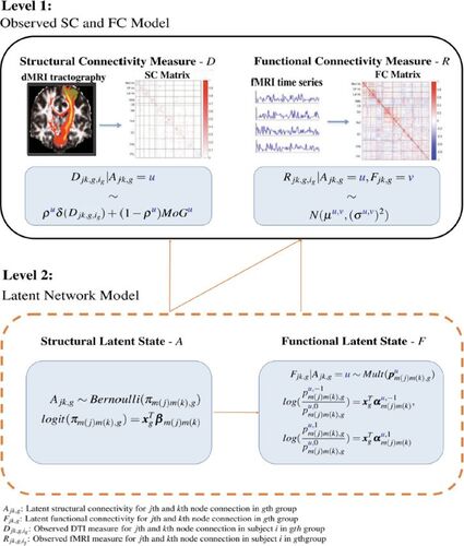
Table 1 Important symbols and parameters in the model.

$A_{jk,g}$	Latent structural connectivity for jth and kth node connection in gth group
$F_{jk,g}$	Latent functional connectivity for jth and kth node connection in gth group
$D_{jk,g,i_g}$	Observed dMRI measure for jth and kth node connection in subject i in gth group
$R_{jk,g,i_g}$	Observed fMRI measure for jth and kth node connection in subject i in gth group
${\mathbf{\Theta }}_1$	$\mathit{\beta },{\mathit{\alpha }}^{u,-1},{\mathit{\alpha }}^{u,1}$: Covariate effects parameters in latent network modeling (level 2)
${\mathbf{\Theta }}_2$	ρ^u, ${\gamma }_l^u,{\chi }_l^u,{({\xi }_l^u)}^2$: SC related parameters (level 1)
${\mathbf{\Theta }}_3$	${\mu }^{u,v},{({\sigma }^{u,v})}^2$: FC related parameters (level 1)

2.2 Maximum Likelihood Estimation and the EM Algorithm

We develop a maximum likelihood (ML) estimation method via EM algorithm for estimating the parameters and inferring the latent variables in the proposed MMM. Based on (1)–(4) and assuming the independence of the latent and observed variables, the complete data log-likelihood for MMM can be represented as(6) $$l_C(\mathbf{\Theta };\mathcal{D},\mathcal{R},\mathcal{A},\mathcal{F},\mathcal{T})=\sum _{g=1}^G\sum _{j=1}^{Q-1}\sum _{k:j<k}{l}_{jk,g}(\mathbf{\Theta };\mathcal{D},\mathcal{R},\mathcal{A},\mathcal{F},\mathcal{T}),$$(6) where $\mathbf{\Theta }=\{{\mathbf{\Theta }}_1,{\mathbf{\Theta }}_2,{\mathbf{\Theta }}_3\}$ includes the parameters, $\mathcal{D}=\left\{D_{jk,g,i_g}\right\}$, $\mathcal{R}=\left\{R_{jk,g,i_g}\right\}$ are observed SC and FC measures derived from dMRI and fMRI data across subjects, $\mathcal{A}=\left\{A_{jk,g}\right\}$ and $\mathcal{F}=\left\{F_{jk,g}\right\}$ represents latent structural and functional connectivity states, respectively, and $\mathcal{T}=\left\{{\tau }_{jk,g,i_g,l}\right\}$ represents latent labels for the mixture of Gaussian distribution for modeling the observed SC measures.

The detailed expression of $l_{jk,g}$ in the complete data log-likelihood is as follows:(7) $$\begin{array}{c}{l}_{jk,g}(\mathbf{\Theta };\mathcal{D},\mathcal{R},\mathcal{A},\mathcal{F},\mathcal{T})=\sum _{u=0}^1\sum _{v=-1}^1\mathbb{I}(A_{jk,g}=u,F_{jk,g}=v)\\ \times \hspace{0.17em}\text{log}\hspace{0.17em}\{{\Psi }_{jk,g}^{u,v}({\mathbf{\Theta }}_1)\prod _{i_g=1}^{I_g}{\varphi }^{u,v}\\ (D_{jk,g,i_g},R_{jk,g,i_g}{\tau }_{jk,g,i_g,l}|{\mathbf{\Theta }}_2,{\mathbf{\Theta }}_3)\},\end{array}$$(7) where$$\begin{array}{cc}\hfill & {\Psi }_{jk,g}^{u,v}({\mathbf{\Theta }}_1)={({\pi }_{m(j)m(k),g}^{\alpha })}^u{(1-{\pi }_{m(j)m(k),g}^{\alpha })}^{1-u}{p}_{m(j)m(k),g}^{u,v},\hfill \\ \hfill & {\varphi }^{u,v}(D_{jk,g,i_g},R_{jk,g,i_g},{\tau }_{jk,g,i_g,l}|{\mathbf{\Theta }}_2,{\mathbf{\Theta }}_3)\hfill \\ \hfill & =[{\rho }^u\delta (D_{jk,g,i_g})+(1-{\rho }^u)\hfill \\ \hfill & \hspace{1em}\times (\sum _{l=1}^L{\gamma }_l^u{\tau }_{jk,g,i_g,l}f(D_{jk,g,i_g};{\chi }_l^u,{({\xi }_l^u)}^2)]\hfill \\ \hfill & \hspace{1em}\times f(R_{jk,g,i_g};{\mu }^{u,v},{({\sigma }^{u,v})}^2).\hfill \end{array}$$

In (7), $\mathbb{I}$ is an indicator function, ${\mathbf{\Theta }}_1=\{\mathit{\alpha },\mathit{\beta }\}$ represents the subset of parameters related to covariate effects in the second-level latent network modeling of MMM, ${\mathbf{\Theta }}_2$ and ${\mathbf{\Theta }}_3$ represents the parameters in the SC and FC data generative model in (1) and (2), respectively (Table 1).

Since our likelihood function involves unobserved latent variables, we develop an expectation-maximization (EM) algorithm for finding the maximum likelihood estimates of parameters.

E-step: In the E-step, given the parameter estimates ${\widehat{\mathbf{\Theta }}}^{(t)}$ from the last step, we derive the conditional expectation of the complete data log-likelihood given the observed data as follows:(8) $$\begin{array}{c}Q(\mathbf{\Theta }|{\widehat{\mathbf{\Theta }}}^{(t)})=\sum _{g=1}^G\sum _{j=1}^{Q-1}\sum _{k:j<k}{E}_{\mathcal{A},\mathcal{F},\mathcal{T}|\mathcal{D},\mathcal{R},{\widehat{\mathbf{\Theta }}}^{(t)}}\\ \hspace{1em}\left[l_{jk,g}(\mathbf{\Theta };\mathcal{D},\mathcal{R},\mathcal{A},\mathcal{F},\mathcal{T})\right],\end{array}$$(8)

The detailed definition of $Q(\mathbf{\Theta }|{\widehat{\mathbf{\Theta }}}^{(t)})$ is presented in Section 1 of the supplementary materials. We derive an explicit analytic form for the conditional expectation in (8). The E-step is fully tractable without the need for iterative numerical integration. The derivations can be found in Section 1.1 of the supplementary materials.

M-step: In the M-step, we update the parameters estimates as,(9) $${\widehat{\mathbf{\Theta }}}^{(t+1)}={\text{argmax}}_{\mathbf{\Theta }}Q(\mathbf{\Theta }|{\widehat{\mathbf{\Theta }}}^{(t)}).$$(9)

We also derive explicit formulas for all parameter updates except for ${\mathbf{\Theta }}_1$ which can be updated by an iterative algorithm such as the Newton–Raphson method or iteratively reweighted least squares. The details are provided in Section 1.2 of the supplementary materials.

In practice, one may potentially encounter challenges in obtaining finite solutions for ${\mathbf{\Theta }}_1$ during the ML estimation due to the complete separation or quasi-complete separation issue (Albert and Anderson 1984), especially in small sample case. This is a well-known problem for the logistic or multinomial logit model. It happens when one or more covariates can perfectly (or nearly perfect) predict the outcome variable. Some techniques have been presented to deal with the separation issue. One of the most popular techniques for solving this issue is Firth’s method, which introduces a modified score function. If we denote log-likelihood function as l, likelihood function as L, the Fisher Information for the parameters in logistic regression model as H and the determinant of H as $\left|H\right|$, the solution of the modified score function is a stationary point of a modified log-likelihood function $l^{*}=l+\frac{1}{2}\text{log}\hspace{0.17em}(|H|)$, which is equivalent to the penalized likelihood with the Jeffreys’ invariant prior as penalty $L^{*}=L*|H{|}^{\frac{1}{2}}$ (Firth 1993). Bull, Mak, and Greenwood (2002) extended this method to deal with the separation issue in multinomial logit modeling. Motivated by previous work, we propose to modify our complete log-likelihood function in (6) by adding a similar penalty term. Specifically, we propose the following penalized log-likelihood function,(10) $$\begin{array}{c}{l}_C^{*}(\mathbf{\Theta };\mathcal{D},\mathcal{R},\mathcal{A},\mathcal{F},\mathcal{T})=\sum _{g=1}^G\sum _{j=1}^{Q-1}\sum _{k:j<k}{l}_{jk,g}(\mathbf{\Theta };\mathcal{D},\mathcal{R},\mathcal{A},\mathcal{F},\mathcal{T})\\ \hspace{1em}+l_P(\mathbf{\Theta };\mathcal{D},\mathcal{R}),\end{array}$$(10) where $l_P(\mathbf{\Theta },\mathcal{D},\mathcal{R})$ is the penalty term defined as,(11) $$\begin{array}{c}{l}_P(\mathbf{\Theta },\mathcal{D},\mathcal{R})=\sum _{m_1=1}^M\sum _{m_2=1}^M\frac{1}{2}\hspace{0.17em}\text{log}\hspace{0.17em}(|{\mathbf{S}}_{m_1{m}_2}|)\\ \hspace{1em}+\sum _{m_1=1}^M\sum _{m_2=1}^M\sum _{u=0}^1\frac{1}{2}\hspace{0.17em}\text{log}\hspace{0.17em}(|{\mathbf{T}}_{m_1{m}_2}^u|).\end{array}$$(11)

Here, m₁, m₂ represent the module memberships and u represents the latent structural state. ${\mathbf{S}}_{m_1{m}_2}$ and ${\mathbf{T}}_{m_1{m}_2}^u$ play the same role as the Fisher Information matrix does in Firth’s method. ${\mathbf{S}}_{m_1{m}_2}$ serves as the correction term for latent structural states estimation and ${\mathbf{T}}_{m_1{m}_2}^u$ serves as the correction term for latent functional states estimation. Their expressions are also very close to the Fisher Information matrix in logistic regression and multinomial regression, respectively. Detailed expressions can be found in Section 2 of the supplementary materials.

With this modification, we are able to obtain finite maximum likelihood estimator and reliable estimator in the case of complete separation and quasi-complete-separation. In addition, we would still be able to perform the EM algorithm to solve for the maximum likelihood estimation by modifying the Q function in the E-step based on the penalized log-likelihood function in (10). The modified $Q^{*}$ is derived as follows,(12) $$Q^{*}(\mathbf{\Theta }|{\widehat{\mathbf{\Theta }}}^{(t)})=Q(\mathbf{\Theta }|{\widehat{\mathbf{\Theta }}}^{(t)})+l_P(\mathbf{\Theta },\mathcal{D},\mathcal{R}).$$(12)

In M-step, we adopt following procedures to update parameters. We can update ${\mathbf{\Theta }}_2$ and ${\mathbf{\Theta }}_3$ using the same updating formulas in Section 1.2 of the supplementary materials. Then, we adopt the iterative algorithm in Bull, Mak, and Greenwood (2002) to update ${\mathbf{\Theta }}_1$.

Typically, statistical inference after EM algorithm is conducted by inverting the information matrix to estimate the variance-covariance matrix of ML estimates of the parameters (Louis 1982). However, this approach is computationally challenging for MMM given the large number of parameters in the brain network modeling. Therefore, we propose to use a parameteric bootstrap method to investigate the significance of covariates effects on brain connectivity. Specifically, we first use the EM algorithm to obtain parameter estimates for the MMM and then generate bootstrap samples based on estimated MMM. We then conduct statistical inference on model parameters based on bootstrap variance estimates and apply the bootstrap functional delta method (Van Der Vaart and Wellner 1996) for hypothesis testing of functions of model parameters.

3 MMM Analysis of the PNC Study

We analyzed the multimodal imaging data from the PNC study using the proposed MMM method to investigate changes in brain functional and structural networks during neurodevelopment. The PNC study was a collaborative project between the University of Pennsylvania and the Children’s Hospital of Philadelphia (CHOP). The study included a population-based sample of over 9500 individuals aged 8–21 years selected among those who received medical care at the Children’s Hospital of Philadelphia network in the greater Philadelphia area. The sample was stratified by sex, age, and ethnicity. A subset of participants from the PNC were recruited for a multimodal neuroimaging study which included resting-state fMRI (rs-fMRI) and diffusion magnetic resonance imaging (dMRI). In this article, 881 participants’ brain images from PNC study that were downloaded from the dbGaP database. Compared with other large-scale publicly available imaging datasets, the PNC data has a major advantage that all the images were acquired on a single MRI scanner using the same scanning protocol, without variations from different scanners.

3.1 Image Acquisition and Pre-processing

All imaging data from the PNC was acquired with a 3T Siemens TIM Trio scanner. The dMRI sequence consisted of 60 scans with different diffusion-weighted directions (b = 1000 ${\mathrm{s}/\text{mm}}^2$) and four nondiffusion weighted scans (b = 0). Preprocessing steps for the dMRI data included brain extraction to remove nonbrain regions, coregistration between diffusion and structural images, removal of eddy current-induced distortions, and detection and removal of outlier slices. We applied a partial volume model (Behrens et al. 2003) implemented by the Diffusion Toolbox (FDT) in FSL to estimate the directional diffusion at each voxel. The partial volume model is an advanced Ball and sticks model that accommodates multiple fiber orientations at a voxel. Therefore, it provides more accurate estimation and prediction of diffusion patterns, especially at brain locations with crossing fibers. Resting-state fMRI scans were acquired on a single-shot, interleaved multi-slice, gradientecho, echo planar imaging (GE-EPI) sequence. Nominal voxel size is $3\times 3\times 3$ mm with full brain coverage achieved with parameters of TR/TE = 3000/32 ms, flip = 90 and FOV = 200 × 220 mm. Participants were instructed to remain awake, motionless, and fixated on a crosshair throughout the duration of the data acquisition. Several standard preprocessing steps were applied to the rs-fMRI data, including despiking, slice timing correction, motion correction, registration to MNI 2mm standard space, normalization to percent signal change, removal of linear trend, regressing out CSF, white matter signals, and 6 movement parameters, band-pass filtering (0.009 to 0.08 HZ), and spatial smoothing with a 6mm FWHM Gaussian kernel. Furthermore, we performed quality control (QC) procedures on the rs-fMRI and dMRI data. For fMRI, we removed participants who had incomplete scans for certain part of the brain or had excessive motion. 515 participants’ fMRI data met the inclusion criterion. For dMRI, we performed QC of dMRI scans with visual inspection of the tensor fit and also checking artifacts in dMRI. After the QC, 456 participants’ dMRI scans met the inclusion criterion. 240 participants who had both qualified rs-fMRI and dMRI data and were included in the MMM analyses.

Based on the age range of the subjects in the study, we considered two age categories: the younger group (8–15 years old) which represents older children and younger adolescents, and the older group (16–21 years old) which represents older adolescents. We also considered the gender group in analysis. Therefore, the subjects were categorized into four groups based on age and gender for MMM network modeling. 69 females and 53 males are in the younger group (age: 8–15) while 69 females and 49 males are in the order group (age: 16–21).

3.2 Functional and Structural Network Construction

We constructed brain networks using Power’s 264 node system (Power et al. 2011). Each node is a 10 mm diameter sphere in standard MNI space representing a putative functional area, and the collection of nodes provides good coverage of the whole brain. We assigned them to ten functional modules that correspond to the major brain functional networks by Smith et al. (2009) (see Figure S2 in Section 4 of the supplementary materials). These functional modules, determined by ICA decomposition of a large database of activation studies (BrainMap) and rs-fMRI data, are coherent during both task activity and at rest. The functional modules include medial visual network (Med Vis), occipital pole visual network (OP Vis), lateral visual network (Lat Vis), default mode network (DMN), cerebellum (CB), sensorimotor network (SM), auditory network (Aud), executive control network (EC), and right and left frontoparietal networks (FPR and FPL). Some of nodes in Power’s system were not strongly associated with any of the functional modules, and were therefore not included in the analysis. Additionally, only a few nodes were located in the cerebellum, this module and corresponding nodes were not included in the analysis. Therefore, a total of 226 nodes were considered in our network modeling.

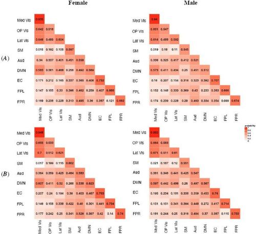
Fig. 2 MMM estimated probabilities of latent structural connection (SC) in different subject groups. Row (A) represents the younger group (Age 8–15) and Row (B) represents the older group (Age 16–21). The numeric value in each module block indicates the estimated probability and the color shade indicates the magnitude of the probability. Within-module SC is stronger compared with between-module SC. Modules with similar functionality, for example, Med Vis, OP Vis and Lat Vis, are found to have stronger SC.

To measure functional connectivity, we followed the procedure in Wang et al. (2016) by first detrending, demeaning, and whitening fMRI BOLD time series at each voxel. We extracted the representative fMRI BOLD series from each node by averaging the time series from all the voxels within the node. We then evaluated FC for each subject by calculating Pearson correlation between the representative time series extracted from the nodes. Fisher’s transformation was then applied to the correlation coefficients to obtain the final FC measures. We evaluated structural connections based on dMRI data from the PNC study. First, we followed the approach in Rudie et al. (2013) and dilated each node in Power’s system to 20mm diameter sphere to include white matter voxels for the nodes. To measure structural connectivity, we used the FSL functions “BEDPOSTX” and “PROBTRACKX2” to estimate the distribution of fiber orientations at each voxel and conducted the probabilistic tractography algorithm to estimate the count of white matter fibers tracts connecting pairs of brain regions. In the probabilistic tractography, fiber tracks passing through gray matter or cerebrospinal fluid were discarded. The SC for each node pair was then calculated based on the proportion of fiber tracts connecting the two node regions out of the total number of permissible tracts initiated at the node regions. A logit transformation was applied to obtain the final SC measures.

3.3 Results of the PNC Study

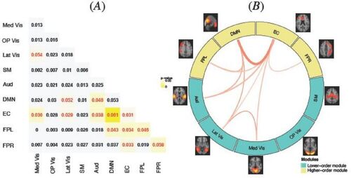
We applied the proposed MMM to jointly modeling the FC and SC measures in terms of gender and age group. We also investigated potential interactions between gender and age group in the MMM but didn’t identify significant interaction effects based on our data. Hence, the final MMM model included the main effects of gender and age. In Figure 2, we presented the model estimated structural connection probabilities for the four subject groups, that is, $\left\{{\widehat{\pi }}_{m(j)m(k),g}\right\}$. The general pattern of SC appeared to be similar across the groups where within-module SC tended to be stronger than between-module SC, indicating there is generally stronger structural connections between nodes that belong to the same functional module. This aligns with the significant role of white matter fiber tracts among brain regions that demonstrate coherent functional activities. In addition, the results showed that there was particularly strong structural connection among the three visual modules: Med Vis, OP Vis and Lat Vis, which are very close to each functionally and anatomically. This finding is consistent with previous findings of dense structural connectivity in visual cortex (Hagmann et al. 2008). Results from MMM allow us to investigate the neurodevelopmental related differences in SC across the networks. In Figure 3, we presented the estimated difference in structural connection probabilities between the older and younger age group for female. The results for male were similar and hence omitted here and later. Figure 3 showed a general increase in white fiber structural connections across the brain with the increase in age. In particular, we observed that the increase in white matter fiber connection was especially noticeable and more statistically significant for higher-order cognitive networks such as DMN, EC, FPL and FPR as compared to primary sensory and motor networks. Specifically, most of the significant increases were found in the fiber tracts connections within or between these higher-order cognitive networks and also in the fiber tracts connections between some of the cognitive networks and sensory networks, for example, between EC and auditory/visual networks. MMM revealed the most significant increase in SC is between DMN and EC where the probability of structural connection between them increases by about 15%. Previous work based on cortical thickness indicated early maturation of structural networks in primary sensorimotor regions in childhood while protracted development of higher-order cognitive regions happen later during adolescence (Khundrakpam et al. 2012). MMMs results in Figure 3 provide new findings from white fiber tracts connections that are consistent with the previous findings from cortical thickness, showing there is more significant increase in structural connections in high-order cognitive networks for older adolescents as compared to younger adolescents and children.

Fig. 3 MMM estimated difference in structural connection (SC) probabilities between the older (16–21) and younger (8–15) age group. (A): the numeric values are the estimated age difference (older vs. younger) in the SC probabilities. We highlight in yellow the age differences that are significant at the alpha = 0.05 level, where the color of the numeric values indicates the direction of the difference (red = significant positive difference; blue = significant negative difference). (B): A graphical illustration of the significant differences in SC across brain networks presented in (A). Turquoise modules represent higher-order cognitive networks and yellow modules represent lower-order modules such as primary sensory and motor networks. The red lines show significantly increased SC with age, with the wider lines representing more significant age difference with smaller p-values.

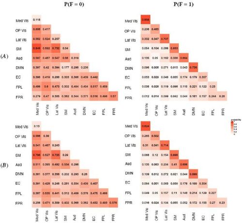
Figure 4 represents the estimated probability for the latent functional connectivity state for two subject groups: younger female and older female. For the tri-state functional connection, we presented the estimated probabilities for F = 0 and F = 1, corresponding to no connection and positive connection, respectively. The estimated probabilities for F = – 1 is presented in the supplementary materials because it is determined given the other two states and also because the understanding of negative correlations still remains elusive in neuroscience literature and research interests mainly focus on positive functional connections. Figure 4 showed overall pattern of FC appeared to be similar across the groups with some differences in certain modules. As the general FC pattern, the highest probability of having positive connections, that is, F = 1, were observed among within-module connections represented by the diagonal blocks in Figure 4. For between-module connections, the probability of positive FCs was generally higher between modules with similar type of functionality. For example, we observed higher probability of positive FCs among primary sensory and motor networks (e.g., Med Vis, Op Vis, Lat Vis, SM, Aud) and among higher-order cognitive networks (e.g., DMN, EC, FPL and FPR), while the probability of positive FC between the two types of networks is generally lower. Previous studies (Mesulam 1998) provided evidence primarily from brain activation analysis that the brain functionality can be grouped into primary sensory and motor functions (e.g., visual, auditory, motor) and higher-order cognition function (e.g., attention, emotion, memory, executive.). Our results contribute findings based on brain connectivity analysis to further support this paradigm and also provide new understanding on the connections between brain regions involved in these different functionalities.

Fig. 4 MMM estimated probabilities for the latent functional connectivity state for two subject groups: (A) younger female and (B) older female. The numeric value in each module block indicates the estimated probability and the color shade indicates the magnitude. The highest probability of having positive connections, that is, F= 1, were observed among within-module connections represented by the diagonal blocks. For between-module connections, the probability of positive FCs were generally higher between modules with similar type of functionality.

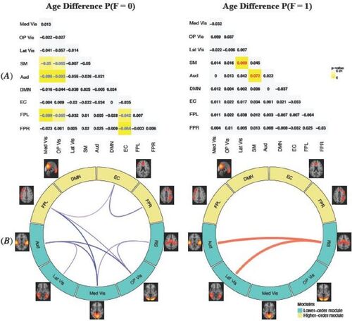
To investigate neurodevelopmental related differences in FC across the networks, we display the MMM estimated difference in functional connection probabilities between the older and younger age group for female (Figure 5). The results for male were similar and hence omitted here and later. As age increase from 8–15 to 16–21, the probability of the state of having no FC (F = 0) generally decreased across networks while the probability of positive FC (F = 1) mostly increased, indicating the brain becomes more functionally ordered or connected during adolescence. In particular, with the increase of age, we found a significant increase in the probability of positive FC between SM and Lat Vis and between SM and Aud, which is consistent with findings in the literature (Cai et al. 2018).

Fig. 5 MMM estimated difference in probabilities of functional connection state between the older (16–21) and younger (8–15) age group. (A): the estimated age difference (older vs. younger) for the probabilities of no FC (F = 0) and positive FC (F = 1). We highlight in yellow the age differences that are significant at the alpha = 0.05 level, where the color of the numerical values indicates the direction of the difference (red = significant positive difference; blue = significant negative difference). With age increases, the probability of no FC (F = 0) generally decreases across the networks and the probability of positive FC (F = 1) generally increases across the networks, indicating the brain gets more functionally organized with neurodevelopment. (B): A graphical illustration of the significant age differences in functional connections across brain networks presented in (A). Turquoise modules represent higher-order cognitive networks and yellow modules represent lower-order modules such as primary sensory and motor networks. The blue lines show probabilities that significantly decreases with age increase and the red lines show probabilities that significantly increases. Wider lines represent more significant age differences with smaller p-value.

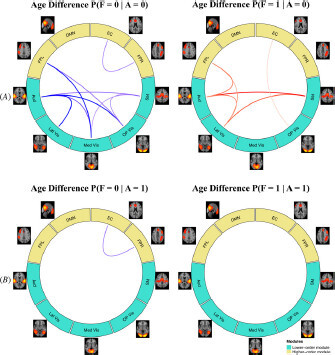
A research question that attracts considerable interests in neurodevelopment studies is whether the function connectivity changes with age differ across the brain between region pairs that have direct structural connections and those that don’t. With the joint modeling of the FC and SC, MMM provides a useful analytical tool to investigate this problem. We evaluated the change in FC with increase of age under the two different latent structural connection states (Figure 6). Consistent with the findings in our marginal analysis on FC change, we found that with age increases, the probability of no FC generally decreased across networks and the probability of positive FC generally increased across networks, regardless of the latent structural connection state. An interesting new finding from the conditional analysis based on the latent structure state was that most significant changes in FC were observed at those edges with latent structural state of A = 0 while very limited age differences in FC were found for edges with A = 1. Considering the age range of the age groups in the study, our findings suggest that functional connection development from late childhood and early adolescence to late adolescence mainly happen at edges that do not have strong direct structural connections. These are typically long-range edges and edges that are functionally integrated not by local structural connections but rather via the global brain hierarchical organization. Our finding aligns with some previous studies that showed the strengthening of long-range functional connections and functional integration across the brain happen from late childhood to adolescence and early adulthood due to brain maturity during this period (Ernst et al. 2015).

Fig. 6 MMM estimated age difference in probabilities of functional connection states conditional on the structural state. (A): significant age differences (older vs. younger) for no FC (F = 0) and positive FC (F = 1), conditioning on no SC (A = 0). (B): significant age differences for FC, conditioning on the presence of SC (A = 1).

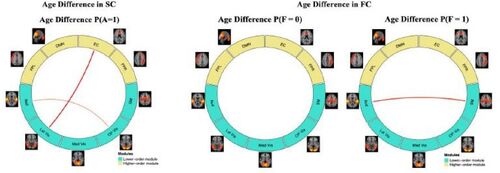
As a comparison to the MMM model, we considered an alternative method that models SC and FC separately and conducts edge-wise analysis to assess between group differences. Detailed information of the comparison model is presented in supplementary materials. Figure 7 illustrated the significant age differences found by the comparison model in the structural and functional connections. Compared to MMMs findings in Figures 3 and 5, the comparison model was only able to identify changes in the SC and FC between a very few brain modules. Unlike MMM, the comparison model failed to reveal the strengthening of brain structural and functional connections with neurodevelopment. Furthermore, since the comparison method models the SC and FC separately, it was unable to provide the insights on the functional connection development conditional on the presence of structural connections. These results show that MMM provides a more powerful tool to obtain neurobiologically meaningful insights in neurodevelop- ment.

Fig. 7 Estimated age differences in probabilities of structural and functional connection based on the comparison model.

4 Application to Simulated Data

We evaluated the performance of the proposed MMM and study the accuracy of estimation and inference procedure using simulated data. To mimic the real data, we considered the setting where there were four subgroups each with 50 subjects, two covariates and five brain functional modules. Number of nodes in each brain module was 15, 15, 19, 20, and 39, which were based on the module size of the visual networks, DMN and EC modules in the real data analysis. We generated two binary covariates corresponding to the age group and gender group. To specify the parameters in the latent structural connectivity state model, we chose a series of values for the ${\mathbf{\Theta }}_1=(\mathit{\beta },{\mathit{\alpha }}^{u,-1},{\mathit{\alpha }}^{u,1})$ parameters based on the range of their estimates from the PNC study. Similarly, we specified other parameters in the model based on their estimated value obtained from the PNC study, which are summarized in Table 2.

Table 2 Parameters of structural and functional measure in simulation.

Structural	State	u = 0			u = 1
	ρ	0.716			0.083
	γ	0.186	0.399	0.415	0.115	0.519	0.366
	χ	2.593	3.421	4.837	3.746	6.293	9.364
	${\xi }^2$	0.034	0.258	1.162	0.601	2.279	4.964
	State	u = 0			u = 1
		v = –1	v = 0	v = 1	v = –1	v = 0	v = 1
Functional	μ	−0.188	−0.006	0.252	−0.101	0.168	0.528
	${\sigma }^2$	0.073	0.078	0.105	0.083	0.097	0.132

We simulated functional connectivity and structural connectivity measurements for each subject based on the specified parameters. We first generated the latent structural state for each connection from the Bernoulli distribution and then simulated the latent functional state conditioned on latent structural state from a trinomial distribution. Next, structural connectivity and functional connectivity measurements for each connection were generated based on the latent structural and latent functional state following the observed SC and FC models in (1) and (2). We conducted 1000 Monte Carlo simulation runs and generated 200 parameteric bootstrap samples for each simulated dataset to obtain the bootstrap variance estimation.

Figure 8 presents the estimation results of the module-wise parameters ${\mathbf{\Theta }}_1=(\mathit{\beta },{\mathit{\alpha }}^{u,-1},{\mathit{\alpha }}^{u,1})$ which are of most interest in the study. Results showed the proposed method successfully estimated these parameters across the module blocks with high accuracy and very small bias. In addition, the proposed bootstrap variance estimation demonstrated good performance where the average bootstrap variance estimates across simulation runs for each parameter were very close to the Monte Carlo empirical variance. Detailed results are presented in Section 3 in the supplementary materials. Figure 9 displays the 95% confidence interval coverage probability for the covariate effects parameters. 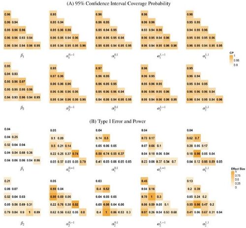It also presents Type I error and power for testing covariate effects hypothesis, for example, $H_0:{\beta }_1=0$ versus $H_1:{\beta }_1\ne 0$, at each module block given 0.05 significance level. We found that the coverage probability were close to 95% for most parameters. The Type I error at module blocks without covariate effects, that is, α or β parameter is zero, was generally close to the 5% nominal level. The statistical power for detecting nonzero covariate effects increased as the increase of the effect size as expected.

Fig. 8 Results for estimating covariate effects parameters in MMM. We present the true values and the estimates based on the average across 1000 simulation replicates.

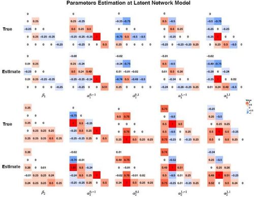
Fig. 9 Empirical coverage probabilities for the 95% confidence interval and statistical testing results for the covariate effects parameters. In (A), numeric values represent the empirical coverage probabilities of the 95% Confidence Interval. In (B), numeric values represent the empirical rejection rate in the hypothesis testing. Module blocks are colored according to their true covariate effect size where blocks without covariate effects, that is, with the parameter of 0, are shown as white. The rejection rate value represents Type I error for the white module blocks without covariate effects and represents statistical power for the colored module blocks with covariate effects.

5 Discussion

In this article, we present multimodal multilevel model (MMM) for jointly investigating brain networks using both functional and structural brain imaging modalities. It provides a tool to infer latent structural state, latent functional state and their inter-relationship based on noisy multimodal imaging observations. In addition, a formal statistical framework for modeling and testing group differences in brain networks is provided. The proposed module-specific latent network model allows investigation of heterogeneity in the connectivity states as well as covariate effects (i.e., neurodevelopment, disease-related, treatment-related) across different networks in the brain. Through simulation studies, we show that the proposed model can achieve accurate parameter estimation and valid inference. In addition, our analysis of the PNC study using the MMM brings new insights about the development of brain structural and functional connectivity during late childhood and adolescence. The computational complexity of the MMM is $O(I{Q}^2)$, where I is number of individuals and Q is number of nodes. The PNC analysis took 43 min on a 1.4 GHz Quad-Core Intel Core i5 processor with 8 GB RAM. Codes are be provided at our github site https://github.com/Emory-CBIS/MMM.

For MMM, we propose a module-wise parameterization based on brain network topology to achieve a balance between the computational efficiency and modeling precision in whole-brain connectomics. We adopt one of the most highly cited brain module system by Smith et al. (2009). Functional modules such as Smith’s system has a close correspondence with structural modules (Sporns and Betzel 2016). As a sensitivity analysis, we consider an alternative module system used in the Power’s node system paper (Power et al. 2011). We obtain similar findings as those based on Smith’s system. Please refer to Section 7 of supplementary materials for details.

The proposed MMM can be extended in multiple directions. For example, at the second level of MMM, the data generative models for the transformed FC and SC measures are specified based on the observed empirical distributions of these measures and are generally appropriate across different transformation functions. In practice, users can also check the validity of the form of the models based on the empirical distributions of the FC and SC measures in their studies. If needed, the data generative model for FC can be modified to accommodate non-Gaussianity, such as using the mixture of Gaussian. The EM algorithm can be modified to accommodate alternative data generative models. As another example of possible extensions, while MMMs FC data-generative model currently only accounts for direct SC via direct white fiber tract connections, MMM can be extended to accommodate indirect SC via intermediate nodes (Kang et al. 2017). For example, one can add an additional latent structural state for indirect SC and model the latent structure state variable A using the multinomial distribution. MMM can also be extended to model time-varying FC. Specifically, We can modify the FC data generative model to model time-varying FC measures in terms of time-varying latent functional states which can be modeled via a multinomial distribution with time-varying multinomial proportions. In the latent network modeling, the time-varying multinomial proportions can be modeled in terms of covariate via a Generalized Linear Mixed Model (Hedeker 2003) which accounts for the correlation among the proportions.

Supplementary Materials

The supplementary materials contains theoretical details, additional simulation results, empirical analysis results for the PNC study, analysis results from a different module system and from a comparison model.

Funding

The authors gratefully acknowledge support from NIH under award number R01MH105561, R01MH118771, R01EB027147, and R01MH119251. The content is solely the responsibility of the authors and does not necessarily represent the official views of the National Institutes of Health. Philadelphia Neurodevelopmental Cohort: Support for the collection of the data sets was provided by grant RC2MH089983 awarded to Raquel Gur and RC2MH089924 awarded to Hakon Hakorson. All subjects were recruited through the Center for Applied Genomics at The Children’s Hospital in Philadelphia.

References

- Albert, A., and Anderson, J. A. (1984), “On the Existence of Maximum Likelihood Estimates in Logistic Regression Models,” Biometrika, 71, 1–10. DOI: 10.1093/biomet/71.1.1.
- Behrens, T. E., Woolrich, M. W., Jenkinson, M., Johansen-Berg, H., Nunes, R. G., Clare, S., Matthews, P. M., Brady, J. M., and Smith, S. M. (2003), “Characterization and Propagation of Uncertainty in Diffusion-Weighted MR Imaging,” Magnetic Resonance in Medicine: An Official Journal of the International Society for Magnetic Resonance in Medicine, 50, 1077–1088. DOI: 10.1002/mrm.10609.
- Bressler, S. L., and Tognoli, E. (2006), “Operational Principles of Neurocognitive Networks,” International Journal of Psychophysiology, 60, 139–148. DOI: 10.1016/j.ijpsycho.2005.12.008.
- Bull, S. B., Mak, C., and Greenwood, C. M. (2002), “A Modified Score Function Estimator for Multinomial Logistic Regression in Small Samples,” Computational Statistics & Data Analysis, 39, 57–74.
- Cai, B., Zille, P., Stephen, J. M., Wilson, T. W., Calhoun, V. D., and Wang, Y. P. (2018), “Estimation of Dynamic Sparse Connectivity Patterns from Resting State fMRI,” IEEE Transactions on Medical Imaging, 37, 1224–1234. DOI: 10.1109/TMI.2017.2786553.
- Côté, M.-A., Girard, G., Boré, A., Garyfallidis, E., Houde, J.-C., and Descoteaux, M. (2013), “Tractometer: Towards Validation of Tractography Oipelines,” Medical Image Analysis, 17, 844–857. DOI: 10.1016/j.media.2013.03.009.
- Ernst, M., Torrisi, S., Balderston, N., Grillon, C., and Hale, E. A. (2015), “fMRI Functional Connectivity Applied to Adolescent Neurodevelopment,” Annual Review of Clinical Psychology, 11, 361–377. DOI: 10.1146/annurev-clinpsy-032814-112753.
- Firth, D. (1993), “Bias Reduction of Maximum Likelihood Estimates,” Biometrika, 80, 27–38. DOI: 10.1093/biomet/80.1.27.
- Hagmann, P., Cammoun, L., Gigandet, X., Meuli, R., Honey, C. J., Wedeen, V. J., and Sporns, O. (2008), “Mapping the Structural Core of Human Cerebral Cortex,” PloS Biology, 6, e159. DOI: 10.1371/journal.pbio.0060159.
- Hedeker, D. (2003), “A Mixed-Effects Multinomial Logistic Regression Model,” Statistics in Medicine, 22, 1433–1446. DOI: 10.1002/sim.1522.
- Henry, T. R., and Cohen, J. R. (2019), “Dysfunctional Brain Network Organization in Neurodevelopmental Disorders,” in Connectomics, eds. B. C. Munsell. G. Wu, L. Bonilha, and P. J. Laurienti, pp. 83–100, Amsterdam: Elsevier.
- Higgins, I. A., Kundu, S., and Guo, Y. (2018), “Integrative Bayesian Analysis of Brain Functional Networks Incorporating Anatomical Knowledge,” NeuroImage, 181, 263–278. DOI: 10.1016/j.neuroimage.2018.07.015.
- Hinne, M., Ambrogioni, L., Janssen, R. J., Heskes, T., and van Gerven, M. A. (2014), “Structurally-Informed Bayesian Connectivity Analysis,” NeuroImage, 86, 294–305. DOI: 10.1016/j.neuroimage.2013.09.075.
- Honey, C., Sporns, O., Cammoun, L., Gigandet, X., Thiran, J.-P., Meuli, R., and Hagmann, P. (2009), “Predicting Human Resting-State Functional Connectivity from Structural Connectivity,” Proceedings of the National Academy of Sciences, 106, 2035–2040. DOI: 10.1073/pnas.0811168106.
- Kang, H., Ombao, H., Fonnesbeck, C., Ding, Z., and Morgan, V. L. (2017), “A Bayesian Double Fusion Model for Resting-State Brain Connectivity Using Joint Functional and Structural Data,” Brain Connectivity, 7, 219–227. DOI: 10.1089/brain.2016.0447.
- Kemmer, P. B., Wang, Y., Bowman, F. D., Mayberg, H., and Guo, Y. (2018), “Evaluating the Strength of Structural Connectivity Underlying Brain Functional Networks,” Brain Connectivity, 8, 579–594. DOI: 10.1089/brain.2018.0615.
- Khundrakpam, B. S., Reid, A., Brauer, J., Carbonell, F., Lewis, J., Ameis, S., Karama, S., Lee, J., Chen, Z., Das, S., Evans, A. C., and Brain Development Cooperative Group. (2012), “Developmental Changes in Organization of Structural Brain Networks,” Cerebral Cortex, 23, 2072–2085. DOI: 10.1093/cercor/bhs187.
- Krogsrud, S. K., Fjell, A. M., Tamnes, C. K., Grydeland, H., Mork, L., Due-Tønnessen, P., Bjørnerud, A., Sampaio-Baptista, C., Andersson, J., Johansen-Berg, H., and Walhovd, K. B. (2016), “Changes in White Matter Microstructure in the Developing Brain—A Longitudinal Diffusion Tensor Imaging Study of Children from 4 to 11 Years of Age,” Neuroimage, 124, 473–486. DOI: 10.1016/j.neuroimage.2015.09.017.
- Liu, T. T. (2016), “Noise Contributions to the fMRI Signal: An Overview,” NeuroImage, 143, 141–151. DOI: 10.1016/j.neuroimage.2016.09.008.
- Louis, T. A. (1982), “Finding the Observed Information Matrix When Using the EM Algorithm,” Journal of the Royal Statistical Society, Series B, 44, 226–233.
- Mastrandrea, R., Gabrielli, A., Piras, F., Spalletta, G., Caldarelli, G., and Gili, T. (2017), “Organization and Hierarchy of the Human Functional Brain Network Lead to a Chain-like Core,” Scientific Reports, 7, 1–13. DOI: 10.1038/s41598-017-04716-3.
- Mesulam, M.-M. (1998), “From Sensation to Cognition,” Brain: A Journal of Neurology, 121, 1013–1052. DOI: 10.1093/brain/121.6.1013.
- Meunier, D., Lambiotte, R., and Bullmore, E. T. (2010), “Modular and Hierarchically Modular Organization of Brain Networks,” Frontiers in Neuroscience, 4, 200. DOI: 10.3389/fnins.2010.00200.
- Power, J. D., Cohen, A. L., Nelson, S. M., Wig, G. S., Barnes, K. A., Church, J. A., Vogel, A. C., Laumann, T. O., Miezin, F. M., Schlaggar, B. L., Petersen, S. E. (2011), “Functional Network Organization of the Human Brain,” Neuron, 72, 665–678. DOI: 10.1016/j.neuron.2011.09.006.
- Rubia, K., Overmeyer, S., Taylor, E., Brammer, M., Williams, S., Simmons, A., Andrew, C., and Bullmore, E. (2000), “Functional Frontalisation with Age: Mapping Neurodevelopmental Trajectories with fMRI,” Neuroscience & Biobehavioral Reviews, 24, 13–19.
- Rudie, J. D., Brown, J., Beck-Pancer, D., Hernandez, L., Dennis, E., Thompson, P., Bookheimer, S., and Dapretto, M. (2013), “Altered Functional and Structural Brain Network Organization in Autism,” NeuroImage: Clinical, 2, 79–94. DOI: 10.1016/j.nicl.2012.11.006.
- Satterthwaite, T. D., Wolf, D. H., Roalf, D. R., Ruparel, K., Erus, G., Vandekar, S., Gennatas, E. D., Elliott, M. A., Smith, A., Hakonarson, H., Verma, R., Davatzikos, C., Gur, R. E., and Gur, R. C. (2014), “Linked Sex Differences in Cognition and Functional Connectivity in Youth,” Cerebral Cortex, 25, 2383–2394. DOI: 10.1093/cercor/bhu036.
- Smith, S. M., Fox, P. T., Miller, K. L., Glahn, D. C., Fox, P. M., Mackay, C. E., Filippini, N., Watkins, K. E., Toro, R., Laird, A. R., and Beckmann, C. F. (2009), “Correspondence of the Brain’s Functional Architecture During Activation and Rest,” Proceedings of the National Academy of Sciences, 106, 13040–13045. DOI: 10.1073/pnas.0905267106.
- Sporns, O. (2013), “Structure and Function of Complex Brain Networks,” Dialogues in Clinical Neuroscience, 15, 247–262. DOI: 10.31887/DCNS.2013.15.3/osporns.
- Sporns, O., and Betzel, R. F. (2016), “Modular Brain Networks,” Annual Review of Psychology, 67, 613–640. DOI: 10.1146/annurev-psych-122414-033634.
- Van Der Vaart, A. W., and Wellner, J. A. (1996), “Weak Convergence,” in Weak Convergence and Empirical Processes, pp. 16–28, New York: Springer.
- Venkataraman, A., Rathi, Y., Kubicki, M., Westin, C.-F., and Golland, P. (2012), “Joint Modeling of Anatomical and Functional Connectivity for Population Studies,” IEEE Transactions on Medical Imaging, 31, 164–182. DOI: 10.1109/TMI.2011.2166083.
- Wang, Y., Kang, J., Kemmer, P. B., and Guo, Y. (2016), “An Efficient and Reliable Statistical Method for Estimating Functional Connectivity in Large Scale Brain Networks Using Partial Correlation,” Frontiers in Neuroscience, 10, 123. DOI: 10.3389/fnins.2016.00123.
- Williams, L. M. (2016), “Precision Psychiatry: A Neural Circuit Taxonomy for Depression and Anxiety,” The Lancet Psychiatry, 3, 472–480. DOI: 10.1016/S2215-0366(15)00579-9.
- Zalesky, A., Fornito, A., Cocchi, L., Gollo, L. L., van den Heuvel, M. P., and Breakspear, M. (2016), “Connectome Sensitivity or Specificity: Which is More Important?” Neuroimage, 142, 407–420. DOI: 10.1016/j.neuroimage.2016.06.035.
- Zhu, D., Zhang, T., Jiang, X., Hu, X., Chen, H., Yang, N., Lv, J., Han, J., Guo, L., and Liu, T. (2014), “Fusing DTI and fMRI Data: A Survey of Methods and Applications,” NeuroImage, 102, 184–191. DOI: 10.1016/j.neuroimage.2013.09.071.