Benign Overfitting and Noisy Features

Abstract

Modern machine learning models often exhibit the benign overfitting phenomenon, which has recently been characterized using the double descent curves. In addition to the classical U-shaped learning curve, the learning risk undergoes another descent as we increase the number of parameters beyond a certain threshold. In this article, we examine the conditions under which benign overfitting occurs in the random feature (RF) models, that is, in a two-layer neural network with fixed first layer weights. Adopting a novel view of random features, we show that benign overfitting emerges because of the noise residing in such features. The noise may already exist in the data and propagates to the features, or it may be added by the user to the features directly. Such noise plays an implicit yet crucial regularization role in the phenomenon. In addition, we derive the explicit tradeoff between the number of parameters and the prediction accuracy, and for the first time demonstrate that overparameterized model can achieve the optimal learning rate in the minimax sense. Finally, our results indicate that the learning risk for overparameterized models has multiple, instead of double descent behavior, which is empirically verified in recent works. Supplementary materials for this article are available online.

Keywords:

• Double descent
• Errors-in-variables
• Kernel methods
• Minimax learning rate
• Random feature models

1 Introduction

Conventional learning wisdom suggests that one should carefully balance between underfitting and overfitting by controlling the capacity of the function class employed (Friedman, Hastie, and Tibshirani 2001). For example, in supervised learning with training data ${\{(x_i,y_i)\}}_{i=1}^n$ drawn from a probability measure ρ defined on $\mathcal{X}\times \mathcal{Y}$, we learn a predictor f chosen from some hypothesis space $\mathcal{H}$: $$\mathcal{H}:=\left\{f(x)=\sum _{i=1}^s{\beta }_{i}z(x,w_i), \beta =[{\beta }_1,\dots ,{\beta }_s]\in {ℝ}^s\right\},$$where s represents the number of features in the model. z is some nonlinear function, and $w_1,\dots ,w_s$ are the parameters associated with z. In this setting, traditional learning theory states that one should control the capacity of $\mathcal{H}$ either explicitly (e.g., choosing the right quantity s) or implicitly (e.g., early stopping or regularization) in order to prevent overfitting and achieve small generalization error. However, this classical learning theory has been challenged in recent years. In kernel regression, it has been observed that the lowest prediction error often occurs when λ = 0 (see, e.g., Belkin, Ma, and Mandal 2018; Liang and Rakhlin 2020). In addition, as demonstrated in Zhang et al. (2016), state-of-the-art deep networks are often trained to the interpolation regime where estimators perfectly fit the training data (i.e., they fit perfectly even when the noises are present in the labels, which indicates overfitting), yet they still generalize well to new examples. This benign overfitting phenomenon is also observed by interpolating kernel machines and deep networks even in the presence of significant label noise. Finally, in a series of insightful papers (Belkin, Ma, and Mandal 2018; Belkin et al. 2019; Belkin, Hsu, and Xu 2019), it is pointed out that the prediction accuracy for interpolating models often exhibits the double descent behavior empirically. In this framework, when the model complexity is small, that is, s < n, we are in the classical learning regime. As s approaches n, the training risk converges to zero while the true risk grows very large. However, as soon as s passes the threshold of n, the true risk starts to decrease again. Empirically, it is also observed that the minimum true risk achieved as $s\to \infty$ is lower than the minimum risk achieved in the s < n regime.

In this article, we study the benign overfitting behavior under the noisy feature setting, that is, noise that may exist in the covariates x or in the features z(x, w). Classical learning assumes that the training data ${\{(x_i,y_i)\}}_{i=1}^n$ are iid samples from joint distribution ρ on which the true risk is also evaluated. The prediction function is estimated by applying learning algorithm to the observed x (the covariates) or z(x, w) (the features), where x and z(x, w) are assumed to have no noise. However, in practice, the covariates or the features will often be noisy. The noise may already exist in the data (e.g., due to imperfect measurement equipment), or it may be added by the user (as we will elaborate later). In this contribution, we show that such noise acts as an implicit regularizer and gives rise to the benign overfitting phenomenon. Bartlett et al. (2020) are the first to propose that noisy feature might lead to benign overfitting under the linear regression setting. They have shown that if both the feature noise and eigenvalues of the covariance operator exhibit exponential decay, benign overfitting is observed. In Bunea, Strimas-Mackey, and Wegkamp (2020), the feature noise is taken into account under the linear factor regression setting. They demonstrate that under appropriate conditions of the feature noise, the interpolation yields near-optimal prediction risk, provided that the features and the response are jointly low-dimensional. In contrast, we study the effect of the covariates noises under the more general nonlinear feature map setting. Through adopting a novel random feature model with features sampled via Gaussian process formalism, we are not only able to derive the near-optimal prediction performance of the interpolator with much more relaxed assumptions (as illustrated in Section 3), but also demonstrate that the interpolator can achieve optimal learning rate in the minimax sense.

In our framework, similar to the classical learning, we first transform the covariate x to a feature vector z(x, w) through a nonlinear random map z (parameterized by w), and then apply regression to the feature vector z(x, w). However, a key difference in our work is that we assume each feature vector z(x, w) to be corroded with some noise ξ. In practice, there are multiple scenarios where the feature will have noise ξ. For instance, the noise might already reside in the covariates x, that is, $x_{{\xi }_0}=x+{\xi }_0$, giving rise to a noisy feature. Alternatively, a noise term ξ could be added deliberately by the user to the feature map z(x, w). For example, in the neural network setting, once we apply the feature map z to the covariates x, a bias term is typically added on top of z(w, x), which can be treated as the noise term. Finally, in factor regression or principal component regression, z(x, w) is either assumed to have noise or it is estimated by some algorithm (such as principal component analysis), which produces noisy features. In order to consider a general framework and to simplify the notation, we will thereafter write the noisy feature as $z_{\xi }(x,w)=z(x,w)+\xi$, where z(x, w) is the true feature while ξ represents the noise attached to z(x, w). Regression is then performed on the noisy feature $z_{\xi }(x,w)$. In this setting, we are interested in how the presence of ξ will affect the generalization performance of the interpolating estimator. Specifically, we make the following contributions:

• Novel Construction of Random Feature. We first propose a novel representation of the random feature models based on Mercer’s decomposition and Karhunen-Loève expansion (see Section 3.1). This new understanding of the random features reduces the nonlinear learning problem into a linear regression in the random feature space, and allows us to study the eigenspectrum of the sample covariance matrix, which is the key in analyzing the generalization properties of the interpolator. We also provide a detailed tradeoff between computational cost and prediction accuracy of the new random feature in Theorem 1;

• Implicit Regularization of Feature Noise. By assuming ξ to follow a normal distribution, Theorem 2 establishes a precise relationship between ξ and the excess learning risk. This characterization explains how ξ can act as an implicit regularization and prevent the explosion of the excess learning risk in the overparameterized setting. We remark that when considering linear regression where ρ has sub-Gaussian distribution, recent works by Bartlett et al. (2020) and Bunea, Strimas-Mackey, and Wegkamp (2020) provide alternatives to our bound in Theorem 2. However, our results apply to a more general nonlinear regression setting with many relaxed assumptions regarding the data generating distribution and the eigenspectrum of the covariance operator (see Section 3 for more details);

• Minimax Optimal Estimator. Our finite sample analysis reveals the detailed tradeoff between the number of parameters s and the prediction accuracy represented by the excess learning risk convergence rate. Moreover, under appropriate conditions, we show that the interpolator can achieve the optimal learning rate in the minimax sense;

• Multiple Descent Behavior. In Corollary 1, we extend our analysis of the excess learning risk to the case where ξ follows a sub-Gaussian distribution. Our results demonstrate that benign overfitting will occur as long as ξ decays with s at a prescribed rate, while the shape of the distribution is not a key component in driving the benign overfitting phenomenon. In addition, we analyze the behavior of the excess learning risk bound from Corollary 1 and explicitly show that incorporating feature noise into consideration leads to multiple descent of the learning risk. In particular, if the number of parameter s is beyond the $O(n^2)$ order, the learning risk starts to increase again, complementing the current findings of the double descent phenomenon. Our results are empirically verified in recent works by Adlam and Pennington (2020) and Liang, Rakhlin, and Zhai (2020).

Borrowing from the insight of Mercer’s decomposition and Karhunen-Loève expansion, we provide a detailed analysis of the generalization properties of the interpolator. All of our results apply to both the finite sample and the asymptotic case. They are also valid for data of arbitrary dimension. In addition, our results only impose very weak conditions on the kernel structure, that is, as long as its corresponding covariance operator is of trace class (see Assumption A.1). This is fundamentally different from the existing analysis of nonlinear feature map (Mei and Montanari 2019; Liao, Couillet, and Mahoney 2020), which only work for the Gaussian kernel. More importantly, our results have no specific assumption regarding the data generation distribution, which is a significant improvement on existing works (Mei and Montanari 2019; Bartlett et al. 2020; Bunea, Strimas-Mackey, and Wegkamp 2020), as they often assume the Gaussian or sub-Gaussian data generating distribution.

1.1 Related Work

The benign overfitting phenomenon of the interpolating estimator has drawn much interest in the machine learning community recently. For example Liang and Rakhlin (2020) derive the learning risk of the interpolating estimator in kernel ridgeless regression. They show that with certain properties of the kernel matrix and training data, there is an implicit regularization coming from the curvature of the kernel function. A follow-up work (Liang, Rakhlin, and Zhai 2020) further demonstrates that in very high dimension, kernel interpolator exhibits the multiple descent phenomenon. Belkin et al. (2019) experimentally demonstrate the double descent curve in both linear and nonlinear regression cases, and Belkin, Hsu, and Xu (2019) subsequently provide a finite sample analysis of the excess risk for the interpolating estimator in some special settings (where it is assumed that the responses and features are jointly Gaussian). By appealing to random matrix theory, Hastie et al. (2019) obtain the asymptotic behavior of the prediction accuracy in the linear regression setting with correlated features, where sample size n and the covariate dimension d both approach infinity with asymptotic ratio $d/n\to \gamma \in (0,\infty )$. They also study the asymptotic behavior of the variance term in the random nonlinear feature regression setting. Recently, by letting n, d and s all grow to infinity such that d/n and n/s remain bounded, Mei and Montanari (2019) derive the double descent curve in the random feature regression setting and obtain the asymptotic behavior. Later, Liao, Couillet, and Mahoney (2020) further extend the analysis of Mei and Montanari (2019) by relaxing the Gaussian assumptions on the data distribution while holding all other settings the same. A similar asymptotic behavior of the excess learning risk is obtained and the precise characterization of double descent is demonstrated. Finally, in a work that is most related to ours, Bartlett et al. (2020) study the upper and lower bound on the excess risk by assuming that the covariates belong to an infinite-dimensional Hilbert space and follow a sub-Gaussian distribution. Through investigating the finite sample learning risk behavior, they explicitly list the conditions for the overfitted linear model to have near-optimal prediction accuracy. Intuitively, for infinite dimensional covariates, the covariance operator spectrum has to decay slowly enough so that the sum of the tail of its eigenvalues is large compared to n. While for finite dimensional covariates, exponential decay for both the eigenspectrum of the covariance operator and the noise attached to the covariates is sufficient to guarantee the consistency of the interpolator.

2 Definitions and Notation

2.1 Regularized ERM and Kernel Learning

Let $\mathbf{x}$ and $\mathbf{y}$ be random variables with joint probability distribution $\rho (x,y)={\rho }_{\mathbf{x}}(x){\rho }_{\mathbf{y}}(y|x)$. In this article, we consider the regression problem where covariate $x\in \mathcal{X}\subset {ℝ}^d$ and response variable $y\in ℝ$. In addition, we will use the squared loss $l(y,f(x))={(y-f(x))}^2$ as the loss function.

In the regularized ERM with the squared loss, the optimal estimating regression function is $$f_{*}(x)=\mathbb{E}(\mathbf{y}|\mathbf{x}=x).$$

Let $X={[x_1,\dots ,x_n]}^T$ and $Y={[y_1,\dots ,y_n]}^T$ denote the training inputs and outputs. Given the function $\widehat{f}$ which is estimated based on (X, Y), we will consider the notion of excess risk as a measure of its generalization performance (Caponnetto and De Vito 2007) $$R_X(\widehat{f})={\mathbb{E}}_{\mathbf{x}}{\mathbb{E}}_{Y|X}\left[{(\widehat{f}(\mathbf{x})-f_{*}(\mathbf{x}))}^2|X\right].$$

Note that the excess risk is conditional on the training inputs X as emphasized by our notation R_X. However, when the context is clear, we will drop the subscript X for brevity.

The following kernel ridge regression (KRR) is an important class of ERM problems

Definition 1.

Given training example ${\{(x_i,y_i)\}}_{i=1}^n$ from ρ, a kernel function $K(·,·):\mathcal{X}\times \mathcal{X}\to ℝ$, and its corresponding reproducing kernel Hilbert space (RKHS) $\mathcal{H}$, the KRR problem is (1) $${\widehat{f}}^{\lambda }:=\text{arg}\hspace{0.17em}{\text{min}}_{f\in \mathcal{H}}\hspace{0.17em}\frac{1}{n}\sum _{i=1}^n(y_i-f(x_i){)}^2+\lambda |\left|f\right|{|}_{\mathcal{H}}^2.$$(1)

Here, λ is the regularization parameter and $\left|\right|·|{|}_{\mathcal{H}}$ represents the RKHS norm. Applying the representer theorem (Steinwart and Christmann 2008, Theorem 5.5), the solution to Equation (1)(1) $${\widehat{f}}^{\lambda }:=\text{arg}\hspace{0.17em}{\text{min}}_{f\in \mathcal{H}}\hspace{0.17em}\frac{1}{n}\sum _{i=1}^n(y_i-f(x_i){)}^2+\lambda |\left|f\right|{|}_{\mathcal{H}}^2.$$(1) can be written as $\widehat{f}(x)=K(x,X){(\mathbf{K}+n\lambda I)}^{-1}Y$, where $K(x,X)={[K(x,x_1),\dots ,K(x,x_n)]}^T$ and ${\mathbf{K}}_{i,j}=K(x_i,x_j)$ is the Gram matrix.

Random Fourier Features

Typically, kernel learning suffers from huge computation costs. Random Fourier features approximation (Rahimi and Recht 2007) is proposed to alleviate this problem. Specifically, if kernel K is translation invariant $K(x,y)=K(x-y)$, based on Bochner’s Theorem Bochner (1932), it can be written as $$K(x,y)=\int \left(\hspace{0.17em}\text{cos}\hspace{0.17em}(w^{T}x)+b\right)\left(\hspace{0.17em}\text{cos}\hspace{0.17em}(w^{T}y)+b\right)p(b)p(w)\mathit{dbdw},$$where $p(b),p(w)$ are certain probability distributions. As a result, if we sample $b_1,\dots ,b_s\sim p(v)$ and $w_1,\dots ,w_s\sim p(w)$, we can approximate the kernel as $$K(x,y)\approx \frac{1}{s}\sum _{i=1}^s\left(\hspace{0.17em}\text{cos}\hspace{0.17em}(w_i^{T}x)+b_i\right)\left(\hspace{0.17em}\text{cos}\hspace{0.17em}(w_i^{T}y)+b_i\right):={\tilde{\mathbf{z}}}_x^T{\tilde{\mathbf{z}}}_y.$$

We now let $\left|\right|A\left|\right|$ be the L₂ norm if A is a vector, or the operator norm if A is an operator. Since ${\tilde{\mathbf{z}}}_x$ is a random feature vector approximating the kernel k, we use these features to perform standard (linear) ridge regression on these features.

Definition 2.

Given ${\{({\tilde{\mathbf{z}}}_{x_i},y_i)\}}_{i=1}^n$ and corresponding feature matrix $\tilde{\mathbf{Z}}={[{\tilde{\mathbf{z}}}_{x_1},\dots ,{\tilde{\mathbf{z}}}_{x_n}]}^T\in {ℝ}^{n\times s}$, the random feature regression is (2) $${\beta }_{\lambda }:=\text{arg}\hspace{0.17em}{\text{min}}_{\beta \in {ℝ}^s} \frac{1}{n}\left|\right|Y-\tilde{\mathbf{Z}}\beta |{|}^2+\lambda s||\beta |{|}^2.$$(2)

Informally, we can see that instead of using functions in $\mathcal{H}$, random Fourier feature approximation employs functions in the RKHS spanned by the feature matrix $\tilde{\mathbf{Z}}$ to perform learning. As discussed before, we will mainly focus on the interpolator that perfectly fits the training data in this article. However, because there are infinitely many estimators as such, we will be working with the one that has the minimum norm defined as following

Definition 3.

Given feature vectors and response variables ${\{({\tilde{\mathbf{z}}}_{x_i},y_i)\}}_{i=1}^n$, we define the minimum norm least squares (MNLS) estimator as $$\underset{{}_{\beta \in {ℝ}^s}}{\min }\left|\right|\beta |{|}^2, \text{such} \text{that} ||\tilde{\mathbf{Z}}\beta -Y|{|}^2=\underset{{}_{{\beta }_0}}{\min }\left|\right|\tilde{\mathbf{Z}}{\beta }_0-Y|{|}^2.$$

By the projection theorem, the closed-form solution of the MNLS estimator is (3) $$\tilde{\beta }=\tilde{\mathbf{Z}}{(\tilde{\mathbf{Z}}{\tilde{\mathbf{Z}}}^T)}^{†}Y={({\tilde{\mathbf{Z}}}^T\tilde{\mathbf{Z}})}^{†}{\tilde{\mathbf{Z}}}^{T}Y,$$(3) where $A^{†}$ denotes the pseudoinverse for matrix A.

Remark 1.

We remark that in analyzing the generalization properties of the random Fourier feature interpolator $\tilde{\beta }$, a key issue is that the random variables $w_1,\dots ,w_s$ are embedded in the nonlinear feature map $\text{cos}\hspace{0.17em}(·)$. This nonlinear feature embedding makes the analysis of the eigenspectrum of ${\tilde{\mathbf{Z}}}^T\tilde{\mathbf{Z}}$ significantly hard. In light of this, we propose a novel way to construct random features in Section 3.1 to overcome this issue.

2.2 Bias-Variance Decomposition

The analysis of the excess learning risk often starts with the bias-variance decomposition. Hence, we present the bias-variance decomposition and introduce some relevant notations here to ease our following discussion. The following lemma gives the bias-variance decomposition. Its proof in Appendix B.1, supplementary materials is a simple nonlinear extension of the one in Hastie et al. (2019). Note that instead of working with $\tilde{\mathbf{Z}}$, we will use a different feature matrix in the rest of the article. As a result, we state the following bias-variance decomposition with an arbitrary feature matrix Z.

Lemma 1.

Let $\tilde{\beta }$ be the MNLS estimator as defined in Equation (3)(3) $$\tilde{\beta }=\tilde{\mathbf{Z}}{(\tilde{\mathbf{Z}}{\tilde{\mathbf{Z}}}^T)}^{†}Y={({\tilde{\mathbf{Z}}}^T\tilde{\mathbf{Z}})}^{†}{\tilde{\mathbf{Z}}}^{T}Y,$$(3) with feature matrix Z. Let $\tilde{f}(x)={\mathbf{z}}_x{(\mathbf{W})}^T\tilde{\beta }$ be the prediction from the MNLS estimator at a test point x. Define $\tilde{\mathcal{H}}$ as the RKHS spanned by the feature matrix Z and $f_{\tilde{\mathcal{H}}}$ as the best estimator such that $f_{\tilde{\mathcal{H}}}:=\text{arg}\hspace{0.17em}{\text{min}}_{f\in \tilde{\mathcal{H}}}{\mathbb{E}}_{\rho }{(f(x)-y)}^2$. Since $f_{\tilde{\mathcal{H}}}\in \tilde{\mathcal{H}}$, we let $f_{\tilde{\mathcal{H}}}(x)={\mathbf{z}}_x{(\mathbf{W})}^T{\beta }_{\tilde{\mathcal{H}}}$ for some ${\beta }_{\tilde{\mathcal{H}}}\in {ℝ}^s$. Define the bias and the variance as $$\begin{array}{c}{\mathbf{B}}_R:={\mathbb{E}}_{\mathbf{x}}\left[{\left({\mathbb{E}}_{Y|X}[\tilde{f}(\mathbf{x})]-f_{\tilde{\mathcal{H}}}(\mathbf{x})\right)}^2\right]={\mathbb{E}}_{\mathbf{x}}{\Vert {\mathbf{z}}_{\mathbf{x}}{(\mathbf{W})}^T\Pi {\beta }_{\tilde{\mathcal{H}}}\Vert }^2,\\ {\mathbf{V}}_R:={\mathbb{E}}_{\mathbf{x}}{ \text{var}}_{Y|X}(\tilde{f}(\mathbf{x})),\\ ={\mathbb{E}}_{\mathbf{x}}\left\{{\mathbb{E}}_{Y|X}{\Vert {\mathbf{z}}_{\mathbf{x}}{(\mathbf{W})}^T{({\mathbf{Z}}^T\mathbf{Z})}^{†}{\mathbf{Z}}^T(Y-f_{\tilde{\mathcal{H}}}(X))\Vert }^2\right\},\end{array}$$

where $f_{\tilde{\mathcal{H}}}(X)={[f_{\tilde{\mathcal{H}}}(x_1),\dots ,f_{\tilde{\mathcal{H}}}(x_n)]}^T$. In addition, we define the misspecification as $$\begin{array}{c}{\mathbf{M}}_R:={\mathbb{E}}_x{\left\{{\mathbf{z}}_x{(\mathbf{w})}^T{({\mathbf{Z}}^T\mathbf{Z})}^{†}{\mathbf{Z}}^T\left(f_{*}(X)-f_{\tilde{\mathcal{H}}}(X)\right)\right\}}^2\\ \hspace{1em}+{\mathbb{E}}_x{\left(f_{*}(x)-f_{\tilde{\mathcal{H}}}(x)\right)}^2.\end{array}$$

Then the following decomposition of the excess risk of $\tilde{\beta }$ holds $$R(\tilde{\beta })\le 3({\mathbf{M}}_R+{\mathbf{B}}_R+{\mathbf{V}}_R).$$

We can see that the excess learning risk is comprised of the bias ${\mathbf{B}}_R$, the variance ${\mathbf{V}}_R$ and the misspecification error ${\mathbf{M}}_R$. While we do not have a thorough understanding on how ${\mathbf{M}}_R$ evolves with the number of parameters s, we can reasonably assume that ${\mathbf{M}}_R$ decreases as we increase s. In addition, even in the classical regime where s < n, we observe that ${\mathbf{M}}_R\ll {\mathbf{V}}_R+{\mathbf{B}}_R$. As a result, in the interpolation regime where $s\gg n$, it is safe to assume that ${\mathbf{M}}_R\ll {\mathbf{V}}_R+{\mathbf{B}}_R$. In other words, the evolution of the excess learning risk is dominated by ${\mathbf{V}}_R$ and ${\mathbf{B}}_R$. Therefore, in the interpolating regime, our following analysis will mainly focus on ${\mathbf{B}}_R$ and ${\mathbf{V}}_R$ under the assumption that ${\mathbf{M}}_R=0$. In other words, we have ${\beta }_{*}={\beta }_{\tilde{\mathcal{H}}}$.

3 Main Results

3.1 Warm Up: Random Feature Approximation

Traditionally, random Fourier features approximation is a simple way to construct a finite-dimensional approximation of an infinite-dimensional kernel introduced by (Rahimi and Recht 2007). However, in this article, we propose a new way of constructing random feature approximation based on Mercer’s decomposition and Karhunen-Loève expansion. This novel construction can separate the random feature from the nonlinear feature map and hence reduce the nonlinear feature regression to a linear one. To the best of our knowledge, this novel perspective on random feature approximation is new to the literature.

Suppose that we consider kernel regression learning with a continuous kernel $K(·,·):\mathcal{X}\times \mathcal{X}\to ℝ$. By Mercer’s Theorem (Steinwart and Christmann 2008), we have (4) $$K(x,y)=\sum _{i=1}^P{\lambda }_i{e}_i(x)e_i(y),$$(4) where ${({\lambda }_i,e_i)}_{i=1}^P$ is the eigensystem corresponding to Mercer’s decomposition. ${\left\{e_i\right\}}_{i=1}^P$ is an at most countable orthonormal set of $L_2(d\rho )$ and ${\left\{{\lambda }_i\right\}}_{i=1}^P$ is a sequence of nonincreasing strictly positive eigenvalues. Based on Mercer’s decomposition, we have Karhunen-Loève expansion theorem (Kanagawa et al. 2018, Theorem 4.3) (also see (Steinwart 2019, Lemmas 3.3 and 3.7)) for Gaussian Process with kernel K.

Lemma 2

(Karhunen-Loève Expansion (Kanagawa et al. 2018, Theorem 4.3)). Let $K:\mathcal{X}\times \mathcal{X}\to ℝ$ be a continuous kernel, ν be a finite Borel measure with support on $\mathcal{X},$ and ${\left(e_i,{\lambda }_i\right)}_{i\in P}$ be that defined in Equation (4)(4) $$K(x,y)=\sum _{i=1}^P{\lambda }_i{e}_i(x)e_i(y),$$(4) . For a Gaussian process $f_K\sim \mathcal{G}\mathcal{P}(0,K)$, define $$w_i:={\lambda }_i^{-1/2}\int f(x)e_i(x)d\nu (x),\hspace{1em}i\in P.$$

Then the following are true

1. We have $$w_i\sim \mathcal{N}(0,1)\hspace{1em} \text{and} \hspace{1em}\mathbb{E}\left[w_i{w}_j\right]={\delta }_{ij},\hspace{1em}i,j\in P;$$

2. For all $x\in \mathcal{X}$ and for all finite $J\subset P,$ we have $$\mathbb{E}\left[{\left(f_K(x)-\sum _{j\in J}{w}_j{\lambda }_i^{1/2}{e}_j(x)\right)}^2\right]=k(x,x)-\sum _{j\in J}{\lambda }_j{e}_j^2(x);$$

3. If $P=\mathbb{N}$, we have $$\underset{n\to \infty }{\lim }\mathbb{E}\left[{\left(f_K(x)-\sum _{i=1}^n{w}_i{\lambda }_i^{1/2}{e}_i(x)\right)}^2\right]=0,\hspace{1em}x\in \mathcal{X},$$where the convergence is uniform in $x\in \mathcal{X}$.

Based on Karhunen-Loève expansion and denote w_i’s as iid $\sim \mathcal{N}(0,1)$, we can see that a Gaussian process $f_K\sim \mathcal{G}\mathcal{P}(0,K)$ has the expansion as $$f_K(x)=\sum _{i=1}^P{\lambda }_i^{1/2}{e}_i(x)w_i.$$

Since kernel K can be infinite-dimensional, that is, $P=\infty$, to ease the discussion, we will define a low-rank kernel k that approximates K by only using the top p < P eigenvalues and eigenvectors of Mercer’s decomposition in our analysis, that is, $$k(x,y)=\sum _{i=1}^p{\lambda }_i{e}_i(x)e_i(y):=V{(x)}^{T}DV(y),$$where we denote $V(x)={[e_1(x),\dots ,e_p(x)]}^T$ and $D=[{\lambda }_1,\dots ,{\lambda }_p]$.

Now for GP $f\sim \mathcal{G}\mathcal{P}(0,k)$, we can express it using Karhunen-Loève expansion $$f=V^T{D}^{1/2}\mathbf{w},$$where $\mathbf{w}$ is a p-dimensional Gaussian random vector with each entry being a standard normal random variable. From now on, we will use kernel k, and whenever we need to refer to K, we will treat K as the limit of k when $p\to P$.

If we sample ${\left\{{\mathbf{w}}^{(i)}\right\}}_{i=1}^s$ iid $\sim \mathbf{w}$, and let $z({\mathbf{w}}^{(i)},·)=V^T{D}^{1/2}{\mathbf{w}}^{(i)}$, ${\{z({\mathbf{w}}^{(i)},·)\}}_{i=1}^s$ are iid sample paths $\sim \mathcal{G}\mathcal{P}(0,k)$, such that ${\mathbb{E}}_{\mathbf{w}}(z({\mathbf{w}}^{(i)},x))=0$ and $${\mathbb{E}}_{\mathbf{w}}(z({\mathbf{w}}^{(i)},x)z({\mathbf{w}}^{(i)},y))=k(x,y).$$

In other words, we use $z({\mathbf{w}}^{(i)},·)$ as the random feature and approximate the kernel as $$k(x,y)\approx \frac{1}{s}\sum _{i=1}^{s}z({\mathbf{w}}^{(i)},x)z({\mathbf{w}}^{(i)},y).$$

In addition, we let $$\begin{array}{c}{\mathbf{z}}_x(\mathbf{W})=\frac{1}{\sqrt{s}}{\mathbf{W}}^T{D}^{1/2}V(x),\\ \mathbf{Z}={[{\mathbf{z}}_{x_1}(\mathbf{W}),\dots ,{\mathbf{z}}_{x_n}(\mathbf{W})]}^T=\frac{1}{\sqrt{s}}V(X)D^{1/2}\mathbf{W},\end{array}$$where $$\begin{array}{c}\mathbf{W}=[{\mathbf{w}}^{(1)},\dots ,{\mathbf{w}}^{(s)}]\in {ℝ}^{p\times s},\\ V(X)={[V(x_1),\dots ,V(x_n)]}^T\in {ℝ}^{n\times p}.\end{array}$$

It is easy to verify that $k(x,y)={\mathbb{E}}_{\mathbf{w}}[{\mathbf{z}}_x{(\mathbf{W})}^T{\mathbf{z}}_y(\mathbf{W})]$ and $\mathbf{K}={\mathbb{E}}_{\mathbf{w}}(\mathbf{Z}{\mathbf{Z}}^T)$. In addition, the MNLS estimator under the new random feature model is similar to Equation (3)(3) $$\tilde{\beta }=\tilde{\mathbf{Z}}{(\tilde{\mathbf{Z}}{\tilde{\mathbf{Z}}}^T)}^{†}Y={({\tilde{\mathbf{Z}}}^T\tilde{\mathbf{Z}})}^{†}{\tilde{\mathbf{Z}}}^{T}Y,$$(3) and has the following form $$\tilde{\beta }={({\mathbf{Z}}^T\mathbf{Z})}^{†}{\mathbf{Z}}^{T}Y.$$

Covariance Operator

Based on the new random feature, we define the following various forms of covariance operator

• Let Σ be the population covariance operator of kernel k with eigenvalue matrix D $$\Sigma ={\mathbb{E}}_{\mathbf{x}}\left\{D^{1/2}V(\mathbf{x})V{(\mathbf{x})}^T{D}^{1/2}\right\};$$

• Let $\widehat{\Sigma }$ be the sample estimate of Σ and $\widehat{D}= \text{diag}({\widehat{\lambda }}_1,\dots ,{\widehat{\lambda }}_n)$ be its eigenvalue matrix; $$\widehat{\Sigma }=\frac{1}{n}\sum _{i=1}^n{D}^{\frac{1}{2}}V(x_i)V{(x_i)}^T{D}^{\frac{1}{2}}.$$

• Let ${\widehat{\Sigma }}^s$ be the random feature approximation of $\widehat{\Sigma }$ with s features $${\widehat{\Sigma }}^s=\frac{1}{n}{\mathbf{Z}}^T\mathbf{Z}.$$

The eigenvalue matrix is denoted to be ${\widehat{D}}^s= \text{diag}({\widehat{\lambda }}_1^s,\dots ,{\widehat{\lambda }}_N^s)$.

3.1.1 Generalization Property

Recently, there has been a large research interest in understanding the efficiency of the random Fourier feature ${\tilde{\mathbf{z}}}_x$ introduced in Section 2.1 (see, e.g., Bach 2017; Avron et al. 2017; Rudi and Rosasco 2017; Li et al. 2019). In particular, a detailed tradeoff between computational cost and prediction accuracy is thoroughly investigated in the regression setting, that is, Definition 2. These results show that $\Omega (\sqrt{n}\hspace{0.17em}\text{log}\hspace{0.17em}n)$ random Fourier features can guarantee the minimax optimal $O(1/\sqrt{n})$ learning rate, which reduces the computational cost and memory from $O(n^3)$ and $O(n^2)$ to $O(n^2)$ and $O\left(n\sqrt{n}\right)$. Hence, one might be interested in whether the new constructed random feature can achieve a similar computational savings. Theorem 1 provides a definitive answer.

Theorem 1.

Suppose we perform ridge random feature regression with regularization parameter λ and the new feature by replacing $\tilde{\mathbf{Z}}$ with Z in Equation (2)(2) $${\beta }_{\lambda }:=\text{arg}\hspace{0.17em}{\text{min}}_{\beta \in {ℝ}^s} \frac{1}{n}\left|\right|Y-\tilde{\mathbf{Z}}\beta |{|}^2+\lambda s||\beta |{|}^2.$$(2) . Let the random feature regression estimator to be ${\tilde{f}}_z$ and recall our original kernel is K with its RKHS $\mathcal{H}$. Denote $\mathbb{E}(l_f)=\mathbb{E}{(f(x)-y)}^2$ and $f_{\mathcal{H}}:=\text{arg}\hspace{0.17em}{\text{min}}_{f\in \mathcal{H}}\mathbb{E}(l_f)$. In addition, for kernel K with Gram-matrix K, we denote $d_{\mathbf{K}}^{\lambda }= \text{Tr}(\mathbf{K}{(\mathbf{K}+n\lambda I)}^{-1})$. For any $\delta \in (0,1)$ and some parameter λ and η depend only on n, if $$p\ge \frac{c_1}{\eta }\text{log}\hspace{0.17em}\frac{d_{\mathbf{K}}^{\lambda }}{\delta }, \& s\ge \frac{1}{\lambda }\text{log}\hspace{0.17em}\frac{d_{\mathbf{K}}^{\lambda }}{\delta },$$

we have (5) $$\mathbb{E}(l_{{\tilde{f}}_z})-\mathbb{E}(l_{f_{\mathcal{H}}})\le \lambda +\eta +O(1/\sqrt{n}).$$(5)

Theorem 1 shows that using the new random feature can indeed provide us computational gain without sacrificing the prediction accuracy in ridge regression. To see this, we first note that for kernel ridge regression, the computational cost and the memory is $O(n^3)$ and $O(n^2)$, respectively, and the minimax optimal learning rate is $O(1/\sqrt{n})$ (Caponnetto and De Vito 2007). On the other hand, regression with our constructed random feature requires $O(n{s}^2+s^3)$ in time and O(ns) in memory. Hence, to what extend can random feature regression provide computational gain depends on the choice of s. Theorem 1 states that the excess risk learning rate of $O(1/\sqrt{n})$ can be achieved if we let $\lambda =O(1/\sqrt{n})$ and $\eta =O(1/\sqrt{n})$. Under this setting, we can see that $p=O\left(\sqrt{n}\right)$ and $s=O\left(\sqrt{n}\right)$ ² . In other words, we obtain the same learning rate as kernel ridge regression while the computational cost and the memory is reduced to $O(n^2)$ and $O(n^{1.5})$. In addition, Theorem 1 provides a detailed tradeoff between computational cost and prediction accuracy. For example, if we are willing to decrease the prediction accuracy to $O(n^{-1/3})$ by letting $\lambda =O(n^{-1/3})$ and $\eta =O(n^{-1/3})$, we can see that the random feature regression only requires $O(n^{5/3})$ in time and $O(n^{4/3})$ in memory.

Remark 2.

Theorem 1 mainly considers the worst-case scenario where the regression estimator achieves the minimax optimal learning rate $O(1/\sqrt{n})$. However, we remark that a similar tradeoff in the fast learning rate case can be easily obtained via using the local Rademacher complexity technique (Bartlett, Bousquet, and Mendelson 2005). Moreover, the computational requirement can be further reduced to even a constant number of features. Nevertheless, we skip the results since our major focus is to understand the benign overfitting phenomenon. Interested readers can refer to Rudi and Rosasco (2017) and Li et al. (2021) for the refined analysis in the fast learning rate setting.

3.2 Benign Overfitting with Noisy Random Features

In this section, we discuss how the behavior of the excess learning risk of the MNLS estimator is affected by the noise in the features. We demonstrate how the new evolution of the excess learning risk leads to benign overfitting and, in particular, to the double descent phenomenon. In the following discussion, we let $P>p>n,s$ without loss of generality. In addition, since we are mainly interested in the overparameterized regime, we let $s\ge n$.

As discussed, we consider the noisy feature setting: $z_{\xi }(x,w)=z(x,w)+\xi$. We denote the s-dimensional noisy feature as ${\mathbf{z}}_x^{\xi }(\mathbf{W})={\mathbf{z}}_x(\mathbf{W})+\mathit{\xi }$, where $\mathit{\xi }={[{\xi }_1,\dots ,{\xi }_s]}^T$ with ${\xi }_1,\dots ,{\xi }_s$ iid $\sim \xi$. In addition, recall that we define the feature matrix as $\mathbf{Z}={[{\mathbf{z}}_{x_1}(\mathbf{W}),\dots ,{\mathbf{z}}_{x_n}(\mathbf{W})]}^T$. In the noisy setting, we write the noisy feature matrix as ${\mathbf{Z}}_{\xi }=\mathbf{Z}+\Xi$, where $\Xi =[{\xi }_{ij}]\in {ℝ}^{n\times s}$ with each ξ_ij iid $\sim \xi$. We let ${\tilde{\mathcal{H}}}_{\xi }$ to be the RKHS spanned by the noisy feature matrix ${\mathbf{Z}}_{\xi }$. Finally, similar to Equation (3)(3) $$\tilde{\beta }=\tilde{\mathbf{Z}}{(\tilde{\mathbf{Z}}{\tilde{\mathbf{Z}}}^T)}^{†}Y={({\tilde{\mathbf{Z}}}^T\tilde{\mathbf{Z}})}^{†}{\tilde{\mathbf{Z}}}^{T}Y,$$(3) , we write the MNLS estimator for ${\mathbf{Z}}_{\xi }$ as ${\tilde{\beta }}_{\xi }$.

We first list our assumptions (which we will use throughout the article)

1. The RKHS Condition: Assume $P=\infty$ and ${\int }_{\mathcal{X}}K(x,x) d{\rho }_{\mathcal{X}}(x)=C_0$ ($0<C_0<\infty$);

2. Label Noise Condition: $\mathcal{X}\subset {ℝ}^d$, and $y=f_{*}(x)+\mathrm{ϵ}$ with $\mathbb{E}(\mathrm{ϵ})=0$, and $\text{var}(\mathrm{ϵ})={\sigma }^2$;

3. Feature Noise Condition: $\xi \sim \mathcal{N}(0,\frac{1}{s}{\sigma }_0^2)$ and ${\sigma }_0^2=s^{-\alpha }$, with $\alpha \ge 0$.

Assumption A.1 is a weak condition to ensure K is trace class, that is, $\text{Tr}({\Sigma }_K)<\infty$, and admits Mercer’s decomposition. A.1 further ensures that the low rank kernel k has Mercer’s decomposition. A.2 is a standard regression assumption. A.3 describes the shape and size of the feature noise ξ. Note that we need the variance to be $\frac{1}{s}{\sigma }_0^2$ to ensure that the variance of the feature vector does not explode because $\text{Tr}\{\text{var}({\mathbf{z}}_x^{\xi }(\mathbf{W}))\}\ge \text{Tr}\{\text{var}(\mathit{\xi })\}=s\text{var}(\xi )={\sigma }_0^2$.

In the noisy setting, the excess learning risk $R({\tilde{\beta }}_{\xi })$ admits the bias-variance decomposition similar to Lemma 1. We will denote the bias and the variance term as ${\mathbf{B}}_{\xi }$ and ${\mathbf{V}}_{\xi }$, respectively. We are now ready to present our analysis of the excess learning risk in the noisy feature regime.

Theorem 2.

Under Assumptions A.1–A3 and suppose we are in the overparameterized regime where $s\ge n$, denote ${\Pi }_{\xi }={({\mathbf{Z}}_{\xi }^T{\mathbf{Z}}_{\xi })}^{†}{\mathbf{Z}}_{\xi }^T{\mathbf{Z}}_{\xi }-I$. Recall that W is a p × s matrix with each ${\mathbf{W}}_{ij}$ iid $\sim \mathcal{N}(0,1)$. Let ${\lambda }_W=\Vert {\mathbf{W}}^T\mathbf{W}\Vert$ and $a,b,c>1$ be some universal constants. Denote ${\widehat{\lambda }}_i^{\xi }={\widehat{\lambda }}_i+{\sigma }_0^2/n$ and $r(\Sigma )= \text{Tr}(\Sigma )/\left|\right|\Sigma \left|\right|$. If we assume that there exists $k^{*}$ defined as (6) $$k^{*}=\min \left\{0\le k\le n,\sum _{i>k}^n\frac{{\widehat{\lambda }}_i^{\xi }}{{\widehat{\lambda }}_{k+1}^{\xi }}\ge \frac{1}{a}n\right\},$$(6)

for any $\delta \in (0,1)$, with probability at least $1-\delta -6\hspace{0.17em}\text{exp}\hspace{0.17em}(-n/b)-5\hspace{0.17em}\text{exp}\hspace{0.17em}(-n/c)$, we have (7) $${\mathbf{B}}_{\xi }\le b\left(\frac{{\lambda }_W}{s}\left|\right|\Sigma \left|\right|\sqrt{\hspace{0.17em}\text{log}\hspace{0.17em}(\frac{14r(\Sigma )}{\delta })/n}+{\sigma }_0\right)\left|\right|{\Pi }_{\xi }\left|{|}^2\right|\left|{\beta }_{*}^{\xi }\right|{|}^2,$$(7) (8) $${\mathbf{V}}_{\xi }\le c{\sigma }^2 \text{Tr}(\Sigma )\frac{s}{n^2}.$$(8)

Theorem 2 explains precisely how ξ affects the excess learning risk. In fact, the upper bound of the bias and the variance term indicate that the MNLS estimator ${\tilde{\beta }}_{\xi }$ asymptotically achieves the optimal prediction accuracy, that is, the excess risk ${\mathbf{B}}_{\xi }+{\mathbf{V}}_{\xi }$ can decay to zero.

Before we analyze the asymptotic behavior of the excess risk, we would like to first discuss our key assumption: Equation (6)(6) $$k^{*}=\min \left\{0\le k\le n,\sum _{i>k}^n\frac{{\widehat{\lambda }}_i^{\xi }}{{\widehat{\lambda }}_{k+1}^{\xi }}\ge \frac{1}{a}n\right\},$$(6) . There are two scenarios here: α = 0 and $\alpha >0$. We start with the first one. In this case, ${\sigma }_0^2=1$ is a constant. Equation (6)(6) $$k^{*}=\min \left\{0\le k\le n,\sum _{i>k}^n\frac{{\widehat{\lambda }}_i^{\xi }}{{\widehat{\lambda }}_{k+1}^{\xi }}\ge \frac{1}{a}n\right\},$$(6) states that there is a $k^{*}$ such that we have ${\sum }_{i>k^{*}}^n({\widehat{\lambda }}_i^{\xi }/{\widehat{\lambda }}_{k^{*}+1}^{\xi })\ge \frac{1}{a}n$. This is equivalent to $$\sum _{i>k^{*}}^n\frac{n{\widehat{\lambda }}_i+{\sigma }_0^2}{n{\widehat{\lambda }}_{k^{*}+1}+{\sigma }_0^2}=\sum _{i>k^{*}}^n\frac{n{\widehat{\lambda }}_i+1}{n{\widehat{\lambda }}_{k^{*}+1}+1}\ge \frac{1}{a}n.$$

Now, if $n{\widehat{\lambda }}_{k^{*}+1}\le 1$, we have for each $i>k^{*},\hspace{0.17em}(n{\widehat{\lambda }}_i+1)/(n{\widehat{\lambda }}_{k^{*}+1}+1)\ge \frac{1}{2}$. As a result, ${\sum }_{i>k^{*}}^n({\widehat{\lambda }}_i^{\xi }/{\widehat{\lambda }}_{k^{*}+1}^{\xi })\ge \frac{1}{2}(n-k^{*})$. If $k^{*}\ll n$, there is some universal constant a, such that $\frac{1}{2}(n-k^{*})\ge \frac{1}{a}n$. To conclude, if we have both $k^{*}\ll n$ and $n{\widehat{\lambda }}_{k^{*}+1}\le 1,\hspace{0.17em}{\sum }_{i>k^{*}}^n({\widehat{\lambda }}_i^{\xi }/{\widehat{\lambda }}_{k^{*}+1}^{\xi })\ge \frac{1}{a}n$. On the other hand, both $\text{Tr}(\Sigma )<\infty$ and $\text{Tr}(\widehat{\Sigma })<\infty$, implying both the population and empirical eigenvalues decay. We therefore assume that ${\widehat{\lambda }}_k={\omega }_1{k}^{-\gamma }$ for some constant ω₁ and $1<\gamma \le \infty$. Based on different values of γ, there are three different cases

1. $\gamma =\infty$: $\widehat{\Sigma }$ has finite rank, so there is some d such that ${\widehat{\lambda }}_i=0$ for i > d. As such, if we let $k^{*}=d$, we can easily see that ${\sum }_{i>k^{*}}^n({\widehat{\lambda }}_i^{\xi }/{\widehat{\lambda }}_{k^{*}+1}^{\xi })=(n-d)\ge \frac{1}{a}n$.

2. $\gamma \propto k$: $\widehat{\Sigma }$ has exponential spectrum decay, that is, ${\widehat{\lambda }}_k={\omega }_1\hspace{0.17em}\text{exp}\hspace{0.17em}(-k)$. Without loss of generality, we assume ${\omega }_1=1$. Then, if we let $k^{*}=\hspace{0.17em}\text{log}\hspace{0.17em}n$, it is easy to see that $n{\widehat{\lambda }}_{k^{*}+1}=\frac{n}{n+1}\le 1$. We therefore have ${\sum }_{i>k^{*}}^n({\widehat{\lambda }}_i^{\xi }/{\widehat{\lambda }}_{k^{*}+1}^{\xi })=\frac{1}{2}(n-\hspace{0.17em}\text{log}\hspace{0.17em}n)\ge \frac{1}{a}n$.

3. γ is a constant: $\widehat{\Sigma }$ has polynomial decay, that is, ${\widehat{\lambda }}_k={\omega }_1{k}^{-\gamma }$. Again we assume ${\omega }_1=1$ and if we let $k^{*}=n^{1/\gamma }$, we have ${\widehat{\lambda }}_{k^{*}+1}={(n^{1/\gamma }+1)}^{-\gamma }\le {(n^{1/\gamma })}^{-\gamma }\le 1$. Therefore, we have ${\sum }_{i>k^{*}}^n({\widehat{\lambda }}_i^{\xi }/{\widehat{\lambda }}_{k^{*}+1}^{\xi })\le \frac{1}{2}(n-n^{1/\gamma })\ge \frac{1}{a}n$.

The analysis in the second scenario where $\alpha >0$ is similar to the first one. The key is that there exists $k^{*}\ll n$ such that $n{\widehat{\lambda }}_{k^{*}+1}\le {\sigma }_0^2$. The difference here is that ${\sigma }_0^2$ decays with s at rate $\alpha >0$. However, if we control the decay rate α such that $\alpha \ll \gamma$, we can guarantee the existence of $k^{*}$. In summary, as long as $\alpha \ll \gamma$, we can find a $k^{*}$ such that Equation (6)(6) $$k^{*}=\min \left\{0\le k\le n,\sum _{i>k}^n\frac{{\widehat{\lambda }}_i^{\xi }}{{\widehat{\lambda }}_{k+1}^{\xi }}\ge \frac{1}{a}n\right\},$$(6) holds.

We are now ready to analyze the asymptotic behavior of the excess risk. We start with ${\mathbf{V}}_{\xi }$ where we can see that the variance ${\mathbf{V}}_{\xi }$ is governed by $s/n^2$. Thus, if we let $s=o(n^2)$, we have $\underset{n\to \infty }{\lim }{\mathbf{V}}_{\xi }=0$. For the bias ${\mathbf{B}}_{\xi }$, σ₀ and ${\sigma }_0^2$ decay to zero as long as $\alpha >0$. In addition, it is easy to see that ${\lambda }_W=O(p)$. Consequently, if we have $\underset{n\to }{\lim }\left(p\sqrt{\frac{1}{n}}\right)/s=0,\hspace{0.17em}\underset{n\to \infty }{\lim }{\mathbf{B}}_{\xi }=0$.

Therefore, risk convergence requires the following two conditions $$\underset{n\to \infty }{\lim }\frac{p}{s}\sqrt{\frac{1}{n}}=0; \& s=o(n^2).$$

We can see that if we let $s=n^{{\gamma }_0}$ for some ${\gamma }_0\in (1,2),\hspace{0.17em}s\gg n$ since $\underset{n\to \infty }{\lim }s/n=\infty$. In other words, even in the heavily overparameterized model, the excess learning risk of the MNLS estimator ${\tilde{\beta }}_{\xi }$ converges, since both ${\mathbf{B}}_{\xi }$ and ${\mathbf{V}}_{\xi }$ converge to zero. However, our theorem indicates that once s is beyond the order of n², the variance starts to increase again. This result is aligned with the recent study by Adlam and Pennington (2020), where the excess risk is found to increase if s is close to the order of n².

Optimality

Theorem 2 not only establishes the consistency of the MNLS estimator under the noisy feature setting but also provides the tradeoff between the number of parameters s and the prediction accuracy (as represented by the excess learning risk convergence rate).

We first notice that the excess learning risk converges at $O(\frac{p}{s}\sqrt{\frac{1}{n}}+s^{-\frac{\alpha }{2}}+\frac{s}{n^2})$ rate (note that we use O(p) to represent the order of λ_W and omit the $r(\Sigma )$ term because we often have $r(\Sigma )\ll n$). By letting $s=O\left(n^{\frac{3}{2}}\right)$ and $\alpha =1$, we can see that even in this heavily overparameterized regime, as long as p/s remains constant, the excess learning risk $R(\tilde{\beta })$ converges at the $O\left(n^{-\frac{1}{2}}\right)$, which is the minimax optimal learning rate achieved for kernel ridge regression and regularized random feature regression (Caponnetto and De Vito 2007; Rudi and Rosasco 2017). In addition, if the effective dimension of the kernel is small in the sense that $p=O(\sqrt{n}\hspace{0.17em}\text{log}\hspace{0.17em}n)$, and if we let $s=n\hspace{0.17em}\text{log}\hspace{0.17em}n$ and α = 2, we can achieve an even faster learning rate at $O(\left(\hspace{0.17em}\text{log}\hspace{0.17em}n\right)/n)$. Note that the fast learning rate is also achieved in the heavily overparameterized settings because $\underset{n\to \infty }{\lim }s/n=\infty$. We have summarized our findings in Table 1.

Table 1 The tradeoff between the learning rate and the number of parameters.

s	p	α	Learning rate
$O\left(n^{\frac{3}{2}}\right)$	$O\left(n^{\frac{3}{2}}\right)$	α = 1	$O\left(\frac{1}{\sqrt{n}}\right)$
$O(n\hspace{0.17em}\text{log}\hspace{0.17em}n)$	$O(\sqrt{n}\hspace{0.17em}{\text{log}}^{2}n)$	α = 2	$O\left(\frac{\hspace{0.17em}\text{log}\hspace{0.17em}n}{n}\right)$

Comparison to Existing Finite Sample Bounds

Benign overfitting has attracted much research interest recently. Currently, there are two main lines of research addressing the finite sample bounds for the MNLS estimator. The first line (Bartlett et al. 2020; Bunea, Strimas-Mackey, and Wegkamp 2020) assumes the linear regression setting, while the second line (Liang and Rakhlin 2020; Liang, Rakhlin, and Zhai 2020) pursues the consistency of nonregularized kernel regression estimators, assuming high data dimension: $d\mathrm{\asymp }{n}^{\iota },\iota >0$.

In the linear regression setting, the work of Bartlett et al. (2020) relates most closely to our results. Under the assumption that $\mathbf{x}$ and $\mathbf{y}$ follow a sub-Gaussian distribution, Bartlett et al. (2020) provide the first finite sample bounds on the consistency of the MNLS estimator. Specifically, in the finite dimensional case, if a small amount of noise is added into the covariates $\mathbf{x}$ where both the noise and the eigenspectrum of Σ decay exponentially with n, benign overfitting is observed. A noisy feature linear regression is also considered in Bunea, Strimas-Mackey, and Wegkamp (2020) under the factor regression models. By assuming that the covariates have a low dimension representation, Bunea, Strimas-Mackey, and Wegkamp (2020) obtain an improved convergence rate than that in Bartlett et al. (2020). They also demonstrate that their finite sample bound can apply to a more general setting. The consistency proof relies on the sub-Gaussian property of $\rho (x,y)$. Moreover, Liang and Rakhlin (2020) and Liang, Rakhlin, and Zhai (2020) consider the regression with no regularization in the kernel regression setting and provide a finite sample analysis of the kernel ridgeless estimator. They are able to demonstrate the consistency of the kernel ridgeless estimator as long as the dimension d of the data is sufficiently high, that is, $d\mathrm{\asymp }{n}^{\iota }$ for $\iota >0$.

In contrast, our work relaxes the sub-Gaussian assumption on the data generating distribution, as the results impose no specific assumption on $\rho (x,y)$. The requirement of the exponential decay of the noise and eigenspectrum is also released. Our results demonstrate that as long as the decay rate of the noise α is smaller than that of the eigenspectrum γ, we would be able to observe benign overfitting. Hence, our results apply to much more general scenarios where the eigenspectrum is allowed to decay polynomially. Most importantly, our results not only prove the consistency of the MNLS estimator, but also provide a detailed tradeoff between the number of parameters s and the prediction accuracy in Theorem 2. As discussed before, the MNLS estimator can obtain the minimax optimal learning rate in certain cases, which is the first result that demonstrates minimax optimality for overparameterized models. Finally, we remark that our results are valid for data with arbitrary dimension and therefore, can be applied to both low and high dimensional settings.

3.3 Motivation

Before providing a sketch proof of Theorem 2, we first state a motivational result that leads to the consideration of noisy feature $z_{\xi }(x,w)$. The result arises from analyzing the excess risk of the MNLS estimator in the noiseless version, that is, $\tilde{\beta }$ in Equation (3)(3) $$\tilde{\beta }=\tilde{\mathbf{Z}}{(\tilde{\mathbf{Z}}{\tilde{\mathbf{Z}}}^T)}^{†}Y={({\tilde{\mathbf{Z}}}^T\tilde{\mathbf{Z}})}^{†}{\tilde{\mathbf{Z}}}^{T}Y,$$(3) . Proposition 1 establishes nearly matching upper and lower bounds for the excess risk of $\tilde{\beta }$. The proof is listed in Section A.2 of the supplementary materials.

Proposition 1.

Consider the regression problem Equation (2)(2) $${\beta }_{\lambda }:=\text{arg}\hspace{0.17em}{\text{min}}_{\beta \in {ℝ}^s} \frac{1}{n}\left|\right|Y-\tilde{\mathbf{Z}}\beta |{|}^2+\lambda s||\beta |{|}^2.$$(2) with feature matrix Z and suppose we are in the overparameterized regime where $s\ge n$. Let $a,b,c,c\prime >1$ be some universal constants and assume $s\ge n$. Let $\delta \in (0,1)$ and denote $$k^{*}=\min \left\{0\le k\le n,\frac{\sum _{i>k}^n{\widehat{\lambda }}_i}{{\widehat{\lambda }}_{k+1}}\ge \frac{1}{a}n\right\}.$$

Then with probability greater than $1-\delta -2\hspace{0.17em}\text{exp}\hspace{0.17em}(-n/c)$, we have (9) $$\begin{array}{c}R(\tilde{\beta })={\mathbf{B}}_R+{\mathbf{V}}_R,\\ \le b\frac{{\lambda }_W}{s}\left|\right|\Pi \left|{|}^2\right|\left|{\beta }_{*}\right|{|}^2\left|\right|\Sigma \left|\right|\sqrt{\hspace{0.17em}\text{log}\hspace{0.17em}\left(\frac{14r(\Sigma )}{\delta }\right)/n}\\ +c{\sigma }^2\frac{s}{n}\frac{ \text{Tr}(\Sigma )}{\sum _{i>k^{*}}^n{\widehat{\lambda }}_i}.\end{array}$$(9)

We can also lower bound the risk with probability greater than $1-2\hspace{0.17em}\text{exp}\hspace{0.17em}(-n/c\prime )$ (10) $$R(\tilde{\beta })\ge c\prime {\sigma }^2\frac{s}{n}\frac{ \text{Tr}(\Sigma )}{\sum _{i>k^{*}}^n{\widehat{\lambda }}_i}.$$(10)

Inspecting Equation (9)(9) $$\begin{array}{c}R(\tilde{\beta })={\mathbf{B}}_R+{\mathbf{V}}_R,\\ \le b\frac{{\lambda }_W}{s}\left|\right|\Pi \left|{|}^2\right|\left|{\beta }_{*}\right|{|}^2\left|\right|\Sigma \left|\right|\sqrt{\hspace{0.17em}\text{log}\hspace{0.17em}\left(\frac{14r(\Sigma )}{\delta }\right)/n}\\ +c{\sigma }^2\frac{s}{n}\frac{ \text{Tr}(\Sigma )}{\sum _{i>k^{*}}^n{\widehat{\lambda }}_i}.\end{array}$$(9) , we can see that the bias term ${\mathbf{B}}_R$ decays as long as $\underset{p,s\to \infty }{\lim }\left(p\sqrt{\frac{1}{n}}\right)/s=0$ (since ${\lambda }_W=O(p)$). Therefore, if the variance term decays, $R(\tilde{\beta })$ decreases to zero. Therefore, Proposition 1 states that following conditions are needed to obtain the optimal prediction accuracy

1. The covariance operator is of trace-class.

2. The sum of the tail eigenvalues of $\widehat{\Sigma }$ is on the order of N, that is, there exists a $k^{*}$ such that ${\sum }_{i>k^{*}}^n{\widehat{\lambda }}_i=\Theta (n)$ and $\underset{s,n\to \infty }{\lim }\frac{s}{n}\frac{1}{{\sum }_{i>k^{*}}^n{\widehat{\lambda }}_i}=0$.

The first condition is a standard requirement for a typical learning problem, and the second condition states that we need s to be of order $o(n^2)$. While these two conditions seem reasonable individually, the second condition appears to be at odds with the first one. Namely, according to the classical concentration inequality, $\left|\right|\Sigma -\widehat{\Sigma }\left|\right|\to 0$ as $n\to \infty$. We thus have ${\sum }_{i>k}^n{\widehat{\lambda }}_i\le \text{Tr}(\widehat{\Sigma })$ which is finite and does not grow with n. However, traditional concentration theory requires that the observed samples ${\left\{x_i\right\}}_{i=1}^n$ are iid from the marginal distribution ${\rho }_{\mathbf{x}}(x)$. $\widehat{\Sigma }=\frac{1}{n}{\sum }_{i=1}^n{D}^{1/2}{V}_{x_i}{V}_{x_i}^T{D}^{1/2}$ is simply an empirical estimate of $\Sigma =\int D^{1/2}{V}_x{V}_x^T{D}^{1/2}d\rho (x)$. However, if the feature z(x, w) is corroded with noise ξ, the noise will distort the behavior of $\widehat{\Sigma }$. Below we provide a qualitative discussion to provide an intuition on how benign overfitting arises.

Recall the definitions of Σ, $\widehat{\Sigma }$ and ${\widehat{\Sigma }}^s$ in Section 3.1. In the noiseless setting, ${\widehat{\Sigma }}^s=\frac{1}{n}{\mathbf{Z}}^T\mathbf{Z}\in {ℝ}^{s\times s}$. As $s\to \infty ,\hspace{0.17em}{\widehat{\Sigma }}_s\to \widehat{\Sigma }$, implying ${\widehat{D}}^s\to \widehat{D}$. In the noisy setting, supposing the feature matrix is corroded with some iid noise: ${\mathbf{Z}}_{\xi }=\mathbf{Z}+\Xi$, the covariance matrix now is $${\widehat{\Sigma }}_{\xi }^s=\frac{1}{n}{\mathbf{Z}}_{\xi }^T{\mathbf{Z}}_{\xi }=\frac{1}{n}({\mathbf{Z}}^T\mathbf{Z}+{\Xi }^T\mathbf{Z}+{\mathbf{Z}}^T\Xi +{\Xi }^T\Xi ).$$

Denote ${\widehat{D}}_{\xi }^s$ as the eigenvalues of ${\widehat{\Sigma }}_{\xi }^s$. As $s\to \infty$, we approximately have ${\widehat{D}}_{\xi }^s\approx \text{diag}({\widehat{\lambda }}_1^s+{\sigma }_0^2,\dots ,{\widehat{\lambda }}_n^s+{\sigma }_0^2)$. Since ${\widehat{\lambda }}_i^s$ decays, there will be a $k^{*}<n,s$ such that ${\widehat{\lambda }}_i^s>{\sigma }_0^2,\forall i<k^{*}$. However, ${\widehat{\lambda }}_i^s$ is on the same scale of ${\sigma }_0^2$ for all $i>k^{*}$, in the sense that $$\frac{{\widehat{\lambda }}_i^s+{\sigma }_0^2}{{\widehat{\lambda }}_j^s+{\sigma }_0^2}\approx \Theta (1),\text{for} \text{all} i,j>k^{*}.$$

Since ${\widehat{\Sigma }}_{\xi }^s$ has at most n eigenvalues, summing up the tails gives $$\frac{\sum _{i>k^{*}}^n({\widehat{\lambda }}_i^s+{\sigma }_0^2)}{{\widehat{\lambda }}_{k^{*}+1}^s+{\sigma }_0^2}\approx \Theta (n).$$

This condition indicates that the sum of the tail eigenvalues of the covariance matrix ${\widehat{\Sigma }}_{\xi }^s$ is of the order of n, leading to the decay of $R(\tilde{\beta })$. This analysis further motivates us to quantify how exactly the noise ξ affects the behavior of the excess learning risk in Theorem 2.

Proof

(Sketch of Proof for Theorem 2). The proof starts with the Bias-Variance decomposition. We employ the noisy feature version of Lemma 1, where the excess learning risk is decomposed to the bias term ${\mathbf{B}}_{\xi }$ and the variance term ${\mathbf{V}}_{\xi }$. While the treatment of ${\mathbf{B}}_{\xi }$ is relatively standard, the technical part is how to analyze ${\mathbf{V}}_{\xi }$. The key is to express ${\mathbf{V}}_{\xi }$ as a sum of the outer product of random vectors with each entry being iid standard Gaussian random variables. After that, we apply concentration inequalities to the outer products, which gives us the desired results. For detailed derivation, please refer to Section A.3 of the supplementary materials. □

3.4 Benign Overfitting with sub-Gaussian Noisy Features

Theorem 2 demonstrates that if ξ is Gaussian with decaying variance, benign overfitting can be observed. However, Gaussian noise is sometimes a strong assumption. A close investigation of Theorem 2 indicates that the key driving force of benign overfitting is that ${\sigma }_0^2$ decays with s, rather than the shape of ξ. Hence, we conjecture that benign overfitting will occur even if we have non-Gaussian distributions. It transpires that a simple extension of Theorem 2 would allow us to generalize our results to sub-Gaussian noise. Thus, we modify Assumption A.4 to

A.$3\prime$Feature Noise Condition: ξ is a sub-Gaussian in the sense that $\xi =\frac{{\sigma }_0^2}{s}u$, where ${\sigma }_0^2=s^{-\alpha }$ and u is zero mean, unit variance and ${\sigma }_u^2$-sub-Gaussian, that is, $\mathbb{E}(\hspace{0.17em}\text{exp}\hspace{0.17em}(tu))\le \hspace{0.17em}\text{exp}\hspace{0.17em}\left(\frac{{\sigma }_u^2}{2}{t}^2\right)$.

Our results below confirm that benign overfitting can be observed in the sub-Gaussian noise setting.

Corollary 1.

Under A.1–A$3\prime$, suppose $s\ge n$. Let $a,b,c>1$ be some universal constants. Recall that ${\widehat{\lambda }}_i^{\xi }={\widehat{\lambda }}_i+{\sigma }_0^2/n$. If we assume that there exists $k^{*}$ defined as (11) $$k^{*}=\min \left\{0\le k\le n,\sum _{i>k}^n\frac{{\widehat{\lambda }}_i^{\xi }}{{\widehat{\lambda }}_{k+1}^{\xi }}\ge \frac{1}{a}n\right\},$$(11)

for any $\delta \in (0,1)$, with probability at least $1-\delta -6\hspace{0.17em}\text{exp}\hspace{0.17em}(-n/b)-5\hspace{0.17em}\text{exp}\hspace{0.17em}(-n/c)$, we have (12) $${\mathbf{B}}_{\xi }\le b\left(\frac{{\lambda }_W}{s}\left|\right|\Sigma \left|\right|\sqrt{\hspace{0.17em}\text{log}\hspace{0.17em}(\frac{14r(\Sigma )}{\delta })/n}+{\sigma }_0\right)\left|\right|{\Pi }_{\xi }\left|{|}^2\right|\left|{\beta }_{*}^{\xi }\right|{|}^2,$$(12) (13) $${\mathbf{V}}_{\xi }\le c{\sigma }^2 \text{Tr}(\Sigma )\frac{s}{n^2}.$$(13)

The behavior of the excess learning risk in the sub-Gaussian case is almost identical to the Gaussian case up to some constant. As discussed in the Gaussian case, the noise term leads to the asymptotical decay of the learning risk. The results verify our conjecture that as long as the noise ξ decays with s, we will observe benign overfitting. Corollary 1 further confirms that the noise ξ in the covariate or the feature vector can serve as an implicit regularizer to prevent overfitting.

3.5 The Double Descent Phenomenon

The classical U-shape learning curve (Friedman, Hastie, and Tibshirani 2001, Figure 2.11) has been greatly challenged recently (Belkin, Ma, and Mandal 2018; Belkin et al. 2019; Belkin, Hsu, and Xu 2019), because empirically it is often observed that the relationship between the prediction accuracy and the complexity of the learning machine exhibits the double descent phenomenon. For instance, in Figure 4 in (Belkin et al. 2019) in Section C, the double descent curve states that when we increase the capacity of the hypothesis space $\mathcal{H}$, the excess learning risk first decreases, but then starts to increase as we keep increasing the model complexity. The excess learning risk increases to the maximum (or potentially diverges to infinity) at some interpolation threshold. After that, as we keep increasing the complexity of $\mathcal{H}$, the excess learning risk decreases either to a global minimum or vanishes to zero. Overall, the behavior of the excess learning risk regarding the model complexity forms a double descent curve.

The double descent phenomenon has attracted much research interest recently, although a conclusive explanation has not been proposed. In this section, we try to explicate how double descent occurs as a result of noisy features through analyzing the risk behavior in Corollary 1.

Before delivering our results, we first state our notation and assumptions. Recall Lemma 1 where we have decomposed the excess learning risk into the misspecification error ${\mathbf{M}}_R$ (or ${\mathbf{M}}_{\xi }$ in the noisy feature setting), the bias ${\mathbf{B}}_R$ (or ${\mathbf{B}}_{\xi }$) and the variance ${\mathbf{V}}_R$ (or ${\mathbf{V}}_{\xi }$). Corollary 1 and the double descent are connected through analyzing these errors in the noisy feature setting. We now demonstrate the finite sample behavior of the excess learning risk from Corollary 1.

Corollary 2.

Under Assumptions A.1–A$3\prime$, the behavior of the excess learning risk $R({\tilde{\beta }}_{\xi })$ can be described as following

1. If s = n, ${\mathbf{B}}_{\xi }=O\left(\frac{p}{n^{3/2}}\right)+O(n^{-\alpha })\hspace{0.17em}\& {\mathbf{V}}_{\xi }=O(n^{-1});$

2. If $s=o(n^{{\gamma }_1})$ and ${\gamma }_1\in (1,2),\hspace{0.17em}{\mathbf{B}}_{\xi }=O\left(\frac{p}{s}{n}^{-\frac{1}{2}}\right)+O(n^{-\alpha }),\hspace{0.17em}\& {\mathbf{V}}_{\xi }=O(n^{({\gamma }_1-2)});$

3. If $s=\Theta (n^{{\gamma }_2})$ and ${\gamma }_2>2,\hspace{0.17em}{\mathbf{V}}_{\xi }=\Theta (n^{({\gamma }_2-2)}).$

Corollary 2 describes the precise behavior of the excess learning risk in the overparameterized regime $s\ge n$. Before we give a detailed discussion on that, we first qualitatively discuss the behavior of the excess learning risk in the underparameterized regime, that is, the first U-shape in Figure 4, supplementary materials. When s < n, Corollary 1 indicates that ${\mathbf{B}}_{\xi }=0$ by Lemma 9. However, Corollary 1 assumes that we are in the realizable case ($f_{*}\in \tilde{\mathcal{H}}$). When s is small, this is unlikely to happen. As a result, we have the misspecification error ${\mathbf{M}}_{\xi }$. In other words, in the finite sample case where s < n, the excess learning risk is governed by the misspecification error and the variance. Intuitively, we can see that ${\mathbf{M}}_{\xi }$ decreases as we increase s, and typically, when s is small, ${\mathbf{M}}_{\xi }$ dominates the excess learning risk. As we increase s, ${\mathbf{M}}_{\xi }$ decreases and ${\mathbf{V}}_{\xi }$ increases up to some point, where ${\mathbf{V}}_{\xi }$ starts to dominate the excess learning risk. Therefore, we will observe that the excess learning risk initially decreases with s and after some point, it starts to increase with s, which forms the classical U-shape curve.

When we approach the interpolation threshold where s = n, Corollary 2 shows that the bias term ${\mathbf{B}}_{\xi }$ starts to dominate the excess learning risk by the term $O\left(p/n^{3/2}\right)$, because $n,s\ll p$ at this point. In particular, if we use kernel K where $P=\infty$, the bias ${\mathbf{B}}_R$ diverges to infinity.

Furthermore, if we keep increasing s so that it passes the interpolation threshold, the excess learning risk is now dominated by ${\mathbf{B}}_{\xi }$ and ${\mathbf{V}}_{\xi }$, since the misspecification error becomes negligible. As discussed earlier, if $p/\left(s\sqrt{n}\right)$ converges to zero, and $s=o(n^2)$, both terms vanish to zero asymptotically, driving the learning risk to its global minimum. In particular, if $s=n^{\gamma }$ with $\gamma \in (1,2)$, the overfitted model with $s\gg n$ can still have excess learning risk to converge. In addition, if we keep increase s such that it is beyond the order of n², we can see that the variance starts to increase again. Overall, Corollary 2 gives us the precise description of the double descent curve up to the point where s is within the n² order. Our theoretical results are empirically verified by recent findings from Adlam and Pennington (2020). Figure 5 in Section C of the supplementary materials gives a sample path of how our upper bound evolves with the number of features s. We can see that it closely resembles the double descent curve in Figure 4 from (Belkin et al. 2019).

4 Numerical Experiments

In this section, we report numerical experiments to corroborate theoretical results established in the previous sections. Throughout this section, we consider $\mathcal{X}=[0,1]$ and an orthonormal basis of $L_2([0,1])$ consisting of the following functions $$g_0(x)=1, g_i(x)=\sqrt{2}\hspace{0.17em}\text{cos}\hspace{0.17em}(i2\pi x), h_i(x)=\sqrt{2}\hspace{0.17em}\text{sin}\hspace{0.17em}(i2\pi x), i\ge 1.$$

We thus write the Mercer decomposition of the kernel with eigenfunctions of g and h in the following format (Bach 2017; Rudi and Rosasco 2017; Li et al. 2019) (14) $$\begin{array}{c}K(x,y)={\lambda }_0{g}_0(x)+\sum _{i=1}{\lambda }_i\left[g_i(x)g_i(y)+h_i(x)h_i(y)\right],\\ ={\lambda }_0+2\sum _{i=1}{\lambda }_i\hspace{0.17em}\text{cos}\hspace{0.17em}\left(i2\pi (x-y)\right),\end{array}$$(14)

where λ_i’s are the eigenvalues³ . Furthermore, we can show that if ${\lambda }_i=i^{-2q}$ for some $q\in \mathbb{N}$, the kernel admits a closed-form expression (Bach 2017; Wahba 1990) $$K_{2q}(x,y)=1+\frac{{(-1)}^q{(2\pi )}^{2q}}{(2q)!}{B}_{2q}(\{x-y\}),$$where $B_{2q}(x)$ denotes the 2qth order Bernoulli polynomials (Wahba 1990) and $\{x-y\}$ denotes the fractional part of x – y.

For a spline kernel $K_{2q}(x,y)$ with eigenvalues ${\lambda }_i=i^{-2q}$, Equation (14)(14) $$\begin{array}{c}K(x,y)={\lambda }_0{g}_0(x)+\sum _{i=1}{\lambda }_i\left[g_i(x)g_i(y)+h_i(x)h_i(y)\right],\\ ={\lambda }_0+2\sum _{i=1}{\lambda }_i\hspace{0.17em}\text{cos}\hspace{0.17em}\left(i2\pi (x-y)\right),\end{array}$$(14) gives its Mercer’s decomposition. To approximate the kernel $K_{2q}$, we first construct the truncated kernel $k_{2q}$ by choosing the first p eigenvalues and eigenfunctions $$k_{2q}:={\lambda }_0+2\sum _{i=1}^p{\lambda }_i[g_i(x)g_i(y)+h_i(x)h_i(y)].$$

Let $D= \text{diag}[{\lambda }_0,{\lambda }_1,{\lambda }_1,\dots ,{\lambda }_p,{\lambda }_p]$ and $V(x)={[g_0(x),g_1(x),h_1(x),\dots ,g_p(x),h_p(x)]}^T$, we form the random features as $${\mathbf{z}}_x(\mathbf{W})=\frac{1}{\sqrt{s}}{\mathbf{W}}^T{D}^{1/2}V(x).$$

Figure 6 in Section C of the supplementary materials provides the approximation accuracy of the constructed random features against the number of features s with various values of p and q.

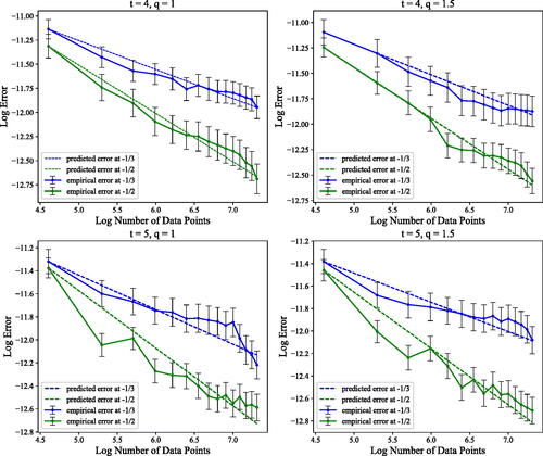
Learning Risk of Random Feature

In this experiment, we perform empirical study of the risk behavior in Theorem 1. Specifically, we first let $f_{*}(x)=k_t(x,x_0)$ for some $x_0\in (0,1)$ and $P(y|x)$ to be a Gaussian distribution with mean $f_{*}(x)$ and variance ${\sigma }^2$. We then sample the features for kernel $k_{2q}$ according to Mercer’s decomposition (Equation (14)(14) $$\begin{array}{c}K(x,y)={\lambda }_0{g}_0(x)+\sum _{i=1}{\lambda }_i\left[g_i(x)g_i(y)+h_i(x)h_i(y)\right],\\ ={\lambda }_0+2\sum _{i=1}{\lambda }_i\hspace{0.17em}\text{cos}\hspace{0.17em}\left(i2\pi (x-y)\right),\end{array}$$(14) ). Finally we perform ridge regression with regularization parameter λ and compute the excess learning risk for different values of t. According to Theorem 1, if the truncation level p and λ are proportional to $n^{-1/2}$, we should expect the risk to converge at $O(n^{-1/2})$ rate, or at $O(n^{-1/3})$ if the truncation level p and λ are proportional to $n^{-1/3}$. Figure 1 demonstrates that the empirical learning risk behavior follows this pattern for different choices of t and q.

Fig. 1 The plot of the theoretical and empirical excess risk convergence rate for various choice of the target function (represented by t) and different kernels (represented by q).

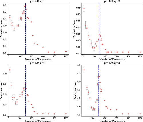
Double Descent

The final two sets of experiments aim to numerically corroborate our theoretical analysis on benign overfitting, that is, Theorem 2, Corollaries 1 and 2. To this end, we again let the target function be $f_{*}(x)=k_t(x,x_0)$ for $x_0=0.25$. We let the number of samples to be n = 300 with input distribution being uniform between 0 and 1 and label noise level of ${\sigma }^2=0.01$. For each choice of t, we construct the noisy feature matrix ${\mathbf{Z}}_{\xi }$ by appending noise into the original feature matrix Z. We then compute the prediction error of the MNLS estimator using ${\mathbf{Z}}_{\xi }$. The simulation experiment is conducted with 30 replications to compute the standard error. Finally, we plot the empirical test error against the number of features s. Figures 2 and 3 show that the empirical error displays the double descent phenomenon.

Fig. 2 The plot of the theoretical and empirical test error of MNLS estimator where target function has t = 4. Black dotted line represents the theoretical prediction and the vertical blue line is the interpolation threshold.

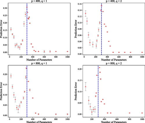
Fig. 3 The plot of the theoretical and empirical test error of MNLS estimator where target function has t = 4. Black dotted line represents the theoretical prediction and the vertical blue line is the interpolation threshold.

5 Discussion

The benign overfitting phenomenon has attracted great research interest since it was first observed by Zhang et al. (2016), Belkin, Ma, and Mandal (2018), and Belkin et al. (2019). Our article continues the lines of work of Belkin, Hsu, and Xu (2019), Bartlett et al. (2020), and Hastie et al. (2019), and focuses on developing a theoretical understanding of this phenomenon. Through analyzing the learning risk of the MNLS estimator, we first provide a nearly matching upper and lower bound for the excess learning risk and point out one possible cause of benign overfitting: the noise ξ in the covariates or in the feature vectors. Moreover, we discover that ξ plays an important implicit regularization role during learning. By incorporating ξ into our analysis, we explicitly derive how the learning risk is affected by ξ. We also provide a detailed tradeoff between the number of parameters and the learning rate, which further demonstrates the optimality in the minimax sense for the MNLS estimator. Our results may shed light on the theoretical understandings of modern deep learning, which open doors for future studies on the design of deep learning architectures. Furthermore, our results only rely on very weak assumptions of the kernel and require almost no assumption about the data generating distribution.

We believe that several extensions are worth exploring. First, although our results shed light on the two-layer neural network with fixed first layer weights, we would like to understand what would happen if we could optimize the first layer weights, that is, optimizing W in our model. Second, in the existing literature, there are many tools in analyzing neural network optimization with connection to its generalization error. Examples include the transport map formulation (Suzuki 2020), the mean-field analysis (Mei, Montanari, and Nguyen 2018; Sirignano and Spiliopoulos 2020), and the neural tangent kernel (Du et al. 2019; Jacot, Gabriel, and Hongler 2018). How to use these tools in investigating the effect of the noise ξ during neural network training would be an interesting direction. Another direction is to analyze the noise ξ in models with different loss functions.

Acknowledgments

The authors would like to thank Xufan Ma, Jean-Francois Ton, Zhongyi Hu and Chao Zhang for proofreading and fruitful discussions.

Supplementary Materials

The supplementary material contains the proof of Theorem 1 and 2 as well as Proposition 1. In additional, more experiments from Section 4 is included.

Additional information

Funding

Zhu Li is funded by the Gatsby Charitable Foundation. This research was supported in part by NSF grant CAREER DMS-1847415.

References

- Adlam, B., and Pennington, J. (2020), “The Neural Tangent Kernel in High Dimensions: Triple Descent and a Multi-Scale Theory of Generalization,” in International Conference on Machine Learning, pp. 74–84. PMLR.
- Avron, H., Kapralov, M., Musco, C., Musco, C., Velingker, A., and Zandieh, A. (2017), “Random Fourier Features for Kernel Ridge Regression: Approximation Bounds and Statistical Guarantees,” in International Conference on Machine Learning, pp. 253–262.
- Bach, F. (2017), “On the Equivalence between Kernel Quadrature Rules and Random Feature Expansions,” Journal of Machine Learning Research, 18, 1–38.
- Bartlett, P. L., Bousquet, O., Mendelson, S. (2005), “Local Rademacher Complexities,” The Annals of Statistics, 33, 1497–1537. DOI: 10.1214/009053605000000282.
- Bartlett, P. L., Long, P. M., Lugosi, G., and Tsigler, A. (2020), “Benign Overfitting in Linear Regression,” in Proceedings of the National Academy of Sciences. DOI: 10.1073/pnas.1907378117.
- Belkin, M., Hsu, D., Ma, S., and Mandal, S. (2019), “Reconciling Modern Machine-Learning Practice and the Classical Bias–Variance Trade-off,” Proceedings of the National Academy of Sciences, 116, 15849–15854.
- Belkin, M., Hsu, D., and Xu, J. (2019), “Two Models of Double Descent for Weak Features,” arXiv preprint arXiv:1903.07571.
- Belkin, M., Ma, S., and Mandal, S. (2018), “To Understand Deep Learning We Need to Understand Kernel Learning,” in International Conference on Machine Learning, pp. 541–549.
- Bochner, S. (1932), “Vorlesungen über Fouriersche Integrale,” in Akademische Verlagsgesellschaft.
- Bunea, F., Strimas-Mackey, S., and Wegkamp, M. (2020), “Interpolation under Latent Factor Regression Models,” arXiv preprint arXiv: 2002.02525.
- Caponnetto, A., and De Vito, E. (2007), “Optimal Rates for the Regularized Least-Squares Algorithm,” Foundations of Computational Mathematics, 7, 331–368. DOI: 10.1007/s10208-006-0196-8.
- Du, S., Lee, J., Li, H., Wang, L., and Zhai, X. (2019), “Gradient Descent Finds Global Minima of Deep Neural Networks,” in International Conference on Machine Learning, pp. 1675–1685. PMLR.
- Friedman, J., Hastie, T., and Tibshirani, R. (2001), The Elements of Statistical Learning, Springer Series in Statistics (Vol. 1). Berlin: Springer.
- Hastie, T., Montanari, A., Rosset, S., and Tibshirani, R. J. (2019), “Surprises in High-Dimensional Ridgeless Least Squares Interpolation,” arXiv preprint arXiv:1903.08560.
- Jacot, A., Gabriel, F., and Hongler, C. (2018), “Neural Tangent Kernel: Convergence and Generalization in Neural Networks,” in Advances in Neural Information Processing Systems, pp. 8571–8580.
- Kanagawa, M., Hennig, P., Sejdinovic, D., and Sriperumbudur, B. K. (2018), “Gaussian Processes and Kernel Methods: A Review on Connections and Equivalences,” arXiv preprint arXiv:1807.02582.
- Li, Z., Ton, J.-F., Oglic, D., and Sejdinovic, D. (2019), “Towards a Unified Analysis of Random Fourier Features,” in International Conference on Machine Learning, pp. 3905–3914.
- Li, Z., Ton, J.-F., Oglic, D., and Sejdinovic, D. (2021), “Towards a Unified Analysis of Random Fourier Features,” Journal of Machine Learning Research, 22, 1–51.
- Liang, T., and Rakhlin, A. (2020), “Just Interpolate: Kernel “Ridgeless” Regression can Generalize,” Annals of Statistics, 48, 1329–1347.
- Liang, T., Rakhlin, A., and Zhai, X. (2020), “On the Multiple Descent of Minimum-Norm Interpolants and Restricted Lower Isometry of Kernels,” in Conference on Learning Theory, pp. 2683–2711. PMLR.
- Liao, Z., Couillet, R., and Mahoney, M. W. (2020), “A Random Matrix Analysis of Random Fourier Features: Beyond the Gaussian Kernel, a Precise Phase Transition, and the Corresponding Double Descent,” arXiv preprint arXiv:2006.05013.
- Mei, S., and Montanari, A. (2019), “The Generalization Error of Random Features Regression: Precise Asymptotics and Double Descent Curve,” arXiv preprint arXiv:1908.05355.
- Mei, S., Montanari, A., and Nguyen, P.-M. (2018), “A Mean Field View of the Landscape of Two-Layer Neural Networks,” Proceedings of the National Academy of Sciences, 115, E7665–E7671.
- Rahimi, A., and Recht, B. (2007), “Random Features for Large-Scale Kernel Machines,” in Advances in Neural Information Processing Systems, pp. 1177–1184.
- Rudi, A., and Rosasco, L. (2017), “Generalization Properties of Learning with Random Features,” in Advances in Neural Information Processing Systems, pp. 3218–3228.
- Sirignano, J., and Spiliopoulos, K. (2020), “Mean Field Analysis of Neural Networks: A Central Limit Theorem,” Stochastic Processes and their Applications, 130, 1820–1852. DOI: 10.1016/j.spa.2019.06.003.
- Steinwart, I. (2019), “Convergence Types and Rates in Generic Karhunen-loève Expansions with Applications to Sample Path Properties,” Potential Analysis, 51, 361–395. DOI: 10.1007/s11118-018-9715-5.
- Steinwart, I., and Christmann, A. (2008), Support Vector Machines, New York: Springer.
- Suzuki, T. (2020), “Generalization Bound of Globally Optimal Non-convex Neural Network Training: Transportation Map Estimation by Infinite Dimensional Langevin Dynamics,” arXiv preprint arXiv:2007.05824.
- Wahba, G. (1990), Spline Models for Observational Data (Vol. 59), Philadelphia, PA: SIAM.
- Zhang, C., Bengio, S., Hardt, M., Recht, B., and Vinyals, O. (2016), “Understanding Deep Learning Requires Rethinking Generalization,” arXiv preprint arXiv:1611.03530.