Reversible Jump PDMP Samplers for Variable Selection

Abstract

A new class of Markov chain Monte Carlo (MCMC) algorithms, based on simulating piecewise deterministic Markov processes (PDMPs), has recently shown great promise: they are nonreversible, can mix better than standard MCMC algorithms, and can use subsampling ideas to speed up computation in big data scenarios. However, current PDMP samplers can only sample from posterior densities that are differentiable almost everywhere, which precludes their use for model choice. Motivated by variable selection problems, we show how to develop reversible jump PDMP samplers that can jointly explore the discrete space of models and the continuous space of parameters. Our framework is general: it takes any existing PDMP sampler, and adds two types of trans-dimensional moves that allow for the addition or removal of a variable from the model. We show how the rates of these trans-dimensional moves can be calculated so that the sampler has the correct invariant distribution. We remove a variable from a model when the associated parameter is zero, and this means that the rates of the trans-dimensional moves do not depend on the likelihood. It is, thus, easy to implement a reversible jump version of any PDMP sampler that can explore a fixed model. Supplementary materials for this article are available online.

Keywords:

• Bayesian statistics
• Bouncy particle sampler
• Model choice
• Monte Carlo
• Zig Zag Algorithm

1 Introduction

There is currently much interest in developing MCMC algorithms based on simulating piecewise deterministic Markov processes (PDMPs). These are continuous time Markov processes that have deterministic dynamics between a set of event times, and the randomness in these processes only comes through the random event times and potentially random transitions at the events (see Davis 1993, for an introduction to PDMPs).

The idea of simulating PDMPs to sample from a target distribution of interest originated in statistical physics (Peters and de With 2012; Michel, Kapfer, and Krauth 2014), but has recently been proposed as an alternative to standard MCMC to sample from posterior distributions in Bayesian Statistics, with algorithms such as the Bouncy Particle Sampler (Bouchard-Côté, Vollmer, and Doucet 2018) and the ZigZag algorithm (Bierkens and Roberts 2017; Bierkens, Fearnhead, and Roberts 2019) amongst others (Vanetti et al. 2017; Markovic and Sepehri 2018; Wu and Robert 2020; Michel, Durmus, and Sénécal 2020; Bierkens et al. 2020). See Fearnhead et al. (2018) for an introduction to this area.

To sample from a density $\pi (\mathit{\theta })$ most current PDMP samplers introduce a velocity component, v, of the same dimension as $\mathit{\theta }$, and have deterministic dynamics that correspond to a constant velocity model (though see Vanetti et al. 2017, for alternative PDMP algorithms). At the random events the velocity component changes. Algorithms differ in terms of the event rate and how the velocity changes at each event, but each has a simple recipe for choosing these so that the resulting PDMP has $\pi (\mathit{\theta })$ as its invariant distribution. These recipes depend on $\pi (\mathit{\theta })$ through the gradient of $\text{log}\hspace{0.17em}\pi (\mathit{\theta })$, which importantly means that $\pi (\mathit{\theta })$ only needs to be known up to proportionality, but also that $\pi (\mathit{\theta })$ needs to be differentiable almost everywhere. The advantages of PDMP samplers are that they are nonreversible, and thus can mix more quickly than standard reversible MCMC algorithms (Diaconis, Holmes, and Neal 2000), and, when sampling from posterior distributions, they can use a small sample of data points at each iteration whilst still targeting the true posterior distribution (Bierkens, Fearnhead, and Roberts 2019).

However, the restriction to sampling from densities that are differentiable means that current PDMP samplers cannot be used in model choice problems. The aim of this article is to address this limitation, with a particular motivation of PDMP samplers that can be used in variable selection problems that are common in, for example, linear regression and generalized linear models. We show how to design efficient PDMP samplers which allow movement between different models.

A simple way to implement PDMP samplers for variable selection problems is to use continuous spike-and-slab priors on the parameters (George and McCulloch 1993; Ishwaran and Rao 2005), which, rather than setting some parameters exactly to 0, have priors that place substantial mass close to 0. With such a prior, the resulting posterior density is differentiable, and existing PDMP samplers can be used (Goldman, Sell, and Singh 2021). However, such an approach has three disadvantages. First, under such a prior it can be hard to interpret the results as we do not formally get posterior probabilities on whether certain variables should be included in the model. Second, they introduce an extra tuning parameter to the prior which governs the shape of the spike of the component. Third, as we show in Section 2.2, using PDMP samplers to sample from the resulting posterior can be computationally inefficient: the samplers will need to simulate many events so that the parameters associated to variables that should not be in the model are kept close to 0.

We demonstrate how to adapt existing PDMP samplers to variable selection problems. Specifically they evolve as the PDMP sampler when exploring the posterior associated with a given model, but with two additional events: if any parameter value hits 0 the PDMP jumps to the smaller model where the corresponding variable is removed; whilst with some rate there are events that reintroduce variables into the model. We show in Section 3 how to calculate the rate and transition for these new types of event so that the sampler has the correct invariant distribution. To calculate these we need different techniques than those used for existing PDMP samplers, as we need to account for the behavior of the process when parameters hit zero. The techniques we use are most similar to those in Bierkens et al. (2018), which considers PDMPs with restricted domains. However, in that paper the dynamics at the boundary of the domain could be chosen so that the net flow of probability at the boundary is zero; whereas we need to balance the probability flow out of a model which occurs when a parameter hits zero with the flow into the model caused by the events that reintroduce variables.

Our approach is not the only way of extending PDMP samplers to the variable selection problem. One could also introduce moves that propose adding or deleting a variable from the model regardless of the current state of the PDMP. Such ideas have been proposed for other continuous-time samplers, see Grenander and Miller (1994) or Phillips and Smith (1996) for their use within jump-diffusion samplers, and Stephens (2000) for their use within continuous-time Markov jump process samplers. Exactly the same type of moves between models could be implemented for PDMPs. However, we believe our approach, that only allows removing variables when the corresponding parameter value hits zero, has important practical advantages. Most importantly, because we add or remove a variable when its corresponding parameter is 0 the rates of these events do not depend on the likelihood, but only the prior. This makes simulating these events simple—in fact for many common priors the rate at which we add a variable will be constant. Thus, any PDMP sampler suitable for a fixed model can easily be extended to allow for variable selection. By comparison the moves and rates described in Grenander and Miller (1994) would involve rates that depend on the likelihood ratio between the current and new model. Simulating events with this rate will be challenging, as the rate will vary, in a complicated way, when the parameter values change. Calculating this rate will be costly as it requires evaluating the log-likelihood, which is a sum over the data points. Furthermore, most algorithms to simulate events require bounds on the rates, and calculating good bounds will be problem specific and potentially difficult. After a preprint of this work appeared (Chevallier, Fearnhead, and Sutton 2020), a related method, called the sticky PDMP (Bierkens et al. 2021), has been proposed. For variable selection problems, the main difference between the two approaches is that the sticky PDMP sampler remembers the velocity of a component when it is re-added back into the model, and thus will continue in the same direction as it was moving before that variable was removed.

The approach we present is generic, in that it can take any current PDMP sampler and be used to obtain a version that can be applied to the variable selection problem. We call the new class of samplers reversible jump PDMP samplers, due to the analogy with reversible jump MCMC (Green 1995), though the class of moves we allow are less general than those available for standard reversible jump MCMC. We show how to derive reversible-jump versions of both ZigZag and the Bouncy Particle Sampler in Section 4, before investigating empirically these algorithms on both logistic regression and robust linear regression models.

Proofs of all theorems are relegated to the supplementary materials. Code for implementing the new reversible jump PDMP samplers is available from the R package rjpdmp available from the Comprehensive R Archive Network (CRAN).

2 PDMP Samplers and Model Choice

2.1 Variable Selection

We will consider model selection problems that arise from variable selection. The general framework is that we have a vector of parameters, $\mathit{\theta }=({\theta }_1,\dots ,{\theta }_d)$, and each model is characterized by setting some subset of the θ_js to 0. This is a common setting across linear models, generalized linear models and various extensions.

To make ideas concrete, consider a linear model $$\mathit{Y}=\sum _{j=1}^d{\mathit{X}}_j{\theta }_j+ϵ$$where Y is a vector of response variables, each ${\mathit{X}}_j$ is a vector of covariates, and ϵ is an additive noise vector. When d is large it is common to fit such a model under a sparsity assumption, namely that many of the θ_js are 0.

In a Bayesian analysis, such a sparsity assumption is encapsulated in our choice of prior on $\mathit{\theta }$. To aid interpretation of the variable selection priors it is common to introduce a latent variable $\mathit{\gamma }=({\gamma }_1,\dots ,{\gamma }_d)\prime$ where ${\gamma }_j=1$ if the covariate ${\mathit{X}}_j$ is included in the model, that is, if ${\theta }_j\ne 0$. We let $\left|\mathit{\gamma }\right|=\sum {\gamma }_j$ be the number of covariates included in the corresponding model. Indexing ${\mathit{\theta }}_{\mathit{\gamma }}$ as the sub-vector of $\mathit{\theta }$ with only the selected variables, any prior can be written in a hierarchical form where we have a prior on $\mathit{\gamma }$, then conditional on $\mathit{\gamma }$ we have a prior on ${\mathit{\theta }}_{\mathit{\gamma }}$, and set all remaining entries of $\mathit{\theta }$ to 0.

A special case is where each component of $\mathit{\theta }$ is independent of the others. In which case the prior can be written as $${\theta }_j\sim w_j{g}_j({\theta }_j)+(1-w_j){\delta }_0({\theta }_j),\hspace{1em}\hspace{1em}j=1,\dots ,d,$$where $w_j\in (0,1)$ is the prior probability that ${\gamma }_j=1$, δ₀ is a Dirac measure at zero and $g_j({\theta }_j)$ is a distribution that models our prior beliefs for θ_j conditional on that variable being included in the model. Bayesian approaches to variable selection that put a probability mass on ${\theta }_j=0$ in this way will be referred to as Dirac spike and slab methods. Notable examples of these methods include Mitchell and Beauchamp (1988), Kuo and Mallick (1998), Geweke (1996), Smith and Kohn (1996), and Bottolo and Richardson (2010).

While this formulation is natural from a modeling perspective, sampling from the resulting posterior distribution can be challenging, with, for example, MCMC samplers that use gradient information such as Hamiltonian Monte Carlo (Neal 2011) not being applicable. To circumvent this issue it is common to use an approximation to this prior which replaces the point mass at 0 with a density that is peaked around 0, such as (1) $${\theta }_j\sim w_j\mathcal{N}(0,{\tau }_j^2)+(1-w_j)\mathcal{N}(0,{\tau }_j^2{c}_j^2),\hspace{1em}\hspace{1em}j=1,\dots ,d,$$(1) where c_j is taken small so that $\mathcal{N}(0,c_j^2{\tau }_j^2)$ approximates the Dirac spike. We will refer to Bayesian variable selection methods that replace the Dirac in the prior with a continuous approximation as continuous spike-and-slab methods.

2.2 PDMP Samplers

Piecewise Deterministic Markov Processes (PDMPs) are an emerging class of nonreversible continuous-time samplers. We will consider sampling from a distribution with density $\pi (\mathit{\theta })$ defined on some space $\mathcal{X}$. Current samplers augment the state to include a velocity vector and sample from a distribution on $E=\mathcal{X}\times \mathcal{V}$. In the following, for $\mathit{z}\in E$ we will use the notation $\mathit{z}=(\mathit{\theta },\mathit{v})$ with $\mathit{\theta }\in \mathcal{X}$ a position and $\mathit{v}\in \mathcal{V}$ a velocity.

A PDMP can be defined by (i) deterministic dynamics between a set of random event times; (ii) the state-dependent rate at which events occur, $\lambda (\mathit{z})$; and (iii) a probability distribution for the change in state at each event, with density $q(\mathit{z}\prime |\mathit{z})$. We will consider PDMPs whose deterministic trajectories follow a differential equation of the form: $$\frac{\mathrm{d}({\mathit{\theta }}_t,{\mathit{v}}_t)}{\mathrm{d}t}=({\mathit{v}}_t,\Phi ({\mathit{\theta }}_t,{\mathit{v}}_t))$$with $\Phi :E\to \mathcal{V}$ a smooth function. This setting contains the usual PDMP samplers such as ZigZag (Bierkens, Fearnhead, and Roberts 2019), the Bouncy Particle Sampler (Bouchard-Côté, Vollmer, and Doucet 2018), or the Coordinate Sampler (Wu and Robert 2020).

For example, the ZigZag algorithm to simulate from $\pi (\mathit{\theta })$ for $\mathit{\theta }\in {\mathbb{R}}^d$, would introduce a velocity vector $\mathit{v}\in {\{-1,1\}}^d$, and deterministic dynamics $$\frac{\mathrm{d}({\mathit{\theta }}_t,{\mathit{v}}_t)}{\mathrm{d}t}=({\mathit{v}}_t,0),$$which are the dynamics of a constant velocity model. For ZigZag, events occur at a rate that depends on the gradient of $\pi (\mathit{\theta })$ in each component of the velocity, and at an event one component of the velocity is switched. The rate at which the jth component of the velocity, ${\mathit{v}}_t^j$, is switched is just $$\max \left\{0,-{\mathit{v}}_t^j\frac{\partial }{\partial {\mathit{\theta }}^j}\text{log}\hspace{0.17em}\pi ({\mathit{\theta }}_t)\right\}.$$

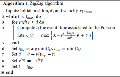
These rates depend on the target distribution just through the gradient of the log of the target—which importantly means that we need only know the target distribution up to proportionality. Algorithm 1 gives computational pseudocode for simulating from the ZigZag process.

We can apply current PDMPs, such as ZigZag, to the Bayesian variable selection problem if we use the continuous spike-and-slab prior (1). Realizations of such a sampler are shown in the left two plots of Figure 1 as we vary how concentrated the spike distribution is. For the more concentrated case, the sampler becomes inefficient as it involves many switching events when the state variable is close to 0.

Fig. 1 Sample paths of PDMPs implementing variable selection in one dimension. The left and centre plots show the trajectories for a continuous spike-and-slab prior $0.5\mathcal{N}(0,{\tau }^2)+0.5\mathcal{N}(0,{\tau }^2{c}^2)$ where ${\tau }^2=16$. As c decreases the spike component in the mixture approaches a Dirac mass. The figure on the right is the limiting process where we set the velocity to zero allowing the variable to stay fixed at zero.

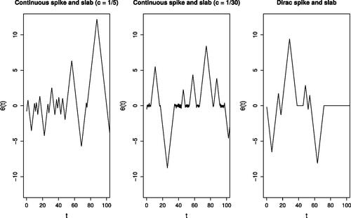
Intuitively as we make the variance of the spike component of the prior tend to 0 the prior converges to a prior with a point mass at 0; furthermore we can observe the output of our PDMP sampler “converging” to a process shown in the right-hand plot of Figure 1. Here, rather than the state having periods where it oscillates around 0, it has periods of time where ${\theta }_j=0$ and thus has many fewer events. This limiting process motivates the new class of PDMP samplers that we develop.

3 Reversible Jump PDMP Samplers

Let $\mathcal{M}=({\mathcal{M}}_1,{\mathcal{M}}_2,\dots )$ be a set of models indexed by a parameter k. Each model, ${\mathcal{M}}_k$, has a corresponding state space ${\mathcal{X}}^k$ of dimension d_k. For the sake of clarity, we will limit ourselves to variable selection. In our case ${\mathcal{X}}^k$ has a specific form: $${\mathcal{X}}^k=\prod _i{\mathbb{R}}^{{\gamma }_i^k}$$where we abuse notation by using ${\mathbb{R}}^0=\left\{0\right\}$ and where $({\gamma }_i^k)$ is a sequence of numbers in {0, 1} representing whether a variable is enabled for model ${\mathcal{M}}_k$. Let π be the target posterior defined on $\mathcal{X}={\cup }_k{\mathcal{X}}^k$. We further assume that the restriction of π to each ${\mathcal{X}}^k$ has a density, and denote this by ${\pi }_k(\mathit{\theta })$. The first ingredient of our sampler is a collection of PDMPs defined for each model. Each PDMP sampler adds a velocity space ${\mathcal{V}}^k$ to the space ${\mathcal{X}}^k$ and samples from the space $E_k={\mathcal{X}}^k\times {\mathcal{V}}^k$. Finally, for each model ${\mathcal{M}}_k$, the associated PDMP sampler has an invariant distribution proportional to ν_k, where $${\nu }_k(\mathit{\theta },\mathit{v})={\pi }_k(\mathit{\theta })p_k(\mathit{v}|\mathit{\theta })\hspace{1em}\hspace{1em}(\mathit{\theta },\mathit{v})\in {\mathcal{X}}^k\times {\mathcal{V}}^k,$$ for some set of conditional densities $p_k(\mathit{v}|\mathit{\theta })$.

Remark 1

. For samplers such as ZigZag, $p_k(\mathrm{d}\mathit{v}|\mathit{\theta })$ is a measure with support on a discrete set—it places probability mass $1/2^k$ on each of the possible $2^k$ velocities allowed by ZigZag. By choosing ${\mathcal{V}}^k$ to be the support of $p_k(\mathrm{d}\mathit{v}|\mathit{\theta }),\hspace{0.17em}{p}_k(\mathrm{d}\mathit{v}|\mathit{\theta })$ still has a density—and integrals can be interpreted as sums over the support points. This allows us to treat all samplers within the same framework.

The second ingredient of our reversible jump PDMP sampler is a set of jumps between models. For our case of variable selection, we only allow adding or removing one variable at a time. Hence, let $$\begin{array}{c}\mathcal{T}=\{(i,j) | \text{there exists a }k \text{such that} {\gamma }_k^i=1,{\gamma }_k^j=0;\\ \hspace{1em} \text{and} {\gamma }_l^i={\gamma }_l^j,l\ne k\}\end{array}$$be a set of pairs of transitions between models, with these ordered (i, j) such that model ${\mathcal{M}}_j$ is obtained from ${\mathcal{M}}_i$ by removing one of the variables in ${\mathcal{M}}_i$. For transition $i\to j$, we define an active boundary ${\Gamma }_{i,j}={\mathcal{X}}^j\times {\mathcal{V}}^i\subset E_i$, a subspace of E_i. Each trajectory passing through ${\Gamma }_{i,j}$ has some probability $p_{i,j}$ of jumping to E_j using a deterministic jump function $g_{i,j}:{\Gamma }_{i,j}\to E_j$. We assume that the jump function does not change the parameter $\mathit{\theta }$. So, if a trajectory ${\mathit{z}}_t$ of our process has a left limit at time t, ${\mathit{z}}_{t-}$ in ${\Gamma }_{i,j}$, then with some probability $p_{i,j},\hspace{0.17em}{\mathit{z}}_t=g_{i,j}({\mathit{z}}_{t-})\in E_j$ with ${\mathit{\theta }}_t={\mathit{\theta }}_{t-}$. For transition $j\to i$, we introduce a Poisson rate, ${\beta }_{i,j}(\mathit{z})$, and a jump kernel, $Q_{i,j}(·|\mathit{z})$, such that if the trajectory is in E_j, then with rate ${\beta }_{i,j}({\mathit{z}}_{t-}),\hspace{0.17em}{\mathit{z}}_t$ is drawn from $Q_{i,j}(·|{\mathit{z}}_{t-})\in {\Gamma }_{i,j}$. We impose symmetry in the jumps between models so that for any $\mathit{z}\prime \sim Q_{i,j}(·|\mathit{z}),\hspace{0.17em}{g}_{i,j}(\mathit{z}\prime )=\mathit{z}$, that is, the probability measure $Q_{i,j}(·|\mathit{z})$ is supported by $g_{i,j}^{-1}(\mathit{z})$.

As an example, for the ZigZag sampler, where velocities are plus or minus 1 in each component, we could choose the function $g_{i,j}(\mathit{z})$ that sets the velocity associated with the variable that is removed from the model to 0 and keeps other components unchanged. The reverse transition, defined by $Q_{i,j}$, would then need to sample the velocity component associated with the added velocity component from $\{-1,1\}$, and leave other components unchanged. If we have a sampler where the velocity is constrained to lie in the sphere, that is $\mathit{v}·\mathit{v}=1$ we cannot just set a component v to 0, as the resulting velocity will no longer lie on the sphere. Instead, $g_{i,j}$ could set the appropriate component of v to 0 and then renormalize the velocity. The reverse transition could propose a value of the velocity for the added component, from $[-1,1]$, and then rescale the other velocity components.

3.1 Invariant Distribution

Let $\nu =\sum _k{\nu }_k$ be a measure on ${\cup }_k{E}_k$, where ν_k is the invariant distribution of the base PDMP restricted to E_k. By construction, the $\mathit{\theta }$-marginal distribution of ν is π and this section provides sufficient conditions on $Q_{i,j},p_{i,j}$, and ${\beta }_{i,j}$ for ν to be an invariant distribution of the process.

To get a directly usable conditions on ${\beta }_{i,j},p_{i,j},$ and $Q_{i,j}$ that ensure the target measure is invariant, some additional notation must be introduced. When jumping from $\mathit{z}=(\mathit{\theta },\mathit{v})\in E_j$ to $\mathit{z}\prime =(\mathit{\theta },\mathit{v}\prime )\in E_i$, the dimension of the velocity vector needs to be increased by one, but the position is unchanged. (Strictly speaking, the position also increases in dimension by one, but the additional position variable is set to 0.) Hence, $g_{i,j}^{-1}(\mathit{z})$ is a one-dimensional manifold, which can be related to a subset, U say, of $\mathbb{R}$ by introducing a function $$G_{i,j}:U\times E_j\to E_i$$such that for any $\alpha \in U$, we have $G_{i,j}(\alpha ,\mathit{z})\in g_{i,j}^{-1}(\{\mathit{z}\})$ and for a fixed $\mathit{z}\in E_j,\hspace{0.17em}\alpha \mapsto G_{i,j}(\alpha ,\mathit{z})$ is a one-to-one mapping from U to $g_{i,j}^{-1}(\mathit{z})$ (similar ideas are seen in reversible jump MCMC; see Green 1995). For a given $\mathit{z}\in E_j$, it is natural to rewrite the jump kernel $Q_{i,j}$ in terms of $\alpha \in U$, and henceforth we abuse notation and write $Q_{i,j}(·|\mathit{z})$ as a density on U. That is we can simulate the transition from E_j to E_i, by simulating $\alpha \sim Q_{i,j}(·|\mathit{z})$ and then setting $\mathit{z}\prime =G_{i,j}(\alpha ,\mathit{z})$.

So for the ZigZag sampler, where $g_{i,j}$ sets a component of the velocity to 0, $g_{i,j}^{-1}(\mathit{z})$, will be equal to the set of two states that have the same position as z and whose velocities are identical to that of z except for the component associated with the added variable. The two velocities in this set would correspond to replacing the velocity of 0 for that component with either 1 or –1. In this case U would just be the value of the velocity associated with the added component. We can simulate from the reverse transition by simulating U and calculating the new velocity from the old state z and U—this mapping defines $G_{i,j}$.

Finally, define ${\mathit{n}}_{i,j}$ to be a normal to the boundary ${\Gamma }_{i,j}$ and let (2) $${\nu }_{i,j}(\mathit{z})=\nu (\mathit{z})|〈\mathit{v},{\mathit{n}}_{i,j}〉|$$(2) be an unnormalized density on ${\Gamma }_{i,j}$ and let ${\overline{\nu }}_{i,j}$ be the pushforward measure on E_j of ${\nu }_{i,j}$ by $g_{i,j}$: (3) $${\overline{\nu }}_{i,j}(B)={\int }_{g_{i,j}^{-1}(B)}{\nu }_{i,j}(\mathit{z})\mathrm{d}\mathit{z} \text{for} \text{any} B\subset E_j\hspace{0.17em}\text{measurable}.$$(3)

Informally this is the measure under ${\nu }_{i,j}$ associated with values of $\mathit{\theta }\in {\Gamma }_{i,j}$ that would be mapped by $g_{i,j}$ to the set B.

For our example of the ZigZag sampler, $|〈\mathit{v},{\mathit{n}}_{i,j}〉|=1$ as velocities are defined so that they are ±1 in all directions normal to the boundaries. Thus, ${\nu }_{i,j}(\mathit{z})$ is just the un-normalized density of z under $\nu (\mathit{z})$ restricted to $\mathit{z}\in {\Gamma }_{i,j}$. The push-forward measure ${\tilde{\nu }}_{i,j}$ for a set B in the space of the smaller model is just the measure under ${\nu }_{i,j}$ of all the values of the state z on the boundary ${\Gamma }_{i,j}$ of the larger model that would be mapped to B when we moved model. That is, for a state in B we consider the pair of states that have the same position and whose velocity is the same except that the velocity of 0 at the removed component is replaced with 1 or –1, and calculate the measure of all such pairs of states corresponding to states in B.

We now present our conditions on ${\beta }_{i,j},\hspace{0.17em}{Q}_{i,j}$ and $p_{i,j}$. It is helpful to consider separately the cases where the space of velocities is continuous and the case where it is discrete.

Theorem 1

. Assume the space of velocities is continuous, that for each k, the base PDMP on E_k has ν_k as its invariant distribution, and define $\lambda (\mathit{z})$ for $\mathit{z}\in E_k$ to be the jump rate of the base PDMP on E_k. Further assume:

1. the mean jump rate of the base PDMPs is finite, that is, $\int \lambda (\mathit{z})\mathrm{d}\nu <\infty$;

2. for all k, π_k is in C¹, that is, continuously differentiable, on ${\mathcal{X}}_k$;

3. for any k, and any $\mathit{v}\in {\mathcal{V}}^k,\hspace{0.17em}{\int }_{{\mathcal{X}}_k}|\nabla {\pi }_k(\mathit{\theta })·\mathit{v}|\mathrm{d}\mathit{\theta }<\infty$.

Then the measure ν is invariant if for every $(i,j)\in \mathcal{T}$, the following conditions hold (4) $${\beta }_{i,j}(\mathit{z})=p_{i,j}\frac{{\overline{\nu }}_{i,j}(\mathit{z})}{\nu (\mathit{z})} \text{for} \mathit{z}\in E_j$$(4) (5) $$Q_{i,j}(\alpha |\mathit{z})=\frac{{\nu }_{i,j}(G_{i,j}(\alpha ,\mathit{z}))|J_{G_{i,j}}(\alpha ,\mathit{z})|}{{\overline{\nu }}_{i,j}(\mathit{z})}\hspace{1em}\hspace{1em}\text{for} \mathit{z}\in E_j \text{and} \alpha \in U,$$(5) where $J_{G_{i,j}}$ denotes the Jacobian associated with the transformation $G_{i,j}$.

Proof.

See supplementary materials. □

Intuitively, this result can be understood as a detailed balance condition: we balance the probability flow for each jump $\mathit{z}\to \mathit{z}\prime$ from E_i to E_j, with that of the reverse jump $\mathit{z}\prime \to \mathit{z}$.

For discrete velocity spaces the result is slightly simpler, as the Jacobian term is not required. In this case we replace (5) with the condition (6) $$Q_{i,j}(\alpha |\mathit{z})=\frac{{\nu }_{i,j}(G_{i,j}(\alpha ,\mathit{z}))}{{\overline{\nu }}_{i,j}(\mathit{z})}\hspace{1em}\hspace{1em} \text{for} \mathit{z}\in E_j \text{and} \alpha \in U.$$(6)

3.2 A Reversible Jump PDMP Algorithm

Pseudo-code outlining how we can simulate the resulting Reversible Jump PDMP is given in Algorithm 2. In Lines 2–12, we loop over possible events—which can either be events where we jump to a model with an additional active variable, a component of the PDMP position hitting zero, or events within the base PDMP—and simulate the times for each of these possible events. In Lines 13–17 we calculate when the first of these possible events occurs and update the process to that time. In Lines 18–32 we then update the PDMP state based on which type of event has occurred.

In this algorithm, the additional computational cost of the reversible jump moves, over and above the cost of simulating the base PDMP sampler, is proportional to the number of variables. For each active variable we have to calculate the next time its position hits 0, which involves solving a scalar linear equation. For each inactive variable we need to simulate the time at which we next introduce the variable. As we show in the next section, in most cases the rates for these event are simple, often constant, and importantly do not depend on the likelihood. In practice more efficient implementations than Algorithm 2 will be possible that reuse previously simulated times of events. For example, if an event does not change the velocity associated with a given variable, then we do not need to recalculate the time that variable hits 0.

4 Example Samplers

4.1 ZigZag Sampler

We first derive the jump rates and transitions for the ZigZag sampler described in Section 2.2.

We choose $g_{i,j}$ to be the orthogonal projection, that is the projection that sets the velocity of the disabled variable to 0. Let $(i,j)\in \mathcal{T}$ be a transition. For any $\mathit{v}\in {\mathcal{V}}^i$, we have $|〈\mathit{v},{\mathit{n}}_{i,j}〉|=1$, thus from our definition of ${\nu }_{i,j}(\mathit{z})$ in (2) $${\nu }_{i,j}(\mathit{z})=\nu (\mathit{z})={\pi }_i(\mathit{\theta })2^{-\left|{\gamma }_i\right|}.$$

For $\mathit{z}\in E_j$, since a velocity component in $\{-1,1\}$ is projected to 0, then from (3) $${\overline{\nu }}_{i,j}(\mathit{z})=2{\pi }_i(\mathit{\theta })2^{-\left|{\gamma }_i\right|}={\pi }_i(\mathit{\theta })2^{-\left|{\gamma }_j\right|}.$$

Since $g_{i,j}$ is the projection that sets to 0 the disabled variable, $g_{i,j}^{-1}(\mathit{\theta },\mathit{v})=\{(\mathit{\theta },\mathit{v}+{\mathit{n}}_{i,j}),(\mathit{\theta },\mathit{v}-{\mathit{n}}_{i,j})\}$ and denoting the new velocity of the added component by $\alpha \in \{-1,1\}$, we chose $$G_{i,j}(\alpha ,\mathit{\theta },\mathit{v})=\alpha {\mathit{n}}_{i,j}+\mathit{v}.$$

Furthermore, we have from the version of Theorem 1 for discrete velocity spaces that (7) $${\beta }_{i,j}(\mathit{z})=p_{i,j}\frac{{\pi }_i(\mathit{\theta })}{{\pi }_j(\mathit{\theta })}$$(7) (8) $$Q_{i,j}(\alpha |\mathit{z})=1/2\hspace{1em}\text{for} \alpha \in \{-1,1\}.$$(8)

For our variable selection problem, the ratio of the posterior density that appears in ${\beta }_{i,j}$ will simplify to the ratio of the priors as the likelihood terms are common and cancel. If we have independent priors on the parameters for each variable this term will be a constant, which simplifies the simulation of the events at which we add new variables into our model. This comment applies also to the rates for the Bouncy Particle Sampler which we derive next. See the Supplementary Material for pseudocode for simulating from this process.

4.2 Bouncy Particle Sampler

We consider two versions of the Bouncy Particle Sampler. The first version has velocities on the unit sphere, so $${\mathcal{V}}^i=\{\mathit{v}\in {\mathbb{R}}^{\left|{\gamma }^k\right|} \text{such} \text{that} |\left|\mathit{v}\right||=1\}.$$

Like the ZigZag sampler, the deterministic dynamics are given by a constant velocity model. The event rate for sampling from a density ${\pi }_k(\mathit{\theta })$ is $$\lambda (\mathit{z})=\max \{0,-\mathit{v}·{\nabla }_{\mathit{\theta }}\hspace{0.17em}\text{log}\hspace{0.17em}{\pi }_k(\mathit{\theta })\},$$with the velocity reflecting in the normal to $\text{log}\hspace{0.17em}{\pi }_k(\mathit{\theta })$ at an event: if ${\mathit{n}}_k(x)$ is the normal to $\text{log}\hspace{0.17em}{\pi }_k(\mathit{\theta })$, then the new velocity is $$\mathit{v}\prime =\mathit{v}-2\left(\frac{\mathit{v}·{\mathit{n}}_k(x)}{{\mathit{n}}_k(x)·{\mathit{n}}_k(x)}\right){\mathit{n}}_k(x).$$

The Bouncy Particle Sampler also often has refresh events, at which a completely new velocity is sampled.

Extending the Bouncy Particle Sampler to the variable selection problem requires a more careful analysis than for the ZigZag sampler due to the geometry of the velocity space. Since velocities lie in the unit sphere, we choose $g_{i,j}$ to be the orthogonal projection followed by a rescaling. Hence, $g_{i,j}^{-1}(\mathit{\theta },\mathit{v})=\left\{\right(\mathit{\theta },\alpha {\mathit{n}}_{i,j}+\sqrt{1-{\alpha }^2}\mathit{v}\left)\right|\alpha \in [-1,1]\}$ and denoting the new velocity of the added component by $\alpha \in [-1,1]$, we chose $$G_{i,j}(\alpha ,\mathit{\theta },\mathit{v})=\alpha {\mathit{n}}_{i,j}+\sqrt{1-{\alpha }^2}\mathit{v}.$$

The following proposition states how to choose the jump rate, ${\beta }_{i,j}$ and the density for α.

Proposition 1

. For the Bouncy Particle Sampler with velocities on the unit sphere, (4) and (5) are satisfied if, for all $(i,j)\in \mathcal{T}$ with $\left|{\gamma }^j\right|>0$: $$\begin{array}{c}{\beta }_{i,j}(\mathit{z})=p_{i,j}\frac{{\pi }_i(\mathit{\theta })}{{\pi }_j(\mathit{\theta })}\frac{2A_{\text{sphere}}(|{\gamma }^j|)}{A_{\text{sphere}}(|{\gamma }^i|)}\frac{1}{\left|{\gamma }^j\right|}\\ Q_{i,j}(\alpha |\mathit{z})=\frac{\left|\alpha \right|\left|{\gamma }^j\right|{\sqrt{1-{\alpha }^2}}^{\left|{\gamma }^j\right|-2}}{2} \text{for} \mathit{z}\in E_j \text{and} \alpha \in (-1,1)\end{array}$$with $A_{\text{sphere}}(|{\gamma }^i|)=\frac{\Gamma \left(\frac{\left|{\gamma }^i\right|}{2}\right)}{2{\pi }^{\frac{\left|{\gamma }^i\right|}{2}}}$ the area of the unit sphere of ${\mathbb{R}}^{\left|{\gamma }^i\right|}$; and if $\left|{\gamma }^j\right|=0$, where the Bouncy Particle Sampler and ZigZag are equivalent, we use (7) and (8).

The second version of the Bouncy Particle Sampler has velocities in ${\mathbb{R}}^{\left|{\gamma }^k\right|}$, with their density being standard Gaussian and independent of $\mathit{\theta }$. The dynamics are as previously. The geometry of this case is simpler and we choose $g_{i,j}$ to be the orthogonal projection of the velocity. Hence, $g_{i,j}^{-1}(\mathit{\theta },\mathit{v})=\{(\mathit{\theta },\mathit{v}+\alpha {\mathit{n}}_{i,j})|\alpha \in \mathbb{R}\}$ and we chose $$G_{i,j}(\alpha ,\mathit{\theta },\mathit{v})=\alpha {\mathit{n}}_{i,j}+\mathit{v}.$$

Proposition 2

. For the Bouncy Particle Sampler with Gaussian velocities, (4) and (5) are satisfied if, for all $(i,j)\in \mathcal{T}$: $$\begin{array}{c}{\beta }_{i,j}(\mathit{z})=p_{i,j}\frac{{\pi }_i(\mathit{\theta })}{{\pi }_j(\mathit{\theta })}\frac{2}{\sqrt{2\pi }}\\ Q_{i,j}(\alpha |\mathit{z})=2|\alpha |e^{-\frac{1}{2}{\alpha }^2} \text{for} \mathit{z}\in E_j \text{and} \alpha \in \mathbb{R}.\end{array}$$

5 Simulation Study

In this section we demonstrate the potential advantage of our new samplers compared to alternative approaches for Bayesian variable selection. To compare between different samplers we consider the Monte Carlo estimates of the posterior probabilities of inclusion, the posterior means for the regression coefficients, and the posterior means conditioned on the model. For a given sampler the statistical efficiency is measured by the mean squared error of the sampler, denoted by ${\sigma }_{\text{sampler}}^2$, and is calculated using R runs of the sampler as (9) $${\sigma }_{\text{sampler}}^2=\frac{1}{R}\sum _{i=1}^R{({\widehat{q}}_r-q)}^2$$(9) where ${\widehat{q}}_r$ for $r=1,\dots ,R$ are the estimates of a quantity of interest from the R runs, and q is either the exact posterior quantity of interest, if available, or it is the estimate from an independent long run of an MCMC method. In multiple dimensions the statistical efficiency is measured as the median ${\sigma }_{\text{sampler}}^2$ over all dimensions. To compare the performance of different samplers we also consider a measure of efficiency relative to a reference sampler. If we denote the reference sampler by ref, then we define Relative Statistical Efficiency (RSE) and Relative Efficiency (RE) by $$\text{RSE}=\frac{{\sigma }_{\text{ref}}^2 n_{\text{ref}}}{{\sigma }_{\text{sampler}}^2 n_{\text{sampler}}},\hspace{1em}\hspace{1em}\text{RE}=\frac{{\sigma }_{\text{ref}}^2 t_{\text{ref}}}{{\sigma }_{\text{sampler}}^2 t_{\text{sampler}}},$$ where $n_{\text{sampler}}$ and $n_{\text{ref}}$ are the number of iterations of the algorithms and $t_{\text{sampler}}$ and $t_{\text{ref}}$ are the computation times of the algorithms. The RSE measures the relative efficiency of the algorithms per iteration whereas the RE measures the efficiency per second. For interpretation, an RSE or RE value of 2 implies that the sampler is 2 times more efficient than the reference method. The sensitivity of the methods to the choice of reversible jump parameters $p_{i,j}$ and regular PDMP tuning parameters is explored empirically in the Supplementary Material. Based on these results we fixed $p_{i,j}=0.6$ for all i and j in all reversible jump PDMP samplers and implemented BPS with normal velocity distribution with a fixed refreshment rate of 0.1 that was constant across models. We set this rate to be 0.1 based on results from some initial tuning runs.

5.1 Logistic Regression

First we compare PDMP based samplers with existing MCMC methods for a logistic regression model with spike and slab priors on the regression coefficients. The MCMC competitors are a collapsed Gibbs sampler, and two reversible jump samplers. The Gibbs sampler uses the Polya-Gamma augmentation of Polson, Scott, and Windle (2013) to make efficient moves through model space. We implemented one reversible jump MCMC sampler using the NIMBLE software package (de Valpine et al. 2017) using an independent normal proposal for selected variables. The other is a reversible-jump version of HMC, which, at each iteration, with probability 1/2 uses an HMC move within a model, and otherwise uses a reversible jump move between models. More details on the samplers are given in the Supplementary Material.

The logistic regression model has a d-dimensional regression parameter $\mathit{\theta }\in {\mathbb{R}}^d$, and a binary response $y_i\in \{0,1\}$ which is distributed as $$P(y_i=1|{\mathit{x}}_i,\mathit{\theta })=\frac{\hspace{0.17em}\text{exp}\hspace{0.17em}(\sum _{j=1}^d{x}_{i,j}{\theta }_j)}{1+\hspace{0.17em}\text{exp}\hspace{0.17em}(\sum _{j=1}^d{x}_{i,j}{\theta }_j)}$$where ${\mathit{x}}_i$ is the d-vector of covariates for observation i. In our simulation study, each vector ${\mathit{x}}_i$ is simulated from a multivariate normal with mean zero and d × d covariance matrix $\mathbf{\Sigma }$. We use a prior that is independent for each θ_j and where ${\theta }_j\sim \frac{10}{d}\mathcal{N}(0,10)+(1-\frac{10}{d}){\delta }_0$, which corresponds to a prior that favors models with 10 selected variables. Data was generated using this model and the following choices for $\mathit{\theta }$ and covariance matrix $\mathbf{\Sigma }$:

1. A pair of correlated covariates, one of which is in the model: $\mathit{\theta }={(1,0,\dots 0)}^T$ with ${\mathbf{\Sigma }}_{2,1}={\mathbf{\Sigma }}_{2,1}=0.9,\hspace{0.17em}{\mathbf{\Sigma }}_{i,i}=1$, and ${\mathbf{\Sigma }}_{i,j}=0$ otherwise.

2. Structured correlation between all covariates with six active covariates:

   $\mathit{\theta }={(3,3,-2,3,3,-2,0,\dots ,0)}^T$ with ${\mathbf{\Sigma }}_{i,j}=\hspace{0.17em}\text{exp}\hspace{0.17em}(-|i-j|)$.

3. No correlation between covariates and six active covariates:

   $\mathit{\theta }={(3,3,-2,3,3,-2,0,\dots ,0)}^T$, with ${\mathbf{\Sigma }}_{i,i}=1$ and ${\mathbf{\Sigma }}_{i,j}=0$ if $i\ne j$.

4. Multiple pairs of correlated variables with six active covariates:

   $\mathit{\theta }={(3,3,-2,3,3,-2,0,\dots ,0)}^T$ with ${\mathbf{\Sigma }}_{i+d/2,i}={\mathbf{\Sigma }}_{i,i+d/2}=0.9$ for $1\le i\le 6,\hspace{0.17em}{\mathbf{\Sigma }}_{i,i}=1$ and ${\mathbf{\Sigma }}_{i,j}=0$ otherwise.

These simulation scenarios are analogous to others previously considered in the literature for linear regression. Scenarios 1 and 3 are similar to those considered by Wang et al. (2011) and Zanella and Roberts (2019) while Scenario 2 is similar to one considered by Yang, Wainwright, and Jordan (2016). Scenario 4 is an extension of Scenario 1 to allow for more correlated variables (and results for a further extension that allows for higher correlation is shown in the supplementary materials). We present results for both ZigZag and the Bouncy Particle Sampler with Gaussian distributed velocities in Tables 1–4 (very similar results are obtained using the Bouncy Particle Sampler with velocities uniformly on the unit sphere).

Table 1 Scenario 1 (pair of correlated variables): Relative efficiencies for methods, against a Reversible Jump algorithm, for the marginal posterior means (Mean) and marginal posterior probabilities of inclusion (PI).

	ZigZag		BPS		Gibbs		RJ-HMC
n, d	PI	Mean	PI	Mean	PI	Mean	PI	Mean
100, 100	0.85	4. 83	0.45	4.82	3. 75	4.18	0.03	0.64
200, 100	1.60	33. 98	0.99	24.55	8. 23	8.62	1.35	2.08
400, 100	2.51	47. 03	1.53	35.96	9. 80	9.59	1.58	2.03
800, 100	4.03	39. 94	2.99	33.88	10. 34	11.37	1.43	1.73
100, 200	0.95	0.95	1.32	1.64	4. 54	4. 07	1.25	1.83
200, 200	5.15	42. 90	2.72	28.99	12. 11	11.66	2.01	2.17
400, 200	9.89	76. 29	6.02	48.53	14. 89	13.84	2.20	2.56
800, 200	19.09	160. 99	14.63	91.61	19. 29	19.98	2.39	3.60
100, 400	0.94	1.37	1.66	2.48	3. 38	3. 85	0.44	1.70
200, 400	16.98	80. 38	12.82	55.78	17. 68	16.66	3.17	3.90
400, 400	47. 38	146. 80	29.62	98.08	22.85	22.50	3.88	4.98
800, 400	96. 10	195. 33	50.05	119.00	21.85	21.09	4.03	4.80

NOTE: Bold figures show the best performing sampler.

Table 2 Scenario 2 (General correlation): Relative efficiency for methods, against a Reversible Jump algorithm, for the marginal posterior means (Mean) and marginal posterior probabilities of inclusion (PI). Bold figures show the best performing sampler.

	ZigZag		BPS		Gibbs		RJ-HMC
n, d	PI	Mean	PI	Mean	PI	Mean	PI	Mean
100, 100	0.34	0.67	0.26	1. 21	1. 03	0.82	0.00	0.09
200, 100	0.84	1.27	0.51	1. 86	2. 00	1.22	0.60	0.23
400, 100	1.50	1.98	1.06	2. 62	2. 46	1.80	1.28	1.02
800, 100	2.96	5.38	1.95	5. 60	2. 97	2.46	1.33	1.86
100, 200	0.64	1.05	0.85	1.76	1. 60	1. 95	0.02	1.35
200, 200	1.41	1.49	1.55	2. 43	2. 26	1.16	0.62	0.37
400, 200	3. 84	4.57	3.17	5. 20	3.40	2.38	1.86	2.29
800, 200	6. 45	9. 33	4.16	9.32	4.15	3.67	1.79	2.67
100, 400	1.27	1.50	1.77	2. 44	2. 37	1.75	0.11	1.63
200, 400	3.62	3.65	4.30	6. 04	4. 42	2.95	0.19	1.17
400, 400	14. 96	23.49	13.39	27. 14	8.59	7.59	3.76	5.78
800, 400	23. 48	36. 49	17.44	32.16	8.96	8.47	3.73	5.77

Table 3 Scenario 3 (No correlation): Relative efficiency for methods, against a Reversible Jump algorithm, for the marginal posterior means (Mean) and marginal posterior probabilities of inclusion (PI).

	ZigZag		BPS		Gibbs		RJ-HMC
n, d	PI	Mean	PI	Mean	PI	Mean	PI	Mean
100, 100	0.42	0.87	0.27	1. 53	1. 13	1.06	0.01	0.09
200, 100	0.97	1.34	0.58	2. 03	2. 10	1.47	0.63	0.23
400, 100	1.49	2.03	0.99	2. 25	2. 45	1.62	1.28	0.70
800, 100	2.84	4. 46	1.93	4.37	3. 15	2.23	1.45	1.75
100, 200	0.66	0.70	0.88	1. 58	1. 70	1.57	0.29	0.21
200, 200	1.68	1.44	1.51	1. 89	2. 44	1.49	1.35	0.78
400, 200	5. 37	9.81	4.19	13. 26	4.65	3.42	2.00	2.81
800, 200	8. 69	14.49	6.50	16. 11	5.05	3.83	2.05	2.69
100, 400	0.98	1.37	1.65	2. 50	1. 91	1.55	0.05	1.68
200, 400	2.21	1.94	2.89	2. 89	3. 35	2.20	1.84	2.04
400, 400	6. 98	7.67	6.76	10. 45	5.19	3.99	2.90	4.20
800, 400	20. 76	33. 01	15.22	25.38	7.92	7.02	3.01	4.45

NOTE: Bold figures show the best performing sampler.

Table 4 Scenario 4 (multiple correlated pairs): Relative efficiency for methods, against a Reversible Jump algorithm, for the marginal posterior means (Mean) and marginal posterior probabilities of inclusion (PI).

	ZigZag		BPS		Gibbs		RJ-HMC
n, d	PI	Mean	PI	Mean	PI	Mean	PI	Mean
100, 100	0.42	1.02	0.36	1. 89	1. 06	0.98	0.01	0.07
200, 100	0.87	1.20	0.63	1.38	2. 24	2. 37	0.35	0.43
400, 100	1.42	1.67	0.89	1. 95	2. 17	1.25	0.38	1.45
800, 100	2.07	2.61	1.54	2. 66	2. 57	1.50	0.17	0.19
100, 200	0.61	1.17	0.95	2. 13	1. 32	1.54	0.02	0.42
200, 200	1.57	1.67	1.67	2. 42	2. 44	2.02	0.69	1.59
400, 200	3. 76	3.90	3.32	4. 83	3.38	2.10	2.03	2.26
800, 200	8. 44	12.34	6.14	13. 20	5.70	4.67	2.31	3.34
100, 400	1.57	2.66	2.23	6. 13	2. 48	2.02	0.01	1.35
200, 400	2.62	2.14	3.49	3. 54	3. 80	2.45	1.79	1.99
400, 400	9. 18	12.82	7.99	13. 94	5.75	5.09	2.57	3.88
800, 400	16. 44	24. 94	12.24	24.11	7.00	6.19	2.79	4.05

NOTE: Bold figures show the best performing sampler.

Across the four scenarios, Gibbs variable selection performs the best in low sample sizes (n < d). PDMP methods are competitive with Gibbs sampling when the number of predictors and sample size is comparable and offer substantial efficiency gains for larger sample sizes. Smaller gains can also be seen when the dimension is increased with fixed sample size. Both BPS and ZigZag methods offer similar relative efficiencies across the experiments. The greatest efficiency gains for our PDMP methods are seen in Table 1 with Tables 2–4 offering lower gains in performance. This may be due to smaller models being more likely in Scenario 1, as these require less computational effort for the PDMP methods since fewer gradient calculations are required to simulate within these lower dimensional models. RJ-HMC offers improvement to the simpler independent normal reversible jump sampler for larger sample sizes. While HMC offers better within model moves it comes at a higher computational cost and no real advantage to moving through model space.

Unlike the reversible jump approaches, the Gibbs sampler makes efficient moves through model space. This sampler makes use of marginalization over the parameter values $\mathit{\theta }$ to more effectively jump between models. However, when the number of observations is large there is increased computational requirement for sampling the Polya-Gamma random variables. This results in less efficient overall sampling than the PDMP samplers when n is large.

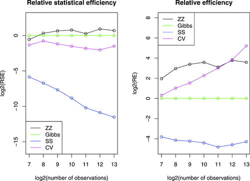
The use of subsampling methods for Bayesian variable selection problems is a recently emerging area (Song et al. 2020; Buchholz, Ahfock, and Richardson 2019). One of the attractions of PDMP samplers is that they can be implemented in a way where they only access a small subset of data at each iteration, while still targeting the true posterior. We now investigate how these ideas work in the variable selection problem, by comparing the efficiency of three implementations of ZigZag with that of the Gibbs sampler, and see how this depends on the number of observations. These are ZigZag using the full data, ZigZag using subsampling with a global bound, and ZigZag with subsampling control variates (see Bierkens, Fearnhead, and Roberts 2019, for details of both subsampling approaches).

Standard application of control variates requires calculation of the gradient at a reference point using the full likelihood. Due to the trans-dimensional nature of variable selection problems, a full gradient calculation is not well defined. For this reason we choose to make use of control variates defined for a fixed model $\mathcal{M}$ where the gradient is well defined. These control variates are only used when the sampler is in this model. For certain problems, such as generalized linear models, an O(n) initial calculation relating to the likelihood can be reused to define control variates for multiple models with certain parameters set to zero. See the supplementary material for more details.

Results are shown in Figure 2. In this simulation we take the independent prior ${\theta }_j\sim \frac{1}{15}\mathcal{N}(0,10)+(1-\frac{1}{15}){\delta }_0$, favoring models with a single selected variable. Despite our simplistic implementation, these results indicate that Zig-Zag with control variates is becoming increasingly efficient relative to Zig-Zag using the full dataset as the number of samples increases. Furthermore we see evidence of super-efficiency—whilst the computational cost per ESS of the Gibbs sampler is expected to be linear in the number of observations, the relative efficiency plots suggest that this is sublinear for ZigZag with control variates.

Fig. 2 Log-log plots of efficiency, relative to the Gibbs sampler, of different samplers as we vary the number of observations. Plotted are the relative efficiencies for the posterior mean conditional on model ${\mathcal{M}}^{*}$ where ${\mathcal{M}}^{*}$ corresponds to the true data generated model. The dataset was generated with a 15-dimensional regression parameter $\mathit{\theta }=(1,1,0,0,\dots ,0)$. The methods run are the Zig-Zag applied to the full dataset (zz, black), Zig-Zag with subsampling using global bounds (ss, blue), Zig-Zag with control variates (cv, magenta) and Gibbs sampling (Gibbs, green). All methods were initialized at the location of the control variate. Methods were given the same computational budget, for details see the supplementary materials.

5.2 Robust Regression

As mentioned in the introduction, a common approach to Bayesian variable selection is to use continuous spike-and-slab priors for each parameter rather than try to sample from the joint posterior of model and parameters. Such an approach is attractive as it enables standard gradient-based samplers, such as Hamiltonian Monte Carlo, to be used. We now compare such an approach, implemented with the popular Stan software (Carpenter et al. 2017), to our PDMP samplers. Our aim is to both investigate the computational efficiencies of the two approaches and to show the differences in posterior that we obtain from these different types of prior. Our comparison is based on a robust linear regression model.

In particular, we model the errors in our linear regression model as a mixture of normals with different variances. Thus, $$\begin{array}{c}\mathit{Y}=\sum _{i=1}^d{\mathit{X}}_j{\theta }_j+ϵ,\\ ϵ\sim \frac{1}{2}\mathrm{N}(0,1)+\frac{1}{2}\mathrm{N}(0,{10}^2).\end{array}$$

The continuous variable selection prior we consider is the regularized horseshoe (Piironen and Vehtari 2017a, 2017b) $$\begin{array}{c}{\theta }_j\sim N(0,{\tau }^2{\tilde{\lambda }}_j),\\ {\tilde{\lambda }}_j=\frac{c^2{\lambda }_j}{c^2+{\tau }^2{\lambda }_j},\\ {\lambda }_j\sim C^{+}(0,1)\end{array}$$for $j=1,\dots ,d$ where $C^{+}(0,1)$ denotes the half-Cauchy distribution for the standard deviation λ_j. The regularized horseshoe is a variation of the horseshoe prior (Carvalho, Polson, and Scott 2010) that offers a continuous approximation of a Dirac spike and slab where the slab is a normal distribution with finite variance c². The hyperparameter τ controls the global shrinkage of the variables toward zero. In Carvalho, Polson, and Scott (2010) it was shown that for standard linear regression the optimal choice for a fixed value of τ is ${\tau }_0=\sigma \frac{d_0}{(d-d_0)\sqrt{n}}$ where d₀ is a the number of nonzero variables in the sparse model and σ is the noise variance. In line with this, we compare the regularized horseshoe prior with fixed hyperparameter ${\tau }_0=\frac{d_0}{(d-d_0)\sqrt{n}}$ against the spike-and-slab prior $${\theta }_j\sim \frac{d_0}{d}N(0,c^2)+\left(1-\frac{d_0}{d}\right){\delta }_0$$ for $j=1,\dots ,d$. MCMC for the model using a horseshoe prior was performed by Stan’s implementation of NUTS (Hoffman and Gelman 2014).

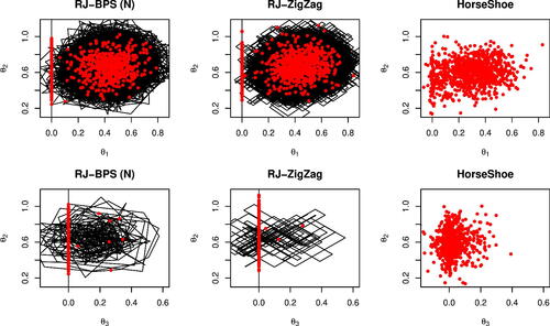
We first compare the variable selection dynamics for a simple model with d = 4 variables, n = 120 observations and regression parameter $\mathit{\theta }={(0.5,0.5,0,0)}^T$. The covariate values and residuals were generated as independent draws from a standard normal and the prior expected model size is set to $d_0=1$. Example output for the PDMP samplers and the Stan implementation is shown in Figure 3. The posteriors show the horseshoe prior replicating the effect of the spike-and-slab through shrinking the coefficients toward zero, but it is not able to give exact zeros.

Fig. 3 Dynamics of the samplers on a robust regression example with spike and slab or horseshoe prior. The top row shows the posterior for θ₁ and θ₂, bottom row shows the estimates for θ₂ and θ₃. The spike-and-slab distributions are sampled using the reversible jump PDMP samplers with reversible jump parameter 0.6 and refreshment for the BPS methods set to 0.5. All methods are shown with 10³ samples (red) and the PDMP dynamics are shown in black. Sampling with the Horseshoe prior was implemented in Stan using NUTS. Both Stan and PDMP methods were run for the same computing time. To aid visualization only the first 30% of the PDMP trajectories are shown.

We now compare the reversible jump PDMP methods in terms of their sampling efficiency for a higher dimensional problem. The dataset is generated for d = 200 variables and n = 100 observations with regression parameter $\mathit{\theta }={(2,2,2,\hspace{0.17em}2,0,0,0\dots 0)}^T$. The covariates for each observation were drawn from an AR(1) process with lag-1 correlation of 0.5. The residuals were generated from a standard Cauchy distribution.

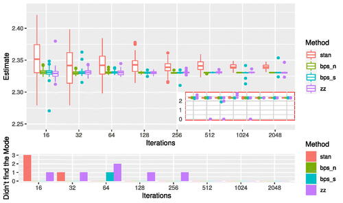
We ran Stan with the default settings for a burnin of 1000 iterations and then for 16, 32, 64,…, 2048 iterations. We ran the reversible jump PDMP samplers for the same wall clock time for both burnin and subsequent iterations. The experiment was repeated 50 times and the resulting boxplots of the posterior mean of θ₁ are shown in Figure 4. For the same computational budget, the reversible jump PDMP methods are able to attain better performance as can be seen by the lower Monte Carlo variability of their estimates. However, it is also apparent from this simulation that HMC is less susceptible to local modes, perhaps due to the horseshoe prior being continuous.

Fig. 4 Sampling efficiency for reversible jump PDMP versus Stan for the robust regression example. The PDMP samplers are ZigZag (zz), Bouncy Particle Sample with normally distributed velocities (bps_n) and with velocities distributed uniformly on the sphere (bps_s). The top figure shows boxplots of the posterior mean of θ₁ for increasing computational budget, with outliers from the sampler removed for visualization purposes. These removed outliers correspond to times that the sampler has become stuck in a local mode where ${\theta }_1=0$. The subplot shows the full results including outliers from the samplers. The Stan sampler is sampling from a different posterior to the PDMP methods, and this is seen in the estimates converging to slightly different values; but Monte Carlo efficiency can be assessed by comparing the variability of the estimates. The bottom figure shows the number of times that the samplers did not find the global mode.

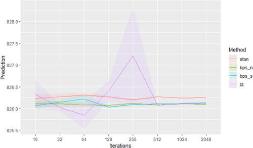
The predictive abilities of the methods are compared in Figure 5. Here an additional n = 100 observations were drawn from the same model and these were used as a hold-out dataset to validate the posterior predictive ability. The predictive ability is defined in terms of the Monte Carlo estimate of the mean square prediction performance $\frac{1}{100}{\sum }_{i=1}^{100}{(y_i-{\mathit{x}}_i^T\mathit{\theta })}^2$ where $\mathit{\theta }$ is replaced by the samples generated by either Stan or samples given by a discretization of time for the reversible jump PDMP samplers. The reversible jump PDMP samplers all give the same predictive performance for large iteration numbers while Stan, which uses a horseshoe prior, performs slightly worse.

Fig. 5 Predictive ability of reversible jump PDMP versus Stan for the robust regression example. The PDMP samplers are ZigZag (zz), Bouncy Particle Sample with normally distributed velocities (bps_n) and with velocities distributed uniformly on the sphere (bps_s). The predictive ability is measured by Monte Carlo estimates of the mean square predictive performance.

6 Discussion

We have shown how PDMP samplers can be extended so that they can sample from the joint posterior over model and parameters in variable selection problems. There are a number of open challenges that stem from this work. As with any MCMC algorithm, the reversible jump PDMP samplers have tuning parameters. The additional tuning parameters are the probabilities of moving between models when parameters hit zero. As a default, we recommend setting these probabilities all to the same value, and our simulation results were based on choosing this value after empirically evaluating the performance of the samplers on one simple problem. Whilst the samplers mixed well, it is likely that better mixing could be achieved if more informed choices of tuning parameters were made, and theory for guiding such choices is needed (e.g., see Sherlock and Thiery 2020, for theory on choosing the refresh rate of the Bouncy Particle Sampler).

The form of our reversible jump PDMP samplers is based on particular features of the variable selection problem. In other model choice settings, different trans-dimensional moves may be needed. The theory we developed should be able to be adapted to give rules for choosing rates of such moves. For example, in the case of sampling from mixture models one could introduce moves that remove a component when that component’s weight hits zero; and when we add a component we simulate new values for the component parameters from the prior. An advantage of such a construction would be that the rate of adding or removing components would not depend on the likelihood. Also our trans-dimensional moves are reversible, that is they balance probability flow from model i to model j by the flow of probability from model j to model i—it would be interesting to see if nonreversible trans-dimensional moves could be constructed.

It is likely that the reversible jump PDMP samplers will still struggle in situations where the posterior is multi-modal with well separated modes. For such cases it would be interesting to try and incorporate ideas such as tempering (Marinari and Parisi 1992) to allow for better mixing across modes. Also better mixing may be possible if we could introduce non-reversibility into exploring models, as in Power and Goldman (2019) and Gagnon and Maire (2020), though it is difficult to see how to incorporate lifting ideas that introduce such non-reversibility to our samplers. Finally, whilst we have considered only models with a finite number of variables, we believe the theory and PDMPs would extend to models with a countable number of variables, such as for polynomial regression. The challenge in using such PDMPs will be efficiently sampling when new variables are introduced into the model. If the rate at which each variable is added is simple and we can analytically calculate the sum of these rates, then this should be possible by simulating when a variable is added with a rate equal to this sum. At each such event we then simulate which variable to add.

Supplementary Materials

The supplementary material contains all proofs; results of empirical investigation of tuning parameters; additional results for the logistic regression model; details of implementations of the algorithms for the examples; and pseudo-code for the reversible-jump ZigZag algorithm.

Additional information

Funding

This research was supported by EPSRC grants EP/R018561 and EP/R034710.

References

- Bierkens, J., Bouchard-Côté, A., Doucet, A., Duncan, A. B., Fearnhead, P., Lienart, T., Roberts, G. O., and Vollmer, S. J. (2018), “Piecewise Deterministic Markov Processes for Scalable Monte Carlo on Restricted Domains,” Statistics & Probability Letters, 136, 148–154.
- Bierkens, J., Fearnhead, P., and Roberts, G. (2019), “The zig-zag Process and Super-Efficient Sampling for Bayesian Analysis of Big Data,” The Annals of Statistics, 47, 1288–1320. DOI: 10.1214/18-AOS1715.
- Bierkens, J., Grazzi, S., Kamatani, K., and Roberts, G. (2020), “The Boomerang Sampler,” in International Conference on Machine Learning, PMLR, pp. 908–918.
- Bierkens, J., Grazzi, S., van der Meulen, F., and Schauer, M. (2021), “Sticky PDMP Samplers for Sparse and Local Inference Problems,” arXiv:2103.08478.
- Bierkens, J., and Roberts, G. (2017), “A Piecewise Deterministic Scaling Limit of Lifted Metropolis–Hastings in the Curie–Weiss Model,” The Annals of Applied Probability, 27, 846–882. DOI: 10.1214/16-AAP1217.
- Bottolo, L., and Richardson, S. (2010), “Evolutionary Stochastic Search for Bayesian Model Exploration,” Bayesian Analysis, 5, 583–618. DOI: 10.1214/10-BA523.
- Bouchard-Côté, A., Vollmer, S. J., and Doucet, A. (2018), “The Bouncy Particle Sampler: A Nonreversible Rejection-Free Markov Chain Monte Carlo method,” Journal of the American Statistical Association, 113, 855–867. DOI: 10.1080/01621459.2017.1294075.
- Buchholz, A., Ahfock, D., and Richardson, S. (2019), “Distributed Computation for Marginal Likelihood based Model Choice,” arXiv.1910.04672.
- Carpenter, B., Gelman, A., Hoffman, M. D., Lee, D., Goodrich, B., Betancourt, M., Brubaker, M., Guo, J., Li, P., and Riddell, A. (2017), “Stan: A Probabilistic Programming Language,” Journal of Statistical Software, 76, 1–32. DOI: 10.18637/jss.v076.i01.
- Carvalho, C. M., Polson, N. G., and Scott, J. G. (2010), “The Horseshoe Estimator for Sparse Signals,” Biometrika, 97, 465–480. DOI: 10.1093/biomet/asq017.
- Chevallier, A., Fearnhead, P., and Sutton, M. (2020), “Reversible Jump PDMP Samplers for Variable Selection,” arXiv:2010.11771.
- Davis, M. (1993), Markov Models and Optimization, New York: Chapman Hall.
- de Valpine, P., Turek, D., Paciorek, C., Anderson-Bergman, C., Temple Lang, D., and Bodik, R. (2017), “Programming with Models: Writing Statistical Algorithms for General Model Structures with NIMBLE,” Journal of Computational and Graphical Statistics, 26, 403–413. DOI: 10.1080/10618600.2016.1172487.
- Diaconis, P., Holmes, S., and Neal, R. M. (2000), “Analysis of a Nonreversible Markov Chain Sampler,” Annals of Applied Probability, 10, 726–752.
- Fearnhead, P., Bierkens, J., Pollock, M., and Roberts, G. O. (2018), “Piecewise Deterministic Markov Processes for Continuous-Time Monte Carlo,” Statistical Science, 33, 386–412. DOI: 10.1214/18-STS648.
- Gagnon, P., and Maire, F. (2020), “Lifted Samplers for Partially Ordered Discrete State-Spaces,” arXiv:2003.05492.
- George, E. I., and McCulloch, R. E. (1993), “Variable Selection via Gibbs Sampling,” Journal of the American Statistical Association, 88, 881–889. DOI: 10.1080/01621459.1993.10476353.
- Geweke, J. (1996), “Variable Selection and Model Comparison in Regression,” in Bayesian Statistics 5, pp. 609–620, Oxford: Oxford University Press.
- Goldman, J. V., Sell, T., and Singh, S. S. (2021), “Gradient-based Markov Chain Monte Carlo for Bayesian Inference with Non-differentiable Priors,” Journal of the American Statistical Association, 1–12. DOI: 10.1080/01621459.2021.1909600.
- Green, P. J. (1995), “Reversible Jump Markov Chain Monte Carlo Computation and Bayesian Model Determination,” Biometrika, 82, 711–732. DOI: 10.1093/biomet/82.4.711.
- Grenander, U., and Miller, M. I. (1994), “Representations of Knowledge in Complex Systems,” Journal of the Royal Statistical Society, Series B, 56, 549–581. DOI: 10.1111/j.2517-6161.1994.tb02000.x.
- Hoffman, M. D., and Gelman, A. (2014), “The No-U-Turn Sampler: Adaptively Setting Path Lengths in Hamiltonian Monte Carlo,” Journal of Machine Learning Research, 15, 1593–1623.
- Ishwaran, H., and Rao, J. S. (2005), “Spike and Slab Variable Selection: Frequentist and Bayesian Strategies,” The Annals of Statistics, 33, 730–773. DOI: 10.1214/009053604000001147.
- Kuo, L., and Mallick, B. K. (1998), “Variable Selection for Regression Models,” Sankhya Series B 60, 65–81.
- Marinari, E., and Parisi, G. (1992), “Simulated Tempering: A New Monte Carlo Scheme,” EPL (Europhysics Letters), 19, 451. DOI: 10.1209/0295-5075/19/6/002.
- Markovic, J., and Sepehri, A. (2018), “Bouncy Hybrid Sampler as a Unifying Device,” arXiv:1802.04366 .
- Michel, M., Durmus, A., and Sénécal, S. (2020), “Forward Event-Chain Monte Carlo: Fast Sampling by Randomness Control in Irreversible Markov Chains,” Journal of Computational and Graphical Statistics, 29, 689–702. DOI: 10.1080/10618600.2020.1750417.
- Michel, M., Kapfer, S. C., and Krauth, W. (2014), “Generalized Event-Chain Monte Carlo: Constructing Rejection-Free Global-Balance Algorithms from Infinitesimal Steps,” The Journal of Chemical Physics, 140, 054116. DOI: 10.1063/1.4863991.
- Mitchell, T. J., and Beauchamp, J. J. (1988), “Bayesian Variable Selection in Linear Regression,” Journal of the American Statistical Association, 83, 1023–1032. DOI: 10.1080/01621459.1988.10478694.
- Neal, R. M. (2011), “MCMC using Hamiltonian Dynamics,” in Handbook of Markov Chain Monte Carlo, eds. A. Brooks, A. Gelman, G. L. Jones and X. Meng, Boca Raton, FL: pp. 113–162, Chapman & Hall/CRC.
- Peters, E. A., and de With, G. (2012), “Rejection-Free Monte Carlo Sampling for General Potentials,” Physical Review E, 85, 026703. DOI: 10.1103/PhysRevE.85.026703.
- Phillips, D. B., and Smith, A. F. (1996), “Bayesian Model Comparison via Jump Diffusions,” in Markov Chain Monte Carlo in Practice, eds. W. R. Gilks, S. Richardson and D. Spiegelhalter, pp. 215–240, Boca Raton, FL: Chapman & Hall, CRC.
- Piironen, J., and Vehtari, A. (2017a), “On the Hyperprior Choice for the Global Shrinkage Parameter in the Horseshoe Prior,” Vol. 54 of Proceedings of Machine Learning Research, PMLR, pp. 905–913.
- Piironen, J., and Vehtari, A. (2017b), “Sparsity Information and Regularization in the Horseshoe and other Shrinkage Priors,” Electronic Journal of Statistics, 11, 5018–5051.
- Polson, N. G., Scott, J. G., and Windle, J. (2013), “Bayesian Inference for Logistic Models using Pólya–Gamma Latent Variables,” Journal of the American Statistical Association, 108, 1339–1349. DOI: 10.1080/01621459.2013.829001.
- Power, S., and Goldman, J. V. (2019), “Accelerated Sampling on Discrete Spaces with Non-reversible Markov Processes,” arXiv:1912.04681.
- Sherlock, C., and Thiery, A. H. (2020), “A Discrete Bouncy Particle Sampler,” Biometrika (to appear). DOI: 10.1093/biomet/asab013.
- Smith, M., and Kohn, R. (1996), “Nonparametric Regression using Bayesian Variable Selection,” Journal of Econometrics, 75, 317–343. DOI: 10.1016/0304-4076(95)01763-1.
- Song, Q., Sun, Y., Ye, M., and Liang, F. (2020), “Extended Stochastic Gradient Markov Chain Monte Carlo for Large-Scale Bayesian Variable Selection,” Biometrika, 107, 997–1004.
- Stephens, M. (2000), “Bayesian Analysis of Mixture Models with an Unknown Number of Components-an Alternative to Reversible Jump Methods,” Annals of Statistics, 28, 40–74.
- Vanetti, P., Bouchard-Côté, A., Deligiannidis, G., and Doucet, A. (2017), “Piecewise-Deterministic Markov Chain Monte Carlo,” arXiv:1707.05296.
- Wang, S., Nan, B., Rosset, S., and Zhu, J. (2011), “Random Lasso,” Annals of Applied Statistics, 5, 468–485.
- Wu, C., and Robert, C. P. (2020), “Coordinate Sampler: A Non-reversible Gibbs-like MCMC Sampler,” Statistics and Computing, 30, 721–730. DOI: 10.1007/s11222-019-09913-w.
- Yang, Y., Wainwright, M. J., and Jordan, M. I. (2016), “On the Computational Complexity of High-Dimensional Bayesian Variable Selection,” The Annals of Statistics, 44, 2497–2532. DOI: 10.1214/15-AOS1417.
- Zanella, G., and Roberts, G. (2019), “Scalable Importance Tempering and Bayesian Variable Selection,” Journal of the Royal Statistical Society, Series B, 81, 489–517. DOI: 10.1111/rssb.12316.