Partially Linear Additive Regression with a General Hilbertian Response

ABSTRACT

In this article we develop semiparametric regression techniques for fitting partially linear additive models. The methods are for a general Hilbert-space-valued response. They use a powerful technique of additive regression in profiling out the additive nonparametric components of the models, which necessarily involves additive regression of the nonadditive effects of covariates. We show that the estimators of the parametric components are $\sqrt{n}$-consistent and asymptotically Gaussian under weak conditions. We also prove that the estimators of the nonparametric components, which are random elements taking values in a space of Hilbert-space-valued maps, achieve the univariate rate of convergence regardless of the dimension of covariates. We present some numerical evidence for the success of the proposed method and discuss real data applications. Supplementary materials for this article are available online.

KEYWORDS:

• Additive models
• Hilbert-space-valued data
• Partially linear models
• Profiling
• Projection operators

1 Introduction

We study useful semiparametric regression techniques that can be used for analyzing a finite or infinite dimensional response variable. The response variable takes values in a general separable Hilbert space. The model consists of a parametric and a nonparametric part. The parametric part is linear in a covariate (predictor) vector, say $\mathbf{X}={(X_1,\dots ,X_p)}^{\top }$ for $p\ge 1$, and the nonparametric part is to model the effect of another covariate vector, say $\mathbf{Z}={(Z_1,\dots ,Z_d)}^{\top }$ for $d\ge 1$. To avoid the curse of dimensionality in estimating the nonparametric part, it is assumed that the nonparametric effect is additive in Z, that is, it adds the unknown nonparametric effects of the individual covariates Z_k. We consider two scenarios for X. One is that both X_j and Z_k are real-valued, and the other that X_j take values in the Hilbert space where the response variable takes values while Z_k are real-valued. The new techniques are important extensions of the partially linear additive regression for scalar responses coupled with scalar covariates studied by Yu, Mammen, and Park (2011). In this article, we develop powerful techniques of estimating the models and provide sound theory that supports the methodology.

Our framework of Hilbert-space-valued (henceforth, Hilbertian) responses can be specialized to various data types. Its coverage is broad enough to include random variables, random vectors, random functions, random densities, compositional random vectors, infinite sequence random vectors, and compositional random functions, etc. All these types are commonly encountered in today’s data environments. The present work also provides a base toward semiparametric regression for other response spaces, such as Riemannian manifolds and Lie groups, along the way paved by Lin, Müller, and Park (2022). The latter work pioneered a link connecting additive regression for manifold-valued responses to Hilbertian additive regression (Jeon and Park 2020) via Riemannian logarithmic map. Despite its importance, semiparametric regression with Hilbertian responses remains unexplored. To the best of our knowledge, this is the first attempt to study a semiparametric regression model for general Hilbertian responses.

We prove that our estimators of the parametric effects of X_j are $\sqrt{n}$-consistent in case X_j are real-valued. We also derive the joint asymptotic distribution of the parametric estimators. For Hilbertian X_j, we show that the corresponding parametric estimators are still $\sqrt{n}$-consistent if the Hilbert space where X_j take values is of finite-dimension, while they achieve a slightly slower rate if the Hilbert space is of infinite-dimension. Furthermore, we show that our methodology of estimating the nonparametric effect of the covariate Z is free from the curse of dimensionality, that is, affords a univariate rate of convergence regardless of the dimension of Z. This is in contrast with the partially linear modeling approach that does not have additivity structure in the nonparametric part. The latter suffers from the dimensionality problem. Not only the nonparametric part, our approach also improves the estimation of the parametric part. Indeed, we demonstrate, theoretically and numerically, that using additivity structure in the nonparametric part leads to efficiency gain in the estimation of the parametric part. It turns out that the gain is larger if $\mathrm{E}(X_j|\mathbf{Z}=·)$ are farther from being additive.

The present work is not considered a direct extension of Yu, Mammen, and Park (2011). Dealing with a general Hilbert space, instead of the conventional $\mathbb{R}$, as the space of the values of the response variable, needs a number of innovations in developing relevant methodology and theory. In case X_j takes values in $\mathbb{R}$, the theory requires to assess the stochastic magnitude of terms of the form $n^{-1}{\sum }_{i=1}^n{\mathbf{U}}_i·\widehat{g}(Z_{ij})$ for some ${\mathbf{U}}_i$, which is a known function of $({\mathbf{X}}_i,{\mathbf{Z}}_i)$, and for some stochastic (random) map $\widehat{g}$, which is a random element taking values in the space of Hilbertian maps $g:S\to \mathcal{H}$ for a Hilbert space $\mathcal{H}$ and a compact subset S of $\mathbb{R}$. The usual way of analyzing such a $\widehat{g}$-weighted average is to consider a large set $\mathcal{G}$ to which $\widehat{g}$ belongs with a high probability, and then derive the maximal stochastic size of $n^{-1}{\sum }_{i=1}^n{\mathbf{U}}_i·g(Z_{ij})$ over $g\in \mathcal{G}$ using an entropy bound for the set $\mathcal{G}$. The set $\mathcal{G}$ embodies Hilbertian maps $g:S\to \mathcal{H}$. In case $\mathcal{H}$ is finite-dimensional as Euclidean spaces, the entropy of $\mathcal{G}$ is finite although the dimension of $\mathcal{G}$ may be infinite, particularly when $\mathcal{G}$ is a class of nonparametric maps g. In case $\mathcal{H}$ is infinite-dimensional, however, the entropy of $\mathcal{G}$ is infinite so that it is not feasible to apply the empirical process theory directly to the $\widehat{g}$-weighted average. To resolve this difficulty we take the Hilbertian norm of the $\widehat{g}$-weighted average, and convert its maximal stochastic size to that of a $\tilde{g}$-weighted average where $\tilde{g}$ is a stochastic map from S to $\mathbb{R}$. The conversion with the associated calculation of the sizes of various stochastic terms is one of the challenges we tackle in this article. For Hilbertian X_j taking values in $\mathcal{H}$, however, a similar idea leads to dealing with $n^{-1}{\sum }_{i=1}^n\widehat{\eta }({\mathbf{V}}_i,Z_{ij})$, where ${\mathbf{V}}_i$ is an $\mathcal{H}$-valued function of $({\mathbf{X}}_i,{\mathbf{Z}}_i)$ and $\widehat{\eta }$ is a stochastic map from $\mathcal{H}\times S$ to $\mathbb{R}$. It turns out that the class embodying the latter stochastic map with a high probability does not necessarily have a finite entropy. Thus, the case of Hilbertian X_j needs a different treatment, which is another difficulty we resolve in this work.

Our proposals are related to Jeon and Park (2020), which developed a smooth backfitting technique for additive regression with Hilbertian responses. The latter, however, is for additive models without parametric component X, and for additive regression of additive effect, that is, for estimating the “assumed” additive effect of Z. It does not cover cases where the additivity model assumption is violated in additive regression. In contrast, our work is for models with linear effect of X in addition to the additive nonparametric effect of the covariate vector Z. Dealing with the additional linear effect necessarily involves additive regression of nonadditive effects. In this respect, our theory for additive regression is more general than the one in Jeon and Park (2020). Moreover, our modeling approach allows for discrete type covariates (ordinal or nominal), which arise in a variety of statistical problems.

In the case of a functional response, say $Y(·):\mathcal{T}\to \mathbb{R}$ for a domain $\mathcal{T}\subset {\mathbb{R}}^q$, which is a special case of Hilbetian response, one might think of applying a technique for scalar responses, such as the one in Yu, Mammen, and Park (2011), in a pointwise manner to Y(t) for each $t\in \mathcal{T}$ and combine the pointwise results $\widehat{Y}(t)$, to construct $\widehat{Y}(·)$. However, this naive approach is problematic since the resulting $\widehat{Y}(·)$ is not guaranteed to take values in the space where $Y(·)$ comes from. This is particularly the case when $Y(·)$ has constraints, for example, $Y(·)\ge 0$ and ${\int }_{\mathcal{T}}Y(t) dt=1$, like a random density. Similarly, for a compositional response $Y\equiv (Y_1,\dots ,Y_k)$ with $0<Y_j<1$ and ${\sum }_{j=1}^k{Y}_j\equiv 1$, component-wise regression with Y_j for each j does not give simplex-valued $\widehat{Y}$ as a whole. Our approach does not have these drawbacks when specialized to functional and compositional data since it applies directly to the observations of functional $Y(·)$ and of compositional vector Y, respectively, as data objects.

A few past works on semiparametric regression for real-valued responses include the estimation of partially linear models without additivity structure in the nonparametric part (Bhattacharya and Zhao 1997; Liang 2006), and of partially linear additive models (Opsomer and Ruppert 1999; Liang et al. 2008; Yu, Mammen, and Park 2011; Lee, Han, and Park 2018). Among the latter four studying partially linear additive models, Opsomer and Ruppert (1999) and Liang et al. (2008) employed the ordinary backfitting technique (Buja, Hastie, and Tibshirani 1989) to estimate the additive nonparametric part, while Yu, Mammen, and Park (2011) and Lee, Han, and Park (2018) used the smooth backfitting technique (Mammen, Linton, and Nielsen 1999). The smooth backfitting method has been proved to be successful in various structured nonparametric models under weak conditions (Yu, Park, and Mammen 2008; Linton, Sperlich, and van Keilegom 2008; Lee, Mammen, and Park 2010, 2012; Zhang, Park, and Wang 2013; Bissantz et al. 2016; Han and Park 2018; Han, Müller, and Park 2020). On the contrary, the ordinary backfitting is known to work under stronger conditions on covariates (Opsomer and Ruppert 1997).

2 Additive Regression

Our approach to the semiparametric regression requires the estimation of “best” approximations of $\mathrm{E}(\mathbf{W}|\mathbf{Z}=·)$ for W being a general Hilbertian random element, or a real-valued random variable in the respective spaces of “additive” maps. This section is devoted to characterizing the best approximations and their estimation. We assume that Z is supported on ${[0,1]}^d$.

2.1 Projection on Additive Function Space

We consider a general separable Hilbert space, denoted by $\mathbb{H}$. Euclidean spaces, L² spaces, Bayes-Hilbert spaces and simplices are special cases of $\mathbb{H}$. Here and below, we denote $\mathbb{H}$-valued maps, random elements taking values in $\mathbb{H}$ and their values in $\mathbb{H}$, by bold-faced symbols. Note that we also use bold-faced symbols to denote random vectors and their realizations. Let $\mathbf{0}$ be the zero vector in $\mathbb{H},〈·,·〉$ the inner product of $\mathbb{H}$ and $\left|\right|·\left|\right|$ the associated norm. We denote by $\oplus$ and $\odot$ the operations of vector addition and of scalar multiplication in $\mathbb{H}$, respectively. Let $\ominus$ denote the subtraction operation defined by $\mathbf{a} \ominus \mathbf{b}=\mathbf{a} \oplus (-1)\odot \mathbf{b}$.

We let ${\mathcal{H}}_{\text{add}}(\mathbb{H})$ denote the space of additive maps $\mathbf{g}:{[0,1]}^d\to \mathbb{H}$ such that $\mathrm{E}(||\mathbf{g}(\mathbf{Z})|{|}^2)<\infty$ and $\mathbf{g}(\mathbf{z})={\mathbf{g}}_1(z_1) \oplus \cdots \oplus {\mathbf{g}}_d(z_d)$ for some ${\mathbf{g}}_j:[0,1]\to \mathbb{H}$. For a random element W taking values in $\mathbb{H}$ with $\mathrm{E}(|\left|\mathbf{W}\right|{|}^2)<\infty$, let ${\mathbf{m}}_{\mathbf{W},+}={\mathbf{m}}_{\mathbf{W},1} \oplus \cdots \oplus {\mathbf{m}}_{\mathbf{W},d}$ denote the projection of the mean regression map ${\mathbf{m}}_{\mathbf{W}}:=\mathrm{E}(\mathbf{W}|\mathbf{Z}=·)$ onto ${\mathcal{H}}_{\text{add}}(\mathbb{H})$. That is, (2.1) $${\mathbf{m}}_{\mathbf{W},+}=\text{arg} {\min }_{{\mathbf{g}}_{+}\in {\mathcal{H}}_{\text{add}}(\mathbb{H})} {\int }_{{[0,1]}^d}{\Vert {\mathbf{m}}_{\mathbf{W}}(\mathbf{z}) \ominus {\mathbf{g}}_{+}(\mathbf{z})\Vert }^{2}f(\mathbf{z}) d\mathbf{z},$$(2.1) where f is the joint density of Z. For the definition of the conditional expectation for Hilbertian W, we refer to Bosq (2000). The minimizer ${\mathbf{m}}_{\mathbf{W},+}$ with ${\mathbf{m}}_{\mathbf{W},+}(\mathbf{z})={\mathbf{m}}_{\mathbf{W},1}(z_1)\oplus \cdots \oplus {\mathbf{m}}_{\mathbf{W},d}(z_d)$ satisfies (2.2) $$\begin{array}{cc}\mathbf{0}\hfill & ={\int }_{{[0,1]}^{d-1}}\frac{f(\mathbf{z})}{f_j(z_j)}\odot \left({\mathbf{m}}_{\mathbf{W}}(\mathbf{z}) \ominus {\mathbf{m}}_{\mathbf{W},1}(z_1) \ominus \cdots \ominus {\mathbf{m}}_{\mathbf{W},d}(z_d)\right) d{\mathbf{z}}_{-j}\hfill \\ \hfill & =\mathrm{E}(\mathbf{W}|Z_j=z_j) \ominus \underset{k\ne j}{\oplus }{\int }_0^1\frac{f_{jk}(z_j,z_k)}{f_j(z_j)}\odot {\mathbf{m}}_{\mathbf{W},k}(z_k) d{z}_k \ominus {\mathbf{m}}_{\mathbf{W},j}(z_j)\hfill \end{array}$$(2.2) for each $1\le j\le d$ and for all z_j with $f_j(z_j)>0$. Here and below, ${\mathbf{z}}_{-j}$ for a d-vector z is $(z_1,\dots ,z_{j-1},z_{j+1},\dots ,z_d)$, and f_j and f_jk are the densities of Z_j and (Z_j, Z_k), respectively. The integrals in (2.2) are special cases of the so called “Bochner integral” (Jeon and Park 2020), the latter being for Banach-space-valued maps. From (2.2), we see that the additive map ${\mathbf{m}}_{\mathbf{W},+}$ is characterized as the solution of the following system of Hilbertian integral equations: (2.3) $$\begin{array}{cc}{\mathbf{m}}_{\mathbf{W},j}(z_j)\hfill & =\mathrm{E}(\mathbf{W}|Z_j=z_j)\ominus \underset{k\ne j}{\oplus }{\int }_0^1\frac{f_{jk}(z_j,z_k)}{f_j(z_j)}\odot {\mathbf{m}}_{\mathbf{W},k}(z_k) d{z}_k,\hfill \\ \hfill & \mathrm{\hspace{1em}}\mathrm{\hspace{1em}}1\le j\le d.\hfill \end{array}$$(2.3)

We note that (2.3) does not define a component tuple $({\mathbf{m}}_{\mathbf{W},j}:1\le j\le d)$, but only the sum of its entries, ${\mathbf{m}}_{\mathbf{W},+}={\mathbf{m}}_{\mathbf{W},1} \oplus \cdots \oplus {\mathbf{m}}_{\mathbf{W},d}$. Obviously, if $({\mathbf{m}}_{\mathbf{W},j}:1\le j\le d)$ satisfies (2.3), then $({\mathbf{m}}_{\mathbf{W},1} \ominus \mathbf{c},{\mathbf{m}}_{\mathbf{W},2} \oplus \mathbf{c},{\mathbf{m}}_{\mathbf{W},3},\dots ,{\mathbf{m}}_{\mathbf{W},d})$ also satisfies (2.3) for any constant $\mathbf{c}\in \mathbb{H}$. We also note that ${\mathbf{m}}_{\mathbf{W},+}\in {\mathcal{H}}_{\text{add}}(\mathbb{H})$ is different from the regression map ${\mathbf{m}}_{\mathbf{W}}$ unless ${\mathbf{m}}_{\mathbf{W}}$ belongs to ${\mathcal{H}}_{\text{add}}(\mathbb{H})$. Thus, the problem of estimating ${\mathbf{m}}_{\mathbf{W},+}$, which we present in Section 2.2, is different from that of estimating ${\mathbf{m}}_{\mathbf{W}}$ under the assumption ${\mathbf{m}}_{\mathbf{W}}\in {\mathcal{H}}_{\text{add}}(\mathbb{H})$, the latter having been studied by Jeon and Park (2020).

2.2 Estimation of Additive Projection

We now discuss the estimation of ${\mathbf{m}}_{\mathbf{W},+}$. The basic idea is to replace the marginal regression maps $\mathrm{E}(\mathbf{W}|Z_j=·)$ and the densities f_j and f_jk in (2.3) by the corresponding kernel estimators and then to solve the resulting system of equations. We note that our method requires the estimation of ${\mathbf{m}}_{X_j,+}$ for real-valued X_j and of ${\mathbf{m}}_{{\mathbf{X}}_j,+}$ for Hilbertian ${\mathbf{X}}_j$, as well. Below, we describe the method for W taking values in a general Hilbert space, since specialization to the case of random variables is immediate from the general treatment.

Suppose that we have n observations, $({\mathbf{Z}}_i,{\mathbf{W}}_i), 1\le i\le n$, with ${\mathbf{Z}}_i={(Z_{i1},\dots ,Z_{id})}^{\top }$. We estimate the marginal regression map ${\mathbf{M}}_{\mathbf{W},j}(z_j):=\mathrm{E}(\mathbf{W}|Z_j=z_j)$ for $z_j\in [0,1]$ by (2.4) $${\widehat{\mathbf{M}}}_{\mathbf{W},j}(z_j)={\widehat{f}}_j{(z_j)}^{-1}·n^{-1}\odot {\oplus }_{i=1}^n\left(K_{h_j}(z_j,Z_{ij})\odot {\mathbf{W}}_i\right),$$(2.4) where ${\widehat{f}}_j(z_j)=n^{-1}{\sum }_{i=1}^n{K}_{h_j}(z_j,Z_{ij})$ is a kernel estimator of f_j. We also estimate f_jk by ${\widehat{f}}_{jk}(z_j,z_k)=n^{-1}{\sum }_{i=1}^n{K}_{h_j}(z_j,Z_{ij})K_{h_k}(z_k,Z_{ik})$. Here and throughout the article, $K_h(·,·)$ is a normalized kernel function defined by $$K_h(u,v)=\frac{K_h(u-v)}{{\int }_0^1{K}_h(t-v) dt},\hspace{1em}u,v\in [0,1],$$ where h > 0 is the bandwidth, $K_h(w)=K(w/h)/h$ and $K(·)\ge 0$ is the baseline kernel function. This type of normalized kernels have been used in the literature (Yu, Park, and Mammen 2008; Lee, Mammen, and Park 2010, 2012; Jeon and Park 2020). It has the property that ${\int }_0^1{K}_h(u,v) du=1$ for all $v\in [0,1]$, which gives ${\int }_0^1{\widehat{f}}_j(z_j) d{z}_j=1$ and ${\int }_0^1{\widehat{f}}_{jk}(z_j,z_k) d{z}_k={\widehat{f}}_j(z_j)$ for all $z_j\in [0,1]$. Plugging these estimators into (2.3) gives the following estimated system of Hilbertian integral equations: (2.5) $$\begin{array}{cc}{\widehat{\mathbf{m}}}_{\mathbf{W},j}(z_j)\hfill & ={\widehat{\mathbf{M}}}_{\mathbf{W},j}(z_j) \ominus \underset{k\ne j}{\oplus }{\int }_0^1\frac{{\widehat{f}}_{jk}(z_j,z_k)}{{\widehat{f}}_j(z_j)}\odot {\widehat{\mathbf{m}}}_{\mathbf{W},k}(z_k) d{z}_k,\hfill \\ \hfill & \mathrm{\hspace{1em}}\mathrm{\hspace{1em}}1\le j\le d.\hfill \end{array}$$(2.5)

In the supplement S.7, we will show that the system of equations (2.5)(2.5) $$\begin{array}{cc}{\widehat{\mathbf{m}}}_{\mathbf{W},j}(z_j)\hfill & ={\widehat{\mathbf{M}}}_{\mathbf{W},j}(z_j) \ominus \underset{k\ne j}{\oplus }{\int }_0^1\frac{{\widehat{f}}_{jk}(z_j,z_k)}{{\widehat{f}}_j(z_j)}\odot {\widehat{\mathbf{m}}}_{\mathbf{W},k}(z_k) d{z}_k,\hfill \\ \hfill & \mathrm{\hspace{1em}}\mathrm{\hspace{1em}}1\le j\le d.\hfill \end{array}$$(2.5) has a unique solution, which we denote by ${\widehat{\mathbf{m}}}_{\mathbf{W},+}$. Just like that the system of equations at (2.3) determines only ${\mathbf{m}}_{\mathbf{W},+}={\mathbf{m}}_{\mathbf{W},1} \oplus \cdots \oplus {\mathbf{m}}_{\mathbf{W},d}$, the Equation (2.5)(2.5) $$\begin{array}{cc}{\widehat{\mathbf{m}}}_{\mathbf{W},j}(z_j)\hfill & ={\widehat{\mathbf{M}}}_{\mathbf{W},j}(z_j) \ominus \underset{k\ne j}{\oplus }{\int }_0^1\frac{{\widehat{f}}_{jk}(z_j,z_k)}{{\widehat{f}}_j(z_j)}\odot {\widehat{\mathbf{m}}}_{\mathbf{W},k}(z_k) d{z}_k,\hfill \\ \hfill & \mathrm{\hspace{1em}}\mathrm{\hspace{1em}}1\le j\le d.\hfill \end{array}$$(2.5) by itself defines only ${\widehat{\mathbf{m}}}_{\mathbf{W},+}={\widehat{\mathbf{m}}}_{\mathbf{W},1} \oplus \cdots \oplus {\widehat{\mathbf{m}}}_{\mathbf{W},d}$, not individual components ${\widehat{\mathbf{m}}}_{\mathbf{W},j}$. The solution ${\widehat{\mathbf{m}}}_{\mathbf{W},+}$ does not have a closed form, but can be computed by iteration starting with an initial tuple $({\widehat{\mathbf{m}}}_{\mathbf{W},j}^{[0]}:1\le j\le d)$. We may simply take ${\widehat{\mathbf{m}}}_{\mathbf{W},j}^{[0]}\equiv \mathbf{0}$, for example. In the rth ($r\ge 1$) cycle of the iteration, we update ${\widehat{\mathbf{m}}}_{\mathbf{W},j}^{[r-1]}$ by (2.6) $$\begin{array}{cc}{\widehat{\mathbf{m}}}_{\mathbf{W},j}^{\left[r\right]}(z_j)\hfill & ={\widehat{\mathbf{M}}}_{\mathbf{W},j}(z_j) \ominus {\oplus }_{k=1}^{j-1}{\int }_0^1\frac{{\widehat{f}}_{jk}(z_j,z_k)}{{\widehat{f}}_j(z_j)}\odot {\widehat{\mathbf{m}}}_{\mathbf{W},k}^{\left[r\right]}(z_k) d{z}_k\hfill \\ \hfill & \mathrm{\hspace{1em}}\mathrm{\hspace{1em}} \ominus {\oplus }_{k=j+1}^d{\int }_0^1\frac{{\widehat{f}}_{jk}(z_j,z_k)}{{\widehat{f}}_j(z_j)}\odot {\widehat{\mathbf{m}}}_{\mathbf{W},k}^{[r-1]}(z_k) d{z}_k,\hfill \\ \hfill & \mathrm{\hspace{1em}}\mathrm{\hspace{1em}}1\le j\le d.\hfill \end{array}$$(2.6)

In the supplement S.7, we will show that ${\widehat{\mathbf{m}}}_{\mathbf{W},+}^{[r]}:={\widehat{\mathbf{m}}}_{\mathbf{W},1}^{[r]} \oplus \cdots \oplus {\widehat{\mathbf{m}}}_{\mathbf{W},d}^{[r]}$ converges to ${\widehat{\mathbf{m}}}_{\mathbf{W},+}$ as $r\to \infty$, see Proposition S.1. In the iteration, we can evaluate the Bochner integrals in (2.6) by the conventional Lebesgue integrals, provided that ${\widehat{\mathbf{m}}}_{\mathbf{W},j}^{[0]}$ are linear in ${\mathbf{W}}_i$, that is, ${\widehat{\mathbf{m}}}_{\mathbf{W},j}^{[0]}(z_j)=n^{-1}\odot {\oplus }_{i=1}^n(w_{ij}(z_j)\odot {\mathbf{W}}_i)$ for some real-valued functions $w_{ij}:[0,1]\to \mathbb{R}$. This is because the marginal ${\widehat{\mathbf{M}}}_{\mathbf{W},j}$ are also linear in ${\mathbf{W}}_i$ so that all the subsequent updates ${\widehat{\mathbf{m}}}_{\mathbf{W},j}^{[r]}$ for $r\ge 1$ are linear in ${\mathbf{W}}_i$. For a linear form $\mathbf{g}(u)=n^{-1}\odot {\oplus }_{i=1}^n{v}_i(u)\odot {\mathbf{W}}_i$ with real-valued weight functions $v_i:[0,1]\to \mathbb{R}$, it holds that $${\int }_0^1{\widehat{f}}_{jk}(z_j,u)\odot \mathbf{g}(u) du=n^{-1}\odot {\oplus }_{i=1}^n\left({\int }_0^1{v}_i(u)·{\widehat{f}}_{jk}(z_j,u) du\right)\odot {\mathbf{W}}_i,$$where the integral on the left side is in Bochner sense while the one on the right hand side is a Lebesgue integral.

The regression map ${\mathbf{m}}_{\mathbf{W}}$ is not assumed to be additive and thus estimating the additive map ${\mathbf{m}}_{\mathbf{W},+}$ is considered additive regression of nonadditive effect, which is different from additive regression of additive effect, developed by Mammen, Linton, and Nielsen (1999) and Jeon and Park (2020). The very core of the matter in the present case regarding additive regression is that, when we write $\mathbf{W}={\mathbf{m}}_{\mathbf{W},+}(\mathbf{Z}) \oplus {\mathit{\varrho }}_{\mathbf{W}}$ with ${\mathit{\varrho }}_{\mathbf{W}}:=\mathbf{W} \ominus {\mathbf{m}}_{\mathbf{W},+}(\mathbf{Z})$ as an error term, $\mathrm{E}({\mathit{\varrho }}_{\mathbf{W}}|\mathbf{Z})={\mathbf{m}}_{\mathbf{W}}(\mathbf{Z}) \ominus {\mathbf{m}}_{\mathbf{W},+}(\mathbf{Z})\ne \mathbf{0}$. Instead, by the definition of ${\mathbf{m}}_{\mathbf{W},+}$, we have $\mathrm{E}(〈{\mathit{\varrho }}_{\mathbf{W}},{\mathit{\delta }}_{+}(\mathbf{Z})〉)=0$ for all ${\mathit{\delta }}_{+}\in {\mathcal{H}}_{\text{add}}(\mathbb{H})$. This implies that, for all $1\le k\le d$ and for all ${\mathit{\delta }}_k:[0,1]\to \mathbb{H}$ with $\mathrm{E}(||{\mathit{\delta }}_k(Z_k)|{|}^2)<\infty$, $0=\mathrm{E}(〈{\mathit{\varrho }}_{\mathbf{W}},{\mathit{\delta }}_k(Z_k)〉)=\mathrm{E}(〈\mathrm{E}({\mathit{\varrho }}_{\mathbf{W}}|Z_k),{\mathit{\delta }}_k(Z_k)〉)$. This gives (2.7) $$\mathrm{E}({\mathit{\varrho }}_{\mathbf{W}}|Z_k)=\mathbf{0},\hspace{1em}1\le k\le d.$$(2.7)

We show that the latter is enough for the theory of ${\widehat{\mathbf{m}}}_{\mathbf{W},+}$, see the supplement S.7 for details.

3 Hilbertian PLAM with Scalar Covariates

We introduce a partially linear additive model for a $\mathbb{H}$-valued response Y and covariate vectors $\mathbf{X}\equiv {(X_1,\dots ,X_p)}^{\top }$ and $\mathbf{Z}\equiv {(Z_1,\dots ,Z_d)}^{\top }$ taking values in ${\mathbb{R}}^p$ and ${\mathbb{R}}^d$, respectively, and present a way of estimating the model. We allow the entries of X to be discrete (nominal or ordinal) while assuming that all entries of Z are of continuous type supported on $[0,1]$. We assume that $\mathrm{E}(X_j^2)<\infty$ for all $1\le j\le p$.

3.1 The Model

The Hilbertian partially linear additive model (HPLAM) is given by (3.1) $$\mathbf{Y}={\mathit{\beta }}_0 \oplus {\oplus }_{j=1}^p(X_j\odot {\mathit{\beta }}_j) \oplus {\oplus }_{k=1}^d{\mathbf{m}}_k(Z_k) \oplus \mathit{\epsilon },$$(3.1)

where ${\mathit{\beta }}_j$ are unknown constants in $\mathbb{H}$, ${\mathbf{m}}_k:[0,1]\to \mathbb{H}$ are unknown component maps with $\mathrm{E}(||{\mathbf{m}}_k(Z_k)|{|}^2)<\infty$ satisfying the constraints (3.2) $$\mathrm{E}({\mathbf{m}}_k(Z_k))=\mathbf{0},\hspace{1em}1\le k\le d,$$(3.2) and $\mathit{\epsilon }$ is a Hilbertian error term such that $\mathrm{E}(\mathit{\epsilon }|\mathbf{X},\mathbf{Z})=\mathbf{0}$ and $\mathrm{E}(|\left|\mathit{\epsilon }\right|{|}^2)<\infty$. Below, we give a proposition that establishes the identifiability of ${\mathit{\beta }}_j$ and ${\mathbf{m}}_k$ in the model (3.1). Let $P_{\mathbf{U}}$ denote the distribution of a random vector or element U. We make the following weak assumption.

(A0) The $P_{\mathbf{X},\mathbf{Z}}$ has a density with respect to the product measure $P_{\mathbf{X}}\otimes P_{\mathbf{Z}}$, which is bounded away from zero on the support of $P_{\mathbf{X},\mathbf{Z}}$. The marginal distribution $P_{\mathbf{Z}}$ has a density f with respect to the Lebesgue measure such that $f(\mathbf{z})>0$ for all $\mathbf{z}\in {[0,1]}^d$, and the support of $P_{\mathbf{X}}$ is not contained in a hyperplane in ${\mathbb{R}}^p$.

Proposition 3.1.

Let ${\mathit{\alpha }}_j\in \mathbb{H}$ for $0\le j\le p$ be Hilbertian constants and ${\mathbf{g}}_k:[0,1]\to \mathbb{H}$ for $1\le k\le d$ be Hilbertian maps with $\mathrm{E}(||{\mathbf{g}}_k(Z_k)|{|}^2)<\infty$ and $\mathrm{E}({\mathbf{g}}_k(Z_k))=\mathbf{0}$. Assume the condition (A0). Then, (3.3) $$\mathrm{E}\left({\Vert {\mathit{\alpha }}_0 \oplus {\oplus }_{j=1}^p(X_j\odot {\mathit{\alpha }}_j) \oplus {\oplus }_{k=1}^d{\mathbf{g}}_k(Z_k)\Vert }^2\right)=0$$(3.3) implies ${\mathit{\alpha }}_j=\mathbf{0}$ and ${\mathbf{g}}_k(Z_k)=\mathbf{0}$ a.s. for all $0\le j\le p$ and $1\le k\le d$.

A proof of Proposition 3.1 is given in the supplement S.1. With (3.2), we have ${\mathit{\beta }}_0=\mathrm{E}(\mathbf{Y}) \ominus {\oplus }_{j=1}^p\mathrm{E}(X_j)\odot {\mathit{\beta }}_j$, so that by plugging the expression into (3.1) we may rewrite the model (3.1) as $${\mathbf{Y}}^c={\oplus }_{j=1}^p{X}_j^c\odot {\mathit{\beta }}_j \oplus {\oplus }_{k=1}^d{\mathbf{m}}_k(Z_k) \oplus \mathit{\epsilon },$$where ${\mathbf{Y}}^c=\mathbf{Y} \ominus \mathrm{E}(\mathbf{Y})$ and $X_j^c=X_j-\mathrm{E}(X_j)$.

3.2 Estimation of Parametric Components

Here, we discuss the estimation of ${\mathit{\beta }}_j$ using the profiling technique (Severini and Wong 1992) in conjunction with the estimation of additive projections presented in Section 2.2. Let ${\mathbf{m}}_{+}={\mathbf{m}}_1 \oplus \cdots \oplus {\mathbf{m}}_d\in {\mathcal{H}}_{\text{add}}(\mathbb{H})$ and put $\mathit{\beta }={({\mathit{\beta }}_1,\dots ,{\mathit{\beta }}_p)}^{\top }$. Note that $\mathit{\beta }$ does not involve ${\mathit{\beta }}_0$. Then, under the model specification (3.1), (3.4) $$(\mathit{\beta },{\mathbf{m}}_{+})=\mathrm{}\underset{\mathbf{b}\in {\mathbb{H}}^p,{\mathbf{g}}_{+}\in {\mathcal{H}}_{\text{add}}(\mathbb{H})}{\text{argmin}}\mathrm{}\mathrm{E}(||{\mathbf{Y}}^c \ominus ({({\mathbf{X}}^c)}^{\top }\odot \mathbf{b}) \ominus {\mathbf{g}}_{+}(\mathbf{Z})|{|}^2),$$(3.4) where ${\mathbf{X}}^c={(X_1^c,\dots ,X_p^c)}^{\top }$. Here and below, ${\mathbf{c}}^{\top }\odot \mathbf{b}={\oplus }_{j=1}^p(c_j\odot {\mathbf{b}}_j)$ for $\mathbf{c}={(c_1,\dots ,c_p)}^{\top }\in {\mathbb{R}}^p$ and $\mathbf{b}={({\mathbf{b}}_1,\dots ,{\mathbf{b}}_p)}^{\top }\in {\mathbb{H}}^p$. Considering ${\mathbf{m}}_{{\mathbf{Y}}^c \ominus ({({\mathbf{X}}^c)}^{\top }\odot \mathbf{b}),+}$ for each $\mathbf{b}\in {\mathbb{H}}^p$, which solves the system of equations (2.3)(2.3) $$\begin{array}{cc}{\mathbf{m}}_{\mathbf{W},j}(z_j)\hfill & =\mathrm{E}(\mathbf{W}|Z_j=z_j)\ominus \underset{k\ne j}{\oplus }{\int }_0^1\frac{f_{jk}(z_j,z_k)}{f_j(z_j)}\odot {\mathbf{m}}_{\mathbf{W},k}(z_k) d{z}_k,\hfill \\ \hfill & \mathrm{\hspace{1em}}\mathrm{\hspace{1em}}1\le j\le d.\hfill \end{array}$$(2.3) with $\mathbf{W}={\mathbf{Y}}^c \ominus ({({\mathbf{X}}^c)}^{\top }\odot \mathbf{b})$ and noting that ${\mathbf{m}}_{{\mathbf{Y}}^c \ominus ({({\mathbf{X}}^c)}^{\top }\odot \mathit{\beta }),+}={\mathbf{m}}_{+}$, we get $$\mathit{\beta }=\underset{\mathbf{b}\in {\mathbb{H}}^p}{\text{argmin}} \mathrm{E}(||{\mathbf{Y}}^c \ominus ({({\mathbf{X}}^c)}^{\top }\odot \mathbf{b}) \ominus {\mathbf{m}}_{{\mathbf{Y}}^c \ominus ({({\mathbf{X}}^c)}^{\top }\odot \mathbf{b}),+}(\mathbf{Z})|{|}^2).$$

According to the arguments leading to Corollary S.1 in the supplement S.7, ${\mathbf{m}}_{\mathbf{W},+}$ is linear in W in the sense that ${\mathbf{m}}_{(\mathbf{W} \oplus \mathbf{W}\prime ),+}={\mathbf{m}}_{\mathbf{W},+} \oplus {\mathbf{m}}_{\mathbf{W}\prime ,+}$ and ${\mathbf{m}}_{\mathbf{W} \oplus \mathbf{c},+}={\mathbf{m}}_{\mathbf{W},+} \oplus \mathbf{c}$ for all Hilbertian variables $\mathbf{W},\mathbf{W}\prime$ and Hilbertian constant c. Also, it holds that ${\mathbf{m}}_{(W_1\odot {\mathbf{b}}_1) \oplus (W_2\odot {\mathbf{b}}_2),+}=(m_{W_1,+}\odot {\mathbf{b}}_1) \oplus (m_{W_2,+}\odot {\mathbf{b}}_2)$ for all Hilbertian constants ${\mathbf{b}}_j\in \mathbb{H}$ and random variables W_j. Thus, ${\mathbf{m}}_{{\mathbf{Y}}^c \ominus ({({\mathbf{X}}^c)}^{\top }\odot \mathbf{b}),+}={\mathbf{m}}_{{\mathbf{Y}}^c,+} \ominus (m_{{\mathbf{X}}^c,+}^{\top }\odot \mathbf{b})$. Furthermore, we also get $$\begin{array}{cc}{\mathbf{Y}}^c \ominus {\mathbf{m}}_{{\mathbf{Y}}^c,+}(\mathbf{Z})\hfill & =\left(\mathbf{Y} \ominus \mathrm{E}(\mathbf{Y})\right) \ominus \left({\mathbf{m}}_{\mathbf{Y},+}(\mathbf{Z}) \ominus \mathrm{E}(\mathbf{Y})\right)\hfill \\ \hfill & =\mathbf{Y} \ominus {\mathbf{m}}_{\mathbf{Y},+}(\mathbf{Z}),\hfill \end{array}$$and likewise ${\mathbf{X}}^c-m_{{\mathbf{X}}^c,+}(\mathbf{Z})=\mathbf{X}-m_{\mathbf{X},+}(\mathbf{Z})$. This gives (3.5) $$\mathit{\beta }=\underset{\mathbf{b}\in {\mathbb{H}}^p}{\text{argmin}} \mathrm{E}({\Vert (\mathbf{Y} \ominus {\mathbf{m}}_{\mathbf{Y},+}(\mathbf{Z})) \ominus {(\mathbf{X}-m_{\mathbf{X},+}(\mathbf{Z}))}^{\top }\mathrm{}\odot \mathbf{b}\Vert }^2).$$(3.5)

We estimate $\mathit{\beta }$ by minimizing an empirical version of the objective functional at (3.5). Define $${\tilde{X}}_{ij}=X_{ij}-{\widehat{m}}_{X_j,+}({\mathbf{Z}}_i),\hspace{1em}{\tilde{\mathbf{Y}}}_i={\mathbf{Y}}_i \ominus {\widehat{\mathbf{m}}}_{\mathbf{Y},+}({\mathbf{Z}}_i),$$where ${\widehat{m}}_{X_j,+}$ for $1\le j\le p$ and ${\widehat{\mathbf{m}}}_{\mathbf{Y},+}$, respectively, are the solutions of (2.5) for $\mathbf{W}=X_j$ and $\mathbf{W}=\mathbf{Y}$. Put ${\widehat{m}}_{\mathbf{X},+}={({\widehat{m}}_{X_1,+},\dots ,{\widehat{m}}_{X_p,+})}^{\top }$. Then, ${\tilde{\mathbf{X}}}_i:={({\tilde{X}}_{i1},\dots ,{\tilde{X}}_{ip})}^{\top }={\mathbf{X}}_i-{\widehat{m}}_{\mathbf{X},+}({\mathbf{Z}}_i)$. We propose to estimate $\mathit{\beta }$ by (3.6) $$\widehat{\mathit{\beta }}=\underset{\mathbf{b}\in {\mathbb{H}}^p}{\text{argmin}} n^{-1}\sum _{i=1}^n{\Vert {\tilde{\mathbf{Y}}}_i \ominus {\tilde{\mathbf{X}}}_i^{\top }\odot \mathbf{b}\Vert }^2.$$(3.6)

We present an explicit form of $\widehat{\mathit{\beta }}$ defined at (3.6). The Gâteaux derivative of the objective functional in (3.6) at $\widehat{\mathit{\beta }}$ to an arbitrary direction $\mathit{\delta }\in {\mathbb{H}}^p$ equals $$\begin{array}{cc}\hfill & -2 n^{-1}\sum _{i=1}^n〈{\tilde{\mathbf{X}}}_i^{\top }\odot \mathit{\delta }, {\tilde{\mathbf{Y}}}_i \ominus {\tilde{\mathbf{X}}}_i^{\top }\odot \widehat{\mathit{\beta }}〉\hfill \\ \hfill & \hspace{1em}=-2 n^{-1}\sum _{j=1}^p\sum _{i=1}^n〈{\mathit{\delta }}_j, {\tilde{X}}_{ij}\odot ({\tilde{\mathbf{Y}}}_i \ominus {\tilde{\mathbf{X}}}_i^{\top }\odot \widehat{\mathit{\beta }})〉\hfill \\ \hfill & \hspace{1em}=-2 n^{-1}\sum _{j=1}^p〈{\mathit{\delta }}_j, {\oplus }_{i=1}^n{\tilde{X}}_{ij}\odot ({\tilde{\mathbf{Y}}}_i \ominus {\tilde{\mathbf{X}}}_i^{\top }\odot \widehat{\mathit{\beta }})〉.\hfill \end{array}$$

Equating the above derivative with zero for all $\mathit{\delta }\in {\mathbb{H}}^p$ gives $${\oplus }_{i=1}^n{\tilde{X}}_{ij}\odot ({\tilde{\mathbf{Y}}}_i \ominus {\tilde{\mathbf{X}}}_i^{\top }\odot \widehat{\mathit{\beta }})=\mathbf{0},\hspace{1em}1\le j\le p.$$

From this we get that, whenever the p × p matrix ${\sum }_{i=1}^n{\tilde{\mathbf{X}}}_i{\tilde{\mathbf{X}}}_i^{\top }$ is invertible, (3.7) $$\widehat{\mathit{\beta }}={\left(\sum _{i=1}^n{\tilde{\mathbf{X}}}_i{\tilde{\mathbf{X}}}_i^{\top }\right)}^{-1}\odot \left({\oplus }_{i=1}^n{\tilde{\mathbf{X}}}_i\odot {\tilde{\mathbf{Y}}}_i\right),$$(3.7) where $\mathbf{c}\odot {\mathbf{v}}_0={(c_1\odot {\mathbf{v}}_0,\dots ,c_p\odot {\mathbf{v}}_0)}^{\top }\in {\mathbb{H}}^p$ for ${\mathbf{v}}_0\in \mathbb{H}$ and $\mathbf{c}={(c_1,\dots ,c_p)}^{\top }\in {\mathbb{R}}^p$, and $\mathbf{A}\odot \mathbf{b}={({\oplus }_{j=1}^p{a}_{1j}\odot {\mathbf{b}}_j,\dots ,{\oplus }_{j=1}^p{a}_{pj}\odot {\mathbf{b}}_j)}^{\top }$ for a p × p real matrix $\mathbf{A}=(a_{ij})$ and $\mathbf{b}={({\mathbf{b}}_1,\dots ,{\mathbf{b}}_p)}^{\top }\in {\mathbb{H}}^p$. With $\widehat{\mathit{\beta }}={({\widehat{\mathit{\beta }}}_1,\dots ,{\widehat{\mathit{\beta }}}_p)}^{\top }$ defined at (3.7) we estimate ${\mathit{\beta }}_0$ in the model (3.1) by $${\widehat{\mathit{\beta }}}_0=\overline{\mathbf{Y}} \ominus {\oplus }_{j=1}^p{\overline{X}}_j\odot {\widehat{\mathit{\beta }}}_j,$$ where ${\overline{X}}_j=n^{-1}{\sum }_{i=1}^n{X}_{ij}$ and $\overline{\mathbf{Y}}=n^{-1}\odot ({\oplus }_{i=1}^n{\mathbf{Y}}_i)$. In Section 7.1, we will show that $n^{-1}{\sum }_{i=1}^n{\tilde{\mathbf{X}}}_i{\tilde{\mathbf{X}}}_i^{\top }$ is invertible with probability tending to one and that $\widehat{\mathit{\beta }}$ is $\sqrt{n}$-consistent and $\sqrt{n}\odot (\widehat{\mathit{\beta }} \ominus \mathit{\beta })$ converges to a mean zero Gaussian random element taking values in $\mathbb{H}$.

3.3 Estimation of Nonparametric Components

We estimate ${\mathbf{m}}_{+}={\oplus }_{k=1}^d{\mathbf{m}}_k$ in the model (3.1) by ${\widehat{\mathbf{m}}}_{+}$, which solves the system of equations at (2.5) with ${\mathbf{W}}_i={\mathbf{Y}}_i \ominus {\widehat{\mathit{\beta }}}_0 \ominus ({\mathbf{X}}_i^{\top }\odot \widehat{\mathit{\beta }})$. From the linearity of ${\widehat{\mathbf{m}}}_{\mathbf{W},+}$ in $({\mathbf{W}}_1,\dots ,{\mathbf{W}}_n)$ (Corollary S.1 in the supplement S.7), it holds that ${\widehat{\mathbf{m}}}_{+}(\mathbf{z})={\widehat{\mathbf{m}}}_{\mathbf{Y},+}(\mathbf{z}) \ominus {\widehat{\mathit{\beta }}}_0 \ominus ({\widehat{m}}_{\mathbf{X},+}{(\mathbf{z})}^{\top }\odot \widehat{\mathit{\beta }})$, where ${\widehat{m}}_{\mathbf{X},+}(\mathbf{z})={({\widehat{m}}_{X_1,+}(\mathbf{z}),\dots ,{\widehat{m}}_{X_p,+}(\mathbf{z}))}^{\top }$. To estimate the individual component maps ${\mathbf{m}}_k$ satisfying the constraints $\mathrm{E}({\mathbf{m}}_k(Z_k))=\mathbf{0}$, we put the following constraints on ${\widehat{\mathbf{m}}}_k$: (3.8) $${\int }_0^1{\widehat{f}}_k(u)\odot {\widehat{\mathbf{m}}}_k(u) du=\mathbf{0},\hspace{1em}1\le k\le d,$$(3.8) where the integrals are in Bochner sense. Then, the constraints (3.8) identify the individual ${\widehat{\mathbf{m}}}_k$ uniquely such that ${\widehat{\mathbf{m}}}_{+}={\widehat{\mathbf{m}}}_1 \oplus \cdots \oplus {\widehat{\mathbf{m}}}_d$.

To see how the constraints identify a unique set of ${\widehat{\mathbf{m}}}_k$, let $({\tilde{\mathbf{m}}}_1,\dots ,{\tilde{\mathbf{m}}}_d)$ be an arbitrary tuple such that ${\widehat{\mathbf{m}}}_{+}={\tilde{\mathbf{m}}}_1 \oplus \cdots \oplus {\tilde{\mathbf{m}}}_d$. Choose ${\widehat{\mathbf{m}}}_k={\tilde{\mathbf{m}}}_k \ominus {\int }_0^1{\widehat{f}}_k(z_k)\odot {\tilde{\mathbf{m}}}_k(z_k) d{z}_k$. Obviously, each ${\widehat{\mathbf{m}}}_k$ satisfies (3.8). It also holds (3.9) $${\oplus }_{k=1}^d{\int }_0^1{\widehat{f}}_k(z_k)\odot {\tilde{\mathbf{m}}}_k(z_k) d{z}_k=\mathbf{0},$$(3.9) which gives ${\widehat{\mathbf{m}}}_{+}={\widehat{\mathbf{m}}}_1 \oplus \cdots \oplus {\widehat{\mathbf{m}}}_d$. To see (3.9), we note that, since ${\widehat{\mathbf{m}}}_{+}={\tilde{\mathbf{m}}}_1 \oplus \cdots \oplus {\tilde{\mathbf{m}}}_d$, the tuple $({\tilde{\mathbf{m}}}_1,\dots ,{\tilde{\mathbf{m}}}_d)$ satisfies $$\begin{array}{cc}{\widehat{f}}_k(z_k)\odot {\tilde{\mathbf{m}}}_k(z_k)\hfill & ={\widehat{f}}_k(z_k)\odot {\widehat{\mathbf{M}}}_{\mathbf{Y} \ominus {\widehat{\mathit{\beta }}}_0 \ominus ({\mathbf{X}}^{\top }\odot \widehat{\mathit{\beta }}),k}(z_k)\hfill \\ \hfill & \mathrm{\hspace{1em}}\mathrm{\hspace{1em}}\ominus \underset{l\ne k}{\oplus }{\int }_0^1{\widehat{f}}_{kl}(z_k,z_l)\odot {\tilde{\mathbf{m}}}_l(z_l) d{z}_l\hfill \end{array}$$ for all k. Integrating both sides over $z_k\in [0,1]$ then gives $$\begin{array}{cc}(z_l){\oplus }_{l=1}^d{\int }_0^1{\widehat{f}}_l(z_l)\odot {\tilde{\mathbf{m}}}_l(z_l) d{z}_l\hfill & \stackrel{k}{\equiv }{\int }_0^1{\widehat{f}}_k(z_k)\odot {\widehat{\mathbf{M}}}_{\mathbf{Y} \ominus {\widehat{\mathit{\beta }}}_0 \ominus ({\mathbf{X}}^{\top }\odot \widehat{\mathit{\beta }}),k}(z_k) d{z}_k\hfill \\ \hfill & =n^{-1}\odot {\oplus }_{i=1}^n\left({\mathbf{Y}}_i \ominus {\widehat{\mathit{\beta }}}_0 \ominus {\mathbf{X}}_i^{\top }\odot \widehat{\mathit{\beta }}\right)\hfill \\ \hfill & =\mathbf{0}.\hfill \end{array}$$

The first equality in the above equations follows from ${\int }_0^1{\widehat{f}}_{kl}(z_k,z_l) d{z}_k={\widehat{f}}_l(z_l)$, and the second from ${\int }_0^1{K}_{h_k}(z_k,Z_{ik}) d{z}_k\equiv 1$ in view of (2.4).

3.4 Hilbertian PLM

We discuss briefly the estimation of the Hilbertian partially linear model (HPLM): $\mathbf{Y}={\mathit{\beta }}_0 \oplus {\oplus }_{j=1}^p(X_j\odot {\mathit{\beta }}_j) \oplus \mathbf{m}(\mathbf{Z}) \oplus \mathit{\epsilon }$, where m is allowed to be nonadditive, that is, m may not belong to ${\mathcal{H}}_{\text{add}}(\mathbb{H})$. It deserves being discussed in this article since there has been no study on this model for Hilbertian responses, to the best of our knowledge, and it helps to understand our numerical results to be presented in Section 5.

Let ${\stackrel{\mathbf{⁁}}{\mathbf{m}}}_{\mathbf{Y}}$ be a multivariate kernel estimator of ${\mathbf{m}}_{\mathbf{Y}}:=\mathrm{E}(\mathbf{Y}|$ $\mathbf{Z}=·)$ defined by (3.10) $${\widehat{\mathbf{m}}}_{\mathbf{Y}}(\mathbf{z})={(\sum _{i=1}^n\prod _{j=1}^d{K}_{h_j}(z_j,Z_{ij}))}^{-1}\odot {\oplus }_{i=1}^n(\prod _{j=1}^d{K}_{h_j}(z_j,Z_{ij}))\odot {\mathbf{Y}}_i.$$(3.10)

Likewise, let ${\widehat{m}}_{\mathbf{X}}$ be a multivariate kernel estimator of $m_{\mathbf{X}}:=\mathrm{E}(\mathbf{X}|\mathbf{Z}=·)$, which is obtained by changing ${\mathbf{Y}}_i$ in (3.10) to ${\mathbf{X}}_i$ and the vector operations for $\mathbb{H}$ to those for ${\mathbb{R}}^p$. Let ${\mathit{ϵ}}_{\mathbf{Y}}=\mathbf{Y} \ominus {\mathbf{m}}_{\mathbf{Y}}(\mathbf{Z})$, which should be differentiated from $\mathit{\epsilon }=\mathbf{Y} \ominus \mathrm{E}(\mathbf{Y}|\mathbf{X},\mathbf{Z})$. Put ${ϵ}_{\mathbf{X}}=\mathbf{X}-m_{\mathbf{X}}(\mathbf{Z})$. Also, let ${\mathit{ϵ}}_{\mathbf{Y},i}={\mathbf{Y}}_i \ominus {\mathbf{m}}_{\mathbf{Y}}({\mathbf{Z}}_i)$ and ${ϵ}_{\mathbf{X},i}={\mathbf{X}}_i-m_{\mathbf{X}}({\mathbf{Z}}_i)$. Define $${\widehat{\mathit{ϵ}}}_{\mathbf{Y},i}={\mathbf{Y}}_i \ominus {\widehat{\mathbf{m}}}_{\mathbf{Y}}({\mathbf{Z}}_i),\hspace{1em}{\widehat{ϵ}}_{\mathbf{X},i}={\mathbf{X}}_i-{\widehat{m}}_{\mathbf{X}}({\mathbf{Z}}_i).$$

Applying the idea of profiling, explored in Section 3.2 for the HPLAM, now to the HPLM, we may estimate $\mathit{\beta }={({\mathit{\beta }}_1,\dots ,{\mathit{\beta }}_p)}^{\top }$ by (3.11) $${\widehat{\mathit{\beta }}}^{\text{PLM}}={\left(\sum _{i=1}^n{\widehat{ϵ}}_{\mathbf{X},i}{\widehat{ϵ}}_{\mathbf{X},i}^{\top }\right)}^{-1}\odot \left({\oplus }_{i=1}^n{\widehat{ϵ}}_{\mathbf{X},i}\odot {\widehat{\mathit{ϵ}}}_{\mathbf{Y},i}\right),$$(3.11) and ${\mathit{\beta }}_0$ by ${\widehat{\mathit{\beta }}}_0^{\text{PLM}}=\overline{\mathbf{Y}} \ominus {\oplus }_{j=1}^p{\overline{X}}_j\odot {\widehat{\mathit{\beta }}}_j^{\text{PLM}}$, where ${\widehat{\mathit{\beta }}}_j^{\text{PLM}}$ is the jth entry of ${\widehat{\mathit{\beta }}}^{\text{PLM}}$. We note that ${\widehat{\mathit{\beta }}}^{\text{PLM}}$ takes the same form as $\widehat{\mathit{\beta }}$ at (3.7) with ${\widehat{ϵ}}_{\mathbf{X},i}$ and ${\widehat{\mathit{ϵ}}}_{\mathbf{Y},i}$ taking the roles of ${\tilde{\mathbf{X}}}_i$ and ${\tilde{\mathbf{Y}}}_i$, respectively.

Let ${\varrho }_{\mathbf{X}}=\mathbf{X}-m_{\mathbf{X},+}(\mathbf{Z})$. Note that ${\varrho }_{\mathbf{X}}={ϵ}_{\mathbf{X}}$ if all $\mathrm{E}(X_j|\mathbf{Z}=·)$ are additive maps, that is, belong to ${\mathcal{H}}_{\text{add}}(\mathbb{R})$. According to the theory in Section 7.1, under the HPLAM model (3.1), the asymptotic variances of ${\widehat{\mathit{\beta }}}_j^{\text{PLM}}$ are equal to or larger than those of the respective ${\widehat{\mathit{\beta }}}_j$, see the Equation (7.2)(7.2) $$\begin{array}{cc}\hfill & {〈({\mathbf{\Sigma }}^{\text{PLM}}-\mathbf{\Sigma })(\mathbf{a}),\mathbf{a}〉}_{\text{tp}}\hfill \\ \hfill & =\mathrm{E}[(〈\mathit{\epsilon },{\mathbf{a}}_1〉,\dots ,〈\mathit{\epsilon },{\mathbf{a}}_p〉)·({(\mathrm{E} {ϵ}_{\mathbf{X}}{ϵ}_{\mathbf{X}}^{\top })}^{-1}-{(\mathrm{E} {\varrho }_{\mathbf{X}}{\varrho }_{\mathbf{X}}^{\top })}^{-1})\hfill \\ \hfill & \hspace{1em}·{(〈\mathit{\epsilon },{\mathbf{a}}_1〉,\dots ,〈\mathit{\epsilon },{\mathbf{a}}_p〉)}^{\top }],\hfill \end{array}$$(7.2) . The gains by ${\widehat{\mathit{\beta }}}_j$ against ${\widehat{\mathit{\beta }}}_j^{\text{PLM}}$ get larger as the diagonal entries of ${\left[\mathrm{E}({ϵ}_{\mathbf{X}}{ϵ}_{\mathbf{X}}^{\top })\right]}^{-1}$ grow farther away from the respective diagonal entries of ${\left[\mathrm{E}({\varrho }_{\mathbf{X}}{\varrho }_{\mathbf{X}}^{\top })\right]}^{-1}$.

4 Hilbertian PLAM with Hilbertian Covariates

In this section we consider the case where the covariates in the parametric part are also Hilbertian. We continue to use the notation $\mathbf{X}\equiv {({\mathbf{X}}_1,\dots ,{\mathbf{X}}_p)}^{\top }$ for Hilbertian ${\mathbf{X}}_j$. Assume that $\mathrm{E}(|\left|{\mathbf{X}}_j\right|{|}^2)<\infty$ for all $1\le j\le p$.

4.1 The Model

Here, we assume that the Hilbert spaces for ${\mathbf{X}}_j$ are the same as $\mathbb{H}$. In Section 4.3, we discuss the case where the spaces for ${\mathbf{X}}_j$ are different from each other or from $\mathbb{H}$. We study the following Hilbertian partially linear additive model (4.1) $$\mathbf{Y}={\mathit{\beta }}_0 \oplus {\oplus }_{j=1}^p({\beta }_j\odot {\mathbf{X}}_j) \oplus {\oplus }_{k=1}^d{\mathbf{m}}_k(Z_k) \oplus \mathit{\epsilon },$$(4.1) where ${\mathit{\beta }}_0$ is an unknown constant in $\mathbb{H}$ but β_j for $1\le j\le p$ are now unknown constants in $\mathbb{R}$. The component maps ${\mathbf{m}}_k$ and the error term $\mathit{\epsilon }$ are as in the model (3.1) with the constraints (3.2). As in Section 3.1, we find ${\mathit{\beta }}_0=\mathrm{E}(\mathbf{Y}) \ominus {\oplus }_{j=1}^p({\beta }_j\odot \mathrm{E}({\mathbf{X}}_j))$ and thus may rewrite the model (4.1) as (4.2) $${\mathbf{Y}}^c={\oplus }_{j=1}^p({\beta }_j\odot {\mathbf{X}}_j^c) \oplus {\oplus }_{k=1}^d{\mathbf{m}}_k(Z_k) \oplus \mathit{\epsilon },$$(4.2) where ${\mathbf{Y}}^c=\mathbf{Y} \ominus \mathrm{E}(\mathbf{Y})$ and ${\mathbf{X}}_j^c={\mathbf{X}}_j\ominus \mathrm{E}({\mathbf{X}}_j)$.

Under a weak assumption, the constraints (3.2) also entail the identifiability of the model (4.1). To state a proposition for the identifiability, we introduce new symbols for matrices and vectors of Hilbertian elements. Let $〈〈\mathbf{a},\mathbf{b}〉〉$ for $\mathbf{a}={({\mathbf{a}}_1,\dots ,{\mathbf{a}}_p)}^{\top }\in {\mathbb{H}}^p$ and $\mathbf{b}={({\mathbf{b}}_1,\dots ,{\mathbf{b}}_p)}^{\top }\in {\mathbb{H}}^p$ denote the p × p matrix whose (j, k) element equals $〈{\mathbf{a}}_j,{\mathbf{b}}_k〉$. Also, let $〈〈\mathbf{a},\mathbf{c}〉$ and $〈\mathbf{c},\mathbf{a}〉〉$ for $\mathbf{a}\in {\mathbb{H}}^p$ and $\mathbf{c}\in \mathbb{H}$ denote $p\times 1$ and $1\times p$ vectors, respectively, whose jth entries are $〈{\mathbf{a}}_j,\mathbf{c}〉$ and $〈\mathbf{c},{\mathbf{a}}_j〉$. In this notation, $\mathrm{E}(〈〈{\mathbf{X}}^c,{\mathbf{X}}^c〉〉)$ denotes the p × p matrix whose (j, k)th element equals $\mathrm{E}(〈{\mathbf{X}}_j^c,{\mathbf{X}}_k^c〉)$. We make the following assumption.

(B0) The joint distribution $P_{\mathbf{X},\mathbf{Z}}$ has a density with respect to the product measure $P_{\mathbf{X}}\otimes P_{\mathbf{Z}}$, which is bounded away from zero on the support of $P_{\mathbf{X},\mathbf{Z}}$. The marginal distribution $P_{\mathbf{Z}}$ has a density f with respect to the Lebesgue measure such that $f(\mathbf{z})>0$ for all $\mathbf{z}\in {[0,1]}^d$, and the matrix $\mathrm{E}(〈〈{\mathbf{X}}^c,{\mathbf{X}}^c〉〉)$ is positive-definite.

Proposition 4.1.

Let ${\mathit{\alpha }}_0\in \mathbb{H}$ and ${\alpha }_j\in \mathbb{R}$ for $1\le j\le p$ be constants and ${\mathbf{g}}_k:[0,1]\to \mathbb{H}$ for $1\le k\le d$ satisfy $\mathrm{E}(||{\mathbf{g}}_k(Z_k)|{|}^2)<\infty$ and $\mathrm{E}({\mathbf{g}}_k(Z_k))=\mathbf{0}$. Assume the condition (B0). Then, (4.3) $$\mathrm{E}\left({\Vert {\mathit{\alpha }}_0 \oplus {\oplus }_{j=1}^p({\alpha }_j\odot {\mathbf{X}}_j) \oplus {\oplus }_{k=1}^d{\mathbf{g}}_k(Z_k)\Vert }^2\right)=0$$(4.3) implies ${\mathit{\alpha }}_0=\mathbf{0},{\alpha }_j=0$ and ${\mathbf{g}}_k(Z_k)=\mathbf{0}$ a.s. for all $1\le j\le p$ and $1\le k\le d$.

A proof of Proposition 4.1 can be found in the supplement S.2.

4.2 Estimation of the Model

Put $\mathit{\beta }={({\beta }_1,\dots ,{\beta }_p)}^{\top }\in {\mathbb{R}}^p$. From (4.2), it holds that $$(\mathit{\beta },{\mathbf{m}}_{+})=\underset{\mathbf{b}\in {\mathbb{R}}^p,{\mathbf{g}}_{+}\in {\mathcal{H}}_{\text{add}}(\mathbb{H})}{\text{argmin}} \mathrm{E}({\Vert {\mathbf{Y}}^c \ominus ({\oplus }_{j=1}^p{b}_j\odot {\mathbf{X}}_j^c) \ominus {\mathbf{g}}_{+}(\mathbf{Z})\Vert }^2),$$where $\mathbf{b}={(b_1,\dots ,b_p)}^{\top }\in {\mathbb{R}}^p$. Noting that ${\mathbf{m}}_{+}={\mathbf{m}}_{\mathbf{U},+}$ with $\mathbf{U}={\mathbf{Y}}^c \ominus {\oplus }_{j=1}^p({\beta }_j\odot {\mathbf{X}}_j^c)$, and using that ${\mathbf{m}}_{\mathbf{W},+}$ is linear in W for any Hilbertian W, we get $$\begin{array}{cc}\mathit{\beta }\hfill & =\underset{\mathbf{b}\in {\mathbb{R}}^p}{\text{argmin}} \mathrm{E}(⏧(\mathbf{Y} \ominus {\mathbf{m}}_{\mathbf{Y},+}(\mathbf{Z}))\hfill \\ \hfill & \mathrm{\hspace{1em}}\mathrm{\hspace{1em}}\ominus ({\oplus }_{j=1}^p{b}_j\odot ({\mathbf{X}}_j \ominus {\mathbf{m}}_{{\mathbf{X}}_j,+}(\mathbf{Z}))){⏧}^2).\hfill \end{array}$$

Let ${\tilde{\mathbf{Y}}}_i={\mathbf{Y}}_i \ominus {\widehat{\mathbf{m}}}_{\mathbf{Y},+}({\mathbf{Z}}_i)$ and ${\tilde{\mathbf{X}}}_{ij}={\mathbf{X}}_{ij} \ominus {\widehat{\mathbf{m}}}_{{\mathbf{X}}_j,+}({\mathbf{Z}}_i)$. We estimate $\mathit{\beta }$ by (4.4) $$\widehat{\mathit{\beta }}=\underset{\mathbf{b}\in {\mathbb{R}}^p}{\text{argmin}} n^{-1}\sum _{i=1}^n{\Vert {\tilde{\mathbf{Y}}}_i \ominus ({\oplus }_{j=1}^p{b}_j\odot {\tilde{\mathbf{X}}}_{ij})\Vert }^2.$$(4.4)

Put ${\tilde{\mathbf{X}}}_i={({\tilde{\mathbf{X}}}_{i1},\dots ,{\tilde{\mathbf{X}}}_{ip})}^{\top }$ and let $〈〈{\tilde{\mathbf{X}}}_i,{\tilde{\mathbf{X}}}_i〉〉$ denote the p × p matrix whose (j, k)th element is given by $〈{\tilde{\mathbf{X}}}_{ij},{\tilde{\mathbf{X}}}_{ik}〉$. Also, let $〈〈{\tilde{\mathbf{X}}}_i,{\tilde{\mathbf{Y}}}_i〉$ denote the p-vector whose jth element is given by $〈{\tilde{\mathbf{X}}}_{ij},{\tilde{\mathbf{Y}}}_i〉$. By taking the Gâteaux derivative of the objective functional in (4.4), we find that (4.5) $$\widehat{\mathit{\beta }}={\left(\sum _{i=1}^n〈〈{\tilde{\mathbf{X}}}_i,{\tilde{\mathbf{X}}}_i〉〉\right)}^{-1}·\sum _{i=1}^n〈〈{\tilde{\mathbf{X}}}_i,{\tilde{\mathbf{Y}}}_i〉,$$(4.5) provided that ${\sum }_{i=1}^n〈〈{\tilde{\mathbf{X}}}_i,{\tilde{\mathbf{X}}}_i〉〉$ is invertible. In Section 7.2, we show that $n^{-1}{\sum }_{i=1}^n〈〈{\tilde{\mathbf{X}}}_i,{\tilde{\mathbf{X}}}_i〉〉$ is invertible with probability tending to one. With $\widehat{\mathit{\beta }}={({\widehat{\beta }}_1,\dots ,{\widehat{\beta }}_p)}^{\top }$ defined at (4.5) we estimate ${\mathit{\beta }}_0$ in the model (4.1) by ${\widehat{\mathit{\beta }}}_0=\overline{\mathbf{Y}} \ominus ({\oplus }_{j=1}^p{\widehat{\beta }}_j\odot {\overline{\mathbf{X}}}_j)$, where ${\overline{\mathbf{X}}}_j=n^{-1}\odot {\oplus }_{i=1}^n{\mathbf{X}}_{ij}$ and $\overline{\mathbf{Y}}=n^{-1}\odot {\oplus }_{i=1}^n{\mathbf{Y}}_i$.

We also estimate ${\mathbf{m}}_{+}$ by the solution ${\widehat{\mathbf{m}}}_{+}$ of the system of equations (2.5)(2.5) $$\begin{array}{cc}{\widehat{\mathbf{m}}}_{\mathbf{W},j}(z_j)\hfill & ={\widehat{\mathbf{M}}}_{\mathbf{W},j}(z_j) \ominus \underset{k\ne j}{\oplus }{\int }_0^1\frac{{\widehat{f}}_{jk}(z_j,z_k)}{{\widehat{f}}_j(z_j)}\odot {\widehat{\mathbf{m}}}_{\mathbf{W},k}(z_k) d{z}_k,\hfill \\ \hfill & \mathrm{\hspace{1em}}\mathrm{\hspace{1em}}1\le j\le d.\hfill \end{array}$$(2.5) with $${\mathbf{W}}_i={\mathbf{Y}}_i \ominus {\widehat{\mathit{\beta }}}_0 \ominus ({\oplus }_{j=1}^p{\widehat{\beta }}_j\odot {\mathbf{X}}_{ij}).$$

By arguing as in Section 3.3, we may show that ${\widehat{\mathbf{m}}}_{+}$ is uniquely decomposed into ${\widehat{\mathbf{m}}}_{+}={\oplus }_{j=1}^d{\widehat{\mathbf{m}}}_j$ with the constraints at (3.8).

4.3 Discussion

One may wonder if the linear part of the model (4.1) covers the standard function-on-function linear regression model when ${\mathbf{X}}_j$ and Y are functional variables of infinite-dimension. In fact, such a functional linear model reduces to the model (3.1), not to the one at (4.1). To see this, consider the case with p = 1 for simplicity, that is, in the linear part of the model, there is only one covariate, say X, taking values in $L^2(\mathcal{S})$ with $\mathcal{S}\subset \mathbb{R}$. Let the response variable $\mathbf{Y}\equiv Y(·)$ take values in $L^2(\mathcal{T})$ for some $\mathcal{T}\subset \mathbb{R}$. The standard function-on-function linear regression model (Ramsay and Silverman 2005; Yao, Müller, and Wang 2005; Benatia, Carrasco, and Florens 2017) with the covariate $\mathbf{X}\equiv X(·)$ is given by ${\mathcal{L}}_{\theta }:L^2(\mathcal{S})\to L^2(\mathcal{T})$ such that (4.6) $${\mathcal{L}}_{\theta }(\mathbf{x})(v)={\beta }_0(v)+{\int }_{\mathcal{S}}\theta (u,v)x(u) du,\hspace{1em}\mathbf{x}\equiv x(·)\in L^2(\mathcal{S}),$$(4.6) where ${\beta }_0\in L^2(\mathcal{T})$ and $\theta \in L^2(\mathcal{S}\times \mathcal{T})$ are considered as parameters. Let $\{{\varphi }_j:j\ge 1\}$ and $\{{\psi }_k:k\ge 1\}$ be known bases of $L^2(\mathcal{S})$ and $L^2(\mathcal{T})$, respectively. An approach in, for example, Ramsay and Silverman (2005) is to take, as the space for $\theta (·,·)$, a tensor product of finite-dimensional subspaces of $L^2(\mathcal{S})$ and $L^2(\mathcal{T})$. In this approach θ is represented as (4.7) $$\theta (u,v)=\sum _{j=1}^{L_1}\sum _{k=1}^{L_2}{\theta }_{jk}{\varphi }_j(u){\psi }_k(v),\hspace{1em}{\theta }_{jk}\in \mathbb{R}$$(4.7) for some $L_1,L_2\ge 1$. In our discussion, we allow $L_2=\infty$ while we assume L₁ is finite and fixed. For the functional covariate $X(·)$, put $${\xi }_j={\int }_{\mathcal{S}}{\varphi }_j(u)X(u) du,\hspace{1em}{\beta }_j(v)=\sum _{k=1}^{L_2}{\theta }_{jk}{\psi }_k(v).$$

Then, plugging the representation at (4.7) into the model (4.6) we get (4.8) $${\mathcal{L}}_{\theta }(\mathbf{X})(v)={\beta }_0(v)+\sum _{j=1}^{L_1}{\xi }_j·{\beta }_j(v),\hspace{1em}v\in \mathcal{T}.$$(4.8)

Letting ξ_j and ${\beta }_j(·)\in L^2(\mathcal{T})$ take the respective roles of X_j and ${\mathit{\beta }}_j$ in the model (3.1), the model (4.8) reduces to a special case of the linear part of the model (3.1) in Section 3.1. The above observation manifests that our model at (3.1) accommodates even infinite-dimensional θ in the standard function-on-function linear regression model (4.6), and the theory developed in Section 7.1 applies directly to this case.

One may think of an alternative basis generating θ, based on the functional principal components of $X(·)$ and $Y(·)$. In this way, θ is represented as at (4.7) but now with ${\varphi }_j$ and ψ_k being the eigenfunctions of the respective covariance operators of $X(·)$ and $Y(·)$. The main difference from the previous approach is that ${\varphi }_j$ and ψ_k are unknown. Thus, incorporating the unknown basis into the model at (4.6), ξ_j at (4.8) are not observed but need to be estimated. Put $${\widehat{\xi }}_{ij}={\int }_{\mathcal{S}}{\widehat{\varphi }}_j(u)X_i(u) du,\hspace{1em}1\le j\le L_1,$$where ${\widehat{\varphi }}_j$ are the eigenfunctions of the sample covariance operator based on $\{X_i(·):1\le i\le n\}$. Then, the estimation of the model (3.1), which incorporates (4.8) into the linear part, boils down to an errors-in-variables problem with “small” errors in observing the true covariate values ${\xi }_{ij}:={\int }_{\mathcal{S}}{\varphi }_j(u)X_i(u) du$. Certainly, the “measurement errors,” ${\widehat{\xi }}_{ij}-{\xi }_{ij}$, affect the estimation of ${\mathit{\beta }}_j={\beta }_j(·)$ and ${\mathbf{m}}_k$ in the model (3.1). However, it is different from a typical errors-in-variables problem since the measurement errors are vanishing as $n\to \infty$. Elaborating more on this, we let $L_1\equiv L_{1,n}$ now diverge as $n\to \infty$. If $\mathrm{E}(|\left|\mathbf{X}\right|{|}_{L^2(\mathcal{S})}^4)<\infty$ and the eigenvalues λ_j corresponding to ${\varphi }_j$ satisfy the standard separation condition that ${\lambda }_j-{\lambda }_{j+1}\ge C{j}^{-\varsigma }$ for some constants C > 0 and $\varsigma >2$ as in, for example, Hall and Horowitz (2007), then Lemma 2.3 in Horváth and Kokoszka (2012) assures that ${\max }_{1\le j\le L_n}\left|\right|{\widehat{\varphi }}_j(·)-{\varphi }_j(·)|{|}_{L^2(\mathcal{S})}=O_p(n^{-1/2}·L_{1,n}^{\varsigma })$. The latter implies that ${\max }_{1\le j\le L_n}|{\widehat{\xi }}_{ij}-{\xi }_{ij}|=O_p(n^{-1/2}·L_{1,n}^{\varsigma })$ for each i. If we further assume that $\mathrm{E}(\hspace{0.17em}\exp \hspace{0.17em}(\left|\right|\mathbf{X}|{|}_{L^2(\mathcal{S})}/C_0))<\infty$ for some constant $C_0>0$, then we may show that ${\max }_{1\le i\le n}{\max }_{1\le j\le L_n}|{\widehat{\xi }}_{ij}-{\xi }_{ij}|=O_p(n^{-1/2}·L_{1,n}^{\varsigma }·\hspace{0.17em}\log \hspace{0.17em}n)$. Following the arguments as in, for example, Jeon and Van Bever (2022), we expect that this would add an extra error of size $O_p(n^{-1/2}·L_{1,n}^{\varsigma }·\hspace{0.17em}\log \hspace{0.17em}n)$ to the errors of ${\widehat{\mathit{\beta }}}_j$ and ${\widehat{\mathbf{m}}}_k$ presented in Section 7.1.

The model (4.1), as it stands, assumes that the spaces for ${\mathbf{X}}_j$ are the same as $\mathbb{H}$, the space for Y. However, the limitation is not essential. Basically, there is an isometric isomorphism that maps the space for ${\mathbf{X}}_j$, say ${\mathcal{H}}_j$, to $\mathbb{H}$, provided that $\text{dim}({\mathcal{H}}_j)=\text{dim}(\mathbb{H})$. Let it be called ${\mathbf{g}}_j:{\mathcal{H}}_j\to \mathbb{H}$. Then, one may let Y depend on ${\mathbf{X}}_j, 1\le j\le p$, via ${\mathbf{g}}_j$, so that one may postulate (4.9) $$\mathbf{Y}={\mathit{\beta }}_0 \oplus {\oplus }_{j=1}^p({\beta }_j\odot {\mathbf{g}}_j({\mathbf{X}}_j)) \oplus {\oplus }_{k=1}^d{\mathbf{m}}_k(Z_k) \oplus \mathit{\epsilon }.$$(4.9)

The methodology of estimating the above model (4.9) and the associated theory follow directly from those for the model (4.1) by letting ${\mathbf{g}}_j({\mathbf{X}}_j)$ in the model (4.9) take the roles of ${\mathbf{X}}_j$ in the model (4.1).

One may be also interested in the case where the covariates in the nonparametric part, now denoted by ${\mathbf{Z}}_k$ for $1\le k\le d$, are also Hilbertian. Here, we briefly discuss a method designed for finite-dimensional ${\mathbf{Z}}_k$. Dealing with infinite-dimensional ${\mathbf{Z}}_k$ in our framework is infeasible since then one needs to estimate nonparametric functions defined on infinite-dimensional domains. Let ${\mathbf{Z}}_k$ take values in a compact subset ${\mathcal{C}}_k$ of a q_k-dimensional Hilbert space ${\mathcal{H}}_k$. Then, one may consider a version of the model (3.1) or of the model (4.1) with ${\mathbf{m}}_k$ now being defined as a map from ${\mathcal{C}}_k$ to $\mathbb{H}$. For a general Hilbertian W, one may also obtain the following version of the system of equations at (2.5): (4.10) $$\begin{array}{cc}{\widehat{\mathbf{m}}}_{\mathbf{W},j}({\mathbf{z}}_j)\hfill & ={\widehat{\mathbf{M}}}_{\mathbf{W},j}({\mathbf{z}}_j)\ominus \underset{k\ne j}{\oplus }{\int }_{{\mathcal{C}}_k}\frac{{\widehat{f}}_{jk}({\mathbf{z}}_j,{\mathbf{z}}_k)}{{\widehat{f}}_j({\mathbf{z}}_j)}\odot {\widehat{\mathbf{m}}}_{\mathbf{W},k}({\mathbf{z}}_k) d{\mu }_k({\mathbf{z}}_k),\hfill \\ \hfill & \mathrm{\hspace{1em}}\mathrm{\hspace{1em}}1\le j\le d.\hfill \end{array}$$(4.10)

Here, μ_k is the pushforward measure induced by the q_k-dimensional Lebesgue measure ${\text{Leb}}_{q_k}$ given by ${\mu }_k(A)={\text{Leb}}_{q_k}({\eta }_k(A))$ for $A\subset {\mathcal{H}}_k$, and ${\eta }_k:{\mathcal{H}}_k\to {\mathbb{R}}^{q_k}$ is an isometric isomorphism. Also, ${\widehat{\mathbf{M}}}_{\mathbf{W},j},{\widehat{f}}_j$ and ${\widehat{f}}_{jk}$ are kernel-based estimators of $\mathrm{E}(\mathbf{W}|{\mathbf{Z}}_j=·)$, the density f_j of ${\mathbf{Z}}_j$ and f_jk of $({\mathbf{Z}}_j,{\mathbf{Z}}_k)$, respectively. We refer to Jeon, Park, and Van Keilegom (2021) for concrete forms of these estimators. Then, one is able to estimate the model with Hilbertian ${\mathbf{Z}}_k$ in the same way as we estimate the models (3.1) and (4.1), solving the system of equations (4.10)(4.10) $$\begin{array}{cc}{\widehat{\mathbf{m}}}_{\mathbf{W},j}({\mathbf{z}}_j)\hfill & ={\widehat{\mathbf{M}}}_{\mathbf{W},j}({\mathbf{z}}_j)\ominus \underset{k\ne j}{\oplus }{\int }_{{\mathcal{C}}_k}\frac{{\widehat{f}}_{jk}({\mathbf{z}}_j,{\mathbf{z}}_k)}{{\widehat{f}}_j({\mathbf{z}}_j)}\odot {\widehat{\mathbf{m}}}_{\mathbf{W},k}({\mathbf{z}}_k) d{\mu }_k({\mathbf{z}}_k),\hfill \\ \hfill & \mathrm{\hspace{1em}}\mathrm{\hspace{1em}}1\le j\le d.\hfill \end{array}$$(4.10) for various choices of W.

5 Simulation Studies

5.1 Bandwidth Selection

The construction of ${\widehat{m}}_{X_j,+}$ or ${\widehat{m}}_{{\mathbf{X}}_j,+}$ for $1\le j\le p$ and ${\widehat{\mathbf{m}}}_{\mathbf{Y},+}$ in computing $\widehat{\mathit{\beta }}$, requires choosing a set of bandwidths $(h_k:1\le k\le d)$. There is another set of bandwidths we need to select to construct ${\widehat{\mathbf{m}}}_{+}$, solving (2.5) with ${\mathbf{W}}_i={\mathbf{Y}}_i \ominus {\widehat{\mathit{\beta }}}_0 \ominus ({\mathbf{X}}_i^{\top }\odot \widehat{\mathit{\beta }})$. In our theoretical development in Section 7, we allow these bandwidth sets to be different from each other. In our numerical study, however, we simply took ${\widehat{\mathbf{m}}}_{+}(\mathbf{z})={\widehat{\mathbf{m}}}_{\mathbf{Y},+}(\mathbf{z}) \ominus {\widehat{\mathit{\beta }}}_0 \ominus ({\widehat{m}}_{\mathbf{X},+}{(\mathbf{z})}^{\top }\odot \widehat{\mathit{\beta }})$ from the already calculated ${\widehat{\mathit{\beta }}}_0,\widehat{\mathit{\beta }}$, ${\widehat{\mathbf{m}}}_{\mathbf{Y},+}$ and ${\widehat{m}}_{\mathbf{X},+}$ based on a set of bandwidths $(h_k:1\le k\le d)$. To choose the single bandwidth set, we used the CBS (Coordinate-wise Bandwidth Selection) algorithm introduced in Jeon and Park (2020), instead of a full-dimensional grid search. The algorithm is reproduced in the supplement S.3. However, for the approach of HPLM without additive modeling introduced in Section 3.4, we used the bandwidths obtained from a full-dimensional grid search. The CBS algorithm is based on a cross-validation criterion. In our simulation study discussed below within Section 5, we used a 10-fold cross-validation, while in the real data applications presented in Section 6, we employed a 5-fold cross-validation. For numerical integration in the implementation of the iterative algorithm at (2.6), we used a trapezoidal rule with 101 equally spaced grid points.

5.2 Data Generating Models

We conducted simulation studies for the model (3.1) with a density response $\mathbf{Y}\equiv Y(·)$ taking values in the Bayes-Hilbert space $\mathcal{B}([-1/2,1/2])$ defined in the supplement S.4. We considered several cases with p = 2 and d = 2 or 3. For the covariates Z_j in the nonparametric part, we took $Z_j=\Phi (U_j),1\le j\le 3$, where $\Phi$ is the cumulative distribution function of N(0, 1) and $\mathbf{U}\equiv {(U_1,U_2,U_3)}^{\top }$ is a multivariate normal random vectors with $\mathrm{E}(U_j)=0, \text{var}(U_j)=1$ and $\text{cov}(U_j,U_k)=\rho$ for all $1\le j\ne k\le 3$. This allows for dependence among Z_j when $\rho \ne 0$. For X₁ in the parametric part, we took $X_1=X_{1,\alpha }$ with $$X_{1,\alpha }=\alpha ·{\eta }_1^A(Z_1,Z_2)+\sqrt{1-{\alpha }^2}·{\eta }_1^B(Z_1,Z_2)+{ϵ}_{X_1},\hspace{1em}0\le \alpha \le 1.$$

Here, ${ϵ}_{X_1}$ is $N(0,1/2)$ independent of Z and $$\begin{array}{cc}{\eta }_1^A(z_1,z_2)\hfill & =\sqrt{72}\left(z_1-\frac{1}{2}\right)\left(z_2-\frac{1}{2}\right),\hfill \\ {\eta }_1^B(z_1,z_2)\hfill & =\sqrt{3}(z_1+z_2),\hspace{1em}(z_1,z_2)\in {[0,1]}^2.\hfill \end{array}$$

We note that ${\eta }_1^A$ is nonadditive while ${\eta }_1^B$ is additive such that (5.1) $${\int }_{{[0,1]}^2}\mathrm{}{({\eta }_1^A(z_1,z_2))}^2 d{z}_1 d{z}_2=\mathrm{}{\int }_{{[0,1]}^2}({\eta }_1^B(z_1,z_2){)}^2 d{z}_1 d{z}_2=1/2,$$(5.1) (5.2) $${\int }_{{[0,1]}^2}{\eta }_1^A(z_1,z_2)g_{+}(z_1,z_2) d{z}_1 d{z}_2=0$$(5.2) for all $g_{+}:{[0,1]}^2\to \mathbb{R}$ with $g_{+}(z_1,z_2)=g_1(z_1)+g_2(z_2)$ for some g_j. For X₂, we set $X_2={\eta }_2(Z_1,Z_2)+{ϵ}_{X_2}$, where ${ϵ}_{X_2}$ is $N(0,1/2)$ independent of Z and ${ϵ}_{X_1}$, and η₂ is given by $$\begin{array}{cc}{\eta }_2(z_1,z_2)\hfill & ={\left(\frac{2}{9}-\frac{1}{8}\right)}^{-1/2}\left(|z_1-\frac{1}{2}|·|z_2-\frac{1}{2}|-\frac{1}{4}\right),\hfill \\ (z_1,z_2)\hfill & \in {[0,1]}^2,\hfill \end{array}$$

so that it is nonadditive with (5.3) $${\int }_{{[0,1]}^2}{\eta }_2{(z_1,z_2)}^2 d{z}_1 d{z}_2=1/2.$$(5.3)

We note that, if α = 0, then $\mathrm{E}(X_{1,\alpha }|(Z_1,Z_2)=·)={\eta }_1^B=m_{X_{1,\alpha },+}\in {\mathcal{H}}_{\text{add}}(\mathbb{R})$. Because of (5.2), ${\eta }_1^A$ is perpendicular to ${\mathcal{H}}_{\text{add}}(\mathbb{R})$ when ρ = 0, in which case Z₁ and Z₂ are independent with densities $f_1=f_2=I_{[0,1]}(·)$, in the sense that $\mathrm{E}({\eta }_1^A(Z_1,Z_2)g_{+}(Z_1,Z_2))=0$ for all $g_{+}\in {\mathcal{H}}_{\text{add}}(\mathbb{R})$. This implies that $m_{X_{1,\alpha },+}=\sqrt{1-{\alpha }^2}·{\eta }_1^B$ when ρ = 0, and thus $\mathrm{E}(X_{1,\alpha }|(Z_1,Z_2)=·)=\alpha ·{\eta }_1^A+\sqrt{1-{\alpha }^2}·{\eta }_1^B$ gets farther away from $m_{X_{1,\alpha },+}$ as α increases, so that α controls the degree of departure of $\mathrm{E}(X_{1,\alpha }|(Z_1,Z_2)=·)$ from $m_{X_{1,\alpha },+}$. We also note that (5.1) and (5.3) give (5.4) $$\mathrm{E}(X_{1,\alpha }^2)=\mathrm{E}(X_2^2)=1\hspace{1em}\text{when}\hspace{1em}\rho =0.$$(5.4)

We considered four models to generate $Y_i(·)$. The first model is given by $$\begin{array}{cc}\text{Model}\mathrm{ }1:Y(·)\hfill & =(X_{1,\alpha }\odot {\beta }_1(·)) \oplus (X_2\odot {\beta }_2(·))\hfill \\ \hfill & \hspace{1em}\oplus {\oplus }_{k=1}^2{m}_k(Z_k,·) \oplus \epsilon (·),\hspace{1em}\rho =0.\hfill \end{array}$$

For $\epsilon (·)$ in Model 1 and others below, we took $\epsilon (t)=\omega (t)/{\int }_{-1/2}^{1/2}\omega (u) du$ where $\omega (·)$ is a linear interpolation of $\omega (t_i)$ for $t_i=-1/2+(i-1)/100,1\le i\le 101$ and $\omega (t_i)$ are iid $\text{Lognormal}(0,1)$, independent of $({ϵ}_{X_1},{ϵ}_{X_2})$ and $(Z_1,Z_2,Z_3)$. Put $W(t)=\hspace{0.17em}\log \hspace{0.17em}\omega (t)$. Then, $$\begin{array}{cc}\left|\right|\epsilon (·)|{|}_{\mathcal{B}}^2\hfill & ={\int }_{-1/2}^{1/2}(\hspace{0.17em}\log \hspace{0.17em}\omega (t)-{\int }_{-1/2}^{1/2}\hspace{0.17em}\log \hspace{0.17em}\omega (u) du{)}^2 dt\hfill \\ \hfill & \simeq \frac{1}{100}\sum _{i=1}^{100}W{(t_i)}^2-{\left(\frac{1}{100}\sum _{i=1}^{100}W(t_i)\right)}^2,\hfill \end{array}$$where $\left|\right|·|{|}_{\mathcal{B}}$ is the norm for the space $\mathcal{B}$ defined through (S.6) in the supplementary materials. Since $W(t_i)$ are iid N(0, 1), we get $\mathrm{E}(||\epsilon (·)|{|}_{\mathcal{B}}^2)\simeq 99/100\simeq 1$. The coefficients ${\beta }_j(·)$, which themselves are densities on $[-1/2,1/2]$, are chosen as follows: $$\begin{array}{cc}{\beta }_1(t)\hfill & ={\left[{\int }_{-1/2}^{1/2}{\left(1+\frac{2}{5}\sin \hspace{0.17em}(4u\pi )\right)}^{C_1} du\right]}^{-1}{\left(1+\frac{2}{5}\sin \hspace{0.17em}(4t\pi )\right)}^{C_1}\hfill \\ \hfill & \mathrm{\hspace{1em}}\mathrm{\hspace{1em}}·I(|t|\le 1/2),\hfill \\ {\beta }_2(t)\hfill & ={\left[{\int }_{-1/2}^{1/2}{\left(\frac{6}{5}-\frac{9}{5}{(|u|-\frac{1}{6})}_{+}\right)}^{C_2} du\right]}^{-1}{\left(\frac{6}{5}-\frac{9}{5}{(|t|-\frac{1}{6})}_{+}\right)}^{C_2}\hfill \\ \hfill & \mathrm{\hspace{1em}}\mathrm{\hspace{1em}}·I(|t|\le 1/2),\hfill \end{array}$$ where $a_{+}=\max \{a,0\}$ and C_j are chosen so that $\left|\right|{\beta }_j(·)|{|}_{\mathcal{B}}=1$. Because of (5.4), it holds that $$\mathrm{E}(||X_{1,\alpha }\odot {\beta }_1(·)|{|}_{\mathcal{B}}^2)=\mathrm{E}(\left|\right|X_2\odot {\beta }_2(·)|{|}_{\mathcal{B}}^2)=1\hspace{1em}\text{when}\hspace{1em}\rho =0.$$

The components m₁ and m₂ are also normalized. Specifically, $$\begin{array}{cc}{m}_1(z_1,t)\hfill & ={\left({\int }_{-1/2}^{1/2}(2-\hspace{0.17em}\exp \hspace{0.17em}(z_1)|u|{)}^{c_1} du\right)}^{-1}{\left(2-\hspace{0.17em}\exp \hspace{0.17em}(z_1)\left|t\right|\right)}^{c_1}\hfill \\ \hfill & \mathrm{\hspace{1em}}\mathrm{\hspace{1em}}·I(|t|\le 1/2),\hfill \\ m_2(z_2,t)\hfill & ={\left({\int }_{-1/2}^{1/2}\hspace{0.17em}\cos \hspace{0.17em}{(u\pi /2)}^{c_2·\left(z_2+z_2^3\right)} du\right)}^{-1}\hspace{0.17em}\cos \hspace{0.17em}{(t\pi /2)}^{c_2·\left(z_2+z_2^3\right)}\hfill \\ \hfill & \mathrm{\hspace{1em}}\mathrm{\hspace{1em}}·I(|t|\le 1/2),\hfill \end{array}$$where c₁ and c₂ are chosen so that $\mathrm{E}(||m_j(Z_j,·)|{|}_{\mathcal{B}}^2)=1$ for j = 1, 2.

As discussed briefly in Section 3.4 and demonstrated by our theory in Section 7.1, our estimator $\widehat{\mathit{\beta }}$ gets more stable than ${\widehat{\mathit{\beta }}}^{\text{PLM}}$ at (3.11), which ignores the additivity structure in the nonparametric part of the model, if ${\varrho }_{\mathbf{X}}-{ϵ}_{\mathbf{X}}=m_{\mathbf{X}}(\mathbf{Z})-m_{\mathbf{X},+}(\mathbf{Z})$ grows farther away from the zero vector. Put (5.5) $${\mathbf{\Delta }}^{\text{PLAM}}={\left[\mathrm{E}({\varrho }_{\mathbf{X}}{\varrho }_{\mathbf{X}}^{\top })\right]}^{-1},\hspace{1em}{\mathbf{\Delta }}^{\text{PLM}}={\left[\mathrm{E}({ϵ}_{\mathbf{X}}{ϵ}_{\mathbf{X}}^{\top })\right]}^{-1}.$$(5.5)

In Model 1 where ρ = 0, we may find exact formulas for ${\mathbf{\Delta }}^{\text{PLAM}}$ and ${\mathbf{\Delta }}^{\text{PLM}}$. Indeed, when ρ = 0, we get $\mathrm{E}({\varrho }_{X_{1,\alpha }}|\mathbf{Z})=\alpha ·{\eta }_1^A(Z_1,Z_2)$ from (5.2) and $\mathrm{E}({\varrho }_{X_2}|\mathbf{Z})={\eta }_2(Z_1,Z_2)-{\eta }_{2,+}(Z_1,Z_2)$, where ${\eta }_{2,+}$ is the projection of η₂ onto ${\mathcal{H}}_{\text{add}}(\mathbb{H})$. Since ${ϵ}_{X_1}$ and ${ϵ}_{X_2}$ are independent, ${\varrho }_{X_{1,\alpha }}$ and ${\varrho }_{X_2}$ are also independent conditional on Z. From these, we may find that the ith diagonal entries ${\Delta }_{i,i}^{\text{PLAM}}$ and ${\Delta }_{i,i}^{\text{PLM}}$ of ${\mathbf{\Delta }}^{\text{PLAM}}$ and ${\mathbf{\Delta }}^{\text{PLM}}$, respectively, are: (5.6) $$\begin{array}{cc}{\Delta }_{1,1}^{\text{PLAM}}\hfill & =\frac{2}{2{\alpha }^2\mathrm{E}({\eta }_1^A{(\mathbf{Z})}^2)+1},\hfill \\ {\Delta }_{2,2}^{\text{PLAM}}\hfill & =\frac{2}{2\mathrm{E}{({\eta }_2(\mathbf{Z})-{\eta }_{2,+}(\mathbf{Z}))}^2+1},\hfill \\ {\Delta }_{1,1}^{\text{PLM}}\hfill & =2,\hfill \\ {\Delta }_{2,2}^{\text{PLM}}\hfill & =2.\hfill \end{array}$$(5.6)

From the formula (5.6) and according to Theorem 7.1 with the discussion that follows, we get that, under Model 1, the asymptotic gains by ${\widehat{\beta }}_j$ against ${\widehat{\beta }}_j^{\text{PLM}}$ are (5.7) $$n^{-1}·\left({\Delta }_{j,j}^{\text{PLM}}-{\Delta }_{j,j}^{\text{PLAM}}\right)·\mathrm{E}(||\epsilon (·)|{|}_{\mathcal{B}}^2)\simeq n^{-1}·\left({\Delta }_{j,j}^{\text{PLM}}-{\Delta }_{j,j}^{\text{PLAM}}\right).$$(5.7)

Through the simulation with various values of α under Model 1, we may see how these theoretical gains by ${\widehat{\beta }}_j$ take effect empirically.

For the second model we specialized $X_{1,\alpha }$ to $X_{1,1}$, that is, took α = 1, and also fix $\rho =1/2$ in the generation of ${\mathbf{Z}}_i$. Other than that, it is the same as Model 1. The third and fourth models have the same parametric part as the second one. The third model has a nonadditive map in the nonparametric part, while the fourth has a three dimensional additive map. Specifically, $$\begin{array}{cc}\text{Model}\mathrm{ }2:Y(·)\hfill & =(X_{1,1}\odot {\beta }_1(·)) \oplus (X_2\odot {\beta }_2(·))\hfill \\ \hfill & \mathrm{\hspace{1em}}\mathrm{\hspace{1em}}\oplus {\oplus }_{k=1}^2{m}_k(Z_k,·) \oplus \epsilon (·)\rho =1/2;\hfill \\ \text{Model}\mathrm{ }3:Y(·)\hfill & =(X_{1,1}\odot {\beta }_1(·)) \oplus (X_2\odot {\beta }_2(·))\hfill \\ \hfill & \mathrm{\hspace{1em}}\mathrm{\hspace{1em}}\oplus m_{1,2}(Z_1,Z_2,·) \oplus \epsilon (·),\rho =1/2;\hfill \\ \text{Model}\mathrm{ }4:Y(·)\hfill & =(X_{1,1}\odot {\beta }_1(·)) \oplus (X_2\odot {\beta }_2(·))\hfill \\ \hfill & \mathrm{\hspace{1em}}\mathrm{\hspace{1em}}\oplus {\oplus }_{k=1}^3{m}_k(Z_k,·) \oplus \epsilon (·)\rho =1/2.\hfill \end{array}$$

Here, the density-valued maps m₃ and $m_{1,2}$ are given by $$\begin{array}{cc}{m}_3(z_3,t)\hfill & ={\left({\int }_{-1/2}^{1/2}{(1+u)}^{c_3·\hspace{0.17em}\sin \hspace{0.17em}(2\pi z_3)} du\right)}^{-1}{(1+t)}^{c_3·\hspace{0.17em}\sin \hspace{0.17em}(2\pi z_3)}\hfill \\ \hfill & \hspace{1em}·I(|t|\le 1/2),\hfill \\ m_{1,2}(z_1,z_2,t)\hfill & ={\left({\int }_{-1/2}^{1/2}\hspace{0.17em}\exp \hspace{0.17em}\left(-c_{1,2}·u^2\hspace{0.17em}\log \hspace{0.17em}(1+z_1/2+z_2/2)\right) du\right)}^{-1}\hfill \\ \hfill & \hspace{1em}·\hspace{0.17em}\exp \hspace{0.17em}\left(-c_{1,2}·t^2\hspace{0.17em}\log \hspace{0.17em}(1+z_1/2+z_2/2)\right)·I(|t|\le 1/2),\hfill \end{array}$$where c₃ and $c_{1,2}$ are chosen so that $\mathrm{E}(||m_{1,2}(Z_1,Z_2,·)|{|}_{\mathcal{B}}^2)=\mathrm{E}(\left|\right|m_3(Z_3,·)|{|}_{\mathcal{B}}^2)=1$. We considered Model 3 to see the sensitivity of our approach to the violation of additivity in the nonparametric part, and Model 4 to learn the effect of increased dimension of Z, in comparison with Model 2.

5.3 Simulation Results

We generated N = 500 pseudo samples of sizes n = 200 and 400 according to the four models specified in Section 5.2. We computed Monte Carlo approximations of (5.8) $$\begin{array}{cc}\text{MSE}({\widehat{\beta }}_j)\hfill & :=\mathrm{E}(||{\widehat{\beta }}_j(·) \ominus {\beta }_j(·)|{|}_{\mathcal{B}}^2)=\text{SB}({\widehat{\beta }}_j)+\text{var}({\widehat{\beta }}_j),\hfill \\ \text{SB}({\widehat{\beta }}_j)\hfill & :=\left|\right|\mathrm{E}({\widehat{\beta }}_j(·)) \ominus {\beta }_j(·)|{|}_{\mathcal{B}}^2,\hfill \\ \text{var}({\widehat{\beta }}_j)\hfill & :=\mathrm{E}(||{\widehat{\beta }}_j(·) \ominus \mathrm{E}({\widehat{\beta }}_j(·))|{|}_{\mathcal{B}}^2)\hfill \end{array}$$(5.8) and those for ${\widehat{\beta }}_j^{\text{PLM}}$. For the estimators of the nonparametric parts, we approximated (5.9) $$\begin{array}{cc}\text{MISE}({\widehat{m}}_{+})\hfill & :=\int \mathrm{E}(||{\widehat{m}}_{+}(\mathbf{z},·) \ominus m_{+}(\mathbf{z},·)|{|}_{\mathcal{B}}^2) d\mathbf{z}\hfill \\ \hfill & =\text{ISB}({\widehat{m}}_{+})+\text{IV}({\widehat{m}}_{+}),\hfill \\ \text{ISB}({\widehat{m}}_{+})\hfill & :=\int ||\mathrm{E}({\widehat{m}}_{+}(\mathbf{z},·)) \ominus m_{+}(\mathbf{z},·)|{|}_{\mathcal{B}}^2 d\mathbf{z},\hfill \\ \text{IV}({\widehat{m}}_{+})\hfill & :=\int \mathrm{E}({\Vert {\widehat{m}}_{+}(\mathbf{z},·) \ominus \mathrm{E}({\widehat{m}}_{+}(\mathbf{z},·))\Vert }_{\mathcal{B}}) d\mathbf{z}\hfill \end{array}$$(5.9) and those for the PLM, based on the 500 pseudo samples. The target $m_{+}$ in this computation was the centered version of $m_1 \oplus m_2$ or $m_1 \oplus m_2 \oplus m_3$, that is, for Models 1 and 2, for example, (5.10) $$\begin{array}{cc}{m}_{+}(\mathbf{z},·)\hfill & =[m_1(z_1,·) \ominus \mathrm{E}(m_1(Z_1,·))]\hfill \\ \hfill & \hspace{1em}\oplus [m_2(z_2,·) \ominus \mathrm{E}(m_2(Z_2,·))].\hfill \end{array}$$(5.10)

The centering introduces the coefficient ${\beta }_0=m_0$, which for Models 1 and 2 is given by $m_0(·)=\mathrm{E}(m_1(Z_1,·)) \oplus \mathrm{E}(m_2(Z_2,·))$.

Table 1 reports the values of the measures for Model 1. For Model 1, the theoretical gain by ${\widehat{\beta }}_2$ against ${\widehat{\beta }}_2^{\text{PLM}}$ does not depend on α as shown by (5.6) and (5.7). This is confirmed by the MSE values in the column of β₂ in the table. For ${\widehat{\beta }}_1$ against ${\widehat{\beta }}_1^{\text{PLM}}$, however, we get from (5.1) and (5.7) that $n^{-1}·({\Delta }_{1,1}^{\text{PLM}}-{\Delta }_{1,1}^{\text{PLAM}})=n^{-1}·2{\alpha }^2/({\alpha }^2+1)$. The MSE values in the column of β₁ are roughly in accordance with this formula. For example, in case α = 1 and n = 200, the theoretical value equals $5\times {10}^{-3}$ while the corresponding empirical value is $(10.63-5.17)\times {10}^{-3}=5.46\times {10}^{-3}$. The results in the table also demonstrate that our approach leads to more accurate estimation for the nonparametric part as well.

Table 1 Mean squared error (MSE), squared bias (SB), and variance of ${\widehat{\beta }}_j$, as defined at (5.8), and mean integrated squared error (MISE), integrated squared bias (ISB), and integrated variance (IV), as defined at (5.9), under Model 1, multiplied by 10³.

Model 1			m0			${\beta }_1$			${\beta }_2$			$m_{+}$			Time
	n	α	MSE	SB	Var	MSE	SB	Var	MSE	SB	Var	MISE	ISB	IV	(sec)
PLAM	200	0	6.95	0.11	6.84	10.54	0.08	10.46	9.25	0.08	9.17	44.11	10.85	33.26	0.03
	200	0.25	6.96	0.12	6.84	9.88	0.08	9.81	9.25	0.08	9.17	43.64	11.09	32.55	0.03
	200	0.5	6.96	0.12	6.84	8.33	0.06	8.27	9.26	0.08	9.18	42.16	10.99	31.17	0.03
	200	0.75	6.96	0.12	6.84	6.63	0.04	6.59	9.26	0.08	9.18	40.70	11.16	29.53	0.03
	200	1	6.96	0.13	6.83	5.17	0.02	5.15	9.28	0.08	9.20	39.93	11.16	28.77	0.02
	400	0	3.50	0.08	3.42	5.09	0.04	5.05	4.51	0.03	4.48	26.06	7.54	18.53	0.05
	400	0.25	3.50	0.08	3.42	4.78	0.03	4.75	4.51	0.03	4.48	25.74	7.52	18.22	0.05
	400	0.5	3.50	0.08	3.42	4.07	0.03	4.04	4.51	0.03	4.48	25.05	7.51	17.54	0.05
	400	0.75	3.50	0.08	3.42	3.26	0.02	3.24	4.51	0.03	4.48	24.33	7.51	16.83	0.05
	400	1	3.51	0.09	3.42	2.55	0.01	2.54	4.51	0.03	4.48	24.01	7.42	16.58	0.04
PLM	200	0	7.18	0.21	6.97	11.07	0.43	10.63	11.00	0.66	10.34	68.10	26.61	41.49	0.01
	200	0.25	7.19	0.21	6.97	11.00	0.39	10.61	11.00	0.66	10.34	67.12	25.70	41.42	0.01
	200	0.5	7.20	0.21	6.99	10.88	0.28	10.60	10.98	0.64	10.34	66.48	24.84	41.64	0.01
	200	0.75	7.22	0.20	7.02	10.74	0.17	10.57	10.95	0.62	10.33	65.66	23.60	42.06	0.01
	200	1	7.21	0.19	7.02	10.63	0.08	10.55	10.91	0.60	10.31	64.81	22.40	42.41	0.01
	400	0	3.62	0.11	3.51	5.27	0.18	5.08	5.46	0.32	5.14	42.66	16.91	25.74	0.04
	400	0.25	3.62	0.11	3.51	5.24	0.17	5.07	5.46	0.32	5.14	43.10	17.39	25.71	0.02
	400	0.5	3.62	0.11	3.51	5.22	0.12	5.09	5.45	0.31	5.14	42.92	17.05	25.87	0.02
	400	0.75	3.63	0.11	3.52	5.21	0.08	5.14	5.45	0.31	5.14	42.74	16.76	25.98	0.02
	400	1	3.64	0.11	3.53	5.24	0.04	5.20	5.45	0.31	5.14	42.55	16.37	26.18	0.02

Comparing the values for different sample sizes, we see that the results in Table 1 obey the theoretical rates of convergence. The rate for the parametric part is $n^{-1}$ for both PLAM and PLM, while those for the nonparametric part equal $n^{-4/5}$ for our method and $n^{-2/3}$ for the PLM, provided that the corresponding optimal bandwidth sizes are used. We find that, in estimating m₀ and β_j, the ratios of the MSE values for n = 400 against n = 200 roughly coincide with the theoretical value ${(400/200)}^{-1}=1/2$. In estimating the nonparametric part $m_{+}$, the ratios of the MISE values are nearly identical to the theoretical values ${(400/200)}^{4/5}\simeq 0.574$ and ${(400/200)}^{2/3}\simeq 0.630$, respectively, for our estimator and for the PLM. For instance, in case α = 0, the empirical ratio $26.06/44.11\simeq 0.590$ for our estimator is roughly the same as 0.574, while $42.66/68.10\simeq 0.626$ for the PLM approximates well the theoretical value 0.630.

Table 2 reports the values of the measures at (5.8) and (5.9) for Models 2–4. Recall that, in these models, X₁ is the same as the one under Model 1 when α = 1, but $Z_j=\Phi (U_j)$ are correlated to each other via the correlation $\rho =1/2$ among U_j. From the table, we first learn that our proposal continues to dominate the PLM when the covariates in the nonparametric part are correlated, when their effects are nonadditive, or when their number increases. The comparison between the values for Model 2 and those for Model 1 with α = 1 may reveal the effect of correlation among covariates. We observe that the presence of the correlation increased the values of MSE and MISE slightly for our estimators. For the PLM, in estimating β_j, the asymptotic theory at (7.1) in Section 7.1 tells that introducing correlation between Z_j does not affect the asymptotic MSE properties of ${\widehat{\beta }}_j^{\text{PLM}}$ because ${ϵ}_{X_1}$ and ${ϵ}_{X_2}$ are independent of Z in our simulation setting. This is confirmed empirically by comparing the values, corresponding to the PLM, in the columns of β_j for Model 2 in Table 2, with those for Model 1 (α = 1) in Table 1.

Table 2 Values of measures of performance for ${\widehat{\beta }}_j$ and ${\widehat{m}}_{+}$ (${\widehat{m}}_{1,2}$) under Models 2, 3, and 4 where Z_j are correlated, multiplied by 10³.

Model 2		m0			${\beta }_1$			${\beta }_2$			$m_{+}$			Time
	n	MSE	SB	Var	MSE	SB	Var	MSE	SB	Var	MISE	ISB	IV	(sec)
PLAM	200	8.47	0.12	8.35	7.02	0.06	6.96	9.47	0.08	9.39	42.27	8.71	33.56	0.03
	400	4.24	0.07	4.17	3.44	0.03	3.41	4.54	0.03	4.51	25.12	6.49	18.63	0.05
PLM	200	9.10	0.13	8.96	10.18	0.10	10.08	10.08	0.61	9.47	67.30	18.99	48.31	0.01
	400	4.57	0.08	4.49	5.06	0.04	5.02	5.00	0.30	4.70	45.64	14.19	31.45	0.02
Model 3		m0			${\beta }_1$			${\beta }_2$			$m_{1,2}$			Time
	n	MSE	SB	Var	MSE	SB	Var	MSE	SB	Var	MISE	ISB	IV	(sec)
PLAM	200	6.45	0.07	6.39	7.10	0.12	6.98	9.45	0.03	9.42	27.19	5.28	21.90	0.03
	400	3.19	0.04	3.15	3.53	0.11	3.42	4.54	0.01	4.52	16.45	3.91	12.54	0.05
PLM	200	7.01	0.03	6.98	10.29	0.16	10.13	9.73	0.15	9.58	36.49	6.02	30.47	0.01
	400	3.44	0.01	3.43	5.10	0.06	5.04	4.80	0.07	4.74	24.14	3.69	20.44	0.02
Model 4		m0			${\beta }_1$			${\beta }_2$			$m_{+}$			Time
	n	MSE	SB	Var	MSE	SB	Var	MSE	SB	Var	MISE	ISB	IV	(sec)
PLAM	200	12.48	0.10	12.37	7.05	0.08	6.97	9.20	0.02	9.18	99.81	24.60	75.21	0.11
	400	6.37	0.10	6.27	3.43	0.03	3.40	4.54	0.01	4.52	60.58	21.95	38.63	0.18
PLM	200	12.18	0.10	12.07	10.23	0.17	10.06	9.75	1.41	8.34	388.52	313.82	74.70	0.06
	400	6.24	0.07	6.17	5.21	0.11	5.09	5.20	0.90	4.30	292.66	236.66	55.99	0.15

Now, we note that Models 3 and 4 differ from Model 2 only in the nonparametric part. In the computation of the values for Model 3, the target $m_{1,2}$ was actually the centered version as at (5.10) for $m_{+}$. The MSE values in the columns of β_j for Model 3, in comparison with those for Model 2, demonstrate empirically the insensitivity of both ${\widehat{\beta }}_j$ and ${\widehat{\beta }}_j^{\text{PLM}}$ to non-additivity in the nonparametric part, as asserted by Theorem 7.1 and the discussion that follows. Indeed, our theory tells that ${\varrho }_{\mathbf{X}}=\mathbf{X}-m_{\mathbf{X},+}(\mathbf{Z})$ and ${ϵ}_{\mathbf{X}}=\mathbf{X}-m_{\mathbf{X}}(\mathbf{Z})$ determine the asymptotic distributions of $\widehat{\mathit{\beta }}$ and ${\widehat{\mathit{\beta }}}^{\text{PLM}}$, respectively, and these have nothing to do with the structure of the nonparametric part. As for the estimation of the nonparametric part, the MISE values of both our estimator and the PLM for Model 3 are smaller than the corresponding ones for Model 2. This is due to the fact that $m_{1,2}$ is easier to estimate than $m_1 \oplus m_2$. Comparing the values for Models 2 and 4, we see that the increased dimension of Z does not affect the precision of the estimators of β_j. It increases the MISE values of the nonparametric part, moderately for our estimator but substantially for the PLM. This illustrates the dimensionality problem with the PLM approach. Finally, we find that, as the results in Table 1, those in Table 2 as well are in accordance with the corresponding theoretical rates of convergence.

Tables 1 and 2 also report the average computing time, given a set of bandwidths chosen by a cross-validation criterion. The results indicate that the calculation of the Hilbertian PLAM estimators takes two or three times more than the computation of the Hilbertian PLM estimators, except in the case of Model 4 where the covariate dimension in the nonparametric part is higher than the other models. The comparison of computing time demonstrates how much extra computational time one needs to perform the smooth backfitting iteration, which the Hilbertian PLAM requires while the Hilbertian PLM does not.

6 Application to U.S. Presidential Election Data

We present a real data application for the model (4.1). Another real data application for the model (3.1) can be found in the supplement S.6. It is believed that the underlying political orientation and population characteristics of a region affect an election result for the region. To validate this belief in the United States, we analyzed the 2020 U.S. presidential election data. We put the observed proportions of votes earned by Democratic Party ($Y_{i1}$), Repulican Party ($Y_{i2}$) and the rest ($Y_{i3}$) for the ith state into a vector ${\mathbf{Y}}_i=(Y_{i1},Y_{i2},Y_{i3})$, and took the compositional vectors as the observations of the response Y. We considered such three categories since the first two parties received the major spotlight in the election. We note that Y satisfies the two constraints $0<Y_j<1$ and ${\sum }_{j=1}^3{Y}_j=1$, and thus, it takes values in ${\mathcal{S}}_1^3=\{(a_1,a_2,a_3)\in {\mathbb{R}}^3:0<a_j<1,{\sum }_{j=1}^3{a}_j=1\}$, which is a two-dimensional Hilbert space as detailed in the supplement S.5. As a covariate, we considered a compositional vector ${\mathbf{X}}_1$ that comprises the proportions of votes earned by the same parties in the 2016 U.S. presidential election. We added three other covariates in the model building, which are the proportion of people who have a bachelor or a higher degree (Z₁), per capita income (Z₂) and median age (Z₃). The observations on these socio-demographic variables Z_j were obtained from https://www.census.gov/acs/www/data/data-tables-and-tools/data-profiles/2019/. The observed value ${\mathbf{X}}_{i1}$ of the Hilbertian covariate ${\mathbf{X}}_1$ is considered to represent the political orientation of the ith state, and the values of the socio-demographic covariates, Z_ij for $1\le j\le 3$, measure the state’s education, wealth and age levels, respectively.

We applied the Hilbertian partially linear additive regression approach based on the model (4.1) with the covariates ${\mathbf{X}}_1,Z_1,Z_2$ and Z₃. In doing so, we applied trapezoidal rules based on two different grids to approximate the integrals in the iterative algorithm at (2.6): one with 101 equally spaced points (Dense) and the other with 21 (Sparse). We also used two different bandwidth selectors: one was the CBS bandwidth introduced in Section 5.1, and the other an optimally chosen bandwidth for density estimation (KDE) according to the R function “h.amise” in R package “kedd (version 1.0.3).” Based on these options we implemented the three combinations: Dense-CBS, Sparse-CBS, and Dense-KDE. As a competing approach, we also chose the Hilbertian additive regression approach of Jeon and Park (2020), which uses only the scalar covariates $(Z_1,Z_2,Z_3)$, with the Dense-CBS scheme. We compared the prediction performance of these approaches via the leave-one-out average squared prediction error (ASPE) defined by $$\begin{array}{cc}\hfill & n^{-1}\sum _{i=1}^n\left|\right|{\mathbf{Y}}_i \ominus {\widehat{\mathbf{Y}}}_i^{(-i)}|{|}^2\hfill \\ \hfill & \hspace{1em}=n^{-1}\sum _{i=1}^n{(2\times 3)}^{-1}\sum _{j=1}^3\sum _{k=1}^3{\left(\hspace{0.17em}\log \hspace{0.17em}(Y_{ij}/Y_{ik})-\hspace{0.17em}\log \hspace{0.17em}({\widehat{Y}}_{ij}^{(-i)}/{\widehat{Y}}_{ik}^{(-i)})\right)}^2,\hfill \end{array}$$where n = 51 and ${\widehat{\mathbf{Y}}}_i^{(-i)}\equiv ({\widehat{Y}}_{i1}^{(-i)},{\widehat{Y}}_{i2}^{(-i)},{\widehat{Y}}_{i3}^{(-i)})$ is the predicted value of ${\mathbf{Y}}_i$ obtained without the ith observation. The above definition of ASPE is based on the geometry of ${\mathcal{S}}_1^3$ given in the supplement S.5. The values of the ASPE for our approach with the Dense-CBS, Sparse-CBS, and Dense-KDE schemes were respectively 0.063, 0.063, and 0.070, while the application of Jeon and Park (2020) gave 0.198. Thus, our partially linear additive modeling approach incorporating the compositional covariate improved the prediction performance greatly. It turned out that the size of grid in numerical integration does not have significant effects on the prediction performance. However, it turned out that the CBS scheme taking into account the values of Y outperforms the scheme based on KDE.

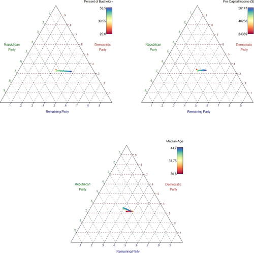
To see the effects of the covariates, we estimated the model (4.1) using the whole dataset with the Dense-CBS scheme. We obtained that ${\widehat{\beta }}_1=2.454$. The result with such a large positive value demonstrates that the party supporting tendency in the 2020 U.S. election is tied strongly with that in the 2016 election. Thus, the empirical result provides a strong evidence that the underlying political orientation is an important determinant for the presidential election. The estimated component maps are depicted in Figure 1, which visualize the effects of the socio-demographic variables on the election results. A clear lesson from the estimated maps is that the approval rate for the Democratic candidate remains unchanged as education level or income level increases, while it decreases for the Republican candidate and increases for the group of other candidates. The effects of age do not seem to have a monotone pattern.

Fig. 1 The estimated component maps ${\widehat{\mathbf{m}}}_k$ for the population characteristics based on the proposed method applied to the U.S. election data.

7 Theoretical Development

7.1 Asymptotic Theory: Scalar Covariates

Here, we discuss the case where ${\mathbf{X}}_i$ and ${\mathbf{Z}}_i$ take values in ${\mathbb{R}}^p$ and ${[0,1]}^d$, respectively. We assume that $({\mathbf{X}}_i,{\mathbf{Z}}_i,{\mathit{\epsilon }}_i)$ for $1\le i\le n$ are iid copies of $(\mathbf{X},\mathbf{Z},\mathit{\epsilon })$ such that $\mathrm{E}(\mathit{\epsilon }|\mathbf{X},\mathbf{Z})=\mathbf{0}$. Recall that $m_{X_j,+}$, for each $1\le j\le p$, is the solution of (2.3) with $\mathbf{W}=X_j$, $m_{\mathbf{X},+}={(m_{X_1,+},\dots ,m_{X_p,+})}^{\top }:{[0,1]}^d\to {\mathbb{R}}^p,{\varrho }_{X_j}=X_j-m_{X_j,+}(\mathbf{Z})$ and ${\varrho }_{\mathbf{X}}={({\varrho }_{X_1},\dots ,{\varrho }_{X_p})}^{\top }$. We let $(h_k:1\le k\le d)$ denote the bandwidth set we use in the construction of ${\widehat{m}}_{\mathbf{X},+}$ and ${\widehat{\mathbf{m}}}_{\mathbf{Y},+}$ for $\widehat{\mathit{\beta }}$ and ${\widehat{\mathit{\beta }}}_0$. Recall ${\widehat{\mathbf{m}}}_{+}={\widehat{\mathbf{m}}}_{\mathbf{Y} \ominus {\widehat{\mathit{\beta }}}_0 \ominus ({\mathbf{X}}^{\top }\odot \widehat{\mathit{\beta }}), +}$, which solves (2.5) with ${\mathbf{W}}_i={\mathbf{Y}}_i \ominus {\widehat{\mathit{\beta }}}_0 \ominus ({\mathbf{X}}_i^{\top }\odot \widehat{\mathit{\beta }})$. We let $(b_k:1\le k\le d)$ denote the bandwidth set we use in the construction of ${\widehat{\mathbf{m}}}_{+}$ with $\widehat{\mathit{\beta }}$ and ${\widehat{\mathit{\beta }}}_0$ at hand.

7.1.1 Technical Assumptions and Invertibility of $n^{-1}{\sum }_{i=1}^n{\tilde{\mathbf{X}}}_i{\tilde{\mathbf{X}}}_i^{\top }$

We collect the technical assumptions we use for our theoretical development.

• (A1) The joint density f is bounded away from zero and infinity on its support ${[0,1]}^d$ and all f_jk are continuously differentiable on ${[0,1]}^2$.

• (A2) The real-valued additive functions $m_{X_j,+}$ are twice continuously differentiable on ${[0,1]}^d$ and the $\mathbb{H}$-valued ${\mathbf{m}}_k$ are twice continously Fréchet differentiable on $[0,1]$.

• (A3) The Hilbertian error variable $\mathit{\epsilon }$ satisfies $\mathrm{E}(|\left|\mathit{\epsilon }\right|{|}^{\alpha })<\infty$ for some $\alpha >12/5$ when $\mathbb{H}$ is finite-dimensional and $\alpha >5/2$ when $\mathbb{H}$ is infinite-dimensional. Also, there exists a constant $0<C_1<\infty$ such that $\mathrm{E}(|\left|\mathit{\epsilon }\right|{|}^2|\mathbf{X},\mathbf{Z})\le C_1$ a.s.

• (A4) The p × p matrix $\mathrm{E}({\varrho }_{\mathbf{X}} {\varrho }_{\mathbf{X}}^{\top })$ is invertible.

• (A5) There exist constants $0<L,C_2<\infty$ such that ${\max }_{1\le j\le p}\mathrm{E}(\hspace{0.17em}\exp \hspace{0.17em}(|X_j|/L)|\mathbf{Z})\le C_2$ a.s.

• (A6) The baseline kernel K is symmetric and positive on $(-1,1)$ but it vanishes on $\mathbb{R}\setminus (-1,1)$ and its first derivative is Lipschitz continuous.

• (A7) The bandwidths h_k satisfy $h_k\asymp n^{-\gamma }$ for some γ with $1/6<\gamma <\min \{1/3,(\alpha -2)/\alpha \}$ when $\mathbb{H}$ is finite-dimensional, and with $1/5<\gamma <\min \{1/3,(\alpha -2)/\alpha \}$ when $\mathbb{H}$ is infinite-dimensional.

• (A8) The bandwidths b_k satisfy that $b_k\to 0$ and $\underset{n}{\lim \inf }{n}^{c_k}{b}_k>0$ for some constants $c_k<(\alpha -2)/\alpha$ for all $1\le k\le d$, and ${(n{b}_j{b}_k)}^{-1}\hspace{0.17em}\log \hspace{0.17em}n\to 0$ for all $1\le j\ne k\le d$.

The conditions (A1) and (A2) for ${\mathbf{m}}_k$ are typically assumed in the smooth backfitting literature, see Jeon and Park (2020). The moment conditions at (A3) ensure $(\alpha -2)/\alpha >1/6$ for finite-dimensional $\mathbb{H}$ and $(\alpha -2)/\alpha >1/5$ for infinite-dimensional $\mathbb{H}$, so that the bandwidth ranges in (A7) make sense. The range for infinite-dimensional $\mathbb{H}$ does not cover the optimal size for univariate nonparametric smoothing, which is $n^{-1/5}$, but we note that the bandwidths h_k are for estimating the parametric part of the model, not for the nonparametric part. For the latter, we use b_k for which we assume (A8). The condition (A4) ensures that the matrix $n^{-1}{\sum }_{i=1}^n{\tilde{\mathbf{X}}}_i{\tilde{\mathbf{X}}}_i^{\top }$ is invertible with probability tending to one, which we detail below. The exponential moment condition (A5) is assumed to use empirical process theory (e.g., van de Geer 2000) in developing technical discussion for ${\widehat{\mathit{\beta }}}_j$. The condition (A6) is stronger than the typical one in kernel smoothing that K itself is Lipschitz continuous. The latter condition is required to make our estimator ${\widehat{\mathbf{m}}}_{+}$ smoother, so that it belongs to an $\mathbb{H}$-valued function class with a proper entropy.

We now state a proposition that demonstrates the invertibility of $n^{-1}{\sum }_{i=1}^n{\tilde{\mathbf{X}}}_i{\tilde{\mathbf{X}}}_i^{\top }$.

Proposition 7.1.

Assume (A1), (A2) for $m_{X_j,+}$ and (A4)–(A7). Then, $$n^{-1}\sum _{i=1}^n{\tilde{\mathbf{X}}}_i{\tilde{\mathbf{X}}}_i^{\top }=\mathrm{E}({\varrho }_{\mathbf{X}} {\varrho }_{\mathbf{X}}^{\top })+O_p(n^{-2\gamma }+n^{-(1-\gamma )/2}\sqrt{\hspace{0.17em}\log \hspace{0.17em}n}),$$so that $n^{-1}{\sum }_{i=1}^n{\tilde{\mathbf{X}}}_i{\tilde{\mathbf{X}}}_i^{\top }$ is invertible with probability tending to one.

7.1.2 Estimation of Parametric Components

We present the limit distribution of $\widehat{\mathit{\beta }}$ defined at (3.7). For this we need to introduce several terminologies. First, we let ${\mathbb{H}}^p$ be equipped with an inner product ${〈·,·〉}_{\text{tp}}$ defined by ${〈\mathbf{a},\mathbf{b}〉}_{\text{tp}}={\sum }_{j=1}^p〈{\mathbf{a}}_j,{\mathbf{b}}_j〉$ for $\mathbf{a}={({\mathbf{a}}_1,\dots ,{\mathbf{a}}_p)}^{\top }$ and $\mathbf{b}={({\mathbf{b}}_1,\dots ,{\mathbf{b}}_p)}^{\top }$ in ${\mathbb{H}}^p$. Let $\left|\right|·|{|}_{\text{tp}}$ be the associated norm such that $\left|\right|\mathbf{a}|{|}_{\text{tp}}^2={\sum }_{j=1}^p|\left|{\mathbf{a}}_j\right|{|}^2$. For $\mathbf{e}\in \mathbb{H}$, define $\mathbf{e}\otimes \mathbf{e}:{\mathbb{H}}^p\to {\mathbb{H}}^p$, an outer product in ${\mathbb{H}}^p$, by $$(\mathbf{e}\otimes \mathbf{e})(\mathbf{a})={\left(〈\mathbf{e},{\mathbf{a}}_1〉\odot \mathbf{e},\dots ,〈\mathbf{e},{\mathbf{a}}_p〉\odot \mathbf{e}\right)}^{\top }.$$

For a general ${\mathbb{H}}^p$-valued random element V, a linear operator $\mathbf{S}:{\mathbb{H}}^p\to {\mathbb{H}}^p$ such that $$\text{cov}({〈\mathbf{V},\mathbf{a}〉}_{\text{tp}},{〈\mathbf{V},\mathbf{b}〉}_{\text{tp}})={〈\mathbf{S}(\mathbf{a}),\mathbf{b}〉}_{\text{tp}},\hspace{1em}\mathbf{a},\mathbf{b}\in {\mathbb{H}}^p$$is called the covariance operator of V. For a random vector U taking values in ${\mathbb{R}}^p$, $$\text{cov}\left({〈\mathbf{U}\odot \mathit{\epsilon },\mathbf{a}〉}_{\text{tp}},{〈\mathbf{U}\odot \mathit{\epsilon },\mathbf{b}〉}_{\text{tp}}\right)={〈\mathrm{E}[\mathbf{U}{\mathbf{U}}^{\top }\odot (\mathit{\epsilon }\otimes \mathit{\epsilon })(\mathbf{a})], \mathbf{b}〉}_{\text{tp}},$$ so that $\mathrm{E}[\mathbf{U}{\mathbf{U}}^{\top }\odot (\mathit{\epsilon }\otimes \mathit{\epsilon })]:{\mathbb{H}}^p\to {\mathbb{H}}^p$, defined by $\mathrm{E}[\mathbf{U}{\mathbf{U}}^{\top }\odot (\mathit{\epsilon }\otimes \mathit{\epsilon })](\mathbf{a})=\mathrm{E}[\mathbf{U}{\mathbf{U}}^{\top }\odot (\mathit{\epsilon }\otimes \mathit{\epsilon })(\mathbf{a})]$, is the covariance operator of $\mathbf{U}\odot \mathit{\epsilon }$. Let $\mathbf{G}({\mathbf{0}}_p,\mathbf{S})$ denote a Gaussian random element taking values in ${\mathbb{H}}^p$ with mean ${\mathbf{0}}_p={(\mathbf{0},\dots ,\mathbf{0})}^{\top }\in {\mathbb{H}}^p$ and covariance operator S, that is, the real-valued random variable ${〈\mathbf{G}({\mathbf{0}}_p,\mathbf{S}),\mathbf{a}〉}_{\text{tp}}$ for any $\mathbf{a}\in {\mathbb{H}}^p$ is normally distributed with mean 0 and variance ${〈\mathbf{S}(\mathbf{a}),\mathbf{a}〉}_{\text{tp}}$. Let $\mathbf{\Sigma }=\mathrm{E}[{(\mathrm{E} {\varrho }_{\mathbf{X}} {\varrho }_{\mathbf{X}}^{\top })}^{-1}·{\varrho }_{\mathbf{X}}{\varrho }_{\mathbf{X}}^{\top }·{(\mathrm{E} {\varrho }_{\mathbf{X}} {\varrho }_{\mathbf{X}}^{\top })}^{-1}\odot (\mathit{\epsilon }\otimes \mathit{\epsilon })]$, which is the covariance operator of ${(\mathrm{E} {\varrho }_{\mathbf{X}}{\varrho }_{\mathbf{X}}^{\top })}^{-1}{\varrho }_{\mathbf{X}}\odot \mathit{\epsilon }$. Note that, in case $\mathit{\epsilon }$ is independent of $(\mathbf{X},\mathbf{Z})$, then $\mathbf{\Sigma }$ reduces to ${(\mathrm{E} {\varrho }_{\mathbf{X}} {\varrho }_{\mathbf{X}}^{\top })}^{-1}$ $\odot \mathrm{E}(\mathit{\epsilon }\otimes \mathit{\epsilon })$.

Theorem 7.1.

Under the assumptions (A1)–(A7), it holds that $$\begin{array}{cc}\sqrt{n}\odot (\widehat{\mathit{\beta }} \ominus \mathit{\beta })\hfill & =n^{-1/2}\odot ({\oplus }_{i=1}^n{(\mathrm{E} {\varrho }_{\mathbf{X}}{\varrho }_{\mathbf{X}}^{\top })}^{-1}{\varrho }_{\mathbf{X},i}\odot {\mathit{\epsilon }}_i)\hfill \\ \hfill & \hspace{1em}+o_p(1)\hfill \\ \hfill & \hspace{1em}⇝ \mathbf{G}({\mathbf{0}}_p,\mathbf{\Sigma }).\hfill \end{array}$$

The following corollary for ${\widehat{\mathit{\beta }}}_0=\overline{\mathbf{Y}} \ominus ({\oplus }_{j=1}^p{\overline{X}}_j\odot {\widehat{\mathit{\beta }}}_j)$ is an immediate consequence of Theorem 7.1. Recall that ${\mathit{\beta }}_0=\mathrm{E}(\mathbf{Y}) \ominus ({\oplus }_{j=1}^p\mathrm{E}(X_j)\odot {\mathit{\beta }}_j)$.

Corollary 7.1.

Under the assumptions (A1)–(A7), it holds that $\left|\right|{\widehat{\mathit{\beta }}}_0 \ominus {\mathit{\beta }}_0\left|\right|=O_p(n^{-1/2})$.

7.1.3 Comparison with HPLM

We make a theoretical comparison of $\widehat{\mathit{\beta }}$ and ${\widehat{\mathit{\beta }}}^{\text{PLM}}$, the latter of which is defined at (3.11). Let ${\mathbf{\Sigma }}^{\text{PLM}}=\mathrm{E}[{(\mathrm{E} {ϵ}_{\mathbf{X}} {ϵ}_{\mathbf{X}}^{\top })}^{-1}·{ϵ}_{\mathbf{X}}{ϵ}_{\mathbf{X}}^{\top }·{(\mathrm{E} {ϵ}_{\mathbf{X}} {ϵ}_{\mathbf{X}}^{\top })}^{-1}\odot (\mathit{\epsilon }\otimes \mathit{\epsilon })]$. Then, along the lines of the proof of Theorem 7.1 in the supplement S.11, we may prove that, under suitable conditions, (7.1) $$\begin{array}{c}\sqrt{n}\odot ({\widehat{\mathit{\beta }}}^{\text{PLM}} \ominus \mathit{\beta }) ⇝ \mathbf{G}({\mathbf{0}}_p,{\mathbf{\Sigma }}^{\text{PLM}}).\hfill \end{array}$$(7.1)

A special case of (7.1) for $\mathbb{H}=\mathbb{R}$ and d = 1 has been derived by Liang (2006). The result (7.1) for ${\widehat{\mathit{\beta }}}^{\text{PLM}}$ is valid under the PLM and thus remains true under the PLAM as well. In case $\mathit{\epsilon }$ is independent of $(\mathbf{X},\mathbf{Z}),{\mathbf{\Sigma }}^{\text{PLM}}$ reduces to ${(\mathrm{E} {ϵ}_{\mathbf{X}} {ϵ}_{\mathbf{X}}^{\top })}^{-1}\odot \mathrm{E}(\mathit{\epsilon }\otimes \mathit{\epsilon })$. The following definition is an extension of the classical notion of “asymptotic efficiency” for real-valued parameters to that for Hilbertian parameters.

Definition 7.1.

Let ${\widehat{\mathit{\theta }}}_1$ and ${\widehat{\mathit{\theta }}}_2$ be estimators of a parameter $\mathit{\theta }$ in a separable Hilbert space $\mathcal{H}$ such that $s_n\odot ({\widehat{\mathit{\theta }}}_j \ominus \mathit{\theta })⇝\mathbf{G}(\mathbf{0},{\mathbf{\Sigma }}_j)$ for a sequence s_n and covariance operators ${\mathbf{\Sigma }}_j$ for j = 1, 2. We say that ${\widehat{\mathit{\theta }}}_1$ is asymptotically more efficient than ${\widehat{\mathit{\theta }}}_2$ if ${\mathbf{\Sigma }}_1-{\mathbf{\Sigma }}_2$ is a nonnegative definite operator, that is, $〈({\mathbf{\Sigma }}_1-{\mathbf{\Sigma }}_2)(\mathbf{h}),\mathbf{h}〉\ge 0$ for all $\mathbf{h}\in \mathcal{H}$.

We note that ${(\mathrm{E} {ϵ}_{\mathbf{X}} {ϵ}_{\mathbf{X}}^{\top })}^{-1}-{(\mathrm{E} {\varrho }_{\mathbf{X}} {\varrho }_{\mathbf{X}}^{\top })}^{-1}$ is nonnegative definite and it is zero only if $m_{\mathbf{X}}=m_{\mathbf{X},+}$. A direct computation shows that (7.2) $$\begin{array}{cc}\hfill & {〈({\mathbf{\Sigma }}^{\text{PLM}}-\mathbf{\Sigma })(\mathbf{a}),\mathbf{a}〉}_{\text{tp}}\hfill \\ \hfill & =\mathrm{E}[(〈\mathit{\epsilon },{\mathbf{a}}_1〉,\dots ,〈\mathit{\epsilon },{\mathbf{a}}_p〉)·({(\mathrm{E} {ϵ}_{\mathbf{X}}{ϵ}_{\mathbf{X}}^{\top })}^{-1}-{(\mathrm{E} {\varrho }_{\mathbf{X}}{\varrho }_{\mathbf{X}}^{\top })}^{-1})\hfill \\ \hfill & \hspace{1em}·{(〈\mathit{\epsilon },{\mathbf{a}}_1〉,\dots ,〈\mathit{\epsilon },{\mathbf{a}}_p〉)}^{\top }],\hfill \end{array}$$(7.2) which implies that $\widehat{\mathit{\beta }}$ is asymptotically more efficient than ${\widehat{\mathit{\beta }}}^{\text{PLM}}$ in the sense of Definition 7.1. Let d_j denote the jth diagonal entry of ${(\mathrm{E} {ϵ}_{\mathbf{X}} {ϵ}_{\mathbf{X}}^{\top })}^{-1}-{(\mathrm{E} {\varrho }_{\mathbf{X}} {\varrho }_{\mathbf{X}}^{\top })}^{-1}$. Then, under the PLAM (3.1), it holds that $$n·\left(\left|\right|{\widehat{\mathit{\beta }}}_j^{\text{PLM}} \ominus {\mathit{\beta }}_j|{|}^2-||{\widehat{\mathit{\beta }}}_j \ominus {\mathit{\beta }}_j|{|}^2\right)=S_{nj}+o_p(1)$$ with $\mathrm{E}(S_{nj})=d_j·\mathrm{E}(|\left|\mathit{\epsilon }\right|{|}^2)$, which is the gain by ${\widehat{\mathit{\beta }}}_j$ against ${\widehat{\mathit{\beta }}}_j^{\text{PLM}}$ under (3.1).

7.1.4 Estimation of Nonparametric Components

As we discussed in Section 3.3, ${\widehat{\mathbf{m}}}_{+}$ is uniquely decomposed into ${\widehat{\mathbf{m}}}_{+}={\oplus }_{j=1}^d{\widehat{\mathbf{m}}}_j$ with the constraints at (3.8). We study the error rates for ${\widehat{\mathbf{m}}}_{+}$ and ${\widehat{\mathbf{m}}}_k$. The asymptotic results presented here do not follow immediately from the results in Jeon and Park (2020) since ${\mathbf{Y}}_i \ominus {\widehat{\mathit{\beta }}}_0 \ominus ({\mathbf{X}}_i^{\top }\odot \widehat{\mathit{\beta }})\ne {\mathbf{m}}_{+}({\mathbf{Z}}_i) \oplus \mathit{\epsilon }$. Furthermore, as seen in the assumption (A8), our work allows for a flexible range for the bandwidths b_k, instead of assuming $b_k\asymp n^{-1/5}$ as in Jeon and Park (2020). Put ${\kappa }_k(\tau )=b_k^{\tau }+{(n{b}_k)}^{-1/2}\sqrt{\hspace{0.17em}\log \hspace{0.17em}n}$ for $\tau =1,2$ and $1\le k\le d$. Also, let ${\delta }_k={\max }_{\mathcal{l}\ne k}{b}_{\mathcal{l}}^2+n^{-1/2}·{({\min }_{\mathcal{l}\ne k}{b}_{\mathcal{l}})}^{-1/2}$.

Theorem 7.2.

Assume (A1)–(A8). Then, it holds that, for each $1\le k\le d$, $$\begin{array}{cc}\underset{z_k\in [2b_k,1-2b_k]}{\sup }\left|\right|{\widehat{\mathbf{m}}}_k(z_k) \ominus {\mathbf{m}}_k(z_k)\left|\right|\hfill & =O_p({\kappa }_k(2)+{\delta }_k),\hfill \\ \underset{z_k\in [0,1]}{\sup }\left|\right|{\widehat{\mathbf{m}}}_k(z_k) \ominus {\mathbf{m}}_k(z_k)\left|\right|\hfill & =O_p({\kappa }_k(1)+{\delta }_k).\hfill \end{array}$$

Consequently, $$\begin{array}{cc}\underset{\mathbf{z}\in [2b_1,1-2b_1]\times \cdots \times [2b_d,1-2b_d]}{\sup }\left|\right|{\widehat{\mathbf{m}}}_{+}(\mathbf{z}) \ominus {\mathbf{m}}_{+}(\mathbf{z})\left|\right|\hfill & =O_p(\underset{1\le k\le d}{\max }{\kappa }_k(2)),\hfill \\ \underset{\mathbf{z}\in {[0,1]}^d}{\sup }\left|\right|{\widehat{\mathbf{m}}}_{+}(\mathbf{z}) \ominus {\mathbf{m}}_{+}(\mathbf{z})\left|\right|\hfill & =O_p(\underset{1\le k\le d}{\max }{\kappa }_k(1)).\hfill \end{array}$$

In the case where $b_k\asymp n^{-1/5}$ for all $1\le k\le d$, the rates in Theorem 7.2 reduce to the usual ones for univariate smoothing. Indeed, for each $1\le k\le d$, $$\begin{array}{cc}\underset{z_k\in [2b_k,1-2b_k]}{\sup }\left|\right|{\widehat{\mathbf{m}}}_k(z_k) \ominus {\mathbf{m}}_k(z_k)\left|\right|\hfill & =O_p\left(n^{-2/5}\sqrt{\hspace{0.17em}\log \hspace{0.17em}n}\right),\hfill \\ \underset{z_k\in [0,1]}{\sup }\left|\right|{\widehat{\mathbf{m}}}_k(z_k) \ominus {\mathbf{m}}_k(z_k)\left|\right|\hfill & =O_p(n^{-1/5}).\hfill \end{array}$$

We also derive the asymptotic distributions of ${\widehat{\mathbf{m}}}_{+}$ and ${\widehat{\mathbf{m}}}_k$, which we defer to the supplement S.15.

7.2 Asymptotic Theory: Hilbertian Covariates

Here, we discuss the case where the covariates in the linear part of the model, which we denoted by ${\mathbf{X}}_j$ for $1\le j\le p$, take values in $\mathbb{H}$. Define now ${\mathit{\varrho }}_{{\mathbf{X}}_j}={\mathbf{X}}_j \ominus {\mathbf{m}}_{{\mathbf{X}}_j,+}(\mathbf{Z})$. Recall that $\mathrm{E}(〈〈{\mathit{\varrho }}_{\mathbf{X}},{\mathit{\varrho }}_{\mathbf{X}}〉〉)$ is the p × p matrix whose (j, k) element equals $\mathrm{E}(〈{\mathit{\varrho }}_{{\mathbf{X}}_j},{\mathit{\varrho }}_{{\mathbf{X}}_k}〉)$. We first introduce some technical assumptions for Hilbertian ${\mathbf{X}}_j$. We note that the assumptions (A1), (A6) and (A8) in Section 7.1 still apply in the present case, which we call (B1), (B6), and (B8), respectively, here. The corresponding versions of the others are given below.

• (B2) The $\mathbb{H}$-valued ${\mathbf{m}}_{{\mathbf{X}}_j,+}$ are twice continuously Fréchet differentiable on ${[0,1]}^d$ and the $\mathbb{H}$-valued ${\mathbf{m}}_k$ at (4.1) are twice continously Fréchet differentiable on $[0,1]$.

• (B3) The Hilbertian error variable $\mathit{\epsilon }$ at (4.1) satisfies $\mathrm{E}(|\left|\mathit{\epsilon }\right|{|}^{\alpha })<\infty$ for some $\alpha >12/5$. Also, there exists a constant $0<C_1<\infty$ such that $\mathrm{E}(|\left|\mathit{\epsilon }\right|{|}^2|\mathbf{X},\mathbf{Z})\le C_1$ a.s.

• (B4) The p × p matrix $\mathrm{E}(〈〈{\mathit{\varrho }}_{\mathbf{X}},{\mathit{\varrho }}_{\mathbf{X}}〉〉)$ is invertible.

• (B5) There exist constants $0<L,C_2<\infty$ such that ${\max }_{1\le j\le p}\mathrm{E}(\hspace{0.17em}\exp \hspace{0.17em}(|\left|{\mathbf{X}}_j\right||/L)|\mathbf{Z})\le C_2$ a.s.

• (B7) The bandwidths h_k satisfy $h_k\asymp n^{-\gamma }$ for some γ with $1/6<\gamma <\min \{1/3,(\alpha -2)/\alpha \}$.

The conditions (B3) and (B7) are the same as (A3) and (A7), respectively, for finite-dimensional $\mathbb{H}$. In fact, for infinite-dimensional $\mathbb{H}$, we are able to derive a slower rate for $\widehat{\mathit{\beta }}$ and ${\widehat{\mathit{\beta }}}_0$, see below the second parts of Theorem 7.3 and Corollary 7.2. For such rate of convergence, we find that (B3) and (B7) are sufficient. The following proposition is an analogue of Proposition 7.1 for Hilbertian ${\mathbf{X}}_j$.

Proposition 7.2.

Assume (B1), (B2) for ${\mathbf{m}}_{{\mathbf{X}}_j,+}$ and (B4)–(B7). Then, $$n^{-1}\sum _{i=1}^n〈〈{\tilde{\mathbf{X}}}_i,{\tilde{\mathbf{X}}}_i〉〉\mathrm{}=\mathrm{}\mathrm{E}(〈〈{\mathit{\varrho }}_{\mathbf{X}},{\mathit{\varrho }}_{\mathbf{X}}〉〉)\mathrm{}+\mathrm{}{O}_p(n^{-2\gamma }\mathrm{}+\mathrm{}{n}^{-(1-\gamma )/2}\sqrt{\hspace{0.17em}\log \hspace{0.17em}n}),$$ so that $n^{-1}{\sum }_{i=1}^n〈〈{\tilde{\mathbf{X}}}_i,{\tilde{\mathbf{X}}}_i〉〉$ is invertible with probability tending to one.

We now derive the asymptotic properties of $\widehat{\mathit{\beta }}$. Note that $\mathrm{E}(〈〈{\mathit{\varrho }}_{\mathbf{X}},\mathit{\epsilon }〉〈\mathit{\epsilon },{\mathit{\varrho }}_{\mathbf{X}}〉〉)$ is the p × p matrix whose (j, k) element is given by $\mathrm{E}(〈{\mathit{\varrho }}_{{\mathbf{X}}_j},\mathit{\epsilon }〉〈{\mathit{\varrho }}_{{\mathbf{X}}_k},\mathit{\epsilon }〉)$. Define $${\Sigma }_p={(\mathrm{E}(〈〈{\mathit{\varrho }}_{\mathbf{X}},{\mathit{\varrho }}_{\mathbf{X}}〉〉))}^{-1}·\mathrm{E}(〈〈{\mathit{\varrho }}_{\mathbf{X}},\mathit{\epsilon }〉〈\mathit{\epsilon },{\mathit{\varrho }}_{\mathbf{X}}〉〉)·{(\mathrm{E}(〈〈{\mathit{\varrho }}_{\mathbf{X}},{\mathit{\varrho }}_{\mathbf{X}}〉〉))}^{-1}.$$

Let $N_p(0_p,{\Sigma }_p)$ denote the multivariate normal distribution with mean $0_p={(0,\dots ,0)}^{\top }\in {\mathbb{R}}^p$ and covariance matrix Σ_p.

Theorem 7.3.

Assume (B1)–(B7). If $\mathbb{H}$ is finite-dimensional, then it holds that $$\begin{array}{cc}\sqrt{n}(\widehat{\mathit{\beta }}-\mathit{\beta })\hfill & =n^{-1/2}·\sum _{i=1}^n(\mathrm{E} 〈〈{\mathit{\varrho }}_{\mathbf{X}},{\mathit{\varrho }}_{\mathbf{X}}〉〉{)}^{-1}〈〈{\mathit{\varrho }}_{\mathbf{X},i},{\mathit{\epsilon }}_i〉+o_p(1)\hfill \\ \hfill & \hspace{1em}⇝ N_p(0_p,{\Sigma }_p).\hfill \end{array}$$

If $\mathbb{H}$ is infinite-dimensional, then $\widehat{\mathit{\beta }}-\mathit{\beta }=O_p(n^{-2\gamma }\hspace{0.17em}\log \hspace{0.17em}n+n^{-(1-\gamma )/2}{(\hspace{0.17em}\log \hspace{0.17em}n)}^{3/2})$.

The following corollary for ${\widehat{\mathit{\beta }}}_0=\overline{\mathbf{Y}} \ominus {\oplus }_{j=1}^p{\widehat{\beta }}_j\odot {\overline{\mathbf{X}}}_j$ is an immediate consequence of Theorem 7.3. Recall that ${\mathit{\beta }}_0=\mathrm{E}(\mathbf{Y}) \ominus {\oplus }_{j=1}^p{\beta }_j\odot \mathrm{E}({\mathbf{X}}_j)$.

Corollary 7.2.

Assume (B1)–(B7). If $\mathbb{H}$ is finite-dimensional, then $\left|\right|{\widehat{\mathit{\beta }}}_0 \ominus {\mathit{\beta }}_0\left|\right|=O_p(n^{-1/2})$. If $\mathbb{H}$ is infinite-dimensional, then $\left|\right|{\widehat{\mathit{\beta }}}_0 \ominus {\mathit{\beta }}_0\left|\right|=O_p(n^{-2\gamma }\hspace{0.17em}\log \hspace{0.17em}n+n^{-(1-\gamma )/2}{(\hspace{0.17em}\log \hspace{0.17em}n)}^{3/2})$.

Next, we present the asymptotic properties of ${\widehat{\mathbf{m}}}_{+}$ and ${\widehat{\mathbf{m}}}_k$ satisfying the constraints at (3.8). As in Section 7.1, we let $(b_k:1\le k\le d)$ denote the set of bandwidths for defining (2.5) with ${\mathbf{W}}_i={\mathbf{Y}}_i \ominus {\widehat{\mathit{\beta }}}_0 \ominus {\oplus }_{j=1}^p({\widehat{\beta }}_j\odot {\mathbf{X}}_{ij})$. Recall ${\kappa }_k(\tau )=b_k^{\tau }+{(n{b}_k)}^{-1/2}\sqrt{\hspace{0.17em}\log \hspace{0.17em}n}$ and ${\delta }_k={\max }_{\mathcal{l}\ne k}{b}_{\mathcal{l}}^2+n^{-1/2}·{({\min }_{\mathcal{l}\ne k}{b}_{\mathcal{l}})}^{-1/2}$. Put ${\tilde{\delta }}_k={\delta }_k$ if $\mathbb{H}$ is finite-dimensional, and ${\tilde{\delta }}_k={\delta }_k+n^{-2\gamma }{(\hspace{0.17em}\log \hspace{0.17em}n)}^2+n^{-(1-\gamma )/2}{(\hspace{0.17em}\log \hspace{0.17em}n)}^{5/2}$ if $\mathbb{H}$ is infinite-dimensional.

Theorem 7.4.

Assume (B1)–(B8). Then, Theorem 7.2 remains to hold with δ_k being replaced by ${\tilde{\delta }}_k$.

We also derive the asymptotic distributions of ${\widehat{\mathbf{m}}}_{+}$ and ${\widehat{\mathbf{m}}}_k$ in the case of Hilbertian ${\mathbf{X}}_j$, which we defer to the supplement S.18.

Supplementary Materials

The supplementary material contains the description of the CBS algorithm, the geometries of Bayes-Hilbert spaces and simplices, and an additional real data application. It also includes two additional theorems for the asymptotic distributions of the estimators of the nonparametric components of the partially linear additive models, and all technical proofs.

Acknowledgments

The authors thank an Associate Editor and two referees for giving thoughtful and constructive comments on the earlier versions of the article.

Additional information

Funding

Byeong U. Park’s research was supported by the National Research Foundation of Korea (NRF) grant funded by the Korea government (MSIP) (No. 2019R1A2C3007355). Kyusang Yu’s research was supported by the National Research Foundation of Korea (NRF) funded by the Korea government (MSIT) NRF-2021R1A4A5032622.

References

- Benatia, D., Carrasco, M., and Florens, J.-P. (2017), “Functional Linear Regression with Functional Response,” Journal of Econometrics, 201, 269–291. DOI: 10.1016/j.jeconom.2017.08.008.
- Bhattacharya, P. K., and Zhao, P.-L. (1997), “Semiparametric Inference in a Partial Linear Model,” The Annals of Statistics, 25, 244–262. DOI: 10.1214/aos/1034276628.
- Bissantz, N., Dette, H., Hildebrandt, T., and Bissantz, K. (2016), “Smooth Backfitting in Additive Inverse Regression,” Annals of the Institute of Statistical Mathematics, 68, 827–853. DOI: 10.1007/s10463-015-0517-x.
- Bosq, D. (2000), Linear Processes in Function Spaces, New York: Springer.
- Buja, A., Hastie, T., and Tibshirani, R. (1989), “Linear Smoothers and Additive Models,” (with discussion), The Annals of Statistics, 17, 453–555. DOI: 10.1214/aos/1176347115.
- Hall, P., and Horowitz, J. L. (2007), “Methodology and Convergence Rates for Functional Linear Regression,” The Annals of Statistics, 35, 70–91. DOI: 10.1214/009053606000000957.
- Han, K., and Park, B. U. (2018), “Smooth Backfitting for Errors-in-Variables Additive Models,” The Annals of Statistics, 46, 2216–2250. DOI: 10.1214/17-AOS1617.
- Han, K., Müller, H.-G., and Park, B. U. (2020), “Additive Functional Regression for Densities as Responses,” Journal of the American Statistical Association, 115, 997–1010. DOI: 10.1080/01621459.2019.1604365.
- Horváth, L., and Kokoszka, P. (2012), Inference for Functional Data with Applications, New York: Springer.
- Jeon, J. M., and Park, B. U. (2020), “Additive Regression with Hilbertian Responses,” The Annals of Statistics, 48, 2671–2697. DOI: 10.1214/19-AOS1902.
- Jeon, J. M., Park, B. U., and Van Keilegom, I. (2021), “Additive Regression with Non-Euclidean Responses and Predictors,” The Annals of Statistics, 49, 2611–2641. DOI: 10.1214/21-AOS2048.
- Jeon, J. M., and Van Bever, G. (2022), “Additive Regression with General Imperfect Variables,” arXiv:2212.05745.
- Lee, E. R., Han, K., and Park, B. U. (2018), “Estimation of Errors-in-Variables Partially Linear Additive Models,” Statistica Sinica, 28, 2353–2373.
- Lee, Y. K., Mammen, E., and Park, B. U. (2010), “Backfitting and Smooth Backfitting for Additive Quantile Models,” The Annals of Statistics, 38, 2857–2883. DOI: 10.1214/10-AOS808.
- Lee, Y. K., Mammen, E., and Park, B. U. (2012), “Flexible Generalized Varying Coefficient Regression Models,” The Annals of Statistics, 40, 1906–1933.
- Liang, H. (2006), “Estimation in Partially Linear Models and Numerical Comparisons,” Computational Statistics & Data Analysis, 50, 675–687. DOI: 10.1016/j.csda.2004.10.007.
- Liang, H., Thurston, S. W., Ruppert, D., Apanasovich, T., and Hauser, R. (2008), “Additive Partially Linear Models with Measurement Errors,” Biometrika, 95, 667–678. DOI: 10.1093/biomet/asn024.
- Lin, Z., Müller, H.-G., and Park, B. U. (2022), “Additive Models for Symmetric Positive-Definite Matrices and Lie Groups,” Biometrika (to appear). DOI: 10.1093/biomet/asac055.
- Linton, O., Sperlich, S., and van Keilegom, I. (2008), “Estimation of a Semiparametric Transformation Model,” The Annals of Statistics, 36, 686–718. DOI: 10.1214/009053607000000848.
- Mammen, E., Linton, O., and Nielsen, J. P. (1999), “The Existence and Asymptotic Properties of a Backfitting Projection Algorithm under Weak Conditions,” The Annals of Statistics, 27, 1443–1490. DOI: 10.1214/aos/1017939138.
- Opsomer, J. D., and Ruppert, D. (1997), “Fitting a Bivariate Additive Model by Local Polynomial Regression,” The Annals of Statistics, 25, 186–211. DOI: 10.1214/aos/1034276626.
- Opsomer, J. D., and Ruppert, D. (1999), “A Root-n Consistent Backfitting Estimator for Semiparametric Additive Modeling,” Journal of Computational and Graphical Statistics, 8, 715–732.
- Ramsay, J. O., and Silverman, B. W. (2005), Functional Data Analysis, New York: Springer.
- Severini, T., and Wong, W. (1992), “Profile Likelihood and Conditionally Parametric Models,” The Annals of Statistics, 20, 1768–1802. DOI: 10.1214/aos/1176348889.
- van de Geer, S. (2000), Empirical Processes in M-Estimation, Cambridge: Cambridge University Press.
- Yao, F., Müller, H.-G., and Wang, J.-L. (2005), “Functional Linear Regression Analysis for Longitudinal Data,” The Annals of Statistics, 33, 2873–2903. DOI: 10.1214/009053605000000660.
- Yu, K., Mammen, E., and Park, B. U. (2011), “Semi-Parametric Regression: Efficiency Gains from Modeling the Nonparametric Part,” Bernoulli, 17, 736–748. DOI: 10.3150/10-BEJ296.
- Yu, K., Park, B. U., and Mammen, E. (2008), “Smooth Backfitting in Generalized Additive Models,” The Annals of Statistics, 36, 228–260. DOI: 10.1214/009053607000000596.
- Zhang, X., Park, B. U., and Wang, J.-L. (2013), “Time-Varying Additive Models for Longitudinal Data,” Journal of the American Statistical Association, 108, 983–998. DOI: 10.1080/01621459.2013.778776.