Higher-Order Least Squares: Assessing Partial Goodness of Fit of Linear Causal Models

Abstract

We introduce a simple diagnostic test for assessing the overall or partial goodness of fit of a linear causal model with errors being independent of the covariates. In particular, we consider situations where hidden confounding is potentially present. We develop a method and discuss its capability to distinguish between covariates that are confounded with the response by latent variables and those that are not. Thus, we provide a test and methodology for partial goodness of fit. The test is based on comparing a novel higher-order least squares principle with ordinary least squares. In spite of its simplicity, the proposed method is extremely general and is also proven to be valid for high-dimensional settings. Supplementary materials for this article are available online.

Keywords:

• Causal inference
• Latent confounding
• Model misspecification
• Nodewise regression
• Structural equation models

1 Introduction

Linear models are the most commonly used statistical tools to study the relationship between a response and a set of covariates. The regression coefficient corresponding to a particular covariate is usually interpreted as its net effect on the response variable when all else is held fixed. Such an interpretation is essential in many applications and yet could be rather misleading when the linear model assumptions are in question, in particular, when there are hidden confounders.

In this work, we develop a simple but powerful approach to goodness of fit tests for potentially high-dimensional linear causal models, including also tests for partial goodness of fit of single predictor variables. While hidden confounding is the primary alternative in mind, different nonlinear deviations from the linear model assumption are also in scope. Tests for goodness of fit are essential to statistical modeling (e.g., Lehmann, Romano, and Casella 2005) and the concept is also very popular in econometrics where it is referred to as specification tests. For an overview of such methods; see, for example, Godfrey (1991) or Maddala and Lahiri (2009).

Another set of related works is Buja et al. (2019a, 2019b), which elaborately discusses deviations from the (linear) model and how distributional robustness, that is, robustenss against shifts in the covariates’ distribution, links to correctly specified models. For this, they introduce the definition of “well-specified” statistical functionals. Distributional robustness, implied by well-specification, is also related to the causal interpretation of a linear model as discussed in Peters, Bühlmann, and Meinshausen (2016).

We consider here the question when and which causal effects can be inferred from the ordinary least squares estimator or a debiased Lasso procedure for the high-dimensional setting, even when there is hidden confounding. We address this by partial goodness of fit testing: if the data speaks against a linear causal model, we are able to specify which components of the least squares estimator should be rejected to be linear causal effects and which not. In the case of a joint Gaussian distribution, one cannot detect anything: this corresponds to a well-known unidentifiability result in causality (Hyvärinen and Oja 2000; Peters et al. 2014). But, in certain models, we are able to identify some causal relations. Of particular importance are non-Gaussian linear structural equation models, as used in Shimizu et al. (2006) or Wang and Drton (2020) among others. The latter constructs the causal graph from observational data in a stepwise procedure using a test statistic similar to the one we suggest.

Our strategy has a very different focus than other approaches which do not rely on the least squares principle any longer to deal with the issue of hidden confounding. Most prominent, particularly in econometrics, is the framework of instrumental variables regression: assuming valid instruments, one can identify all causal effects, see, for example, Angrist, Imbens, and Rubin (1996) or the books by Bowden and Turkington (1990) and Imbens and Rubin (2015). The popular Durbin-Wu-Hausman test (Hausman 1978) for validity of instruments bears a relation to our methodology, namely that we are also looking at the difference of two estimators to test goodness of fit.

Our automated partial goodness of fit methodology is easy to be used as it is based on ordinary (or high-dimensional adaptions of) least squares and its novel higher-order version: we believe that this simplicity is attractive for statistical practice.

1.1 Our Contribution

We propose a novel method with a corresponding test, called higher-order least squares (HOLS). The test statistic is based on the residuals from an ordinary least squares or Lasso fit. In that regard, it is related to Shah and Bühlmann (2018) who use “residual prediction” to test for deviation from the linear model. However, our approach does neither assume Gaussian errors nor does it rely on sample splitting, and our novel test statistic has a $\sqrt{n}$ convergence rate (with n denoting the sample size).

In addition to presenting a “global” goodness of fit test for the entire model, we also develop a local interpretation that allows detecting which among the covariates are giving evidence for hidden confounding or nonlinear relations. Thus, we strongly increase the amount of extracted information compared to a global goodness-of-fit test. In particular, in the case of localized (partial) confounding in linear structural equation models, we are able to recover the unconfounded regression parameters for a subset of predictors. This is a setting where techniques assuming dense (essentially global) confounding, as in Ćevid, Bühlmann, and Meinshausen (2020) or Guo, Ćevid, and Bühlmann (2022), fail.

The work by Buja et al. (2019a, 2019b) especially the second paper, shows how to detect deviations in a linear model using reweighting of the data. Our HOLS technique can be seen as a special way of reweighting. In contrast to their work, we provide a simple test statistic that tests for well-specification without requiring any resampling. Furthermore, we provide guarantees for a local interpretation under suitable modeling assumptions while as their per-covariate view remains rather exploratory.

1.2 Outline

The remainder of this article will be structured as follows. We conclude this section with the necessary notation. In Section 2, we present the main idea of HOLS and the according global null hypothesis. For illustrative purposes, we first discuss univariate regression. Then, we consider multivariate regression and extend our theory to high-dimensional problems incorporating the (debiased) Lasso. In Section 3, we present the local interpretation when the global null does not hold true alongside with theoretical guarantees. Models for which this local interpretation is most suitable are discussed in Section 4. Section 5 contains a real data analysis. We conclude with a summarizing discussion in Section 6.

1.3 Notation

We present some notation that is used throughout this work. Vectors and matrices are written in boldface, while scalars have the usual lettering. This holds for both random and fixed quantities. We use upper case letters to denote a random variable, for example, X or Y. We use lower case letters to denote iid copies of a random variable, for example, x. If $\mathbf{X}\in {\mathbb{R}}^p$, then $\mathbf{x}\in {\mathbb{R}}^{n\times p}$. With a slight abuse of notation, x can either denote the copies or realizations thereof. We write ${\mathbf{x}}_j$ to denote the jth column of matrix x and ${\mathbf{x}}_{-j}$ to denote all but the jth column. We write $\stackrel{H_0}{=}$ to state that equality holds under H₀. With ←, we emphasize that an equality between random variables is induced by a causal mechanism. We use $\odot$ to denote elementwise multiplication of two vectors, for example, $\mathbf{x}\odot \mathbf{y}$. Similarly, potencies of vectors are also to be understood in an elementwise fashion, for example, ${\mathbf{x}}^2=\mathbf{x}\odot \mathbf{x}$. ${\mathit{I}}_n$ is the n-dimensional identity matrix. ${\mathit{P}}_{-j}$ denotes the orthogonal projection onto ${\mathbf{x}}_{-j}$ and ${\mathit{P}}_{-j}^{\perp }={\mathit{I}}_n-{\mathit{P}}_{-j}$ denotes the orthogonal projection onto its complement. For some random vector X, we have the moment matrix ${\mathbf{\Sigma }}^{\mathbf{X}}:=\mathbb{E}\left[\mathbf{X}{\mathbf{X}}^{\top }\right]$. Note that this equals the covariance matrix for centered X. We denote statistical independence by $\perp$. We write e to denote a vector for which every entry is 1 and ${\mathbf{e}}_j$ to denote the unit vector in the direction of the jth coordinate axis.

2 Higher-Order Least Squares (HOLS)

We develop here the main idea of HOLS estimation.

2.1 Univariate Regression as a Motivating Case

It is instructive to begin with the case of simple linear regression where we have a pair of random variables X and Y. We consider the causal linear model (1) $$\begin{array}{c}Y\leftarrow X\beta +\mathcal{E},\hspace{1em}\text{where}\hspace{1em}X\perp \mathcal{E},\\ \hspace{1em}\hspace{1em}\hspace{1em}\mathbb{E}\left[\mathcal{E}\right]=0\hspace{1em}\text{and}\hspace{1em}\mathbb{E}\left[{\mathcal{E}}^2\right]={\sigma }^2<\infty .\end{array}$$(1)

We formulate a null hypothesis that the model in (1) is correct and we denote such a hypothesis by H₀. This model is of interest as β describes the effect of a unit change if we were to intervene on covariate X without intervening on the independent $\mathcal{E}$. Such model, or its multivariate extension, is often assumed in causal discovery, see, for example, Shimizu et al. (2006) or Hoyer et al. (2008). Therefore, we aim to provide a test for its well-specification.

Estimation of the regression parameter is typically done by the least squares principle$${\beta }^{\text{OLS}}:=\underset{b\in \mathbb{R}}{\text{argmin}}\mathbb{E}\left[{\left(Y-Xb\right)}^2\right]=\frac{\mathbb{E}\left[XY\right]}{\mathbb{E}\left[X^2\right]}\stackrel{H_0}{=}\beta ,$$where we use the superscript OLS to denote ordinary least squares. Alternatively, we can pre-multiply the linear model (1) with X: the parameter minimizing the expected squared error loss is then$${\beta }^{\text{HOLS}}:=\underset{b\in \mathbb{R}}{\text{argmin}}\mathbb{E}\left[{\left(XY-X^{2}b\right)}^2\right]=\frac{\mathbb{E}\left[X^{3}Y\right]}{\mathbb{E}\left[X^4\right]}\stackrel{H_0}{=}\frac{\mathbb{E}\left[X^4\beta \right]}{\mathbb{E}\left[X^4\right]}=\beta .$$

More generally, ${\beta }^{\text{HOLS}}={\beta }^{\text{OLS}}=\beta$, if $\mathbb{E}\left[Y|X\right]=X\beta$. Using the definition from Buja et al. (2019b), this means that the OLS parameter is well-specified. The estimation principle is called higher-order least squares, or HOLS for short, as it involves higher-order moments of X. One could also multiply the linear model with a factor other than X, which may have implications on the power to detect deviations from (1). We shall focus here on the specific choice to fix ideas.

The motivation to look at HOLS is when H₀ is violated, in terms of a hidden confounding variable: let H be a hidden confounder leading to a model $$X\leftarrow {\mathcal{E}}_X+H\rho ,\hspace{1em}Y\leftarrow X\beta +H\alpha +\mathcal{E},$$where ${\mathcal{E}}_X$, H, and $\mathcal{E}$ are all independent and α and ρ define additional model parameters. In particular, we can compute under such a confounding model that(2) $$\begin{array}{c}{\beta }^{\text{HOLS}}-{\beta }^{\text{OLS}}=\rho \alpha (\frac{3\mathbb{E}\left[{\mathcal{E}}_X^2\right]\mathbb{E}\left[H^2\right]+{\rho }^2\mathbb{E}\left[H^4\right]}{\mathbb{E}\left[{\mathcal{E}}_X^4\right]+6{\rho }^2\mathbb{E}\left[{\mathcal{E}}_X^2\right]\mathbb{E}\left[H^2\right]+{\rho }^4\mathbb{E}\left[H^4\right]}\\ \hspace{1em}-\frac{\mathbb{E}\left[H^2\right]}{\mathbb{E}\left[{\mathcal{E}}_X^2\right]+{\rho }^2\mathbb{E}\left[H^2\right]}).\end{array}$$(2)

For simplicity, we assumed here $\mathbb{E}\left[{\mathcal{E}}_X\right]=\mathbb{E}\left[H\right]=\mathbb{E}\left[\mathcal{E}\right]=0$. In practice, one can get rid of this assumption by including an intercept in the model. If either α or ρ equals to 0, we see that the difference in (2) is 0. This is not surprising as there is no confounding effect when either X or Y is unaffected. However, this is not the only possibility how the difference can be 0. Namely,$$\begin{array}{c}\mathbb{E}\left[H^2\right]\left(\mathbb{E}\left[{\mathcal{E}}_X^4\right]-3\mathbb{E}{\left[{\mathcal{E}}_X^2\right]}^2\right)={\rho }^2\mathbb{E}\left[{\mathcal{E}}_X^2\right]\left(\mathbb{E}\left[H^4\right]-3\mathbb{E}{\left[H^2\right]}^2\right)\\ \Rightarrow {\beta }^{\text{HOLS}}-{\beta }^{\text{OLS}}=0.\end{array}$$

Especially, if neither ${\mathcal{E}}_X$ nor H have excess kurtosis, the difference is 0 for any ρ. This can be intuitively explained as it corresponds to Gaussian data (up to the moments we consider). For Gaussian ${\mathcal{E}}_X$ and H, one can always write$$Y=X{\beta }^{\text{OLS}}+\tilde{\mathcal{E}}\hspace{1em}\text{where}\hspace{1em}X\perp \tilde{\mathcal{E}},$$which cannot be distinguished from the null model (1). Or in other words $\mathbb{E}\left[Y|X\right]=X{\beta }^{\text{OLS}}$, that is, the OLS parameter is well-specified although it is not the parameter β that we would like to recover. For other data-generating distributions, one should be able to distinguish H₀ from certain deviations when hidden confounding is present. We discuss the implications of this in the general multivariate setting in Section 3.2. Similar behavior occurs for a violation of H₀ in terms of a nonlinear model $Y=f(X,ϵ)$ which then (typically) leads to ${\beta }^{\text{HOLS}}-{\beta }^{\text{OLS}}\ne 0$.

One can construct a test based on the sample estimates of ${\beta }^{\text{HOLS}}$ and ${\beta }^{\text{OLS}}$. We consider the centered data$$\tilde{\mathbf{x}}=\mathbf{x}-\overline{x}\mathbf{e},\hspace{1em}\tilde{\mathbf{y}}=\mathbf{y}-\overline{y}\mathbf{e}\hspace{1em}\text{and}\hspace{1em}\widetilde{\mathit{ϵ}}=\mathit{ϵ}-\overline{ϵ}\mathbf{e}=\left({\mathit{I}}_n-\frac{1}{n}\mathbf{e}{\mathbf{e}}^{\top }\right)\mathit{ϵ},$$

where we use the upper bar to denote sample means. We can derive$$\tilde{\mathbf{y}}=\mathbf{y}-\overline{y}\mathbf{e}=\mathbf{x}\beta -\overline{x}\mathbf{e}\beta +\mathit{ϵ}-\overline{ϵ}\mathbf{e}=\tilde{\mathbf{x}}\beta +\widetilde{\mathit{ϵ}}.$$

We now obtain ${\widehat{\beta }}^{\text{OLS}}$ from regression through the origin of $\tilde{\mathbf{y}}$ versus $\tilde{\mathbf{x}}$ with an error term of $\widetilde{\mathit{ϵ}}$ and ${\widehat{\beta }}^{\text{HOLS}}$ from regression through the origin of $\tilde{\mathbf{x}}\odot \tilde{\mathbf{y}}$ versus $\tilde{\mathbf{x}}\odot \tilde{\mathit{y}}$ with an error term of $\tilde{\mathbf{x}}\odot \widetilde{\mathit{ϵ}}$. More precisely, we define$${\widehat{\beta }}^{\text{OLS}}:=\frac{{\tilde{\mathbf{x}}}^{\top }\tilde{\mathbf{y}}}{{\tilde{\mathbf{x}}}^{\top }\tilde{\mathbf{x}}}\hspace{1em}\text{and}\hspace{1em}{\widehat{\beta }}^{\text{HOLS}}:=\frac{{\left({\tilde{\mathbf{x}}}^2\right)}^{\top }\left(\tilde{\mathbf{x}}\odot \tilde{\mathbf{y}}\right)}{{\left({\tilde{\mathbf{x}}}^2\right)}^{\top }\left({\tilde{\mathbf{x}}}^2\right)}=\frac{{\left({\tilde{\mathbf{x}}}^3\right)}^{\top }\left(\tilde{\mathbf{y}}\right)}{{\left({\tilde{\mathbf{x}}}^2\right)}^{\top }\left({\tilde{\mathbf{x}}}^2\right)}.$$

Under H₀, one can see that $({\widehat{\beta }}^{\text{HOLS}}-{\widehat{\beta }}^{\text{OLS}})$ given x is some known linear combination of $\mathit{ϵ}$. Assuming further Gaussianity of $\mathit{ϵ}$, it is conditionally Gaussian. We find(3) $$\begin{array}{c}\left({\widehat{\beta }}^{\mathit{HOLS}}-{\widehat{\beta }}^{\mathit{OLS}}\right)|\mathbf{x}\stackrel{H_0}{\sim }\\ \mathcal{N}\left(0,{\sigma }^2\left(\frac{{\left({\tilde{\mathbf{x}}}^3\right)}^{\top }\left({\mathit{I}}_n-\frac{1}{n}\mathbf{e}{\mathbf{e}}^{\top }\right)\left({\tilde{\mathbf{x}}}^3\right)}{{\left({\left({\tilde{\mathbf{x}}}^2\right)}^{\top }\left({\tilde{\mathbf{x}}}^2\right)\right)}^2}-\frac{1}{\left({\tilde{\mathbf{x}}}^{\top }\tilde{\mathbf{x}}\right)}\right)\right).\end{array}$$(3)

We can calculate this variance except for ${\sigma }^2$. Further, we can consistently estimate ${\sigma }^2$, for example, with the standard formula$${\widehat{\sigma }}^2=\frac{{\Vert \tilde{\mathbf{y}}-\tilde{\mathbf{x}}{\widehat{\beta }}^{\text{OLS}}\Vert }_2^2}{n-2}.$$

Thus, we receive asymptotically valid z-tests for the null-hypothesis H₀ that the model (1) holds. We treat the extension to non-Gaussian $\mathit{ϵ}$ in Section 2.2 (for the multivariate case directly). As discussed above, in the presence of confounding, we can have that ${\beta }^{\text{HOLS}}\ne {\beta }^{\text{OLS}}$. In such situations, a test assuming (3) will have asymptotic power equal to 1 for correctly rejecting H₀ under some conditions. These asymptotic results are discussed in Sections 3.1 and 3.2.

2.2 Multivariate Regression

We typically want to examine the goodness of fit of a linear model with p > 1 covariates. We consider p to be fixed in this section and discuss the case where p is allowed to diverge with n in Section 2.3.

We consider the causal model(4) $$\begin{array}{c}Y\leftarrow {\mathbf{X}}^{\top }\mathit{\beta }+\mathcal{E},\hspace{1em}\text{where}\hspace{1em}\mathbf{X}\perp \mathcal{E},\\ \mathbb{E}\left[\mathcal{E}\right]=0\hspace{1em}\text{and}\hspace{1em}\mathbb{E}\left[{\mathcal{E}}^2\right]={\sigma }^2<\infty \end{array}$$(4) with $\mathbf{X}\in {\mathbb{R}}^p$ and $\mathit{\beta }\in {\mathbb{R}}^p$. Note that $\mathbb{E}\left[\mathcal{E}\right]=0$ can always be enforced by including an intercept in the set of predictors. We assume the according moment matrix ${\mathbf{\Sigma }}^{\mathbf{X}}$ to be invertible. Then, the principal submatrices ${\mathbf{\Sigma }}_{-j,-j}^{\mathbf{X}}:=\mathbb{E}\left[{\mathbf{X}}_{-j}{\mathbf{X}}_{-j}^{\top }\right]$ are also invertible. We formulate a global null hypothesis that the model in (4) is correct and we denote it by H₀. To make use of the test described for the univariate case, we consider every component $j\in \{1,\dots ,p\}$ separately and work with partial regression, see, for example, Belsley, Kuh, and Welsch (2005). For the population version, we define(5) $$\begin{array}{c}{Z}_j:=X_j-{\mathbf{X}}_{-j}^{\top }{\mathit{\gamma }}_j,\hspace{1em}\text{where}\\ {\mathit{\gamma }}_j:=\underset{\mathbf{b}\in {\mathbb{R}}^{p-1}}{\text{argmin}}\mathbb{E}\left[{\left(X_j-{\mathbf{X}}_{-j}^{\top }\mathbf{b}\right)}^2\right]={\left({\mathbf{\Sigma }}_{-j,-j}^{\mathbf{X}}\right)}^{-1}\mathbb{E}\left[{\mathbf{X}}_{-j}{X}_j\right]\\ W_j:=Y-{\mathbf{X}}_{-j}^{\top }{\mathit{\zeta }}_j,\hspace{1em}\text{where}\\ {\mathit{\zeta }}_j:=\underset{\mathbf{b}\in {\mathbb{R}}^{p-1}}{\text{argmin}}\mathbb{E}\left[{\left(Y-{\mathbf{X}}_{-j}^{\top }\mathbf{b}\right)}^2\right]={\left({\mathbf{\Sigma }}_{-j,-j}^{\mathbf{X}}\right)}^{-1}\mathbb{E}\left[{\mathbf{X}}_{-j}Y\right].\end{array}$$(5)

Under H₀, it holds that $W_j=Z_j{\beta }_j+\mathcal{E}$.

For ${\mathit{\beta }}^{\text{OLS}}:={({\mathbf{\Sigma }}^{\mathbf{X}})}^{-1}\mathbb{E}\left[\mathbf{X}Y\right]$, we find$${\beta }_j^{\text{OLS}}=\frac{\mathbb{E}\left[Z_j{W}_j\right]}{\mathbb{E}\left[Z_j^2\right]}\stackrel{H_0}{=}{\beta }_j.$$

The first equality is a well-known application of the Frish-Waugh theorem, see, for example, Greene (2003). We define the according HOLS parameter by partial regression for every component j separately, namely$${\beta }_j^{\text{HOLS}}:=\frac{\mathbb{E}\left[Z_j^3{W}_j\right]}{\mathbb{E}\left[Z_j^4\right]}\stackrel{H_0}{=}{\beta }_j.$$

We define a local, that is, per-covariate null hypothesis $H_{0,j}:{\beta }_j^{\text{OLS}}={\beta }_j^{\text{HOLS}}$. The difference ${\beta }_j^{\text{OLS}}-{\beta }_j^{\text{HOLS}}$ can detect certain local alternatives from the null hypothesis H₀. Here, local refers to the covariate X_j whose effect on Y is potentially confounded or involves a nonlinearity. Under model (4), $H_{0,j}$ holds true for every j. We discuss in Sections 3 and 4 some concrete examples, where it is insightful to consider tests for individual $H_{0,j}$.

We turn to sample estimates of the parameters. The residuals are estimated by$$\begin{array}{c}{\widehat{\mathbf{z}}}_j={\mathbf{x}}_j-{\mathit{P}}_{-j}{\mathbf{x}}_j={\mathit{P}}_{-j}^{\perp }{\mathbf{x}}_j\hspace{1em}\text{and}\\ {\widehat{\mathbf{w}}}_j=\mathbf{y}-{\mathit{P}}_{-j}\mathbf{y}={\mathit{P}}_{-j}^{\perp }\mathbf{y}\stackrel{H_0}{=}{\mathit{P}}_{-j}^{\perp }\left(\mathbf{x}\mathit{\beta }+\mathit{ϵ}\right)={\widehat{\mathbf{z}}}_j{\beta }_j+{\mathit{P}}_{-j}^{\perp }\mathit{ϵ}.\end{array}$$

With ordinary least squares, we receive ${\widehat{\beta }}_j^{\text{OLS}}$ from regression of ${\widehat{\mathbf{w}}}_j$ versus ${\widehat{\mathbf{z}}}_j$, where the error term is ${\mathit{P}}_{-j}^{\perp }\mathit{ϵ}$. Accordingly, we calculate ${\widehat{\beta }}_j^{\text{HOLS}}$ from regression of ${\widehat{\mathbf{z}}}_j\odot {\widehat{\mathbf{w}}}_j$ versus ${\widehat{\mathbf{z}}}_j^2$ with an error term ${\widehat{\mathbf{z}}}_j\odot {\mathit{P}}_{-j}^{\perp }\mathit{ϵ}$. Thus, we define$${\widehat{\beta }}_j^{\text{OLS}}:=\frac{{\widehat{\mathbf{z}}}_j^{\top }{\widehat{\mathbf{w}}}_j}{{\widehat{\mathbf{z}}}_j^{\top }{\widehat{\mathbf{z}}}_j}\hspace{1em}\text{and}\hspace{1em}{\widehat{\beta }}_j^{\text{HOLS}}:=\frac{{\left({\widehat{\mathbf{z}}}_j^2\right)}^{\top }\left({\widehat{\mathbf{z}}}_j\odot {\widehat{\mathbf{w}}}_j\right)}{{\left({\widehat{\mathbf{z}}}_j^2\right)}^{\top }\left({\widehat{\mathbf{z}}}_j^2\right)}=\frac{{\left({\widehat{\mathbf{z}}}_j^3\right)}^{\top }{\widehat{\mathbf{w}}}_j}{{\left({\widehat{\mathbf{z}}}_j^3\right)}^{\top }{\widehat{\mathbf{z}}}_j}.$$

This is analogous to the univariate case, where we have $\tilde{\mathbf{y}}$ instead of ${\widehat{\mathbf{w}}}_j,\tilde{\mathbf{x}}$ instead of ${\widehat{\mathbf{z}}}_j$ and $\left({\mathit{I}}_n-\frac{1}{n}\mathbf{e}{\mathbf{e}}^{\top }\right)$ instead of ${\mathit{P}}_{-j}^{\perp }$, and $\left({\mathit{I}}_n-\frac{1}{n}\mathbf{e}{\mathbf{e}}^{\top }\right)$ can be thought of as orthogonal projection onto e’s complement, which completes the analogy. Again, we see that given x, $({\widehat{\beta }}_j^{\text{HOLS}}-{\widehat{\beta }}_j^{\text{OLS}})$ is some known linear combination of $\mathit{ϵ}$, thus, it is conditionally Gaussian for Gaussian $\mathit{ϵ}$. The same holds for $({\widehat{\mathit{\beta }}}^{\text{HOLS}}-{\widehat{\mathit{\beta }}}^{\text{OLS}})$.

Naturally, Gaussian $\mathcal{E}$ is an overly strong assumption. Therefore, we consider additional assumptions such that the central limit theorem can be invoked.

• (A1) The moment matrix ${\mathbf{\Sigma }}^{\mathbf{X}}$ has positive smallest eigenvalue.

• (A2) $\mathbb{E}\left[X_j^6\right]<\infty$ and $\mathbb{E}\left[Z_j^6\right]<\infty \forall j.$

Further, let(6) $$\begin{array}{c}{\tilde{Z}}_j^3:=Z_j^3-{\mathbf{X}}_{-j}^{\top }{\tilde{\mathit{\gamma }}}_j,\text{\hspace{0.17em}where}\\ {\tilde{\mathit{\gamma }}}_j:=\underset{\mathbf{b}\in {\mathbb{R}}^{p-1}}{\text{argmin}}\mathbb{E}\left[{\left(Z_j^3-{\mathbf{X}}_{-j}^{\top }\mathbf{b}\right)}^2\right]={\left({\mathbf{\Sigma }}_{-j,-j}^{\mathbf{X}}\right)}^{-1}\mathbb{E}\left[{\mathbf{X}}_{-j}{Z}_j^3\right].\end{array}$$(6)

Note that $\mathbb{E}\left[{({\tilde{Z}}_j^3)}^2\right]\le \mathbb{E}\left[Z_j^6\right]<\infty$.

Theorem 1.

Assume that the data follows the model (4) and that (A1)–(A2) hold. Let p be fixed and $n\to \infty$. Then,$$\begin{array}{c}\sqrt{n}\left({\widehat{\mathit{\beta }}}^{\text{HOLS}}-{\widehat{\mathit{\beta }}}^{\text{OLS}}\right)\stackrel{\mathbb{D}}{\to }\mathcal{N}\left(\mathbf{0},{\sigma }^2\mathbb{E}\left[\mathbf{V}{\mathbf{V}}^{\top }\right]\right)\\ \frac{1}{n}{\widehat{\mathbf{v}}}^{\top }\widehat{\mathbf{v}}\stackrel{\mathbb{P}}{\to }\mathbb{E}\left[\mathbf{V}{\mathbf{V}}^{\top }\right],\text{\hspace{0.17em}where}\\ {\widehat{\mathbf{v}}}_j=\frac{{\mathit{P}}_{-j}^{\perp }\left({\widehat{\mathbf{z}}}_j^3\right)}{\frac{1}{n}{\left({\widehat{\mathbf{z}}}_j^2\right)}^{\top }\left({\widehat{\mathbf{z}}}_j^2\right)}-\frac{{\widehat{\mathbf{z}}}_j}{\frac{1}{n}{\widehat{\mathbf{z}}}_j^{\top }{\widehat{\mathbf{z}}}_j}\text{\hspace{0.17em}and}\\ V_j=\frac{{\tilde{Z}}_j^3}{\mathbb{E}\left[Z_j^4\right]}-\frac{Z_j}{\mathbb{E}\left[Z_j^2\right]}.\end{array}$$

Note that$$\begin{array}{c}\left({\widehat{\mathit{\beta }}}^{\text{HOLS}}-{\widehat{\mathit{\beta }}}^{\text{OLS}}\right)\stackrel{H_0}{=}\frac{1}{n}{\widehat{\mathbf{v}}}^{\top }\mathit{ϵ},\hspace{1em}\text{and},\mathrm{ }\text{in}\mathrm{ }\text{analogy}\mathrm{ }\text{to}\mathrm{ }\mathrm{(}3\mathrm{)},\\ \frac{1}{n^2}{\widehat{\mathbf{v}}}_j^{\top }{\widehat{\mathbf{v}}}_j=\frac{{\left({\widehat{\mathbf{z}}}_j^3\right)}^{\top }{\mathit{P}}_{-j}^{\perp }\left({\widehat{\mathbf{z}}}_j^3\right)}{{\left({\left({\widehat{\mathbf{z}}}_j^2\right)}^{\top }\left({\widehat{\mathbf{z}}}_j^2\right)\right)}^2}-\frac{1}{{\widehat{\mathbf{z}}}_j^{\top }{\widehat{\mathbf{z}}}_j}.\end{array}$$

Following Theorem 1, we can test the null hypothesis H₀ with a consistent estimate for ${\sigma }^2$. Such an estimate can be obtained, for example, using the standard formula$${\widehat{\sigma }}^2=\frac{\Vert \mathbf{y}-\mathbf{x}{\widehat{\mathit{\beta }}}^{\text{OLS}}{\Vert }_2^2}{n-p}.$$

We define for later reference(7) $$\widehat{\text{var}}\left({\widehat{\beta }}_j^{\text{HOLS}}-{\widehat{\beta }}_j^{\text{OLS}}\right):={\widehat{\sigma }}^2\frac{1}{n^2}{\widehat{\mathbf{v}}}_j^{\top }{\widehat{\mathbf{v}}}_j.$$(7)

To test $H_{0,j}$, we can compare $({\widehat{\beta }}_j^{\text{HOLS}}-{\widehat{\beta }}_j^{\text{OLS}})$ to the quantiles of the univariate normal distribution with the according variance. The joint distribution leads to a global test that controls the Type I error. Namely, one can look at the maximum test statistic $T=\underset{k}{\max }\left|{\widehat{\beta }}_k^{\text{HOLS}}-{\widehat{\beta }}_k^{\text{OLS}}\right|\stackrel{H_0}{\sim }\underset{k}{\max }\left|S_k\right|$, where $\mathbf{S}\sim \mathcal{N}(\mathit{0},{\widehat{\sigma }}^2{\widehat{\mathbf{v}}}^{\top }\widehat{\mathbf{v}}/n^2)$ can be easily simulated. Further, one receives multiplicity corrected individual p-values for $H_{0,j}$ by comparing each $\left|{\widehat{\beta }}_j^{\text{HOLS}}-{\widehat{\beta }}_j^{\text{OLS}}\right|$ to the distribution of $\underset{k}{\max }\left|S_k\right|$. This is in analogy to the multiplicity correction suggested by Bühlmann (2013). Naturally, other multiplicity correction techniques such as Bonferroni-Holm are valid as well.

Algorithm 1 summarizes how to find both raw and multiplicity corrected p-values for each component j corresponding to the jth covariate, p_j and P_j, respectively. Then, one would reject the global null hypothesis H₀ that the model (4) holds if $\underset{j}{\min }{P}_j\le \alpha$, and such a decision procedure provides control of the Type I error at level α. Note that this means that we have strong control of the FWER for testing all $H_{0,j}$.

Algorithm 1

HOLS check

1: for j = 1 to p do

2: ${\mathit{P}}_{-j}^{\perp }={\mathit{I}}_n-{\mathbf{x}}_{-j}({\mathbf{x}}_{-j}^{\top }{\mathbf{x}}_{-j}){\mathbf{x}}_{-j}^{\top }$

3: Regress ${\mathbf{x}}_j$ versus ${\mathbf{x}}_{-j}$ via least squares, denote the residual by ${\widehat{\mathbf{z}}}_j={\mathit{P}}_{-j}^{\perp }{\mathbf{x}}_j$

4: Regress y versus ${\mathbf{x}}_{-j}$ via least squares, denote the residual by ${\widehat{\mathbf{w}}}_j={\mathit{P}}_{-j}^{\perp }\mathbf{y}$

5: ${\widehat{\beta }}_j^{\mathit{OLS}}=\frac{{\widehat{\mathbf{z}}}_j^{\top }{\widehat{\mathbf{w}}}_j}{{\widehat{\mathbf{z}}}_j^{\top }{\widehat{\mathbf{z}}}_j},{\widehat{\beta }}_j^{\mathit{HOLS}}=\frac{{({\widehat{\mathbf{z}}}_j^3)}^{\top }{\widehat{\mathbf{w}}}_j}{{\widehat{\mathbf{z}}}_j^{\top }{\widehat{\mathbf{z}}}_j}$ and ${\widehat{\mathbf{v}}}_j=\frac{{\mathit{P}}_{-j}^{\perp }({\widehat{\mathbf{z}}}_j^3)}{\frac{1}{n}{({\widehat{\mathbf{z}}}_j^2)}^{\top }({\widehat{\mathbf{z}}}_j^2)}-\frac{{\widehat{\mathbf{z}}}_j}{\frac{1}{n}{\widehat{\mathbf{z}}}_j^{\top }{\widehat{\mathbf{z}}}_j}$

6: ${\widehat{\sigma }}^2=\frac{\Vert \mathbf{y}-\mathbf{x}{\widehat{\mathit{\beta }}}^{\text{OLS}}{\Vert }_2^2}{n-p}$

7: Create n_sim i.i.d copies of $\mathbf{S}\sim \mathcal{N}(\mathit{0},{\widehat{\sigma }}^2{\widehat{\mathbf{v}}}^{\top }\widehat{\mathbf{v}}/n^2)$, say, ${\mathbf{s}}^1$ to ${\mathbf{s}}^{n_{\mathit{sim}}}$

8: for j = 1 to p do

9: $p_j=2(1-\Phi \left(\frac{\left|{\widehat{\beta }}_j^{\text{HOLS}}-{\widehat{\beta }}_j^{\text{OLS}}\right|}{\widehat{\sigma }\frac{1}{n}{\Vert {\widehat{\mathbf{v}}}_j\Vert }_2}\right))$

10: $P_j=\frac{1}{n_{\text{sim}}}{\sum }_{i=1}^{n_{\text{sim}}}\mathbb{1}(\left|{\widehat{\beta }}_j^{\text{HOLS}}-{\widehat{\beta }}_j^{\text{OLS}}\right|>{\Vert {\mathbf{s}}^i\Vert }_{\infty })$

Corollary 1.

Assume the conditions of Theorem 1. Consider the decision rule to reject H₀ iff $\underset{j}{\min }{P}_j\le \alpha$, where P_j is as in Step 10 of Algorithm 1. Then, the Type I error is asymptotically controlled at α. Furthermore, the FWER is asymptotically controlled at level α for testing all local hypotheses $\{H_{0,j};j=1,\dots ,p\}$ with the decision rule to reject $H_{0,j}$ iff $P_j\le \alpha$.

We provide simulation results supporting this theory in Section A of the supplemental materials.

2.3 High-Dimensional Data

We now turn to high-dimensional situations. We assume the global null hypothesis (4) but allow for p to diverge with and even exceed n such that ordinary least squares regression is not applicable. Instead, we apply the debiased Lasso introduced in Zhang and Zhang (2014) and further discussed in van de Geer et al. (2014). We denote the estimator again by ${\widehat{\mathit{\beta }}}^{\text{OLS}}$ since it converges under certain conditions to the population parameter ${\mathit{\beta }}^{\text{OLS}}$.

From the debiased Lasso, we receive ${\widehat{\mathbf{z}}}_j={\mathbf{x}}_j-{\mathbf{x}}_{-j}{\widehat{\mathit{\gamma }}}_j$, where ${\widehat{\mathit{\gamma }}}_j$ is obtained by regressing ${\mathbf{x}}_j$ versus ${\mathbf{x}}_{-j}$ using the Lasso, and ${\widehat{\mathbf{w}}}_j=\mathbf{y}-{\mathbf{x}}_{-j}{\widehat{\mathit{\beta }}}_{-j}$ with $\widehat{\mathit{\beta }}$ coming from the Lasso fit of y versus x. Since ${\widehat{\beta }}_j^{\text{OLS}}={\widehat{\mathbf{z}}}_j^{\top }{\widehat{\mathbf{w}}}_j/{\widehat{\mathbf{z}}}_j^{\top }{\mathbf{x}}_j$, one might want to use ${({\widehat{\mathbf{z}}}_j^3)}^{\top }{\widehat{\mathbf{w}}}_j/{({\widehat{\mathbf{z}}}_j^3)}^{\top }{\mathbf{x}}_j$ for HOLS. However, this leads in general to an uncontrollable approximation error since $\mathbb{E}\left[Z_j^3{\mathbf{X}}_{-j}\right]\ne \mathbf{0}$. As a remedy, we suggest a second level of orthogonalization based on ${\tilde{Z}}_j^3$ and ${\tilde{\mathit{\gamma }}}_j$ as defined in (6). Naturally, we have ${\tilde{Z}}_j^3=Z_j^3$ iff $\mathbb{E}\left[Z_j^3{\mathbf{X}}_{-j}\right]=\mathbf{0}$ and always $\mathbb{E}\left[{\tilde{Z}}_j^3{\mathbf{X}}_{-j}\right]=\mathbf{0}$. To approximate ${\tilde{\mathbf{z}}}_j^3$ we use the Lasso for the regression ${\widehat{\mathbf{z}}}_j^3$ versus ${\mathbf{x}}_{-j}$ leading to ${\widehat{\tilde{\mathbf{z}}}}_j^3={\widehat{\mathbf{z}}}_j^3-{\mathbf{x}}_{-j}{\widehat{\tilde{\mathit{\gamma }}}}_j$. We define ${\widehat{\mathit{\beta }}}^{\text{HOLS}}$ as$$\begin{array}{c}{\widehat{\beta }}_j^{\text{HOLS}}:=\frac{{\left({\widehat{\tilde{\mathbf{z}}}}_j^3\right)}^{\top }{\widehat{\mathbf{w}}}_j}{{\left({\widehat{\tilde{\mathbf{z}}}}_j^3\right)}^{\top }{\mathbf{x}}_j}=\frac{{\left({\widehat{\tilde{\mathbf{z}}}}_j^3\right)}^{\top }\left(\mathbf{y}-{\mathbf{x}}_{-j}{\widehat{\mathit{\beta }}}_{-j}\right)}{{\left({\widehat{\tilde{\mathbf{z}}}}_j^3\right)}^{\top }{\mathbf{x}}_j}\\ \stackrel{H_0}{=}{\beta }_j+\frac{{\left({\widehat{\tilde{\mathbf{z}}}}_j^3\right)}^{\top }{\mathbf{x}}_{-j}\left({\mathit{\beta }}_{-j}-{\widehat{\mathit{\beta }}}_{-j}\right)/n}{{\left({\widehat{\tilde{\mathbf{z}}}}_j^3\right)}^{\top }{\mathbf{x}}_j/n}+\frac{{\left({\widehat{\tilde{\mathbf{z}}}}_j^3\right)}^{\top }\mathit{ϵ}}{{\left({\widehat{\tilde{\mathbf{z}}}}_j^3\right)}^{\top }{\mathbf{x}}_j}.\end{array}$$

Finally, we are interested in the difference between ${\widehat{\beta }}_j^{\text{HOLS}}$ and ${\widehat{\beta }}_j^{\text{OLS}}$. Under suitable assumptions for the sparsity, the moment matrix, and the tail behavior of X and $\mathcal{E}$, we can derive the limiting Gaussian distribution of this difference allowing for asymptotically valid tests. W apply Algorithm 2 where we make use of the (asymptotic) normality of the nonvanishing term in this difference. For non-Gaussian $\mathcal{E}$, a multiplicity correction method that does not rely on exact Gaussianity of this remainder might be preferred since the CLT does not apply for dimensions growing too fast.

Algorithm 2

HOLS check for p > n

1: Regress y versus x via Lasso with a penalty parameter λ, denote the estimated regression coefficients by $\widehat{\mathit{\beta }}$

2: for j = 1 to p do

3: Regress ${\mathbf{x}}_j$ versus ${\mathbf{x}}_{-j}$ via Lasso with a penalty parameter λ_j, denote the residual by ${\widehat{\mathbf{z}}}_j$

4: Regress ${\widehat{\mathbf{z}}}_j^3$ versus ${\mathbf{x}}_{-j}$ via Lasso with a penalty parameter ${\tilde{\lambda }}_j$, denote the residual by ${\widehat{\tilde{\mathbf{z}}}}_j^3$

5: ${\widehat{\mathbf{w}}}_j=\mathbf{y}-{\mathbf{x}}_{-j}{\widehat{\mathit{\beta }}}_{-j}$

6: ${\widehat{\beta }}_j^{\mathit{OLS}}=\frac{{\widehat{\mathbf{z}}}_j^{\top }{\widehat{\mathbf{w}}}_j}{{\widehat{\mathbf{z}}}_j^{\top }{\mathbf{x}}_j},{\widehat{\beta }}_j^{\mathit{HOLS}}=\frac{{({\widehat{\tilde{\mathbf{z}}}}_j^3)}^{\top }{\widehat{\mathbf{w}}}_j}{{({\widehat{\tilde{\mathbf{z}}}}_j^3)}^{\top }{\mathbf{x}}_j}$ and ${\widehat{\mathbf{v}}}_j=\frac{({\widehat{\tilde{\mathbf{z}}}}_j^3)}{\frac{1}{n}{({\widehat{\tilde{\mathbf{z}}}}_j^3)}^{\top }{\mathbf{x}}_j}-\frac{{\widehat{\mathbf{z}}}_j}{\frac{1}{n}{\widehat{\mathbf{z}}}_j^{\top }{\mathbf{x}}_j}$

7: ${\widehat{\sigma }}^2=\frac{\Vert \mathbf{y}-\mathbf{x}\widehat{\mathit{\beta }}{\Vert }_2^2}{n-{\left|\widehat{\mathit{\beta }}\right|}_0}$ (or any other reasonable variance estimator)

8: Create n_sim i.i.d copies of $\mathbf{S}\sim \mathcal{N}\left(\mathit{0},{\widehat{\sigma }}^2\frac{1}{n^2}{\widehat{\mathbf{v}}}^{\top }\widehat{\mathbf{v}}\right)$, say, ${\mathbf{s}}^1$ to ${\mathbf{s}}^{n_{\mathit{sim}}}$

9: for j = 1 to p do

10: $p_j=2(1-\Phi \left(\frac{\left|{\widehat{\beta }}_j^{\text{HOLS}}-{\widehat{\beta }}_j^{\text{OLS}}\right|}{\widehat{\sigma }\frac{1}{n}{\Vert {\widehat{\mathbf{v}}}_j\Vert }_2}\right))$

11: $P_j=\frac{1}{n_{\text{sim}}}{\sum }_{i=1}^{n_{\text{sim}}}\mathbb{1}(\left|{\widehat{\beta }}_j^{\text{HOLS}}-{\widehat{\beta }}_j^{\text{OLS}}\right|>{\Vert {\mathbf{s}}^i\Vert }_{\infty })$

We provide here the main result to justify Algorithm 2 invoking additional assumptions on the dimensionality and sparsity of the problem. We use the definitions $s:={\Vert \mathit{\beta }\Vert }_0,s_j:={\Vert {\mathit{\gamma }}_j\Vert }_0$ and ${\tilde{s}}_j:={\Vert {\tilde{\mathit{\gamma }}}_j\Vert }_0$ to denote the different levels of sparsity.

• (C1) The design matrix x has iid sub-Gaussian rows. The moment matrix ${\mathbf{\Sigma }}^{\mathbf{X}}$ has strictly positive smallest eigenvalue ${\Lambda }_{\min }^2$ satisfying $1/{\Lambda }_{\min }^2=\mathcal{O}(1).$ Also, $\underset{j}{\max }{\mathbf{\Sigma }}_{j,j}^{\mathbf{X}}=\mathcal{O}(1).$

• (C2) $s=\mathcal{O}\left(\frac{n^{1/2}}{\hspace{0.17em}\log \hspace{0.17em}{(p)}^3}\right)$.

• (C3) $s{s}_j^2=\mathcal{O}\left(\frac{n^{3/2}}{\hspace{0.17em}\log \hspace{0.17em}{(p)}^3}\right)$, $s{s}_j=\mathcal{O}\left(\frac{n}{\hspace{0.17em}\log \hspace{0.17em}{(p)}^{5/2}}\right)$ and $s{s}_j^{1/2}=\mathcal{O}\left(\frac{n^{1/2}}{\hspace{0.17em}\log \hspace{0.17em}{(p)}^{3/2}}\right)$.

• (C4) $s_j = \mathcal{O}(\frac{n^{3/5}}{\hspace{0.17em}\log \hspace{0.17em}(p)})$.

• (C5) $\sqrt{n}s\lambda {\tilde{\lambda }}_j = \mathcal{O}(1)$.

• (C6) ${\tilde{s}}_j{\tilde{\lambda }}_j^2=\mathcal{O}(1)$.

Theorem 2.

Assume that the data follows the model (4) with sub-Gaussian $\mathcal{E}$ and that (C1)–(C6) hold ($\forall j$). Let $\widehat{\mathit{\beta }}$ come from Lasso regression with $\lambda \asymp \sqrt{\hspace{0.17em}\log \hspace{0.17em}(p)/n},{\widehat{\mathbf{z}}}_j$ from nodewise Lasso regression using ${\lambda }_j\asymp \sqrt{\hspace{0.17em}\log \hspace{0.17em}(p)/n}$, and ${\widehat{\tilde{\mathbf{z}}}}_j^3$ from nodewise Lasso regression of ${\widehat{\mathbf{z}}}_j^3$ versus ${\mathbf{x}}_{-j}$ using ${\tilde{\lambda }}_j\asymp \max \{\hspace{0.17em}\log \hspace{0.17em}{(p)}^{5/2}{n}^{-1/2},$ $s_j^2\hspace{0.17em}\log \hspace{0.17em}{(p)}^{5/2}{n}^{-3/2},s_j\hspace{0.17em}\log \hspace{0.17em}{(p)}^2{n}^{-1},\sqrt{s_j}\hspace{0.17em}\log \hspace{0.17em}(p)n^{-1/2}\}$. Let $\widehat{\sigma }$ be any consistent estimator for σ. Then,$$\begin{array}{c}\frac{\sqrt{n}\left({\widehat{\beta }}_j^{\text{HOLS}}-{\widehat{\beta }}_j^{\text{OLS}}\right)}{\sqrt{{\widehat{\sigma }}^2\frac{1}{n}{\widehat{\mathbf{v}}}_j^{\top }{\widehat{\mathbf{v}}}_j}}\stackrel{\mathbb{D}}{\to }\mathcal{N}\left(0,1\right)\\ \text{where}\hspace{1em}{\widehat{\mathbf{v}}}_j=\frac{\left({\widehat{\tilde{\mathbf{z}}}}_j^3\right)}{\frac{1}{n}{\left({\widehat{\tilde{\mathbf{z}}}}_j^3\right)}^{\top }{\mathbf{x}}_j}-\frac{{\widehat{\mathbf{z}}}_j}{\frac{1}{n}{\widehat{\mathbf{z}}}_j^{\top }{\mathbf{x}}_j}.\end{array}$$

We defer the technical details to Section C of the supplemental materials. Simulation results concerning high-dimensional data can be found in Section A of the supplemental materials.

3 The Confounded Case and Local Null Hypotheses

In this section and the following, we mainly exploit confounding in linear models as the alternative hypothesis since these are the models where our tests for the local null hypotheses $H_{0,j}$ are most informative. For a discussion of which interpretations might carry over to more general data generating distributions, we refer to Section 4.3.

Note that everything that is discussed in Sections 3 and 4 implicitly applies to high-dimensional data as well under suitable assumptions. We refrain from going into detail for the sake of brevity. Thus, Theorems 3–6 which contain our main asymptotic results for the local intepretation are designed explicitly for the fixed p case.

We look at the causal model(8) $$\begin{array}{cc}\mathbf{X}\hfill & \leftarrow \mathit{\rho }\mathbf{H}+{\mathcal{E}}_{\mathbf{X}}\hfill \\ Y\hfill & \leftarrow {\mathbf{X}}^{\top }\mathit{\beta }+{\mathbf{H}}^{\top }\mathit{\alpha }+\mathcal{E},\hfill \end{array}$$(8) where $\mathbf{H}\in {\mathbb{R}}^d,{\mathcal{E}}_{\mathbf{X}}\in {\mathbb{R}}^p$ and $\mathcal{E}\in \mathbb{R}$ are independent and centered random variables, and $\mathit{\alpha }\in {\mathbb{R}}^d$ and $\mathit{\rho }\in {\mathbb{R}}^{p\times d}$ are fixed model parameters. Thus, there exists some hidden confounder H. For the inner product matrices, it holds that$${\mathbf{\Sigma }}^{\mathbf{X}}={\mathbf{\Sigma }}^{{\mathcal{E}}_{\mathbf{X}}}+\mathit{\rho }{\mathbf{\Sigma }}^{\mathbf{H}}{\mathit{\rho }}^{\top }.$$

Furthermore, we have(9) $$\begin{array}{c}{\mathit{\beta }}^{\text{OLS}}={\left({\mathbf{\Sigma }}^{\mathbf{X}}\right)}^{-1}\mathbf{E}\left[\mathbf{X}Y\right]={\left({\mathbf{\Sigma }}^{\mathbf{X}}\right)}^{-1}\left({\mathbf{\Sigma }}^{\mathbf{X}}\mathit{\beta }+\mathit{\rho }{\mathbf{\Sigma }}^{\mathbf{H}}\mathit{\alpha }\right)\\ =\mathit{\beta }+{\left({\mathbf{\Sigma }}^{\mathbf{X}}\right)}^{-1}\mathit{\rho }{\mathbf{\Sigma }}^{\mathbf{H}}\mathit{\alpha }.\end{array}$$(9)

We will generally refer to ${\beta }_j^{\text{OLS}}\ne {\beta }_j$, where β_j is according to model (8), as confounding bias on ${\beta }_j^{\text{OLS}}$. Further, when writing directly confounded, we mean covariate indices j for which $X_j\ne {\mathcal{E}}_{X_j}$.

Note that we can always decompose Y both globally and locally as follows(10) $$\begin{array}{c}Y={\mathbf{X}}^{\top }{\mathit{\beta }}^{\text{OLS}}+\tilde{\mathcal{E}},\hspace{1em}\text{with}\hspace{1em}\mathbb{E}\left[\mathbf{X}\tilde{\mathcal{E}}\right]=\mathbf{0},\hspace{1em}\mathbb{E}\left[\tilde{\mathcal{E}}\right]=0\\ \hspace{1em}\hspace{1em}\text{but}\mathrm{ }\mathrm{(}\text{potentially}\mathrm{)}\hspace{1em}\mathbf{X}\cancel{\perp }\tilde{\mathcal{E}}\end{array}$$(10) (11) $$\begin{array}{c}{W}_j=Z_j{\beta }_j^{\text{OLS}}+\tilde{\mathcal{E}},\hspace{1em}\text{with}\hspace{1em}\mathbb{E}\left[Z_j\tilde{\mathcal{E}}\right]=\mathbf{0},\hspace{1em}\mathbb{E}\left[\tilde{\mathcal{E}}\right]=0\\ \hspace{1em}\hspace{1em}\text{but}\mathrm{ }\mathrm{(}\text{potentially}\mathrm{)}\hspace{1em}{Z}_j\cancel{\perp }\tilde{\mathcal{E}}\end{array}$$(11) using the definitions from (5). We now want to see how ${\mathit{\beta }}^{\text{OLS}}$ relates to $\mathit{\beta }$ in certain models. Especially, we are interested in whether there is some potential local interpretation in the sense of distinguishing between “confounded” and “unconfounded” variables. From (9), we see that this is linked to the structure of the covariance matrices as well as $\mathit{\rho }$ and $\mathit{\alpha }$. We define the sets(12) $$\begin{array}{c}V=\left\{j:{\beta }_j^{\text{OLS}}={\beta }_j\right\}\hspace{1em}\text{and}\\ U=\left\{j:{\beta }_j^{\text{OLS}}={\beta }_j^{\text{HOLS}}\right\}=\left\{j:H_{0,j}\text{\hspace{0.17em}is}\mathrm{ }\text{true}\right\}.\end{array}$$(12)

Using the Woodbury matrix identity, we find a sufficient condition(13) $$\begin{array}{c}j\in V\hspace{1em}\text{if}\hspace{1em}{\mathit{\rho }}^{\top }{\left({\mathbf{\Sigma }}^{{\mathcal{E}}_{\mathbf{X}}}\right)}_j^{-1}=\mathbf{0}\hspace{1em}\text{which}\mathrm{ }\text{is}\mathrm{ }\text{implied}\mathrm{ }\text{by}\\ \{k\in \left\{1,\dots ,p\right\}:{\left({\mathbf{\Sigma }}^{{\mathcal{E}}_{\mathbf{X}}}\right)}_{jk}^{-1}\ne 0\}\cap \\ \{l\in \left\{1,\dots ,p\right\}:\Vert {\mathbf{e}}_l^{\top }\mathit{\rho }\Vert >0\}=\varnothing .\end{array}$$(13)

Thus, if the intersection between covariates that have linear predictive power for X_j and covariates that are directly confounded is empty, it must hold that ${\beta }_j^{\text{OLS}}={\beta }_j$. Therefore, we can indeed say that for these variables we estimate the true causal effect using ordinary least squares.

To correctly detect V, we would like ${\beta }_j^{\text{HOLS}}={\beta }_j^{\text{OLS}}={\beta }_j$. As ${\beta }_j^{\text{HOLS}}$ involves higher-order moments, knowledge of the covariance structure is not sufficient to check this. From (11), we see that $\mathbb{E}\left[Z_j^3\tilde{\mathcal{E}}\right]=0$ is necessary and sufficient to ensure $j\in U$. In Section 3.2, we discuss the two cases where detection fails, that is, $U\setminus V\ne \varnothing$ and $V\setminus U\ne \varnothing$. We present models for which we can characterize a set of variables which are in $U\cap V=\left\{j:{\beta }_j^{\text{HOLS}}={\beta }_j^{\text{OLS}}={\beta }_j\right\}$ in Section 4.

3.1 Sample Estimates

For a confounded model, the hope is that the global test $\underset{j}{\min }{P}_j\le \alpha$, where P_j is the adjusted p-value according to Step 10 in Algorithm 1, leads to a rejection of H₀, that is, the modeling assumption (4). One could further examine the local structure and, based on the corrected p-values P_j, distinguish the predictors for which we have evidence that ${\beta }_j^{\text{HOLS}}\ne {\beta }_j^{\text{OLS}}$. We consider in the following this local interpretation, showing that we asymptotically control the Type-I error and receive power approaching 1. Implicitly, we assume that U is a useful proxy for V.

For all asymptotic results in this section, we assume p to be fixed and $n\to \infty$ as in Theorem 1.

Theorem 3.

Assume that the data follows the model (10) and that (A1)–(A2) hold. Assume further ${\sigma }_{\tilde{\mathcal{E}}}^2=\mathbb{E}\left[{\tilde{\mathcal{E}}}^2\right]<\infty$. Then,$$\begin{array}{c}{\widehat{\beta }}_j^{\text{OLS}}={\beta }_j^{\text{OLS}}+{\mathcal{O}}_p\left(1\right),\hspace{1em}{\widehat{\beta }}_j^{\text{HOLS}}={\beta }_j^{\text{HOLS}}+{\mathcal{O}}_p\left(1\right)\\ \text{and}\hspace{1em}\widehat{\text{var}}\left({\widehat{\beta }}_j^{\text{HOLS}}-{\widehat{\beta }}_j^{\text{OLS}}\right)={\mathcal{O}}_p\left(\frac{1}{n}\right),\end{array}$$where $\widehat{\text{var}}({\widehat{\beta }}_j^{\text{HOLS}}-{\widehat{\beta }}_j^{\text{OLS}})$ is according to (7).

Thus, for some fixed alternative $\left|{\beta }_j^{\text{HOLS}}-{\beta }_j^{\text{OLS}}\right|>0$, the absolute z-statistics increases as $\sqrt{n}$.

In order to get some local interpretation, the behavior for variables $j\in U$ is of importance. If $\left|{\beta }_j^{\text{HOLS}}-{\beta }_j^{\text{OLS}}\right|=0$, Theorem 3 is not sufficient to understand the asymptotic behavior. We refine the results using additional assumptions.

• (A3) $\mathbb{E}\left[{(X_j\tilde{\mathcal{E}})}^2\right]<\infty \forall j$

• (B1) $\mathbb{E}\left[Z_j^2{X}_k\tilde{\mathcal{E}}\right]=0\forall k\ne j$

• (B2) $Z_j\perp \tilde{\mathcal{E}}$

• (B3) ${\tilde{Z}}_j^3\perp \tilde{\mathcal{E}}$

Note that we use different letters for the assumptions to distinguish between those that are essentially some (mild) moment conditions and those that truly make nodes unconfounded. Obviously, (B2) is not necessary for ${\beta }_j^{\text{OLS}}={\beta }_j^{\text{HOLS}}$, but we will focus on these variables as these are the ones that are truly unconfounded in the sense that the projected single variable model (11) has an independent error term, while as for other variables it can be rather considered an unwanted artifact of our method. Furthermore, the derived asymptotic variance results only hold true when assuming (B2) and (B3) as well. Assumption (A3) implies a further moment condition. Especially, when considering nonlinearities, there exist cases for which (A3) is not implied by (A2). We discuss Assumptions (B1)–(B3) for certain models in Section 4. Condition (B1) seems to be a bit artificial but is invoked in the proofs. We argue in Section 4 that it is naturally linked to the models in scope.

Theorem 4.

Assume that the data follows the model (10) and that (A1)–(A3) hold. Let j be some covariate with ${\beta }_j^{\text{OLS}}={\beta }_j^{\text{HOLS}}$ for which (B1)–(B3) hold. Then,$$\frac{\sqrt{n}\left({\widehat{\beta }}_j^{\text{HOLS}}-{\widehat{\beta }}_j^{\text{OLS}}\right)}{\sqrt{\widehat{\text{var}}\left(\sqrt{n}\left({\widehat{\beta }}_j^{\text{HOLS}}-{\widehat{\beta }}_j^{\text{OLS}}\right)\right)}}\stackrel{\mathbb{D}}{\to }\mathcal{N}\left(0,1\right).$$

Thus, for these predictors we receive asymptotically valid tests.

Multiplicity correction

In order not to falsely reject the local null hypothesis $H_{0,j}$ for any covariate with $j\in U$ (with probability at least $1-\alpha$), we need to invoke some multiplicity correction. Analogously to Section 2.2, one can see that ${\widehat{\mathit{\beta }}}^{\text{HOLS}}-{\widehat{\mathit{\beta }}}^{\text{OLS}}={\widehat{\mathbf{v}}}^{\top }\widetilde{\mathit{ϵ}}/n$, which enables the multiplicity correction as in Algorithm 1.

Theorem 5.

Assume that the data follows the model (10) and that (A1)–(A3) hold. Let $U\prime$ be the set of variables j for which $j\in U$ and (B1)–(B3) hold. Then,$$\begin{array}{c}\sqrt{n}\left({\widehat{\mathit{\beta }}}_{U\prime }^{\text{HOLS}}-{\widehat{\mathit{\beta }}}_{U\prime }^{\text{OLS}}\right)\stackrel{\mathbb{D}}{\to }\mathcal{N}\left(\mathbf{0},{\sigma }_{\tilde{\mathcal{E}}}^2\mathbb{E}\left[{\mathbf{V}}_{U\prime }{\mathbf{V}}_{U\prime }^{\top }\right]\right)\\ \frac{1}{n}{\widehat{\mathbf{v}}}_{U\prime }^{\top }{\widehat{\mathbf{v}}}_{U\prime }\stackrel{\mathbb{P}}{\to }\mathbb{E}\left[{\mathbf{V}}_{U\prime }{\mathbf{V}}_{U\prime }^{\top }\right]\end{array}$$

Corollary 2.

Assume the conditions of Theorem 5. Consider the decision rule to reject $H_{0,j}$ iff $P_j\le \alpha$, where P_j is as in Step 10 of Algorithm 1. Then, the familywise error rate amongst the set $U\prime$ is asymptotically controlled at α.

3.2 Inferring V from U

Recall the definitions in (12). U is the set that we try to infer with our HOLS check. Naturally, one would rather be interested in the set V, which consists of the variables for which we can consistently estimate the true linear causal effect according to (8) through linear regression. We discuss here when using U as proxy for V might fail and especially analyze how variables could belong to the difference between the sets. For this, recall our formulation of the model when the global null hypothesis does not hold true in (10) and (11). Note that $j\in U$ is equivalent to $\mathbb{E}\left[Z_j^3\tilde{\mathcal{E}}\right]=0$.

For any variable $j\in U\setminus V$, certain modeling assumptions, that we discuss in the sequel, cannot be fulfilled but they are not necessary for $\mathbb{E}\left[Z_j^3\tilde{\mathcal{E}}\right]=0$. Especially, the last equality always holds if both ${\mathcal{E}}_{\mathbf{X}}$ and H jointly have Gaussian kurtosis. If they are even jointly Gaussian, then it is clear that $\mathbf{X}\perp \tilde{\mathcal{E}}$ such that the model $(10)$ has independent Gaussian error. Thus, when using only observational data, it behaves exactly like a model under the global null hypothesis and, naturally, we cannot infer the confounding effect. Apart from Gaussian kurtosis, $j\in U\setminus V$ would be mainly due to special constellations implying cancelation of terms that one does not expect to encounter in normal circumstances.

For $j\in V\setminus U$, Z_j and $\tilde{\mathcal{E}}$ must not be independent. As $Z_j\cancel{\perp }\tilde{\mathcal{E}}$, the single-covariate model (11) is not a linear causal model with independent error term as given in (1). Therefore, from a causal inference perspective, one can argue that rejecting the local null hypothesis $H_{0,j}$ is the right thing to do in this case. Furthermore, having variables $j\in V$ is usually related to certain model assumptions except for very specific data setups that lead to cancelation of terms. Under these assumptions, $Z_j\perp \tilde{\mathcal{E}}$ is then usually implied. An example where ${\mathit{\beta }}^{\text{OLS}}=\mathit{\beta }$, but (potentially) $\mathbf{X}\cancel{\perp }\tilde{\mathcal{E}}$ is data for which $\mathit{\rho }{\mathbf{\Sigma }}^{\mathbf{H}}\mathit{\alpha }=0$ using the definitions from model (8).

Recovery of U

Based on our asymptotic results when the global null does not hold true, we would like to construct a method that perfectly detects the unconfounded variables as $n\to \infty$. Define(14) $$\widehat{U}=\left\{j:H_{0,j}\text{\hspace{0.17em}not}\mathrm{ }\text{rejected}\right\}$$(14)

The question is how and when can we ensure that$$\underset{n\to \infty }{\lim }\mathbb{P}\left[\widehat{U}=U\right]=1.$$

Suppose that we conduct our local z-tests at level α_n, which varies with the sample size such that ${\alpha }_n\to 0$ as $n\to \infty$. It will be more convenient to interpret this as a threshold on the (scaled) absolute z-statistics, say, τ_n that grows with n, where the z-statistics is defined as$$t_j=\frac{\sqrt{n}\left({\widehat{\beta }}_j^{\text{HOLS}}-{\widehat{\beta }}_j^{\text{OLS}}\right)}{\sqrt{\widehat{\text{var}}\left(\sqrt{n}\left({\widehat{\beta }}_j^{\text{HOLS}}-{\widehat{\beta }}_j^{\text{OLS}}\right)\right)}}.$$

We refrain from calling it z_j to avoid confusion. We use an additional assumption which is a relaxed version of (B3).

• (A4) $\mathbb{E}\left[{({\tilde{Z}}_j^3\tilde{\mathcal{E}})}^2\right]<\infty$

Theorem 6.

Assume that the data follows the model (10) and that (A1)–(A3) hold. Assume that (B1) and (A4) hold $\forall j\in U$. Let τ_n be the threshold on the absolute z-statistics to reject the according null hypothesis with ${\tau }_n=\mathcal{O}\left(\sqrt{n}\right)$ and $1/{\tau }_n=\mathcal{O}(1)$. Then,$$\underset{n\to \infty }{\lim }\mathbb{P}\left[\widehat{U}=U\right]=1.$$

In other words, we can choose τ_n to grow at any rate slower than $\sqrt{n}$.

4 Specific Models

In this section, we discuss two types of models where the local interpretation applies. In these settings, there are variables for which ${\beta }_j={\beta }_j^{\text{OLS}}={\beta }_j^{\text{HOLS}}$ and Assumptions (B1)–(B3) hold even though the overall data follows the model (8). We note here first that the model of jointly Gaussian ${\mathcal{E}}_{\mathbf{X}}$, for which the method is suited, is a special case of the model in Section 4.2.

4.1 Block Independence of ${\mathcal{E}}_{\mathbf{X}}$

Assume that the errors ${\mathcal{E}}_{\mathbf{X}}$ can be grouped into two or more independent and disjoint blocks. Denote the block that includes j by $B(j)$. Then, it is clear that ${({\mathbf{\Sigma }}^{{\mathcal{E}}_{\mathbf{X}}})}_{jk}^{-1}=0$ if $B(j)\ne B(k)$. If ${\mathbf{X}}_{B(j)}={\mathcal{E}}_{{\mathbf{X}}_{B(j)}}$, that is, the confounder has no effect onto ${\mathbf{X}}_{B(j)}$, (13) holds for all covariates in $B(j)$. Then, no variable in ${\mathbf{X}}_{B(j)}$ contributes to the best linear predictor for ${\mathbf{H}}^{\top }\mathit{\alpha }$. Due to the block independence, this yields ${\mathbf{X}}_{B(j)}\perp \tilde{\mathcal{E}}$ and $Z_j\perp \tilde{\mathcal{E}}$, that is, (B2) is fulfilled. This also ensures $\mathbb{E}\left[Z_j^3\tilde{\mathcal{E}}\right]=0$. We consider the remaining assumptions: Naturally, the regression $Z_j^3$ versus ${\mathbf{X}}_{-j}$ only involves ${\mathbf{X}}_{B(j)\setminus j}$ and (B3) holds as well. For (B1), separately consider the case $k\in B(j)$ and $k\notin B(j)$. In the first case, $\mathbb{E}\left[Z_j^2{X}_k\tilde{\mathcal{E}}\right]=\mathbb{E}\left[Z_j^2{X}_k\right]\mathbb{E}\left[\tilde{\mathcal{E}}\right]=0$. In the second case, $\mathbb{E}\left[Z_j^2{X}_k\tilde{\mathcal{E}}\right]=\mathbb{E}\left[Z_j^2\right]\mathbb{E}\left[X_k\tilde{\mathcal{E}}\right]=0$.

Theorem 7.

Assume the data follows the model (8) with errors ${\mathcal{E}}_{\mathbf{X}}$ that can be grouped into independent blocks. Then,$$\begin{array}{c}{\beta }_j^{\text{HOLS}}={\beta }_j^{\text{OLS}}={\beta }_j\forall j\hspace{1em}\text{for}\mathrm{ }\text{which}\hspace{1em}{\mathbf{X}}_{B\left(j\right)}={\mathcal{E}}_{{\mathbf{X}}_{B\left(j\right)}}.\mathrm{ }\text{Further},\\ \mathrm{(}\mathrm{B}1\mathrm{)}-\mathrm{(}\mathrm{B}3\mathrm{)}\mathrm{ }\text{hold\hspace{0.17em}}\forall j\hspace{1em}\text{for}\mathrm{ }\text{which}\hspace{1em}{\mathbf{X}}_{B\left(j\right)}={\mathcal{E}}_{{\mathbf{X}}_{B\left(j\right)}}.\end{array}$$

In some cases, block independence may be a restrictive assumption. Testing this assumption is not an easy problem, and will remain out of the scope of this article. However, the HOLS check still provides an indirect check of such an assumption since HOLS would likely reject the local null-hypotheses for all covariates, at least for large datasets, if there is no block that is unaffected by the confounding.

4.2 Linear Structural Equation Model

From the previous sections, we know that locally unconfounded structures, in the sense that ${\beta }_j^{\text{OLS}}={\beta }_j$, are strongly related to zeroes in the precision matrix. Thus, the question arises for what type of models having zeroes in the precision matrix is a usual thing. Besides block independence, which we have discussed in Section 4.1, this will mainly be the case if the data follows a linear structural equation model (SEM). Thus, we will focus on these linear SEMs for the interpretation of local, that is, by parameter, null hypotheses.

To start, assume that there are no hidden variables. So, let X be given by the following linear SEM(15) $$X_j\leftarrow {\Psi }_j+\sum _{k\in \text{PA}\left(j\right)}{\theta }_{j,k}{X}_k\hspace{1em}j=1,\dots ,p,$$(15) where the ${\Psi }_1,\dots ,{\Psi }_p$ are independent and centered random variables. We use the notation $\text{PA}(j),\text{\hspace{0.17em}CH}(j)$ and $\text{AN}(j)$ for j’s parents, children and ancestors. Further, assume that there exists a directed acyclic graph (DAG) representing this structure. For this type of model, we know that a variable’s Markov boundary consists of its parents, its children, and its children’s other parents. For every other variable k outside of j’s Markov boundary, we have ${({\mathbf{\Sigma }}^{\mathbf{X}})}_{jk}^{-1}=0$. Thus, these 0 partial correlations are very usual. In the following, we will analyze how our local tests are especially applicable to this structure.

In the context of linear SEMs, hidden linear confounders can be thought of as unmeasured variables. Therefore, we split X which contains all possible predictors into two parts. Let ${\mathbf{X}}_M$ be the measured variables and ${\mathbf{X}}_N$ the hidden confounder variables. Let $\mathbf{\Psi }={(\begin{array}{c}{\Psi }_1,\dots ,{\Psi }_p\end{array})}^{\top }$ with the according subsets ${\mathbf{\Psi }}_M$ and ${\mathbf{\Psi }}_N$. Then, we can write$$\begin{array}{c}\mathbf{X}=\mathit{\omega }\mathbf{\Psi },\hspace{1em}{\mathbf{X}}_M={\mathit{\omega }}_{M,M}{\mathbf{\Psi }}_M+{\mathit{\omega }}_{M,N}{\mathbf{\Psi }}_N,\hspace{1em}\text{and}\\ {\mathbf{X}}_N={\mathit{\omega }}_{N,M}{\mathbf{\Psi }}_M+{\mathit{\omega }}_{N,N}{\mathbf{\Psi }}_N\end{array}$$for some suitable $\mathit{\omega }\in {\mathbb{R}}^{p\times p}$, where ${\omega }_{k,l}=0$ for $k\ne l$ if $l\notin \text{AN}(k)$ and ${\omega }_{k,k}=1$. Note that ${\mathit{\omega }}_{M,M}$ is always invertible since it can be written as a triangular matrix with ones on the diagonal if permuted properly. Under model (8), Y can be thought of as a sink node in (15). To avoid confusion, we call the parameter if all predictors were observed ${\mathit{\beta }}^{*}$. This leads to the definitions(16) $$\begin{array}{c}{\mathcal{E}}_{\mathbf{X}}:={\mathit{\omega }}_{M,M}{\mathbf{\Psi }}_M,\hspace{1em}\mathit{\rho }:={\mathit{\omega }}_{M,N}\hspace{1em}\text{and}\hspace{1em}\mathbf{H}:={\mathbf{\Psi }}_N\hspace{1em}\text{such}\mathrm{ }\text{that}\\ {\mathbf{X}}_M={\mathcal{E}}_{\mathbf{X}}+\mathit{\rho }\mathbf{H}\hspace{1em}\text{with}\hspace{1em}{\mathcal{E}}_{\mathbf{X}}\perp \mathbf{H}\\ Y-\mathcal{E}={\mathbf{X}}^{\top }{\mathit{\beta }}^{*}={\mathbf{X}}_M^{\top }{\mathit{\beta }}_M^{*}+{\mathbf{X}}_N^{\top }{\mathit{\beta }}_N^{*}\\ ={\mathbf{X}}_M^{\top }\left({\mathit{\beta }}_M^{*}+{\left({\mathit{\omega }}_{N,M}{\mathit{\omega }}_{M,M}^{-1}\right)}^{\top }{\mathit{\beta }}_N^{*}\right)+\\ {\mathbf{H}}^{\top }{\left({\mathit{\omega }}_{N,N}-{\mathit{\omega }}_{N,M}{\mathit{\omega }}_{M,M}^{-1}{\mathit{\omega }}_{M,N}\right)}^{\top }{\mathit{\beta }}_N^{*}\\ :={\mathbf{X}}_M^{\top }\mathit{\beta }+{\mathbf{H}}^{\top }\mathit{\alpha }.\end{array}$$(16)

When only the given subset is observed we are interested in the parameter $\mathit{\beta }$ as before. We have ${\beta }_j={\beta }_j^{*}$ iff ${({({\mathit{\omega }}_{N,M}{\mathit{\omega }}_{M,M}^{-1})}^{\top }{\mathit{\beta }}_N^{*})}_j=0$.

Theorem 8.

Assume that the data follows the model (15) and (16). Let ${\mathbf{X}}_M$ and ${\mathbf{X}}_N$ be the observed and hidden variables. Denote by ${\text{PA}}^M(k)$ the closest ancestors of k that are in M. Consider some $j\in M$.$$\text{If}\hspace{1em}\cancel{\exists }k\in N:\left(j\in {\text{PA}}^M\left(k\right)\text{\hspace{0.17em}and\hspace{0.17em}}{\beta }_k\ne 0\right),\hspace{1em}\text{then}\hspace{1em}{\beta }_j={\beta }_j^{*}.$$

In other words, the causal parameter can only change for variables that have at least one direct descendant in the hidden set which is a parent of Y itself. By direct descendant, we mean that there is a path from j to k that does not pass any other observed variable. We analyze for which variables we can reconstruct this causal parameter using ordinary least squares regression.

Theorem 9.

Assume that the data follows the model (15) and (16). Let ${\mathbf{X}}_M$ and ${\mathbf{X}}_N$ be the observed and hidden variables. Then,$$\begin{array}{c}{\beta }_j^{\text{HOLS}}={\beta }_j^{\text{OLS}}={\beta }_j\forall j\in M\hspace{1em}\text{that}\mathrm{ }\text{are}\mathrm{ }\text{not}\mathrm{ }\text{in}\mathrm{ }\text{the}\mathrm{ }\text{Markov}\\ \hspace{1em}\hspace{1em}\text{boundary}\mathrm{ }\text{of}\mathrm{ }\text{any}\mathrm{ }\text{hidden}\mathrm{ }\text{variable}.\\ \mathrm{(}\mathrm{B}1\mathrm{)}-\mathrm{(}\mathrm{B}3\mathrm{)}\mathrm{ }\text{hold\hspace{0.17em}}\forall j\in M\hspace{1em}\text{that}\mathrm{ }\text{are}\mathrm{ }\text{not}\mathrm{ }\text{in}\mathrm{ }\text{the}\mathrm{ }\text{Markov}\\ \hspace{1em}\hspace{1em}\text{boundary}\mathrm{ }\text{of}\mathrm{ }\text{any}\mathrm{ }\text{hidden}\mathrm{ }\text{variable}.\end{array}$$

Thus, for those variables, we can (a) correctly retrieve the causal parameter using ordinary least squares regression and (b) detect that this is the true parameter by comparing it to ${\beta }_j^{\text{HOLS}}$.

Simulation example

We assess the performance of our HOLS method in a linear SEM using a simple example. In Figure 1, we show the DAG that represents the setup.

Fig. 1 DAG of the linear SEM. X₃ is assumed to be hidden which is depicted by the dashed circle. We use the following specifications: ${\Psi }_1\stackrel{\mathbb{D}}{=}{\Psi }_3\stackrel{\mathbb{D}}{=}{\Psi }_5\sim t_7/\sqrt{7/5},{\Psi }_2\stackrel{\mathbb{D}}{=}{\Psi }_6\stackrel{\mathbb{D}}{=}{\Psi }_7\sim \mathcal{N}(0,1/2),{\Psi }_4\sim \text{Unif}\left[-\sqrt{3/2},\sqrt{3/2}\right]$ and $\mathcal{E}\sim \mathcal{N}(0,1)$. ${\theta }_{2,1}={\theta }_{7,6}=\sqrt{1/2},{\theta }_{4,2}={\theta }_{4,3}={\theta }_{6,4}={\theta }_{6,5}=0.5$ and ${\beta }_3^{*}=\sqrt{5/2}$.

For simplicity, the parameters are set such that X₁ to X₇ all have unit variance. X₃ is the only parent of Y and we apply the HOLS method using all but X₃ as predictors, that is, X₃ is treated as hidden variable. Following Theorem 9, we know that for variables X₁ and X₅ to X₇ the causal effect on Y is consistently estimated with OLS, while we chose the detailed setup such that there is a detectable confounding bias on ${\beta }_2^{\text{OLS}}$ and ${\beta }_4^{\text{OLS}}$. Thus, ideally, our local tests reject the null hypothesis for those two covariates but not for the rest.

For numerical results, we let the sample size grow from 10² to 10⁶. For each sample size, we do 200 simulation runs. On the left-hand side of Figure 2, we show the average absolute z-statistics per predictor for the different sample sizes. For X₂ and X₄ we see the expected $\sqrt{n}$-growth. For the other variables, the empirical averages are close to the theoretical mean, which equals $\sqrt{2/\pi }\approx 0.8$, with a minimum of 0.70 and a maximum of 0.88. Further, we see that the confounding bias on the OLS parameter for X₄, which is a child of the hidden variable, is easier to detect than the bias onto the parameter for X₂, which is a child’s other parent. The multiplicity corrected p-value for X₄ is rejected at level $\alpha =0.05$ in 91.5% of the cases for $n={10}^3$, while as the null hypothesis for X₂ is only rejected with a empirical probability of 3%. For X₂, it takes $n={10}^5$ samples to reject the local null hypothesis in 89% of the simulation runs.

Fig. 2 Simulation in a linear SEM corresponding to Figure 1. The results are based on 200 simulation runs. On the left: Average absolute z-statistics per covariate for different sample sizes. The dotted lines grow as $\sqrt{n}$ and are fit to match perfectly at $n={10}^5$. On the right: Empirical probability of perfectly recovering U (see, Equation (12)(12) $$\begin{array}{c}V=\left\{j:{\beta }_j^{\text{OLS}}={\beta }_j\right\}\hspace{1em}\text{and}\\ U=\left\{j:{\beta }_j^{\text{OLS}}={\beta }_j^{\text{HOLS}}\right\}=\left\{j:H_{0,j}\text{\hspace{0.17em}is}\mathrm{ }\text{true}\right\}.\end{array}$$(12) ) for different sample sizes.

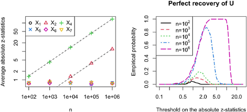
Following Section 3.2, we should be able to perfectly recover the set U (see, Equation (12)(12) $$\begin{array}{c}V=\left\{j:{\beta }_j^{\text{OLS}}={\beta }_j\right\}\hspace{1em}\text{and}\\ U=\left\{j:{\beta }_j^{\text{OLS}}={\beta }_j^{\text{HOLS}}\right\}=\left\{j:H_{0,j}\text{\hspace{0.17em}is}\mathrm{ }\text{true}\right\}.\end{array}$$(12) ) as $n\to \infty$ if we let the threshold on the absolute z-statistics grow at the right rate. Therefore, we plot on the right-hand side of Figure 2 the empirical probability of perfectly recovering U over a range of possible thresholds for the different sample sizes. For $n={10}^6$, we could achieve an empirical probability of 1. For $n={10}^5$ the optimum probability is 87%, while as for $n={10}^4$ it is only 19%.

Naturally, perfectly recovering U is a very ambitious goal for smaller sample sizes, and one might want to consider different objectives. In Figure 3, we plot two different performance metrics. On the left-hand side, we plot the empirical probability of not falsely including any variable in $\widehat{U}$ against the average intersection size $\left|\widehat{U}\cap U\right|$. The curve is parameterized implicitly by the threshold on the absolute z-statistics in order to reject the local null hypothesis for some variable. Thus, the graphic considers the question of how many variables in U can be recovered while keeping the probability of not falsely including any low. For a sample size of 10⁵, we have an average intersection size of 3.97 allowing for a 10% probability of false inclusions. For 10⁴, it is still 0.995. Thus, we can find (almost) one of the four variables in U on average. As we see in Figure 2, the bias on ${\beta }_4^{\text{OLS}}$ is much easier to detect than the bias on ${\beta }_2^{\text{OLS}}$. Thus, keeping the probability of including X₂ in $\widehat{U}$ low is still an ambitious task. Therefore, we analyze on the right-hand side of Figure 3 how many variables in U we can find while removing a certain amount of confounding signal. We define the remaining fraction as$$\frac{{\Vert {\mathit{\beta }}_{\widehat{U}}^{\text{OLS}}-{\mathit{\beta }}_{\widehat{U}}\Vert }_1}{{\Vert {\mathit{\beta }}^{\text{OLS}}-\mathit{\beta }\Vert }_1},$$that is, how much of the difference ${\mathit{\beta }}^{\text{OLS}}-\mathit{\beta }$ persists in terms of ${\mathcal{l}}_1$ norm.

Fig. 3 Simulation in a linear SEM corresponding to Figure 1. The results are based on 200 simulation runs. On the left: Probability of not falsely including a variable in $\widehat{U}$ versus average intersection size $\left|\widehat{U}\cap U\right|$ (see, Equation (14)(14) $$\widehat{U}=\left\{j:H_{0,j}\text{\hspace{0.17em}not}\mathrm{ }\text{rejected}\right\}$$(14) ). On the right: average remaining fraction of confounding signal versus average intersection size $\left|\widehat{U}\cap U\right|$. It holds that $\left|U\right|=4$. Both curves use the threshold on the absolute z-statistics as implicit curve parameter. Note that the legend applies to either plot.

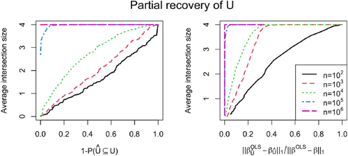
In this SEM, ${\beta }_4^{\text{OLS}}$ caries 2/3 of the confounding signal, ${\beta }_2^{\text{OLS}}$ only 1/3. Accepting 1/3 of remaining confounding signal, we receive an average intersection size of 3.885 for a sample size of 10³. For 10⁴, the average is 4. Thus, if we allow for false inclusion of X₂ we can almost perfectly retrieve all of U for sample size 10³ already.

What if X includes descendants of Y? So far, we have only considered the case where X causally affects Y, but potentially, some of Y’s parents are missing leading to a confounding effect. However, another possibility for ${\mathit{\beta }}^{\text{OLS}}$ to not denote a causal effect is that there are descendants of Y amongst the predictors. The two different situations are depicted in Figure 4. The case with descendants in the set of predictors fits our theory from before if interpreted properly. If the model (4) for Y holds true using only the parents as predictors, Y can be naturally included in the assumed linear SEM for X in (15). Then, one can also think of $\mathcal{E}$ as an unobserved confounder. The Markov boundary of $\mathcal{E}$ with respect to the observed predictors is the same as the Markov boundary of Y. Of course, it holds $\mathit{\beta }={\mathit{\beta }}^{*}$, that is, ${\beta }_j=0\forall j\notin \text{PA}(Y)$. Using Theorem 9, we find$$\begin{array}{c}{\beta }_j^{\text{HOLS}}={\beta }_j^{\text{OLS}}={\beta }_j=0\forall j\in M\hspace{1em}\text{that}\mathrm{ }\text{are}\mathrm{ }\text{not}\mathrm{ }\text{in}\mathrm{ }\text{the}\\ \hspace{1em}\hspace{1em}\hspace{1em}\text{Markov}\mathrm{ }\text{boundary}\mathrm{ }\text{of}\mathrm{ }Y.\end{array}$$

Fig. 4 Left: SEM with a hidden confounder. Right: SEM with a descendant of Y.

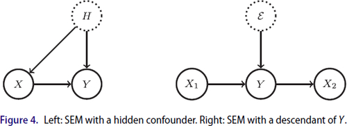
Thus, for all variables outside Y’s Markov boundary, one can correctly detect that they have no causal effect onto Y ceteris paribus. The coefficients for the variables in the boundary, which includes all parents, are up to term cancelations all subject to confounding bias. This can be detected under some conditions, as discussed in Section 3.2.

4.3 Beyond Linearity

We have mainly focused on linear models, that is, the data is either generated by model (4) or model (8). Naturally, this assumption might be questionable in practice. Therefore, we provide some intuition about how HOLS might be applied in a more general setup. As we only detect misspecification of the OLS coefficient without identifying the type of misspecification, one should not try to over-interpret the effect of the regressors in ${\widehat{U}}^c=\left\{1,\dots ,p\right\}\setminus \widehat{U}$ (see, Section 3.2). However, the linear effect of the variables in $\widehat{U}$ can always be interpreted to be well-specified, meaning that $\mathbb{E}\left[W_j|Z_j\right]=Z_j{\beta }_j^{\text{OLS}}$ or at least “sufficiently” well-specified such that no misspecification is detected in the data. Generally, we can write$$\begin{array}{c}Y={\mathbf{X}}^{\top }{\mathit{\beta }}^{\text{OLS}}+f_{\text{nonlinear}}\left(\mathbf{X}\right)+\mathcal{E},\text{\hspace{0.17em}where}\\ f_{\text{nonlinear}}\left(\mathbf{X}\right)=\mathbb{E}\left[Y|X\right]-{\mathbf{X}}^{\top }{\mathit{\beta }}^{\text{OLS}},\mathbb{E}\left[\mathcal{E}|\mathbf{X}\right]=0.\\ W_j=Z_j{\beta }_j^{\text{OLS}}+f_{\text{nonlinear}}\left(\mathbf{X}\right)+\mathcal{E}.\end{array}$$

Thus, well-specification of ${\beta }_j^{\text{OLS}}$ implies $\mathbb{E}\left[f_{\text{nonlinear}}(\mathbf{X})|Z_j\right]=0$, that is, after linearly adjusting for ${\mathbf{X}}_{-j}$, X_j does not have any predictive power for $f_{\text{nonlinear}}(X)$. If it does not have any predictive power after linear adjustment, it would be a natural conclusion that it does not have predictive power after optimally adjusting for ${\mathbf{X}}_{-j}$ implying that $f_{\text{nonlinear}}(\mathbf{X})$ can be written as function of ${\mathbf{X}}_{-j}$ only. This would then imply$$\begin{array}{c}\mathbb{E}\left[Y|X_j=x_j+1,{\mathbf{X}}_{-j}={\mathbf{x}}_{-j}\right]-\mathbb{E}\left[Y|X_j=x_j,{\mathbf{X}}_{-j}={\mathbf{x}}_{-j}\right]\\ ={\beta }_j^{\text{OLS}}\hspace{1em}\forall x_j,{\mathbf{x}}_{-j}.\end{array}$$

Except for Gaussian data, such a linear relationship must be either causal or due to very pathological data setups. Excluding such unusual cancelations, the conclusion is that for $j\in U$ there must be a true linear causal effect from X_j to Y keeping the other predictors fixed, which can be consistently estimated using OLS. Of course, if there are no locally linear structures, it might well be that $U=\varnothing$ such that the local tests are not more informative than the global test. However, there is also nothing to be lost by exploiting this local view.

Note that the asymptotic results presented in Sections 3.1 and 3.2 hold for nonlinear data as well since they only assume model (10)–(11), which is the most general formulation.

5 Real Data Example

We analyze the flow cytometry dataset presented by Sachs et al. (2005). It contains cytometry measurements of 11 phosphorylated proteins and phospholipids. There is a “ground truth” on how these quantities affect each other, the so-called consensus network (Sachs et al. 2005). Data is available from various experimental conditions, some of which are interventional environments. The dataset has been further analyzed in various projects, see, for example, Mooij and Heskes (2013), Meinshausen et al. (2016), and Taeb et al. (2021). Following these works, we consider data from eight different environments, seven of which are interventional. The sample size per environment ranges from 707 to 913.

In our analysis, we focus on the consensus network from Sachs et al. (2005). For each node, we go through all environments, fit a linear model using all its claimed parents as predictors, and assess the goodness of fit of the model using our HOLS check. In the consensus network, there is one bidirected edge between the variables PIP2 and PIP3. We include it as a parent for either direction. For each suggested edge, we also collect the p-values from the linear model fit in all environments, keeping only those where the edge passes the local HOLS check at level $\alpha =5\%$ without multiplicity correction. We omit the multiplicity correction here to lower the tendency to falsely claim causal detection. In Table 1, we report the minimum p-value from OLS, over the environments where the HOLS check is passed, sorted by increasing p-values. Additionally, we show the number of environments in which the check is passed and out of these the number where the edge is significant at level $\alpha =5\%$ in the respective linear model fit (with Bonferroni correction over all 8 environments and 17 edges, that is, we require a p-value of at most $0.05/136$). Note that there is one p-value 0 reported corresponding to a t-value of 174, which exceeds the precision that can be obtained with the standard R-function lm.

Table 1 The working model is taken from the consensus network.

Edge	Passing HOLS	Significant in linear model	Minimum p-value
RAF → MEK	3	2	0
PKA → Akt	3	3	1.5e-120
PKA → Erk	5	5	3.8e-69
PKC → JNK	3	3	5.9e-55
PIP2 → PIP3	1	1	6.5e-40
PIP3 → PLCg	5	1	1.4e-36
PKC → p38	1	1	7.1e-34
PIP3 → PIP2	1	1	9.6e-08
PLCg → PKC	6	0	0.016
PLCg → PIP2	1	0	0.027
PKC → RAF	8	0	0.046
PKC → PIP2	8	0	0.057
PKA → RAF	8	0	0.086
PKA → p38	8	0	0.12
PIP3 → Akt	8	0	0.2
PKA → JNK	8	0	0.21
MEK → Erk	8	0	0.42

NOTE: The second column reports the number of environments in which the edge passes the HOLS check (among eight possible ones). The third column additionally shows, in how many of these it is also significant in the respective linear model fit. The p-value is the minimum of the p-values from linear regression in environments, where the edge passes the HOLS check.

We see that the edge RAF → MEK is the most significant. Further, every edge of the consensus network passes the HOLS check in at least one environment. Frequently, we see that edges pass the HOLS check in certain environments without being significant in the linear model. Considering our discussion around linear SEMs, this could easily happen if the alleged predictor node is not actually in the Markov boundary of the response. In fact, there are seven edges that pass the HOLS check in every environment which are not significant based on the linear model fits. This is in agreement with Taeb et al. (2021), where none of them is reported.

As we cannot guarantee that the data follows a linear SEM as in Equation (15)(15) $$X_j\leftarrow {\Psi }_j+\sum _{k\in \text{PA}\left(j\right)}{\theta }_{j,k}{X}_k\hspace{1em}j=1,\dots ,p,$$(15) , we shall not interpret the edges that do not pass the HOLS check to be subject to hidden confounding. However, the fact that we still find a decent number of suggested edges that pass the HOLS check, at least in some environments, leads to evidence that the assumption of some local unconfounded linear structures is not unrealistic, see also the discussion in Section 4.3.

We can also analyze our results in the light of invariant causal prediction, see, for example, Peters, Bühlmann, and Meinshausen (2016), where one typically assumes that interventions do not change the underlying graph except for edges that point toward the node that is intervened on. This assumption is highly questionable in practice, and our findings, which vary a lot over different environments, indicate that the assumption is likely not fulfilled in the given setup.

6 Discussion

We have introduced the so-called HOLS check to assess the goodness of fit of linear causal models. It is based on the dependence between residuals and predictors in misspecified models, leading to nonvanishing higher moments. Besides checking whether the overall model might hold true, the method allows to detect a set of variable for which linear regression consistently estimates a true (unconfounded) causal effect for certain model classes.

We extend the HOLS method to high-dimensional datasets based on the idea of the debiased Lasso (Zhang and Zhang 2014; van de Geer et al. 2014). This extension comes very naturally as our HOLS check involves nodewise regression just as the debiased Lasso.

Of particular interest are linear structural equation models, for which our method allows for very precise characterizations regarding which least squares parameters are causal effects. The result requires some non-Gaussianity. We complement our theory with a simulation study as well as a real data example.

A drawback of our method is that it does not distinguish whether a model is misspecified due to confounding or due to nonlinearities in the model. Therefore, an interesting follow-up direction would be to extend our methodology and theory from linear to nonlinear SEM using more flexible regression methods. This could allow to detect local causal structures in nonlinear settings as well.

Supplementary Materials

Simulation results as well as proofs and extended theory can be found in the supplemental material.

Data Availability Statement

Code scripts to reproduce the results presented in this article are available here https://github.com/cschultheiss/HOLS.

Disclosure Statement

The authors report there are no competing interests to declare.

Additional information

Funding

The project leading to this application has received funding from the European Research Council (ERC) under the European Union’s Horizon 2020 research and innovation programme (grant agreement No 786461). M. Yuan was supported in part by NSF Grants DMS-2015285 and DMS-2052955. Part of the work was done while M. Yuan was visiting the Institute for Theoretical Studies at ETH Zürich, Switzerland, and he wishes to thank the institute for their support and hospitality.

References

- Angrist, J. D., Imbens, G. W., and Rubin, D. B. (1996), “Identification of Causal Effects using Instrumental Variables,” Journal of the American Statistical Association, 91, 444–455. DOI: 10.1080/01621459.1996.10476902.
- Belsley, D. A., Kuh, E., and Welsch, R. E. (2005), Regression Diagnostics: Identifying Influential Data and Sources of Collinearity, Hoboken, NJ: Wiley.
- Bowden, R. J., and Turkington, D. A. (1990), Instrumental Variables, Cambridge: Cambridge University Press.
- Bühlmann, P. (2013), “Statistical Significance in High-Dimensional Linear Models,” Bernoulli, 19, 1212–1242. DOI: 10.3150/12-BEJSP11.
- Buja, A., Brown, L., Berk, R., George, E., Pitkin, E., Traskin, M., Zhang, K., and Zhao, L. (2019a), “Models as Approximations I: Consequences Illustrated with Linear Regression,” Statistical Science, 34, 523–544. DOI: 10.1214/18-STS693.
- Buja, A., Brown, L., Kuchibhotla, A. K., Berk, R., George, E., and Zhao, L. (2019b), “Models as Approximations II: A Model-Free Theory of Parametric Regression,” Statistical Science, 34, 545–565. DOI: 10.1214/18-STS694.
- Ćevid, D., Bühlmann, P., and Meinshausen, N. (2020), “Spectral Deconfounding via Perturbed Sparse Linear Models,” Journal of Machine Learning Research, 21, 9442–9482.
- Godfrey, L. G. (1991), Misspecification Tests in Econometrics: The Lagrange Multiplier Principle and Other Approaches, Cambridge: Cambridge University Press.
- Greene, W. H. (2003), Econometric Analysis, Noida: Pearson Education India.
- Guo, Z., Ćevid, D., and Bühlmann, P. (2022), “Doubly Debiased Lasso: High-Dimensional Inference Under Hidden Confounding,” Annals of Statistics, 50, 1320–1347. DOI: 10.1214/21-aos2152.
- Hausman, J. A. (1978), “Specification Tests in Econometrics,” Econometrica: Journal of the Econometric Society, 46, 1251–1271. DOI: 10.2307/1913827.
- Hoyer, P. O., Hyvärinen, A., Scheines, R., Spirtes, P., Ramsey, J., Lacerda, G., and Shimizu, S. (2008), “Causal Discovery of Linear Acyclic Models with Arbitrary Distributions,” in Proceedings of the Twenty-Fourth Conference on Uncertainty in Artificial Intelligence, pp. 282–289.
- Hyvärinen, A., and Oja, E. (2000), “Independent Component Analysis: Algorithms and Applications,” Neural Networks, 13, 411–430. DOI: 10.1016/s0893-6080(00)00026-5.
- Imbens, G. W., and Rubin, D. B. (2015), Causal Inference in Statistics, Social, and Biomedical Sciences, New York: Cambridge University Press.
- Lehmann, E. L., Romano, J. P., and Casella, G. (2005), Testing Statistical Hypotheses (Vol. 3), Cham: Springer.
- Maddala, G., and Lahiri, K. (2009), Introduction to Econometrics (4th ed), Chichester: Wiley.
- Meinshausen, N., Hauser, A., Mooij, J. M., Peters, J., Versteeg, P., and Bühlmann, P. (2016), “Methods for Causal Inference from Gene Perturbation Experiments and Validation,” Proceedings of the National Academy of Sciences, 113, 7361–7368. DOI: 10.1073/pnas.1510493113.
- Mooij, J. M., and Heskes, T. (2013), “Cyclic Causal Discovery from Continuous Equilibrium Data,” in Proceedings of the Twenty-Ninth Conference on Uncertainty in Artificial Intelligence, pp. 431–439.
- Peters, J., Bühlmann, P., and Meinshausen, N. (2016), “Causal Inference by using Invariant Prediction: Identification and Confidence Intervals,” Journal of the Royal Statistical Society, Series B, 78, 947–1012. DOI: 10.1111/rssb.12167.
- Peters, J., Mooij, J. M., Janzing, D., and Schölkopf, B. (2014), “Causal Discovery with Continuous Additive Noise Models,” Journal of Machine Learning Research, 15, 2009–2053.
- Sachs, K., Perez, O., Pe’er, D., Lauffenburger, D. A., and Nolan, G. P. (2005), “Causal Protein-Signaling Networks Derived from Multiparameter Single-Cell Data,” Science, 308, 523–529. DOI: 10.1126/science.1105809.
- Shah, R. D., and Bühlmann, P. (2018), “Goodness-of-Fit Tests for High Dimensional Linear Models,” Journal of the Royal Statistical Society, Series B, 80, 113–135. DOI: 10.1111/rssb.12234.
- Shimizu, S., Hoyer, P. O., Hyvärinen, A., Kerminen, A., and Jordan, M. (2006), “A Linear Non-Gaussian Acyclic Model for Causal Discovery,” Journal of Machine Learning Research, 7, 2003–2030.
- Taeb, A., Gamella, J. L., Heinze-Deml, C., and Bühlmann, P. (2021), “Perturbations and Causality in Gaussian Latent Variable Models,” arXiv preprint arXiv:2101.06950.
- van de Geer, S., Bühlmann, P., Ritov, Y., and Dezeure, R. (2014), “On Asymptotically Optimal Confidence Regions and Tests for High-Dimensional Models,” The Annals of Statistics, 42, 1166–1202. DOI: 10.1214/14-AOS1221.
- Wang, Y. S., and Drton, M. (2020), “High-Dimensional Causal Discovery under Non-Gaussianity,” Biometrika, 107, 41–59. DOI: 10.1093/biomet/asz055.
- Zhang, C.-H., and Zhang, S. S. (2014), “Confidence Intervals for Low Dimensional Parameters in High Dimensional Linear Models,” Journal of the Royal Statistical Society, Series B, 76, 217–242. DOI: 10.1111/rssb.12026.