
 ?Mathematical formulae have been encoded as MathML and are displayed in this HTML version using MathJax in order to improve their display. Uncheck the box to turn MathJax off. This feature requires Javascript. Click on a formula to zoom.
Abstract
We propose a new unsupervised learning method for clustering a large number of time series based on a latent factor structure. Each cluster is characterized by its own cluster-specific factors in addition to some common factors which impact on all the time series concerned. Our setting also offers the flexibility that some time series may not belong to any clusters. The consistency with explicit convergence rates is established for the estimation of the common factors, the cluster-specific factors, and the latent clusters. Numerical illustration with both simulated data as well as a real data example is also reported. As a spin-off, the proposed new approach also advances significantly the statistical inference for the factor model of Lam and Yao. Supplementary materials for this article are available online.
1 Introduction
One of the primary tasks of data mining is clustering. While most clustering methods are originally designed for independent observations, clustering a large number of time series gains increasing momentum (Esling and Agon, Citation2012), due to mining large and complex data recorded over time in business, finance, biology, medicine, climate, energy, environment, psychology, multimedia and other areas (Table 1 of Aghabozorgi, Shirkhorshid, and Wah, Citation2015). Consequently, the literature on time series clustering is large; see Liao (Citation2005), Aghabozorgi, Shirkhorshid, and Wah (Citation2015), Maharaj, D’Urso, and Caiado (Citation2019) and the references therein. The basic idea is to develop some relevant similarity or distance measures among time series first, and then to apply the standard clustering algorithms such as hierarchical clustering or k-means method. Most existing similarity/distances measures for time series may be loosely divided into two categories: data-based and feature-based. The data-based approaches define the measures directly based on observed time series using, for example, L2- or, more general, Minkowski’s distance, or various correlation measures. Alonso and Peña (Citation2019) proposed a generalized cross-correlation as a similarity measure, which takes into account cross-correlation over different time lags. Dynamic time warping can be applied beforehand to cope with time deformation due to, for example, shifting holidays over different years (Keogh and Ratanamahatana, Citation2005). The feature-based approaches extract relevant features from observed time series data first, and then define similarity/distance measures based on the extracted features. The feature extraction can be carried out by various transformations such as Fourier, wavelet or principal component analysis (sec. 2.3 of Roelofsen, Citation2018). The features from fitted time series models can also be used to define similarity/distance measures (Yao et al., Citation2000; Frühwirth-Schnatter and Kaufmann, Citation2008). Attempts have also been made to define the similarity between two time series by measuring the discrepancy between the two underlying stochastic processes (Kakizawa, Shumway, and Taniguchi, Citation1998; Khaleghi et al., Citation2016). Other approaches include Zhang (Citation2013) which clusters time series based on the parallelism of their trend functions, and Ando and Bai (Citation2017) which represents the latent clusters in terms of a factor model. So-called “subsequence clustering” occurs frequently in the literature on time series clustering; see Keogh and Lin (Citation2005) and Zolhavarieh, Aghabozorgi, and Teh (Citation2014). It refers to clustering the segments from a single long time series, which is not considered in this article.
The goal of this study is to propose a new factor model based approach to cluster a large number of time series into different and unknown clusters such that the members within each cluster share a similar dynamic structure, while the number of clusters and their sizes are all unknown. We represent the dynamic structures by latent common and cluster-specific factors, which are both unknown and are identified by the difference in factor strength. The strength of a factor is measured by the number of time series which influence and/or are influenced by the factor (Chamberlain, Citation1983). The common factors are strong factors as each of them carries the information on most (if not all) time series concerned. The cluster-specific factors are weak factors as they only affect the time series in a specific cluster.
Though our factor model is similar to that of Ando and Bai (Citation2017), our approach is radically different. First, we estimate strong factors and all the weaker factors in the manner of one-pass, and then the latent clusters are recovered based on the estimated weak factor loadings. Ando and Bai (Citation2017) adopted an iterative least squares algorithm to estimate factors/factor loadings and latent cluster structure recursively. Second, our setting allows the flexibility that some time series do not belong to any clusters, which is often the case in practice. Third, our setting allows the dependence between the common factors and cluster-specific factors while Ando and Bai (Citation2017) imposed an orthogonality condition between the two; see Remark 1(iv) in Section 2.
The methods used for estimating factors and factor loadings are adapted from Lam and Yao (Citation2012). Nevertheless substantial advances have been made even within the context of Lam and Yao (Citation2012): (i) we remove the artifact condition that the factor loading spaces for strong and weak factors are perpendicular with each other, (ii) we allow weak serial correlations in idiosyncratic components in the model, which were assumed to be vector white noise by Lam and Yao (Citation2012), and, more significantly, (iii) we propose a new and consistent ratio-based estimator for the number of factors (see Step 1 and also Remark 3(iii) in Section 3).
The rest of the article is organized as follows. Our factor model and the relevant conditions are presented in Section 2. We elaborate explicitly why it is natural to identify the latent clusters in terms of the factor strength. The new clustering algorithm is presented in Section 3. The clustering is based on the factor loadings on all the weak factors; applying a K-means algorithm using a correlation-type similarity measure defined in terms of the loadings. The asymptotic properties of the estimation for factors and factor loadings are collected in Section 4. Section 5 presents the consistency the proposed factor-based clustering algorithm with error rates. Numerical illustration with both simulated and a real data example is reported in Section 6. We also provide some comments in Section 7. All technical proofs are presented to a supplementary materials.
We always assume vectors in column. Let denote the Euclidean norm of vector
. For any matrix
, let
denote the linear space spanned by the columns of
the square root of the largest eigenvalue of
the square root of the smallest eigenvalue of
,
the matrix with
as its (i, j)th element. We write
if
and
. We use
to denote generic constants independent of p and n, which may be different at different places.
2 Models
Let be a weakly stationary
vector time series, that is,
is a constant independent of t, and all elements of
are finite and dependent on k only. Suppose that
consists of d + 1 latent segments, that is,
(1)
(1) where
are, respectively,
-vector time series with
, and
Furthermore, we assume the following latent factor model with d clusters:
(2)
(2) where
is a
matrix with rank r0,
is r0-vector time series representing r0 common factors and
is
matrix with rank rj,
is rj-vector time series representing rj factors for
only and
,
stands for a
matrix with all elements equal to 0,
, and
is an idiosyncratic component in the sense of Chamberlain (Citation1983) and Chamberlain, and Rothschild (Citation1983) (see below). Note that in the model above, we only observe permuted
(i.e., the order of components of
is unknown) while all the terms on the RHS of (2) are unknown.
By (2), the p0 components of are grouped into d clusters
, while the
components of
do not belong to any clusters. The jth cluster
is characterized by the cluster-specific factor
, in addition to the dependence on the common factor
. The goal is to identify those d latent clusters from observations
. Note that all pj, rj and d are also unknown.
We always assume that the number of the common factors and the number of cluster-specific factors for each cluster remain bounded when the number of time series p diverges. This reflects the fact that the factor models are only appealing when the numbers of factors are much smaller than the number of time series concerned. Furthermore, we assume that the number of time series in each cluster pi diverges at a lower order than p and the number of clusters d diverges as well. See Assumption 1.
Assumption 1.
,
, and
for
, where C > 0 and
are constants independent of n and p.
The strength of a factor is measured by the number of time series which influence and/or are influenced by the factor. Each component of is a common factor. It is related to most, if not all, components of
in the sense that the most elements of the corresponding column of
(i.e., the factor loadings) are nonzero. Hence, it is reasonable to assume
(3)
(3) where
is the jth column of
. This is in the same spirit of the definition for the common factors by Chamberlain, and Rothschild (Citation1983). Denoted by
the ith column of the
matrix
. In the same vein, we assume that
(4)
(4)
as each cluster-specific factor for the jth cluster is related to most of the
(Assumption 1) time series in the cluster. Note that the factor strength can be measured by constant
:
in (4) indicates that factors
are weaker than factors
which corresponds to δ = 0; see (3).
Conditions (3) and (4) are imposed under the assumption that all the factors remain unchanged as p diverges, all the entries of covariance matrices below are bounded,
and, furthermore,
and
are full-ranked for
, where
is an integer. Then conditions (3) and (4) are equivalent to (6) and (7) in Assumption 3 after the orthogonal normalization to be introduced now in order to make model (2) partially identifiable and operationally tractable.
In model (2) and
are not uniquely defined, as, for example,
can be replaced by
for any
invertible matrix
. We argue that this lack of uniqueness gives us the flexibility to choose appropriate
and
to facilitate our estimation more readily. Assumption 2 specifies both
and
to be half-orthogonal in the sense that the columns of
or
are orthonormal, which can be fulfilled by, for example, replacing the original
by
, where
is a QR decomposition of
. Even under Assumption 2,
and
are still not unique. In fact that only the factor loading spaces
are uniquely defined by (2). Hence
, that is, the projection matrix onto
, is also unique.
Assumption 2.
for
, and it holds for a constant
that
(5)
(5)
Furthermore for ,
cannot be written as a block diagonal matrix with at least two blocks, where
denotes any row-permutation of
.
Condition (5) implies that the columns of do not fall entirely into the space
as otherwise one cannot distinguish
from
. It is automatically fulfilled if
which is a condition imposed in Lam and Yao (Citation2012). Finally the last condition in Assumption 2 ensures that the number of clusters d is uniquely defined.
Assumption 3.
Let , and
be strictly stationary with the finite fourth moments. As
, it holds for
that
(6)
(6)
(7)
(7)
(8)
(8)
(9)
(9)
Furthermore, is ψ-mixing with the mixing coefficients satisfying
, and
,
for any t and s.
Remark 1.
(i) The factor strength is defined in terms of the orders of the factor loadings in (3) and (4). Due to the orthogonalization specified in Assumption 2, they are transformed into the orders of the covariance matrices in (6) and (7). See also Remark 1 in Lam and Yao (Citation2012). Nevertheless, the factor strength is still measured by the constant : the smaller δ is, the stronger a factor is. The common factors in
are the strongest with δ = 0, and the cluster-specific factors in
are weaker with
. In (2)
represents the idiosyncratic component of
in the sense that each component of
only affects the corresponding component and a few other components of
(i.e., δ = 1), which is implied by Assumptions 4. Hence, the strength of
is the weakest. The differences in the factor strength make
, and
on the RHS of (2) (asymptotically) identifiable. To simplify the presentation, we assume that all the components of
are of the same strength (i.e., all pi are of the same order). See the real data example in Section 6.2 for how to handle the cluster-specific factors of different strengths.
(ii) Model (2) is similar to that of Ando and Bai (Citation2017). However, we do not require that the common factor and the cluster-specific factor
are orthogonal with each other in the sense that
, which is imposed by Ando and Bai (Citation2017). Furthermore, we allow the idiosyncratic term
to exhibit weak autocorrelations (Assumption 4), instead of complete independence as in Ando and Bai (Citation2017).
We now impose some structure assumptions on the idiosyncratic term in model (2).
Assumption 4.
Let , where
is a p × p constant matrix with
bounded from above by a positive constant independent of p. Furthermore, one of the following two conditions holds.
is MA(
Remark 2.
In Assumption 4, (i) assumes that is a linear process with the same serial correlation structure across all the components. (ii) allows some nonlinear serial dependence, the dependence structures for different components may differ. But then the sub-Gaussian condition (10) is required.
3 A Clustering Algorithm
With available observations , we propose below an algorithm (in five steps) to identify the latent d clusters. To this end, we introduce some notation first. Let
,
(11)
(11) where
is a pre-specified integer in Assumption 3.
Step 1(Estimation for the number of factors.) For
Step 2(Estimation for the loadings for common factors.) Let
Step 3(Estimation for the loadings for cluster-specific factors.) Replace
Step 4(Identification for the components not belonging to any clusters.) Let
Step 5 (K-means clustering.) Denote by
Perform the K-means clustering (with L2-distance) for the rows of
to form the d clusters, where
is chosen such that the within-cluster-sum of L2-distances (to the cluster center points) are stabilized.
Remark 3.
(i) The ratio-based estimation in Step 1 is new. By Theorem 3 in Section 4, it holds and
in probability. The existing approaches use the ratios of the ordered eigenvalues of matrix
instead (Lam and Yao, Citation2012; Chang, Gao, and Yao, Citation2015; Li, Wang, and Yao, Citation2017); leading to an estimator which may not be consistent. See Example 1. Note that Lam and Yao (Citation2012) shows that their estimator
fulfills the relation
only.
(ii) The intuition behind the estimators in (12) is that the eigenvalues of matrix
, where
, satisfy the conditions
This is implied by the differences in strength among the common factor , the cluster specific factors
, and the idiosyncratic components
; see Theorem 3. Note that we use the ratios of the cumulative eigenvalues in (12) in order to add together the information from different lags k. In practice, we set k0 to be a small integer such as
, as the significant autocorrelation occurs typically at small lags. The results do not vary that much with respect to the value of k0 (see the simulation results in Section 6.1). We truncate the sequence
at J0 to alleviate the impact of “0/0”. In practice, we may set
or
.
(iii) Step 3 removes the common factors first before estimating , as Lam and Yao (Citation2012) showed that weak factors can be more accurately estimated by removing strong factors from the data first.
(iv) Once the numbers of strong and weak factors are correctly specified, the factor loading spaces are relatively easier to identify. In fact is a consistent estimator for
. However,
is a consistent estimator for
instead of
. See Theorem 2 in Section 4. Furthermore the last
rows of
are no longer 0. Nevertheless when the elements in
and
have different orders, those
zero-rows can be recovered from
in Step 4. See Theorem 5 in Section 5.
(v) Given the block diagonal structure of in (2), the d clusters would be identified easily by taking the (i, j)th element of
as the similarity measure between the ith and the jth components, or by simply applying the K-means method to the rows of
. However, applying the K-means method directly to the rows of
will not do. Theorems 2 and 4 indicate that the block diagonal structure, though masked by asymptotically diminishing “noise”, still presents in
via a latent row-permutation of
. Accordingly the cluster analysis in Step 5 is based on the absolute values of the correlation-type measures among the rows of
which is an estimator for
.
(vi) In Step 5, we search for the number of clusters d by the “elbow method” which is the most frequently used method in K-means clustering. Nevertheless provides an upper bound for d; see Theorem 6. Our empirical experiences indicate that
holds often especially when rj,
, are small. See Tables 7 and 8 in Section 6.1. Note that
is a block diagonal matrix with d blocks and all the nonzero eigenvalues equal to 1. Therefore the dominant eigenvalue for each of the latent d blocks in
is greater than or at least very close to 1. Moreover, by Perron-Frobenius’s theorem, the largest eigenvalue of
, that is, the so-called Perron-Frobenius eigenvalue, is strictly greater than the other eigenvalues of
under the last condition in Assumption 2. This is the intuition behind the definition of
.
Example 1.
Consider a simple model of the form (2) in which and
where
are constants, and
, for different i, t, are independent and N(0, 1). Let
, and
be the three largest eigenvalues of
. It can be shown that
and
provided
. Hence,
. This shows that
or
cannot be estimated stably based on the ratios of the eigenvalues of
for this example. In fact, let two
matrices
and
be the eigenvectors of
and
. When
and
are different while
.
4 Asymptotic Properties on Estimation for Factors
Theorem 1 and Remark 4 show that in the absence of weak factor , the estimation for the strong factor loading space
achieves root-n convergence rate in spite of diverging p. Since only the factor loading space
is uniquely defined by (2) (see the discussion below Assumption 2), we measure the estimation error in terms of its (unique) projection matrix
.
Theorem 1.
Let Assumptions 1–4 hold. Let and
. Then it holds that
(17)
(17)
Assumption 2 ensures that the rank of matrix is r. Denote by
the projection matrix onto
of which
is a consistent estimator, see Theorem 2, and also Remark 3(iv).
Theorem 2.
Let Assumptions 1–4 hold. Let . Then it holds that
(18)
(18)
and
(19)
(19)
Theorem 3 specifies the asymptotic behavior for the ratios of the cumulated eigenvalues used in estimating the numbers of factors in Step 1 in Section 3. It implies that in probability provided that
is fixed.
Theorem 3.
Let Assumptions 1–4 hold. Let . For
defined in (12), it holds for some constant C > 0 that
(20)
(20)
(21)
(21)
(22)
(22)
(23)
(23) where s is a positive fixed integer.
Remark 4.
It is worth pointing out that the block diagonal structure of is not required for Theorems 1–3. On the other hand, if
and
and
are independent, the term
on the RHS of (17)–(19) disappears.
5 Asymptotic Properties on Clustering
Assumption 5.
The elements of are of the order
, and
for
, where
denotes the ith row of matrix
.
The orthogonalization implies that the average of the squared elements of
is
. Since r0 is finite, it is reasonable to assume that the elements of
are
. As
is a block-diagonal matrix with blocks
and
, the squared elements of
are of the order
in average. As rj is bounded, it is reasonable to assume
. Assumption 5 ensures that
is asymptotically a block diagonal matrix; see Theorem 4. This enables to recover the block diagonal structure of
based on
which provides a consistent estimator for the space
(Theorem 2), and also to separate the components of
not belonging to any clusters. See Theorems 5–7 .
Theorem 4.
Let Assumptions 1–2 and 5 hold. Divide matrix into
blocks, and denote its (i, j)th block of the size
by
. Then as
,
.
Theorem 5.
Let the conditions of Theorem 2 and Assumption 5 hold. For defined in (16), it holds that
(24)
(24)
(25)
(25) where ωp is given in (16). Furthermore,
provided that
.
Theorem 6.
Let the conditions of Theorem 5 hold, and . Then
as
.
Remark 5.
Theorem 5 shows that most the components belonging to the d clusters will not be classified as not belonging to any clusters (see (24)). Furthermore most the components not belonging to any clusters will be correctly identified (see (25)). Theorem 6 shows that the probability of under-estimating d converges to 0.
To investigate the errors in the K-means clustering, let be the
matrix with
We assume that d is known. Let be the set consisting of all
matrices with d distinct rows. Put
(26)
(26)
For any p0-vector with its elements taking integer values between 1 and d, let
Note that the d distinct rows of would be the centers of the d clusters identified by the K-means method based on the rows of
. However
is unknown, we identify the d clusters based on its estimator
; see Step 5 of the algorithm in Section 3. The clustering based on
can only be successful if that based on
is successful, that is,
, where
is the p0-vector with 1 as its first p1 elements, 2 as its next p2 elements,
, and d as its last pd elements. Given the block diagonal structure of
, condition
is likely to hold.
For any p0-vector with its elements taking integer values between 1 and d, it partitions
into d subset. Let
denote the number of misclassified components by partition g.
Assumption 6.
. For some constant c > 0,
Theorem 7.
Let the conditions of Theorem 5 and Assumption 6 hold. The number of clusters d is assumed to be known. Denoted by the number of misclassified components of
by the K-means clustering in Step 5. Then as
,
(27)
(27)
Remark 6.
Theorem 7 implies that the misclassification rate of the K-means method converges to 0, though the convergence rate is slow (see (27)). However, a faster rate is attained when , and
and
are independent, as then
. See also Remark 4. Assumption 6 requires that
increases as the number of misplaced members of this partition
becomes large, which is necessary for the K-means method.
6 Numerical Properties
6.1 Simulation
We illustrate the proposed methodology through a simulation study with model (2). We draw the elements of and
independently from
. All component series of
and
are independent and AR(1) and MA(1), respectively, with Gaussian innovations. All components of
are independent MA(1) with
innovations. All the AR and the MA coefficients are drawn randomly from
. The standard deviations of the components of
and
are drawn randomly from U(1, 2).
We consider following two scenarios with and
:
Scenario I: n = 400, d = 5 and
Scenario II: n = 800, d = 10 and
The numbers of factors r0 and r are estimated based on the ratios in (13) with
and
in (12). For the comparison purpose, we also report the estimates based on the ratios of eigenvalues of
in (11) also with
, which is the standard method used in literature and is defined as in (13) but now with
instead, where
are the eigenvalues of
. See, for example, Lam and Yao (Citation2012). For each setting, we replicate the experiment 1000 times.
The relative frequencies of and
are reported in . Overall the method based on the ratios of the cumulative eigenvalues
provides accurate and robust performance and is not sensitive to the choice of k0. The estimation based on the eigenvalues of
with
is competitive for r0, but is considerably poorer for
in Scenario II. Using
with k = 0 leads to weaker estimates for r0 in Scenario I.
Table 1 The relative frequencies of and
in a simulation for Scenario I with 1000 replications, where
and
are estimated by the
-based method (13), and the ratios of the eigenvalues of
.
Table 2 The relative frequencies of and
in a simulation for Scenario II with 1000 replications, where
and
are estimated by the
-based method (13), and the ratios of the eigenvalues of
.
It is noticeable that the performance of the estimation for the number of common factor r0 in Scenario II is better than Scenario I. This is due to the fact the difference in the factor strength between the common factor and the cluster-based factor
in Scenario II is larger than Scenarios I. In contrast, the results hardly change with different values of p1.
Recall is the projection matrix onto the space
; see Theorem 2 and also Remark 3(iv). contain the means and standard deviations of the estimation errors for the factor loading spaces
and
, where
is estimated by the eigenvectors of the matrix
in (11) with
, see Step 2 of the algorithm stated in Section 3. See also Step 3 there for the similar procedure in estimating
. For the comparison purpose, we also include the estimates obtained with
replaced by
with
. show clearly that the estimation based on
is accurate and robust with respect to the different values of k0. Furthermore using a single-lagged covariance matrix for estimating factor loading spaces is not recommendable. The error
in Scenario I is larger than the error in Scenarios II. This is due to the larger sample size n in Scenario II. See Theorem 1. In contrast, Theorem 2 shows that the error rate of
contains the term
. While n is larger in Scenario II, so is
. This explains why the error
in Scenario II is also larger than that in Scenario I.
Table 3 The means and standard deviations (in parentheses) of and
in a simulation for Scenario I with 1000 replications, where
is estimated by the eigenvectors of
in (11) (with
), or by those of
(for
), and
is estimated in the similar manner.
Table 4 The means and standard deviations (in parentheses) of and
in a simulation for Scenario II with 1000 replications, where
is estimated by the eigenvectors of
in (11) (with
), or by those of
(for
), and
is estimated in the similar manner.
In the sequel, we only report the results with and
estimated by (13), and the factor loading spaces estimated by the eigenvectors of
. We always set
. We examine now the effectiveness of Step 4 of the algorithm. Note that the indices of the components not belonging to any clusters are identified as those in
in (16), which is defined in terms of a threshold
. We experiment with the three choices of this tuning parameter, namely
,
and
. Recall
contains all the indices of the components of
belonging to one of the d clusters. The means and standard deviations of the two types of misclassification errors
and
over the 1000 replications are reported in . Among the three choices,
appears to work best as the two types of errors are both small. The increase in the errors due to the estimation for r0 and r is not significant.
Table 5 The means and standard deviations (in parentheses) of the error rates and
in a simulation for Scenario I with 1000 replications with the three possible choices of threshold ωp in (16), and the numbers of factors r0 and r either known or to be estimated.
Table 6 The means and standard deviations (in parentheses) of the error rates and
in a simulation for Scenario II with 1000 replications with the three possible choices of threshold ωp in (16), and the numbers of factors r0 and r either known or to be estimated.
In the sequel, we only report the results with . In Step 5, we estimate
as an upper bound for d. As rj = 2 for
occurs almost surely in our simulation. See . Then the
clusters are obtained by performing the K-means clustering for the
rows of
, where
. As the error rates in estimating
has already been reported in , we concentrate on the components of
with indices in
now, and count the number of them which were misplaced by the K-means clustering, that is,
. Both the means and the standard deviations of the error rates
over 1000 replications are reported in . We also report the relative frequencies of
. show clearly that the K-means clustering identifies the latent clusters very accurately, and the difference in performance due to the estimating
is also small.
Table 7 The means and Standard Deviations (STD) of the error rates and the relative frequencies of
in a simulation for Scenario I with 1000 replications with the numbers of factors r0 and r either known or to be estimated.
Table 8 The means and Standard Deviations (STD) of the error rates and the relative frequencies of
in a simulation for Scenario II with 1000 replications with the numbers of factors r0 and r either known or to be estimated.
6.2 Real Data Illustration
We consider the daily returns of the stocks listed in S&P500 in December 31, 2014–December 31, 2019. By removing those which were not traded on every trading day during the period, there are p = 477 stocks which were traded on n = 1259 trading days. Those stocks are from 11 industry sectors:
The conventional wisdom suggests that the companies in the same industry sector share some common features. We apply the proposed 5-step algorithm in Section 3 to the return series to cluster those 477 stocks into different groups.
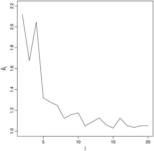
Step 1 is to estimate the numbers of strong factors and cluster-specific weak factors. To this end, we calculate as in (12) with
. It turns out
is much larger than all the others, while
for
are plotted in . By (13),
and
. Note that the estimates for
and
are unchanged with
. While the existence of
strong and common factor is reasonable, it is most unlikely that there are merely
cluster-specific weak factors. Note that estimators in (13) are derived under the assumption that all the r cluster-specific (i.e., weak) factors are of the same factor strength; see Remark 1(ii) in Section 2. In practice weak factors may have different degrees of strength; implying that we should also take into account the 3rd, the 4th, the 5th largest local maximum of
. Hence, we take
(or perhaps also 10 or 13), as suggests that there are 3 factors with factor strength
, and further 12 factors with strength
.
Fig. 1 Plot of against j for
.
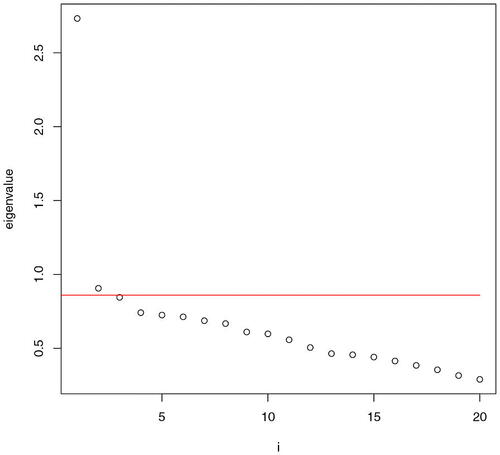
With and
, we proceed to Steps 2 & 3 of Section 3 and obtain the estimator
as in (15). Setting
,
, that is, 11 stocks do not appear to belong to any clusters, where
is defined as in (16) in Step 4. Leaving those 11 stocks out, we perform Step 5, that is, the K-means clustering for the
rows of matrix
. From we choose
. But we also consider
and
as two more examples.
Fig. 2 The eigenvalues of when
and
. The red line is
.
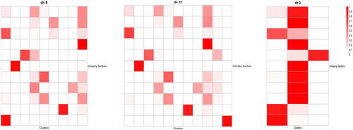
To present the identified d clusters, we define matrix with
as its (i, j)th element, where ni is the number of the stocks in the ith industry sector, and nij is the number of the stocks in the ith industry sector which are allocated in the jth cluster. Thus,
and
.
The heat-maps of this matrix for
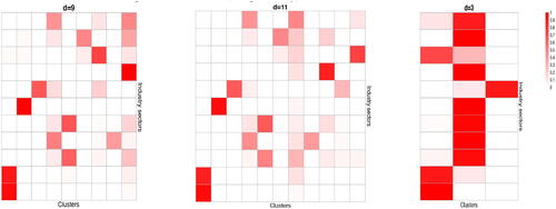
is presented in . The first cluster mainly consists of the companies in Consumer Staples, and Utilities, Clusters 2 and 3 contain the companies in, respectively, Health Care and Financials, Cluster 4 contains mainly some companies in Communication Service and Information Technology, Cluster 5 consists of the companies in Industrials and Materials, Cluster 6 are mainly the companies in Consumer Discretionary, Cluster 7 are mainly the companies in Real Estate. Cluster 8 is mainly the companies from Information Technology, Cluster 9 contains almost all companies in Energy and a small number of companies from each of 5 or 6 different sectors. To examine how stable the clustering is, we also include the results for d = 11 and d = 3 in . When d is increased from 9 to 11, the original Cluster 1 is divided into new Clusters 1 and 11 with the former consisting of Consumer Staples, and the latter being Utilities. Furthermore the original Cluster 4 splits into new Clusters 4 and 10, while the other 7 original clusters are hardly changed. With d = 3, most companies in each of the 11 sectors stay in one cluster. For example, most companies in Financials are always in a separate group.
Fig. 3 Heat-maps of the distributions of the stocks in each of the 11 industry sectors (corresponding to 11 rows) over d clusters (corresponding to d columns), with and 3. The estimated numbers of the common and cluster-specific factors are, respectively,
and
.
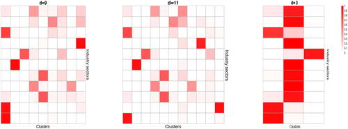
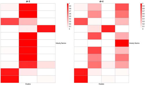
If we take and
and
. The clustering results with
and 3 are presented in is presented in . The first cluster mainly consists of the companies in Consumer Staples, Real Estate and Utilities, Clusters 2 and 3 contain the companies in, respectively, Health Care and Financials, Cluster 4 contains mainly some companies in Communication Service and Information Technology, Cluster 5 consists of the companies in Industrials and Materials, Cluster 6 are mainly the companies in Consumer Discretionary, Cluster 7 is a mixture of a small number of companies from each of 5 or 6 different sectors, Cluster 8 is mainly the companies from Information Technology, Cluster 9 contains almost all companies in Energy. To examine how stable the clustering is, we also include the results for d = 11 and d = 3 in . When d is increased from 9 to 11, the original Cluster 1 is divided into new Clusters 1 and 11 with the former consisting of Consumer Staples and Utilities sectors, and the latter being Real Estate sector. Furthermore the original Cluster 7 splits into new Clusters 7 and 10, while the other 7 original clusters are hardly changed. With d = 3, most companies in each of the 11 sectors stay in one cluster.
Fig. 4 Heat-maps of the distributions of the stocks in each of the 11 industry sectors (corresponding to 11 rows) over d clusters (corresponding to d columns), with and 3. The estimated numbers of the common and cluster-specific factors are, respectively,
and
.
If we take and
, the estimated
is unchanged. The clustering results with
and 3 are presented in . Comparing with , there are some striking similarities: First the clustering with d = 3 are almost identical. For d = 9, the profiles of Clusters 2, …, 6, 8, and 9 are not significantly changed while Clusters 1 and 7 in are somehow mixed together in . With d = 11, the profiles of Clusters 2 – 6, 8 – 10 in the two figures are about the same while Clusters 7 and 11 are mixed up across the two figures.
Fig. 5 Heat-maps of the distributions of the stocks in each of the 11 industry sectors (corresponding to 11 rows) over d clusters (corresponding to d columns), with and 3. The estimated numbers of the common and cluster-specific factors are, respectively,
and
.
The analysis above indicates that the companies in the same industry sector tend to share similar dynamic structure in the sense that they are driven by the same cluster-specific factors. Our analysis is reasonably stable as most the clusters do not change substantially when the number of the weaker factors chooses different values , or
.
We also apply method of Ando and Bai (Citation2017) to this dataset; leading to the same estimate , but smaller estimates
and
. The clustering results for
and
are presented in which similar to the right parts in , though the method of Ando and Bai (Citation2017) puts energy companies as a separate group. In contrast, our method puts financial companies as a separate group. Note that classical papers in Finance (e.g., Berger and Ofek, Citation1995; Denis, Denis, and Yost, Citation2002; Lemmon, Roberts, and Zender, Citation2008) often eliminate financial companies from other companies.
Fig. 6 Heat-maps of the distributions of the stocks in each of the 11 industry sectors (corresponding to 11 rows) over d clusters (corresponding to d columns) based on Ando and Bai (Citation2017).
7 Miscellaneous Comments
Robustness
We identify and distinguish common factors and cluster-specific factors by the different factor strengths, that is, common factors are strong with δ = 0, and cluster-specific factors are weak with . However if, for example, one of the common factors has the same strength as the cluster-specific factors, the number of the strong factor is then
and the number of the weak factors is r + 1. In this case, the estimated
and the factor loading spaces will all be wrong. Nevertheless a common factor has nonzero loadings on the most components of
, hence, those loadings must be extremely small in order to be a weak factor. Therefore, its impact on the estimation of the number of clusters, and the misclassification rates is minor. Simulation results in supplementary materials support this assertion.
Heterogeneous factor strength
We assume two factor strengths: p for common factors and for cluster-specific factors. If there are s different strengths
among the cluster-specific factors, we can search for the s largest local maximums among
in Step 1. Moreover, Step 2 should be repeated s times to estimate s factor loadings corresponding to different factor strengths. While the asymptotic results can be extended accordingly, small values such as
are sufficient for most practical applications.
Estimation for rj and
When we cluster the time series correctly in Steps 4–5, we obtain the estimator for from
directly. We can also run Step 1 on each cluster to estimate rj. Theorem 3 ensures the consistency of those estimates. Although Theorem 7 ensures that most of time series can be clustered correctly, there may be a cluster obtained in Step 5 which is not accuracy enough. It remains an open problem to evaluate how the clustering error is propagated into the estimation for rj and
.
Supplementary Materials
All the technical proofs are presented in an online supplementary which also contains additional simulation results. We also provide the dataset and codes in Section 6 in an online supplementary.
Supplemental Material
Download Zip (2.9 MB)Acknowledgments
We would like to thank three reviewers, the associate editor and the editor for their comments and suggestions. We would like to thank Professor Tomohiro Ando and Professor Jushan Bai for kindly providing us with the computer code for the simulations in Ando and Bai (Citation2017).
Disclosure Statement
There are no relevant competing interests to declare.
Additional information
Funding
Related Research Data
References
- Aghabozorgi, S., Shirkhorshid, A. S., and Wah, T. Y. (2015), “Time-Series Clustering – A Decade Review,” Information System, 53, 16–38. DOI: 10.1016/j.is.2015.04.007.
- Alonso, A. S., and Peña, D. (2019), “Clustering Time Series by Linear Dependency,” Statistics and Computing, 29, 655–676. DOI: 10.1007/s11222-018-9830-6.
- Ando, T., and Bai, J. (2017), “Clustering Huge Number of Financial Time Series: A Panel Data Approach with High-Dimensional Predictors and Factor Structures,” Journal of the American Statistical Association, 519, 1182–1198. DOI: 10.1080/01621459.2016.1195743.
- Berger, P. G., and Ofek, E. (1995), “Diversification’s Effect on Firm Value,” Journal of Financial Economics, 37), 39–65. DOI: 10.1016/0304-405X(94)00798-6.
- Chamberlain, G. (1983), “Funds, Factors, and Diversification in Arbitrage Pricing Models,” Econometrica, 51, 1305–1323. DOI: 10.2307/1912276.
- Chamberlain, G., and Rothschild, M. (1983), “Arbitrage, Factor Structure, and Mean-Variance Analysis on Large Asset Markets,” Econometrica, 51, 1281–1304. DOI: 10.2307/1912275.
- Chang, J., Gao, B., and Yao, Q. (2015), “High Dimensional Stochastic Regression with Latent Factors, Endogeneity and Nonlinearity,” Journal of Econometrics, 189, 297–312. DOI: 10.1016/j.jeconom.2015.03.024.
- Denis, D. J., Denis, D. K., and Yost, K. (2002), “Global Diversification, Industrial Diversification, and Firm Value,” Journal of Finance, 57, 1951–1979. DOI: 10.1111/0022-1082.00485.
- Esling, P., and Agon, C. (2012), “Time-Series Data Mining,” ACM Computing Survey, 45, Article 12. DOI: 10.1145/2379776.2379788.
- Frühwirth-Schnatter, S., and Kaufmann, S. (2008), “Model-based Clustering of Multiple Time Series,” Journal of Business & Economic Statistics, 26, 78–89. DOI: 10.1198/073500107000000106.
- Kakizawa, Y., Shumway, R. H., and Taniguchi, M. (1998), “Discrimination and Clustering for Multivariate Time Series,” Journal of the American Statistical Association, 93, 328–340. DOI: 10.1080/01621459.1998.10474114.
- Keogh, E., and Lin, J. (2005), “Clustering of Time-Series Subsequences is Meaningless: Implications for Previous and Future Research,” Knowledge and Information Systems, 8, 154–177. DOI: 10.1007/s10115-004-0172-7.
- Keogh, E., and Ratanamahatana, C. A. (2005), “Exact Indexing of Dynamic Time Warping,” Knowledge and Information Systems, 7, 358–386. DOI: 10.1007/s10115-004-0154-9.
- Khaleghi, A., Ryabko, D., Mary, J., and Preux, P. (2016), “Consistent Algorithms for Clustering Time Series,” Journal of Machine Learning Research, 17, 1–32.
- Lam, C., and Yao, Q. (2012), “Factor Modelling for High-Dimensional Time Series: Inference for the Number of Factors,” The Annals of Statistics, 40, 694–726. DOI: 10.1214/12-AOS970.
- Lemmon, M. L., Roberts, M. R., and Zender, J. F. (2008), “Back to the Beginning: Persistence and the Cross-Section of Corporate Capital Structure,” Journal of Finance, 63, 1575–1608. DOI: 10.1111/j.1540-6261.2008.01369.x.
- Li, Z., Wang, Q., and Yao, J. (2017), “Identifying the Number of Factors from Singular Values of a Large Sample Auto-Covariance Matrix,” The Annals of Statistics, 45, 257–288. DOI: 10.1214/16-AOS1452.
- Liao, T. W. (2005), “Clustering of Time Series Data – A Survey,” Pattern Recognition, 38, 1857–1874.
- Maharaj, E. A., D’Urso, P., and Caiado, J. (2019), Time Series Clustering and Classification, Boca Raton, FL: Chapman and Hall/CRC.
- Roelofsen, P. (2018), “Time Series Clustering,” Vrije Universiteit Ansterdam. Available at https://www.math.vu.nl//ensuremath{/sim}sbhulai/papers/thesis-roelofsen.pdf.
- Yao, Q., Tong, H., Finkenstädt, B., and Stenseth, N. C. (2000), “Common Structure in Panels of Short Ecological Time Series,” Proceeding of the Royal Society (London), B, 267, 2457–2467.
- Zhang, T. (2013), “Clustering High-Dimensional Time Series based on Parallelism,” Journal of the American Statistical Association, 108, 577–588. DOI: 10.1080/01621459.2012.760458.
- Zolhavarieh, S., Aghabozorgi, S., and Teh, Y. W. (2014), “A Review of Subsequence Time Series Clustering,” The Scientific World Journal, 2014, 312512. DOI: 10.1155/2014/312521.