Semiparametric Proximal Causal Inference

Abstract

Skepticism about the assumption of no unmeasured confounding, also known as exchangeability, is often warranted in making causal inferences from observational data; because exchangeability hinges on an investigator’s ability to accurately measure covariates that capture all potential sources of confounding. In practice, the most one can hope for is that covariate measurements are at best proxies of the true underlying confounding mechanism operating in a given observational study. In this article, we consider the framework of proximal causal inference introduced by Miao, Geng, and Tchetgen Tchetgen and Tchetgen Tchetgen et al. which while explicitly acknowledging covariate measurements as imperfect proxies of confounding mechanisms, offers an opportunity to learn about causal effects in settings where exchangeability on the basis of measured covariates fails. We make a number of contributions to proximal inference including (i) an alternative set of conditions for nonparametric proximal identification of the average treatment effect; (ii) general semiparametric theory for proximal estimation of the average treatment effect including efficiency bounds for key semiparametric models of interest; (iii) a characterization of proximal doubly robust and locally efficient estimators of the average treatment effect. Moreover, we provide analogous identification and efficiency results for the average treatment effect on the treated. Our approach is illustrated via simulation studies and a data application on evaluating the effectiveness of right heart catheterization in the intensive care unit of critically ill patients. Supplementary materials for this article are available online.

Keywords:

• Double robustness
• Efficient influence function
• Identification
• Proximal causal inference
• Semiparametric theory
• Unmeasured confounding

1 Introduction

A common assumption for causal inference from observational data is that of no unmeasured confounding, which states that one has measured a sufficiently rich set of covariates to ensure that within covariate strata, subjects are exchangeable across observed treatment values. Skepticism about such exchangeability assumption in observational studies is often warranted because it essentially requires investigators to accurately measure covariates capturing all potential sources of confounding. In practice, confounding mechanisms can rarely be learned with certainty from measured covariates. One may therefore only hope that covariate measurements are at best proxies of true underlying confounders.

There is a growing literature on formal causal inference methods that leverage certain types of proxies known as negative control variables to mitigate confounding bias in analysis of observational data (Lipsitch, Tchetgen, and Cohen 2010; Kuroki and Pearl 2014; Miao, Geng, and Tchetgen Tchetgen 2018; Shi et al. 2019; Shi, Miao, and Tchetgen Tchetgen 2020). Existing negative control methods rely for point identification of causal effects on fairly restrictive assumptions such as linear models for the outcome and the unmeasured confounder (Flanders et al. 2011; Gagnon-Bartsch and Speed 2012; Flanders, Strickland, and Klein 2015; Wang et al. 2017), rank preservation (Tchetgen Tchetgen 2014), monotonicity (Sofer et al. 2016), or categorical unmeasured confounders (Shi et al. 2019). Miao, Geng, and Tchetgen Tchetgen (2018) stands out in this literature as they formally establish sufficient conditions for nonparametric identification of causal effects using a pair of treatment and outcome proxies in the point treatment setting.

Building on Miao, Geng, and Tchetgen Tchetgen (2018), Tchetgen Tchetgen et al. (2020) recently introduced a potential outcome framework for proximal causal inference, which offers an opportunity to learn about causal effects in point treatment and time-varying treatment settings where exchangeability on the basis of measured covariates fails. Proximal causal inference essentially requires that the analyst can correctly classify a subset of measured covariates into three bucket types: (1) variables that may be common causes of the treatment and outcome variables; (2) treatment-inducing confounding proxies versus; (3) outcome-inducing confounding proxies. A proxy of type (2) is a potential cause of the treatment which is related with the outcome only through an unmeasured common cause for which the variable is a proxy; while a proxy of type (3) is a potential cause of the outcome which is related with the treatment only through an unmeasured common cause for which the variable is a proxy. Proxies that are associated with an unmeasured confounder but that are neither causes of treatment or outcome variables can belong to either bucket type (2) or (3).

Examples of proxies of type (2) and (3) abound in observational studies. For instance, in an observational study evaluating the effects of a treatment on disease progression, one is typically concerned that patients either self-select or are selected by their physician to take the treatment based on prognostic factors for the outcome; therefore, there may be two distinct processes contributing to a subject’s propensity to be treated. In an effort to account for these sources of confounding, a diligent investigator would endeavor to record biomarker lab measurements and other clinically relevant covariate data. Lab measurements of biomarkers are well-known to be error prone and therefore to at best serve as proxies of patients’ underlying biological mechanisms at the source of confounding. Even when such measurements are available to the physician for treatment decision making, they seldom constitute a cause of disease progression (e.g., CD4 count or viral load in HIV care), but may be strongly associated with the latter to the extent that they share an unmeasured common cause (e.g., CD4 count is a proxy of underlying immune system status), and therefore may be viewed as proxies of type (2). As discussed in Shi, Miao, and Tchetgen Tchetgen (2020), pretreatment variables that satisfy the three core instrumental variable (IV) conditions (IV relevance, IV independence and exclusion restriction) constitute valid proxies of type (2); and in fact remain valid proxies even if IV independence assumption is violated (Shi, Miao, and Tchetgen Tchetgen 2020). A prominent proxy of type (3) often entails a baseline measurement of the outcome process, the basis of which serves as justification of the widely used difference-in-differences approach to account for confounding bias under no interaction assumptions or monotonicity conditions (Sofer et al. 2016). Lifestyle choices such as exercising, alcohol use, smoking behavior, nutritional habits, and other measurements of health seeking behaviors or self-reported health status are routinely collected via questionnaires with the implicit understanding that although such measurements are often well-validated instruments, they should be viewed as proxies of the latent factors inducing confounding in causal queries about potential public health or public policy interventions on health and related outcomes. Extensive discussion of proxies encountered in health and social sciences can be found in Lipsitch, Tchetgen, and Cohen (2010), Kuroki and Pearl (2014), Miao, Geng, and Tchetgen Tchetgen (2018), Sofer et al. (2016), Shi et al. (2019), Shi, Miao, and Tchetgen Tchetgen (2020); the proposed proximal causal inference framework is therefore a unifying framework for identification and inference leveraging the various types of proxies that have appeared in prior literature.

Other prominent examples of treatment and outcome proxies are negative control treatment and outcome variables routinely used in recent literature on the protective effectiveness of COVID-19 vaccination in real world settings (Patel, Jackson, and Ferdinands 2020; Dagan et al. 2021; Thompson et al. 2021; Olson et al. 2022; Li et al. in press). For example, in Li et al. (in press), immunization visits before December 2020, when the COVID-19 vaccine became available, were used as treatment confounding proxies and the following diagnoses after April 5, 2021 were used as outcome confounding proxies: arm/leg cellulitis, eye/ear disorder, gastroesophageal disease, atopic dermatitis, and injuries. Aside for these proxies, there may also be factors that can accurately be described as true common causes of treatment and outcome processes; these variables collected in bucket type (1) may in fact include age, gender, race or ethnicity, and years of education depending on the context. Thus, rather than assuming that exchangeability can be attained by adjusting for measured covariates, our proposed proximal framework requires that the investigator can correctly select proxies of types (2) and (3) relative to a latent factor (possibly multivariate) that would in principle suffice to account for confounding; this condition is formalized using the potential outcomes framework in the following section. In terms of proximal estimation and inference, Tchetgen Tchetgen et al. (2020) focus primarily on so-called proximal g-computation, a generalization of Robins’ g-computation algorithm which may be viewed essentially as maximum likelihood estimation, requiring a correctly specified model for the entire data generating mechanism; in case of linear models, they proposed a proximal recursive two-stage least squares algorithm for point and time-varying treatments which is somewhat more robust provided the specified linear models are correct.

In this article, we develop a general semiparametric framework for proximal causal inference about the population average treatment effect (ATE) and the average treatment effect on the treated (ATT) using proxies of types (2) and (3) while accounting for a possibly large number of observed covariates in the point treatment setting. In addition, we establish an alternative condition to that of Miao, Geng, and Tchetgen Tchetgen (2018), Shi et al. (2019), and Tchetgen Tchetgen et al. (2020) for nonparametric proximal identification of the average treatment effect in case of a point intervention; and we subsequently characterize the semiparametric efficiency bound for the identifying functional of the ATE under two key semiparametric models that place different restrictions on the observed data distribution, as well as under a nonparametric model in which both sets of restrictions are relaxed. We then propose a class of doubly robust locally efficient estimators of the average treatment effect that are consistent provided one of two aforementioned models restricting the observed data distribution is correct, but not necessarily both. The proposed estimators are locally efficient in the sense that when all working models are correctly specified (i.e., the intersection submodel), our estimators achieve the semiparametric efficiency bound for estimating the average treatment effect under the union model. Analogous results are obtained for the ATT in the Appendix G, supplementary materials.

The remainder of the article is organized as followed. In Section 2, we briefly review proximal identification results of ATE (Miao, Geng, and Tchetgen Tchetgen 2018; Shi et al. 2019; Tchetgen Tchetgen et al. 2020) before introducing an alternative condition for nonparametric identification of ATE (and ATT). In Section 3, we develop semiparametric theory for proximal causal inference (Tchetgen Tchetgen et al. 2020) and describe construction of doubly robust and semiparametric locally efficient estimators. In Section 4, we draw parallels between the proposed doubly robust proximal estimators and standard augmented inverse-probability-weighted estimators developed by Robins and colleagues under no unmeasured confounding (Scharfstein, Rotnitzky, and Robins 1999); we establish that the former may be viewed as a generalization of the latter allowing for unmeasured confounding under our identifying assumptions. Simulation studies are presented in Section 5. Section 6 describes a real data application on evaluating the effectiveness of right heart catheterization in the intensive care unit of critically ill patients. The article concludes with a discussion of future work in Section 7. Proofs and additional results are provided in the Appendix, supplementary materials.

2 Nonparametric Proximal Identification of the Average Treatment Effect

2.1 Background

We consider estimating the effect of a binary treatment A on an outcome Y subject to potential unmeasured confounding. Throughout, we let U denote the unmeasured confounder (possibly vector-valued) which may be discrete, or continuous, or include both types of variables. Let $Y(a)$, $a=0,1$ denote the potential outcome that would be observed if the treatment were set to a. We are interested in the population average treatment effect defined as $\psi =\mathbb{E}[Y(1)-Y(0)]$. We assume that the following consistency assumption holds:

Assumption 1

(Consistency).

$Y=Y(A)$ almost surely.

Moreover, suppose that one has measured covariates L such that:

Assumption 2

(Positivity).

$0<\mathrm{Pr}(A=a|L)<1$ almost surely, $a=0,1$.

A common identification strategy in observational studies invokes exchangeability condition on the basis of measured covariates.

Assumption 3

(Exchangeability).

$Y(a)\perp A|L$ for $a=0,1$.

Assumption 3 is sometimes interpreted as stating that L includes all common causes of A and Y; an assumption represented in causal directed acyclic graph (DAG) in Figure 1(a), in which case L is of type (1). Under Assumptions 1–3, it is known that the counterfactual mean $\mathbb{E}[Y(a)]$ is identified by celebrated g-formula (Robins 1986; Hernán and Robins 2020).

Figure 1: DAGs representing treatment and outcome confounding proxies when exchangeability holds.

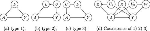
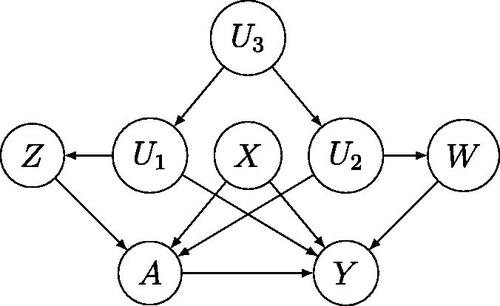
It is also interesting to consider alternative data generating mechanisms under which Assumption 3 holds, illustrated in Figures 1(b) and (c), with the first of type (2) where L includes all causes of A that share an unmeasured common cause U (and therefore are associated) with Y; while the second is of type (3) where L includes all causes of Y that share an unmeasured common cause U (and therefore are associated) with A. Measured covariates of types (1), (2), and (3) may coexist, as depicted in Figure 1(d), in which case L has been decomposed into three bucket types of measured covariates $L=(X,W,Z),$ such that X are measured covariates of type (1), Z are measured covariates of type (2), and W are measured covariates of type (3). All four settings represented in Figure 1 illustrate possible data generating mechanisms under which exchangeability Assumption 3 holds, without necessarily requiring that the analyst identify which bucket type each covariate in L belongs to. Note that all four settings rule out the presence of an unmeasured common cause of A and Y, therefore ruling out unmeasured confounding.

In order for exchangeability to hold in Figure 1(d), it must be that as encoded in the DAG, unmeasured variables $U_1$ and $U_2$ are independent conditional on A, X, Z, and W; otherwise, as illustrated in Figure 2, the unblocked backdoor path $A-U_2-U_3-U_1-Y$ would invalidate Assumption 3. As shown in the next section, it is possible to relax this conditional independence assumption and therefore Assumption 3 while preserving identification of the counterfactual mean parameter despite the presence of unmeasured confounding.

Figure 2: Coexistence of types (1), (2), and (3) proxies when exchangeability fails.

2.2 Proximal Identification

Now consider a setting in which exchangeability Assumption 3 fails. Suppose that one has partitioned L into variables $(X,Z,W)$, such that Z includes treatment-inducing confounding proxies, and W includes outcome-inducing confounding proxies known to satisfy the following Assumptions 4–6 which formalize the notion of covariate types (2) and (3).

Assumption 4

(Conditional independence for Y). $$Y\perp Z|U,X,A.$$

Assumption 5

(Conditional independence for W). $$W\perp (Z,A)|U,X.$$

Assumption 6

(Conditional randomization). $$Y(a)\perp A|U,X \text{for} a=0,1.$$

Figure 3 provides a graphical representation of Assumptions 4–6. For instance, Assumptions 4 and 5 formalize the hypothesis in Li et al. (in press) discussed in Section 1 that prior immunization visits are valid treatment confounding proxies and diagnoses such as arm/leg cellulitis, eye/ear disorder, injuries are valid outcome confounding proxies. As discussed in Shi, Miao, and Tchetgen Tchetgen (2020), a number of alternative DAGs are in fact compatible with Assumptions 4–6; see Table A.1 of Tchetgen Tchetgen et al. (2020) and Shi, Miao, and Tchetgen Tchetgen (2020). In addition, we make the following positivity assumption for nonparametric identification.

Figure 3: A causal DAG of proximal causal inference.

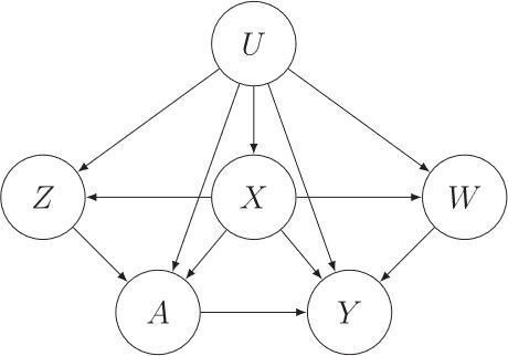
Table 1: Simulation results: absolute bias ($\times {10}^{-2}$) and MSE ($\times {10}^{-2}$).

		${\widehat{\psi }}_{\text{DR}}$	${\widehat{\psi }}_{\text{POR}}$	${\widehat{\psi }}_{\text{PIPW}}$	${\widehat{\psi }}_{\text{PDR}}$
Scenario 1	Bias	9.9	0.4	0.5	0.5
	MSE	1.1	0.6	0.7	0.7
Scenario 2	Bias	23.4	64.0	0.5	0.1
	MSE	6.5	47.5	0.7	3.0
Scenario 3	Bias	17.3	0.4	20.4	0.2
	MSE	3.2	0.6	4.5	0.7
Scenario 4	Bias	43.2	30.0	13.7	34.5
	MSE	19.9	19.2	2.3	23.5

${\widehat{\psi }}_{\text{DR}}$ refers to the standard doubly robust estimator; ${\widehat{\psi }}_{\text{POR}}$ refers to the proximal outcome regression approach; ${\widehat{\psi }}_{\text{PIPW}}$ refers to the proximal treatment confounding bridge approach; ${\widehat{\psi }}_{\text{PDR}}$ refers to the proximal doubly robust estimator.

Assumption 7

(Positivity).

$0<\mathrm{Pr}(A=a|U,X)<1$ almost surely, $a=0,1$.

Assumption 7 essentially states that the probability of having a particular level of exposure, conditional on X and U, is greater than zero for all strata. In order to identify the population average treatment effect, Miao, Geng, and Tchetgen Tchetgen (2018), and Tchetgen Tchetgen et al. (2020) consider the following assumptions:

Assumption 8

(Completeness).

For any square-integrable function g and for any a, x, $\mathbb{E}[g(U)|Z,A=a,X=x]=0$ almost surely if and only if $g(U)=0$ almost surely.

These conditions are formally known as completeness conditions which can accommodate both categorical and continuous confounders. Completeness is a technical condition central to the study of sufficiency in foundational theory of statistical inference. We note that the completeness Assumption 8 rules out conditional independence of U and Z given A and X. Here one may interpret the completeness condition as a requirement relating the range of U to that of Z which essentially states that the set of proxies must have sufficient variability relative to variability of U. The condition is easiest understood in the case of categorical U and Z with number of categories $d_u$ and $d_z$, respectively. In this case, completeness Assumption 8 requires that (1) $$d_z\ge d_u,$$(1) which states that Z must have at least as many categories as U. Intuitively, condition (1) states that proximal causal inference can potentially account for unmeasured confounding in the categorical case as long as the number of categories of U is no larger than that of Z (Miao, Geng, and Tchetgen Tchetgen 2018; Shi et al. 2019; Tchetgen Tchetgen et al. 2020). This further provides a rationale for measuring a rich set of baseline characteristics in observational studies as a potential strategy for mitigating unmeasured confounding via the proximal approach we describe below. Many commonly used parametric and semiparametric models such as exponential families (Newey and Powell 2003) satisfy the completeness condition. For nonparametric regression models, results of D’Haultfoeuille (2011) and Darolles et al. (2011) can be used to justify the completeness condition, although they focused on nonparametric instrumental variable problems where completeness also plays an important role. Chen et al. (2014) and Andrews (2017) showed that if Z and U are continuously distributed and the dimension of Z is larger than that of U, then under a mild regularity condition, the completeness condition holds generically in the sense that the set of distributions for which completeness fails has a property similar to being essentially Lebesgue measure zero. More specifically, as formally shown by Canay, Santos, and Shaikh (2013), distributions for which a completeness condition fails can approximate distributions for which it holds arbitrarily well in the total variation distance sense. Thus, while completeness conditions may themselves not be directly testable, one may argue as in Canay, Santos, and Shaikh (2013) that they are commonly satisfied. We further refer to Chen et al. (2014), Andrews (2017), and Section 2 of the supplementary material of Miao et al. (2022) for a review and examples of completeness.

Miao, Geng, and Tchetgen Tchetgen (2018) established the following nonparametric identification result which we have adapted to the proximal inference setting.

Theorem 2.1.

(Miao, Geng, and Tchetgen Tchetgen 2018) Suppose that there exists an outcome confounding bridge function $h(w,a,x)$ that solves the following integral equation (2) $$\mathbb{E}\left[Y\right|Z,A,X]=\int h(w,A,X)dF(w|Z,A,X),$$(2) almost surely.

1. (Factuals) Under Assumptions 4, 5, 7, and 8, one has that (3) $$\mathbb{E}\left[Y\right|U,A,X]=\int h(w,A,X)dF(w|U,X),$$(3) almost surely.

2. (Causal) Suppose that (3) holds. Under Assumptions 1, 6, and 7, the counterfactual mean $\mathbb{E}[Y(a)]$ is nonparametrically identified by (4) $$\mathbb{E}[Y(a)]={\int }_{\mathcal{X}}\int h(w,a,x)dF(w|x)dF(x),$$(4) and thus the average treatment effect is identified by $$\psi =\int {}_{\mathcal{X}}\int [h(w,1,x)-h(w,0,x)]dF(w|x)dF(x).$$

Remark 1.

Technical conditions for the existence of a solution to (2) are provided in the Appendix B, supplementary materials. In particular, we note that the following assumption:

Assumption 9

(Completeness).

For any square-integrable function g and for any a, x, $\mathbb{E}[g(Z)|W,A=a,X=x]=0$ almost surely if and only if $g(Z)=0$ almost surely.along with the regularity conditions on the singular value decomposition of the conditional mean operators together, suffice for the existence of a solution to (2).

Theorem 2.1 serves as a basis for inference in Shi et al. (2019), Tchetgen Tchetgen et al. (2020), Miao and Tchetgen Tchetgen (2018), as described in Section 3. Equation (2)(2) $$\mathbb{E}\left[Y\right|Z,A,X]=\int h(w,A,X)dF(w|Z,A,X),$$(2) defines a so-called inverse problem known as a Fredholm integral equation of the first kind (Kress 1989; Miao, Geng, and Tchetgen Tchetgen 2018). Importantly, while the theorem does not require uniqueness of a solution to the integral (2), all solutions lead to a unique value of the ATE. Note that (3) highlights the inverse problem nature of the task accomplished by (4) (Tchetgen Tchetgen et al. (2020) refer to (4) as proximal g-formula), which is to determine a function h that satisfies this equality without explicitly modeling or estimating the latent factor U. A remarkable feature of proximal causal inference is that accounting for U without either measuring U directly or estimating its distribution can be accomplished provided that the set of proxies though imperfect, is sufficiently rich so that the inverse problem admits a solution.

Remark 2.

There are different strategies to achieve identification in proximal causal inference. Instead of taking (2) as a starting point, Miao and Tchetgen Tchetgen (2018) consider an alternative identifying condition in which they assume that there exists a bridge function $h^{\prime }(w,a,x)$ such that $\mathbb{E}[Y|U,a,X]=\int h^{\prime }(w,a,X)dF(w|U,X)$ almost surely. In addition, Miao and Tchetgen Tchetgen (2018) replace completeness Assumption 8 which involves unobservables with an alternative completeness condition that only involves observables; that is, for any square-integrable function g and for any a, x, $\mathbb{E}[g(W)|Z,a,x]=0$ almost surely if and only if $g(W)=0$ almost surely. They then establish that such function $h^{\prime }$ must solve (2), and arrive at the very same identifying proximal g-formula (4).

2.3 A New Proximal Identification Result

In this section, we establish an alternative proximal identification result to that of Miao, Geng, and Tchetgen Tchetgen (2018). We first consider identification with a discrete variable U. Suppose that W, Z, U are discrete variables, each with d categories. For notational convenience, we write $P(Z|w)={(\mathrm{Pr}(z_1|w),\dots ,\mathrm{Pr}(z_d|w))}^T$, $P(z|W)=(\mathrm{Pr}(z|w_1),\dots ,\mathrm{Pr}(z|w_d))$, and $P(Z|W)=(\mathrm{Pr}(Z|w_1),\dots ,\mathrm{Pr}(Z|w_d))$ to denote a column vector, a row vector, and a matrix, respectively. For other variables, vectors and matrices are analogously defined. By $(Z,A)\perp W|U,X$, we have that $$\begin{array}{cc}P(Z|W,a,x)=P(Z|U,a,x)P(U|W,a,x),\hfill & \hfill \\ P{(a|W,x)}^{-1}=P{(a|U,x)}^{-1}P(U|W,a,x),\hfill & \hfill \end{array}$$where $P{(a|W,x)}^{-1}$ denotes $(1/\mathrm{Pr}(a|w_1,x),\dots ,1/\mathrm{Pr}(a|w_d,x))$ and $P{(a|U,x)}^{-1}$ denotes $(1/\mathrm{Pr}(a|u_1,x),\dots ,1/\mathrm{Pr}(a|u_d,x))$. Therefore, assuming that $P(Z|W,a,X)$ is invertible for any $a=0,1$ and x, we have that $$\begin{array}{cc}P{(a|W,x)}^{-1}{P}^{-1}(Z|W,a,x)P(Z|U,a,x)\hfill & =P{(a|U,x)}^{-1},\hfill \end{array}$$ where $P^{-1}(Z|W,a,x)$ denotes the inverse of the matrix $P(Z|W,a,x)$. Furthermore, by $Y\perp Z|U,A,X$, $$\begin{array}{cc}P(y|U,a,x)=[P{(a|W,x)}^{-1}{P}^{-1}(Z|W,a,x)P(Z|U,a,x)]\hfill & \hfill \\ \times P(a|U,x)\times P(y|U,a,x)\hfill & \hfill \\ =P{(a|W,x)}^{-1}{P}^{-1}(Z|W,a,x)P(y,a,Z|U,x),\hfill & \hfill \end{array}$$ where $\times$ denotes element-wise multiplication. Upon multiplying both sides by ${(\mathrm{Pr}(u_1|x),\dots ,\mathrm{Pr}(u_d|x))}^T$, we have that $$\mathrm{Pr}(y(a)|x)=P{(a|W,x)}^{-1}{P}^{-1}(Z|W,a,x)P(y,a,Z|x).$$

Therefore, establishing identification of $\mathrm{Pr}(y(a)|x)$, and thus, identification of corresponding functionals, such as counterfactual means and average treatment effect. Next, we extend this identification result to a general setting in which U can include both categorical and continuous factors, under the following completeness condition.

Assumption 10

(Completeness).

For any square-integrable function g and for any a, x, $\mathbb{E}[g(U)|W,A=a,X=x]=0$ almost surely if and only if $g(U)=0$ almost surely.

Assumption 10 essentially states that W must have sufficient variability relative to variability of U.

Theorem 2.2.

Suppose that there exists a treatment confounding bridge function $q(z,a,x)$ that solves the integral equation: (5) $$\mathbb{E}[q(Z,a,X)|W,A=a,X]=\frac{1}{f(A=a|W,X)},$$(5) almost surely.

1. (Factuals) Under Assumptions 5, 7, and 10, one has that (6) $$\int q(z,a,X)dF(z|U,A=a,X)=\frac{1}{f(A=a|U,X)},$$(6) almost surely. Furthermore, if Assumption 4 also holds, one also has that (7) $$\mathbb{E}\left[Y\right|U,A=a,X=x]=\mathbb{E}[I(A=a)Yq(Z,a,X)|U,X=x],$$(7) almost surely.

2. (Causal) Suppose that (7) holds. Under Assumptions 1, 6, and 7, $\mathbb{E}[Y(a)]$ is nonparametrically identified by (8) $$\mathbb{E}[Y(a)]={\int }_{\mathcal{X}}\int I(\tilde{a}=a)q(z,a,x)\mathit{ydF}(y,z,\tilde{a}|x)dF(x).$$(8) Therefore, the average treatment effect is identified by $$\psi ={\int }_{\mathcal{X}}\int {(-1)}^{1-a}q(z,a,x)\mathit{ydF}(y,z,a|x)dF(x).$$

Remark 3.

We note that Theorem 2.2 also applies for a continuous possibly multivariate exposure A with $$\mathbb{E}[Y(a)]={\int }_{\mathcal{X}}{\int }_{\mathcal{Y},\mathcal{Z}}q(z,a,x)\mathit{ydF}(y,z,a|x)dF(x).$$

Remark 4.

Formal technical conditions for the existence of a solution to (5) are provided in the Appendix B, supplementary materials. In particular, we note that the following assumption:

Assumption 11

(Completeness).

For any square-integrable function g and for any a, x, $\mathbb{E}[g(W)|Z,A=a,X=x]=0$ almost surely if and only if $g(W)=0$ almost surely.along with the regularity conditions on the singular value decomposition of the conditional mean operators together, suffice for the existence of a solution to (5).

Theorem 2.2 provides a new proximal identification result which complements that of Miao, Geng, and Tchetgen Tchetgen (2018) and Tchetgen Tchetgen et al. (2020). Similar to (2) and (5) also defines a Fredholm integral equation of the first kind. Fredholm equations are well known to often be ill-posed and solving them requires a form of regularization in practice. In the next section, we will consider using semiparametric models as an implicit form of regularization. We note that exchangeability assumption, albeit a structural assumption, can also be viewed as a form of regularization of (2) and (5) which automatically yields unique and stable solutions to the integral equations. Intuitively, suppose that $U=\varnothing$, then (2) reduces to $$\mathbb{E}\left[Y\right|A,X]=\int \mathbb{E}(Y|w,A,X)dF(w|A,X),$$that is, $h(w,a,x)=\mathbb{E}(Y|w,a,x)$; alternatively, suppose that $U=\varnothing$, then (5) reduces to $$\frac{1}{f(A=a|X)}=\int \frac{1}{f(A=a|z,X)}dF(z|A=a,X),$$ that is, $q(z,a,x)=1/f(A=a|z,x)$.

Note that again (6) highlights the inverse problem nature of the task accomplished by (8), which is to determine a function q that satisfies the equation without explicitly modeling or estimating the latent factor U. The theorem reveals that accounting for U without either measuring U directly or estimating its distribution can be accomplished provided that the set of proxies is sufficiently rich so that the inverse problem admits a solution.

Remark 5.

Note that similar to Remark 2, instead of assuming (5), one could alternatively consider the following identifying condition: suppose that there exists a bridge function $q^{\prime }(z,a,x)$ such that $1/f(A=a|U,X)=\int q^{\prime }(z,a,X)dF(z|U,A=a,X)$ almost surely, and replace completeness Assumption 10 with: for any square-integrable function g and for any a, x, $\mathbb{E}[g(Z)|W,a,x]=0$ almost surely if and only if $g(Z)=0$ almost surely; subsequently by Theorem C.1 presented in the Appendix C, supplementary materials, any solution $q^{\prime }$ must also solve (5); furthermore identifying formula (8) still applies.

Remark 6.

Identification of q under the conditions of Theorem 2.2 offers an opportunity for identification of any smooth functional $\beta$ of the marginal counterfactual distribution that can be defined as a solution to a moment equation, say $\mathbb{E}(\int m(Y(a),a,X;\beta )d\mu (a))=0$, with $\mu$ a dominating measure of a. The theorem implies the following observed data moment equation analog obtained by reweighting the moment equation by the treatment confounding bridge function, that is, $\mathbb{E}(q(Z,A,X)m(Y,A,X;\beta ))=0$, provided that the expectation is well defined. For instance, the marginal distribution of $Y(a)$ at y can be identified by $m(Y(a),a,x;y,\beta )=I(Y(a)\le y)-\beta$. Therefore, identification Theorem 2.2 is more general than Theorem 2.1 which only identifies the ATE.

3 Semiparametric Theory and Inference

We consider inference for $\psi$ under the semiparametric model ${\mathcal{M}}_{sp}$ which places no restriction on the observed data distribution other than existence (but not necessarily uniqueness) of a bridge function h that solves (2). Let $T:L_2(W,A,X)\to L_2(Z,A,X)$ be the conditional expectation operator given by $T(g)\equiv \mathbb{E}[g(W,A,X)|Z,A,X]$, and the adjoint $T^{\prime }:L_2(Z,A,X)\to L_2(W,A,X)$ be $T^{\prime }(g)\equiv \mathbb{E}[g(Z,A,X)|W,A,X]$. We consider the following regularity condition under the model:

Assumption 12.

T and $T^{\prime }$ are surjective.

Theorem 3.1.

We have the following results.

1. Under Assumptions 9 and 11, h and q that solve integral (2) and (5) are uniquely identified.

2. The efficient influence function of $\psi$ under the semiparametric model ${\mathcal{M}}_{sp}$ evaluated at the submodel where Assumption 12 holds, (5) holds at the true data generating law, and h, q are uniquely defined, is given by (9) $$\begin{array}{cc}\mathit{EIF}(\psi )\hfill & ={(-1)}^{1-A}q(Z,A,X)[Y-h(W,A,X)]\hfill \end{array}$$(9) $$+ h(W,1,X)-h(W,0,X)-\psi .$$Therefore, the corresponding semiparametric local efficiency bound of $\psi$ equals $\mathbb{E}[EI{F}^2(\psi )]$.

3. Equation (9)(9) $$\begin{array}{cc}\mathit{EIF}(\psi )\hfill & ={(-1)}^{1-A}q(Z,A,X)[Y-h(W,A,X)]\hfill \end{array}$$(9) admits the double robustness property: $\mathbb{E}[\mathit{EIF}(q^{*},h^{*};\psi )]=0$ provided that either $h^{*}$ is a solution to (2), or $q^{*}$ is a solution to (5), but both do not necessarily hold.

We note that at the submodel where both Assumptions 9 and 11 hold, both completeness of the law of W given Z, $A=a$, $X=x$ and of the law of Z given W, $A=a$, $X=x$ must hold. Therefore, for W and Z finitely valued, this imposes the restriction that the sample space of Z and W have equal cardinality; likewise, for continuous W and Z, this requires that Z and W are of equal dimension. In the event that available candidate proxies W and Z are of unequal dimensions, say W has higher dimension than Z, it may be possible to coarsen W so that its dimension matches the dimension of Z without compromising identification provided Z has higher dimension than U; although a formal approach to operationalize such coarsening is currently lacking in the literature: see Shi et al. (2019) for additional discussion in the categorical unmeasured confounding case. However, we note that formally, the double robustness result of Theorem 3.1(3) does not strictly require either Assumptions 9 or 11 to hold, as uniqueness of either confounding bridge function is not necessary for the efficient influence function to be an unbiased moment equation, only that at least one of the bridge functions satisfies the corresponding integral equation at the true data generating law. For inference, in principle, one may wish for greater robustness to estimate $\psi$ under a nonparametric model for both nuisance functions h and q; this is in fact the approach taken by Ghassami et al. (2022) and Kallus, Mao, and Uehara (2021), who recently adopted the efficient influence function (9) based on an earlier preprint of the current paper, to develop an adversarial inference framework which accommodates reproducing kernel Hilbert space, neural networks and other nonparametric or machine learning estimators of h and q (see also Singh 2020; Mastouri et al. 2021; Kompa et al. 2022 who propose nonparametric methods to evaluate average treatment effect with proximal causal inference). In order for the resulting estimator of the causal effect to be regular, these works require that both nuisance functions can be estimated at rates faster than $n^{-1/4}$ which may not be feasible where L is of moderate to high dimension or depending on the extent to which the integral equations defining either confounding bridge function are ill-posed. It is therefore of interest to develop a doubly robust estimation approach that a priori posits low-dimensional working models for h and q, but however is guaranteed to deliver valid inferences about $\psi$ provided that one but not necessarily both low dimensional models used to estimate h and q can be specified correctly. In this paper, we focus primarily on developing such a doubly robust approach much in the spirit of Scharfstein, Rotnitzky, and Robins (1999), and demonstrate its ability to resolve concerns about ill-posedness and partial model misspecification. In order to describe our proposed doubly robust approach, consider the following two semiparametric models that place parametric restrictions on different components of the observed data likelihood while allowing the rest of the likelihood to remain unrestricted:

${\mathcal{M}}_1$: $h(W,A,X)$ is assumed to be correctly specified and suppose Assumptions 1, 4–8, and 11 hold; ${\mathcal{M}}_2$: $q(Z,A,X)$ is assumed to be correctly specified and suppose Assumptions 1, 4–7, and 9–10 hold.

Our proposed doubly robust locally efficient estimator thus entails modeling both h and q, however, as we will show below only one of these models will ultimately need to be correct for valid inferences about the ATE, without knowing a priori which model is correct. Directly modeling the outcome and treatment confounding bridge functions is a simple and practical regularization strategy that obviates the need to solve complicated integral equations that are well-known to be ill-posed and therefore to admit unstable solutions in practice (Ai and Chen 2003; Newey and Powell 2003; Hall and Horowitz 2005; Horowitz 2011). Illposedness refers to the discontinuity of the operator $T^{-1}$ (or $T^{\prime -1}$), and therefore $T^{-1}\widehat{r}$ (or $T^{\prime -1}\widehat{r}$) might not converge to $T^{-1}r$ (or $T^{\prime -1}r$) under a given norm even if $\widehat{r}$ converges to r with respect to a given norm for r in the range of T (or $T^{\prime }$). In the Appendix E, supplementary materials, we also consider semiparametric efficient inference in submodels ${\mathcal{M}}_1$ and ${\mathcal{M}}_2$, respectively.

Interestingly, the second part of Theorem E.1 in the Appendix E, supplementary materials suggests that, although q solves an integral Equation (5)(5) $$\mathbb{E}[q(Z,a,X)|W,A=a,X]=\frac{1}{f(A=a|W,X)},$$(5) involving the reciprocal of the propensity score function $1/f(A|W,X)$, surprisingly, inferences about a model for q may be obtained without the need for estimating the propensity score provided that an influence function for t is used as an estimating equation. In other words, influence function based estimation of t is fully robust to misspecification of the propensity score as it implicitly uses a nonparametric estimator of the propensity score. The derived influence functions in Theorem E.1 motivate various estimating equations for the corresponding confounding bridge functions $h(W,A,X;b)$ and $q(Z,A,X;t)$, respectively. For instance, if b and t are of dimensions $p_x+p_z+2$ and $p_x+p_w+2$, a natural choice of estimating equations are (10) $${\mathbb{P}}_n\left\{[Y-h(W,A,X;b)]{(1,Z,A,X)}^T\right\}=0,$$(10) (11) $$\begin{array}{c}{\mathbb{P}}_n\{{(-1)}^{1-A}q(Z,A,X;t){(1,W,A,X)}^T\\ \mathrm{\hspace{1em}}\mathrm{\hspace{1em}}- {(0,{(0)}_{p_w},1,{(0)}_{p_x})}^T\}=0,\end{array}$$(11) which correspond to $m(Z,A,X)={(1,Z,A,X)}^T$ and $n(W,A,X)={(-1)}^{1-A}{(1,W,A,X)}^T$ defined in Theorem E.1, where $p_w$ is the dimension of W, $p_z$ is the dimension of Z, $p_x$ is the dimension of X, and the corresponding estimators are denoted by $\widehat{h}$ and $\widehat{q}$, respectively. Linearity in W in h is essentially implied by a proportional relationship between the confounding effects of U on Y and W, although it does not necessarily imply the latter; likewise, linearity in Z in q is implied by (but does not necessarily imply) a logit model between A and U under certain conditions about the distribution of U, for example, Gaussian U. Such estimators can then be used to construct a corresponding substitution estimator of $\psi$. Specifically, proximal outcome regression (POR) and proximal inverse probability weighted (PIPW) estimators are defined as $$\begin{array}{cc}{\widehat{\psi }}_{\text{POR}}={\mathbb{P}}_n\left\{\widehat{h}(W,1,X)-\widehat{h}(W,0,X)\right\},\hfill & \hfill \\ {\widehat{\psi }}_{\text{PIPW}}={\mathbb{P}}_n\left\{{(-1)}^{1-A}\widehat{q}(Z,A,X)Y\right\},\hfill & \hfill \end{array}$$ respectively. Note that as established in the Appendix E, supplementary materials, construction of a locally efficient estimator of h under ${\mathcal{M}}_1$ and q under ${\mathcal{M}}_2$, requires correct specification of additional components of the observed data law beyond q and h. In principle, a locally efficient estimator of h under ${\mathcal{M}}_1$ may then be used to construct a locally efficient estimator of $\psi$ under ${\mathcal{M}}_1$ by the plug-in principle (Bickel and Ritov 2003). However, as pointed out by Stephens, Tchetgen, and De Gruttola (2014), such additional modeling efforts seldom deliver the anticipated efficiency gain when, as in the current case, they involve complex features of the observed data distribution which are difficult to model correctly, and thus the potential prize of attempting to attain semiparametric local efficiency for h and q may not always be worth the chase. Furthermore, as our primary objective is to obtain doubly robust locally efficient inferences about $\psi$, we show next that such a goal can be attained without necessarily obtaining a locally efficient estimator of h under ${\mathcal{M}}_1$ and q under ${\mathcal{M}}_2$. For these reasons, optimal index functions $m_{\text{eff}}(Z,A,X)$ and $n_{\text{eff}}(W,A,X)$ given in the Appendix E, supplementary materials are not considered for implementation. Instead, the simpler, albeit inefficient, estimators $\widehat{h}$ and $\widehat{q}$ are used in construction of a doubly robust locally efficient estimator of $\psi$ given in the next theorem.

Theorem 3.2.

Under standard regularity conditions given in the Appendix F, supplementary materials, $$\begin{array}{cc}{\widehat{\psi }}_{\text{PDR}}={\mathbb{P}}_n\{{(-1)}^{1-A}\widehat{q}(Z,A,X)[Y-\widehat{h}(W,A,X)]\hfill & \hfill \\ + \widehat{h}(W,1,X)-\widehat{h}(W,0,X)\},\hfill & \hfill \end{array}$$is a consistent and asymptotically normal estimator of $\psi$ under the semiparametric union model ${\mathcal{M}}_{\text{union}}={\mathcal{M}}_1\cup {\mathcal{M}}_2$. Furthermore, ${\widehat{\psi }}_{\text{PDR}}$ is semiparametric locally efficient in ${\mathcal{M}}_{sp}$ at the intersection submodel ${\mathcal{M}}_{\text{int}}={\mathcal{M}}_1\cap {\mathcal{M}}_2$ where Assumption 12 also holds.

4 Connection with AIPW Estimator Under Exchangeability

It is interesting to relate the influence function of the ATE in the proximal inference framework to the standard augmented inverse-probability-weighted (AIPW) estimator of Robins, Rotnitzky, and Zhao (1994) under exchangeability. In fact, suppose that $U=\varnothing$, then (2) reduces to $$h(W,a,X)=\mathbb{E}\left[Y\right|W,A=a,X],$$and (5) reduces to $$q(Z,a,X)=\frac{1}{f(A=a|Z,X)}.$$

Therefore, the efficient influence function of $\psi$, $$\begin{array}{c}{(-1)}^{1-A}q(Z,A,X)[Y-h(W,A,X)]\\ \hspace{1em}+ h(W,1,X)-h(W,0,X)-\psi ,\end{array}$$becomes (12) $$\begin{array}{c}\frac{{(-1)}^{1-A}}{f(A|Z,X)}\{Y-\mathbb{E}[Y|W,A,X]\}\\ \hspace{1em}+ \mathbb{E}\left[Y\right|W,A=1,X]-\mathbb{E}[Y|W,A=0,X]-\psi .\end{array}$$(12)

Equation (4)(4) $$\mathbb{E}[Y(a)]={\int }_{\mathcal{X}}\int h(w,a,x)dF(w|x)dF(x),$$(4) has the form of the efficient influence function of the ATE under excheangeabiltiy given by Robins, Rotnitzky, and Zhao (1994). Therefore, the AIPW estimator can be viewed as a special case of the proposed efficient influence function under exchangeability. In this vein, the proposed proximal doubly robust estimator can be viewed as a generalization of the standard doubly robust estimator (Robins, Rotnitzky, and Zhao 1994) to account for potential unmeasured confounding.

5 Numerical Experiments

In this section, we report simulation studies comparing various estimators we have proposed under varying degree of model misspecification.

5.1 Simulation Setup

We first describe the data-generating mechanism. Covariates X are generated from a multivariate normal distribution $N({\Gamma }_x,{\Sigma }_x)$. We then generate A conditional on X from a Bernoulli distribution.

Next, we generate Z, W, U from the following multivariate normal distribution, $$\begin{array}{cc}\left(Z,W,U\right)|A,X\sim \text{MVN}(\left(\begin{array}{c}{\alpha }_0+{\alpha }_{a}A+{\alpha }_{x}X\\ {\mu }_0+{\mu }_{a}A+{\mu }_{x}X\\ {\kappa }_0+{\kappa }_{a}A+{\kappa }_{x}X\end{array}\right),\hfill & \hfill \\ \Sigma =\left(\begin{array}{ccc}{\sigma }_z^2& {\sigma }_{zw}& {\sigma }_{zu}\\ {\sigma }_{zw}& {\sigma }_w^2& {\sigma }_{wu}\\ {\sigma }_{zu}& {\sigma }_{wu}& {\sigma }_u^2\end{array}\right)).\hfill & \hfill \end{array}$$

Finally, Y is generated from $\mathbb{E}(Y|W,U,A,Z,X)$ plus a normal noise $N(0,{\sigma }_y^2)$ with $$\begin{array}{cc}\mathbb{E}\left(Y|W,U,A,Z,X\right)=\mathbb{E}\left(Y|U,A,Z,X\right)\hfill & \hfill \\ + \omega \left\{W-\mathbb{E}\left(W|U,A,Z,X\right)\right\}\hfill & \hfill \\ =\mathbb{E}\left(Y|U,A,X\right)+\omega \left\{W-\mathbb{E}\left(W|U,X\right)\right\}\hfill & \hfill \\ =b_0+b_{a}A+b_{x}X+b_w\mathbb{E}\left(W|U,X\right)\hfill & \hfill \\ + \omega \left\{W-\mathbb{E}\left(W|U,X\right)\right\}\hfill & \hfill \\ =b_0+b_{a}A+b_{x}X+\left(b_w-\omega \right)\hfill & \hfill \\ \hspace{1em}\mathbb{E}\left(W|U,X\right)+\omega W,\hfill & \hfill \end{array}$$where $$\begin{array}{cc}\mathbb{E}\left(W|U,X\right)=\mathbb{E}\left(W|U,A,Z,X\right)={\mu }_0+{\mu }_{x}X\hfill & \hfill \\ + \frac{{\sigma }_{wu}}{{\sigma }_u^2}\left(U-{\kappa }_0-{\kappa }_{x}X\right).\hfill & \hfill \end{array}$$

The parameters are set as follows:

• ${\Gamma }_x={(0.25,0.25)}^T$, ${\Sigma }_x=(\begin{array}{cc}\mathit{ccc}{\sigma }_x^2& 0\\ 0& {\sigma }_x^2\end{array})$, ${\sigma }_x=0.25$.

• $\mathrm{Pr}(A=1|X)={\left[1+\hspace{0.17em}\exp \hspace{0.17em}\left\{{(0.125,0.125)}^{T}X\right\}\right]}^{-1}$.

• ${\alpha }_0=0.25$, ${\alpha }_a=0.25$, ${\alpha }_x={(0.25,0.25)}^T$.

• ${\mu }_0=0.25$, ${\mu }_a=0.125$, ${\mu }_x={(0.25,0.25)}^T$.

• ${\kappa }_0=0.25$, ${\kappa }_a=0.25$, ${\kappa }_x={(0.25,0.25)}^T$.

• $\Sigma =(\begin{array}{ccc}\mathit{ccc}1& 0.25& 0.5\\ 0.25& 1& 0.5\\ 0.5& 0.5& 1\end{array}),{\sigma }_y=\mathrm{0.25.}$

• $b_0=2$, $b_a=2$, $b_x={(0.25,0.25)}^T$, $b_w=4$, $\omega =2$.

As shown in the Appendix H, supplementary materials, the above data-generating mechanism is compatible with the following models of h and q : (13) $$\begin{array}{cc}h(W,A,X;b)\hfill & =b_0+b_{a}A+b_{w}W+b_{x}X,\hfill \end{array}$$(13) (14) $$\begin{array}{c}\begin{array}{cc}q(Z,A,X,t)\hfill & =1+\hspace{0.17em}\exp \hspace{0.17em}\{{\left(-1\right)}^{1-A}{t}_0+{\left(-1\right)}^{1-A}{t}_{z}Z\hfill \end{array}\\ +{\left(-1\right)}^{1-A}{t}_{a}A+{\left(-1\right)}^{1-A}{t}_{x}X\},\end{array}$$(14)

respectively, where $t_0=0.25,t_z=-0.5,t_a=-0.125,$ and $t_x={(0.25,0.25)}^T$. All remaining parameter values are listed in the Appendix H, supplementary materials.

5.2 Various Estimators

We implemented our three proposed proximal analogs of outcome regression (proximal OR), inverse probability weighted (proximal IPW), and doubly robust estimators (proximal DR) of the causal effect. Confounding bridge functions h and q were estimated by solving estimating (10) and (11), to yield $\widehat{h}$ and $\widehat{q}$, respectively under models (13) and (14). The resulting proximal OR, proximal IPW, and proximal DR estimators are denoted as ${\widehat{\psi }}_{\text{POR}}$, ${\widehat{\psi }}_{\text{PIPW}}$, ${\widehat{\psi }}_{\text{PDR}}$, respectively. Standard errors of estimators are computed using an empirical sandwich estimator obtained from standard theory of M-estimation (Stefanski and Boos 2002). Furthermore, we compared proximal estimators to a standard doubly robust estimator, which is in principle, valid only under exchangeability. The standard doubly robust estimator is given by $$\begin{array}{cc}{\widehat{\psi }}_{\text{DR}}={\mathbb{P}}_n\{\frac{{(-1)}^{1-A}}{\widehat{f}(A|L)}\{Y-\widehat{\mathbb{E}}[Y|L,A]\}\hfill & \hfill \\ \mathrm{\hspace{1em}}\mathrm{\hspace{1em}}+ \widehat{\mathbb{E}}\left[Y\right|L,A=1]-\widehat{\mathbb{E}}[Y|L,A=0]\},\hfill & \hfill \end{array}$$where $\widehat{f}(A|L)$ and $\widehat{\mathbb{E}}[Y|L,A]$ are estimated via standard logistic regression and linear regression, respectively.

We consider four scenarios to investigate operational characteristics of our various estimators in a range of settings. Following Kang et al. (2007), we evaluate the performance of the proposed estimators in situations where either or both confounding bridge functions are misspecified by considering a model using a transformation of observed variables. In particular, covariates X, W are used for h and X, Z are used for q in the first scenario, that is, the models are both correctly specified. In the second scenario, we use $W^{*}=|W{|}^{1/2}+3$ instead of W for estimation of h, that is, the outcome confounding bridge function is misspecified. In the third scenario, we use $Z^{*}=|Z{|}^{1/2}+3$ instead of Z for estimation of q, that is, the treatment confounding bridge function is misspecified. In the fourth scenario, we consider the case in which both confounding bridge functions are misspecified, that is, we use $W^{*}=|W{|}^{1/2}+1$ and $Z^{*}=|Z{|}^{1/2}+1$ to estimate h and q, respectively. Moreover, for each scenario, transformed variables are used to estimate outcome regression and treatment process, respectively in standard doubly robust estimator. We consider sample size $n=2000$ and each simulation is repeated 500 times.

5.3 Numerical Results

Table 1 summarizes simulation results. As expected, the proximal IPW estimator has small bias in Scenarios 1 and 2, and the proximal OR estimator has small bias in Scenarios 1 and 3. The proximal doubly robust estimator has small bias in the first three scenarios. In Scenario 4, the doubly robust proximal estimator has similar bias to both proximal IPW and proximal OR estimators due to model misspecification. In addition, as expected, the standard doubly robust estimator is severely biased in all four scenarios due to unmeasured confounding.

Table 2 presents coverage and average length of 95% confidence intervals. In agreement with semiparametric theory, proximal OR yields the narrowest confidence intervals with nominal coverage when h is correctly specified, that is, Scenarios 1 and 3. Likewise proximal IPW confidence intervals have correct coverage in Scenarios 1 and 2, while proximal doubly robust approach has nominal coverage in all first three scenarios.

Table 2: Simulation results: coverage ($\%$) and average length ($\times {10}^{-2}$).

		${\widehat{\psi }}_{\text{DR}}$	${\widehat{\psi }}_{\text{POR}}$	${\widehat{\psi }}_{\text{PIPW}}$	${\widehat{\psi }}_{\text{PDR}}$
Scenario 1	Coverage	25.4	95.2	95.8	95.8
	Length	14.4	31.9	33.1	33.1
Scenario 2	Coverage	37.6	14.0	95.8	98.6
	Length	41.2	71.2	33.1	69.5
Scenario 3	Coverage	0.2	95.2	26.0	96.6
	Length	15.6	31.9	33.6	34.2
Scenario 4	Coverage	3.0	83.0	72.2	90.8
	Length	43.8	130.3	37.9	152.1

In the Appendix I, supplementary materials, we also report additional simulation results for the case where U is not a confounder, and sensitivity analysis on violation of Assumptions 4 or 5, and on the strength of dependence between Z and W given X and A.

6 Data Analysis

In this section, we illustrate the proposed semiparametric proximal estimators of the ATE in a data application considered in Tchetgen Tchetgen et al. (2020). The Study to Understand Prognoses and Preferences for Outcomes and Risks of Treatments (SUPPORT) to evaluate the effectiveness of right heart catheterization (RHC) in the intensive care unit of critically ill patients (Connors et al. 1996). These data have been reanalyzed in a number of papers in causal inference literature under a key exchangeability condition on basis of measured covariates; including Tan (2006), Vermeulen and Vansteelandt (2015), Tan (2019a, 2019), and Cui and Tchetgen Tchetgen (2019).

We consider the effect of RHC on 30-day survival. Data are available on 5735 individuals, 2184 treated and 3551 controls. In total, 3817 patients survived and 1918 died within 30 days. The outcome Y is the number of days between admission and death or censoring at day 30. Similar to Hirano and Imbens (2001) and Tchetgen Tchetgen et al. (2020), we include 71 baseline covariates to adjust for potential confounding, including demographics (such as age, sex, race, education, income, and insurance status), estimated probability of survival, comorbidity, vital signs, physiological status, and functional status. See Table 1 of Hirano and Imbens (2001) for further details.

In order to address a general concern that patients either self-selected or were selected by their physician to take the treatment based on information not recorded in the dataset; we performed an analysis using the proximal framework and methods developed in this article. Ten variables measuring the patients’ overall physiological status were measured from a blood test during the initial 24 hr in the intensive care unit. These variables might be subject to substantial measurement error and as a single snapshot of the underlying physiological state over time may be viewed as potential confounding proxies. Among those 10 physiological status measures, pafi1, paco21, ph1, and hema1 are strongly correlated with both the treatment and the outcome. As in Tchetgen Tchetgen et al. (2020), we allocated Z = (pafi1, paco21) and W = (ph1, hema1), and collected the remaining 67 variables in X. The tests for pairwise partial correlations (Kim 2015) between Z and W given X and A are all significant at the 0.05 level. We specified the outcome counfounding bridge function according to (13), and specified the model given by (14) for the treatment confounding bridge function, including interaction terms Z-A and X-A to improve goodness of fit.

Table 3 presents point estimates and corresponding 95% confidence intervals for the average treatment effect. The proximal doubly robust estimator, proximal IPW estimator, and proximal outcome regression estimator are much larger than the standard doubly robust estimator. Concordance between the three proximal estimators offers confidence in modeling assumptions, indicating that RHC may have a more harmful effect on 30 day-survival among critically ill patients admitted into an intensive care unit than previously reported.

Table 3: Treatment effect estimates (standard deviations) and 95% confidence intervals of the average treatment effect.

	${\widehat{\psi }}_{\text{DR}}$	${\widehat{\psi }}_{\text{POR}}$	${\widehat{\psi }}_{\text{PIPW}}$	${\widehat{\psi }}_{\text{PDR}}$
Treatment effects (SDs)	$-$1.17 (0.32)	$-$1.80 (0.44)	$-$1.72 (0.30)	$-$1.66 (0.43)
95% CIs	($-$1.79, $-$0.55)	($-$2.65, $-$0.94)	($-$2.30, $-$1.14)	($-$2.50, $-$0.83)

We highlight that the proximal causal inference framework is an alternative to traditional methods: instead of requiring no unmeasured confounding, we require validity of the treatment- and outcome-inducing confounding proxies. If the choice of Z and W does not meet Assumptions 4 or 5, the proximal causal estimators can be biased. This is a potential limitation of the proximal causal inference framework. Therefore, the selection of valid treatment and outcome proxies should be based on reliable subject matter knowledge because Assumptions 4, 5, and completeness conditions must be met. In the Appendix I, supplementary materials, we perform a sensitivity analysis in which a variable is removed from Z (pafi1 or paco21) or W (ph1 or hema1). The results suggest that the proxies may not be equally relevant to the potential source of unmeasured confounding, although the totality of evidence is well aligned with the results given in Table 3.

7 Discussion

In this article, we have provided a new condition for nonparametric proximal identification of the population average treatment effect. We have also derived the semiparametric locally efficiency bound for estimating the corresponding identifying functional under three key semiparametric models: (i) one in which the observed data law is solely restricted by a parametric model for the outcome confounding bridge function; (ii) one in which the observed data law is solely restricted by a parametric model for the treatment confounding bridge function; and (iii) a model in which both confounding bridge functions are unrestricted. For inference, we have provided a large class of doubly robust locally efficient estimators for the ATE, which attain the efficiency bound for the model given in (iii) at the intersection submodel where both (i) and (ii) hold. In addition, we have also derived analogous results for the average treatment effect on the treated. Our approach was illustrated via simulation studies and a real data application. Our article contributes to the literature on doubly robust functionals as our semiparametric proximal causal inference approach can be viewed as a generalization of standard doubly robust estimators (Robins, Rotnitzky, and Zhao 1994) to account for potential unmeasured confounding by leveraging a pair of proxy variables.

The proposed methods may be improved or extended in several directions. Our proximal causal inference framework relies on the validity of treatment- and outcome-inducing confounding proxies. When Assumptions 4 or 5 is violated, the proximal causal inference estimators can be biased even if exchangeability on the basis of measured covariates holds. Therefore, future research should study methods to carefully sort out proxies when domain knowledge is lacking. Moreover, because using semiparametric models as an implicit form of regularization involves modeling assumptions on bridge functions which the data analyst might sometimes have little a priori understanding, we caution that using the semiparametric model restrictions to identify bridge functions might be disadvantageous in the absence of subject-matter knowledge (Rotnitzky and Robins 1997). In addition, given that models for the bridge functions might sometimes be difficult to postulate, it is important to further develop model checking tools for bridge functions in future research.

Another important direction is to characterize the minimax rate of estimation of the average treatment effect in settings where the smoothness of nuisance parameters is very low and/or the dimension of proxies and other observed covariates is high, so that root-n estimation rates of the causal effect functional may no longer be possible. Upon establishing new lower bound rates, we plan to construct estimators to achieve minimax optimal rates by leveraging the efficient influence function obtained in the current paper as well as higher order influence functions needed to further correct higher order biases thus effectively extending the work of Robins and colleagues (Robins et al. 2008, 2017). Other directions for future research include proxy selection and validation methods, as well as partial identification results in case completeness conditions needed for point identification are only approximately true.

Supplementary Materials

Supplementary material includes all proofs, and additional simulation scenarios.

Additional information

Funding

Yifan Cui is supported in part by the National Natural Science Foundation of China. Wang Miao is supported in part by the NSFC grant 12071015. Xu Shi and Eric Tchetgen Tchetgen are supported in part by the NIH/NIGMS grant R01GM139926.

References

- Ai, C., and Chen, X. (2003), “Efficient Estimation of Models with Conditional Moment Restrictions Containing Unknown Functions,” Econometrica, 71, 1795–1843. DOI: 10.1111/1468-0262.00470.
- Andrews, D. W. (2017), “Examples of L2-complete and Boundedly-Complete Distributions,” Journal of Econometrics, 199, 213–220. DOI: 10.1016/j.jeconom.2017.05.011.
- Bickel, P. J., and Ritov, Y. (2003), “Nonparametric Estimators which can be “Plugged-In”,” The Annals of Statistics, 31, 1033–1053. DOI: 10.1214/aos/1059655904.
- Canay, I. A., Santos, A., and Shaikh, A. M. (2013), “On the Testability of Identification in Some Nonparametric Models with Endogeneity,” Econometrica, 81, 2535–2559.
- Chen, X., Chernozhukov, V., Lee, S., and Newey, W. K. (2014), “Local Identification of Nonparametric and Semiparametric Models,” Econometrica, 82, 785–809.
- Connors, A., Speroff, T., Dawson, N., Thomas, C., Harrell, F., Wagner, D., Desbiens, N., Goldman, L., Wu, A., Califf, R., Fulkerson, W., Vidaillet, H., Broste, S., Bellamy, P., Lynn, J., and Knaus, W. (1996), “The Effectiveness of Right Heart Catheterization in the Initial Care of Critically Ill Patients,” Journal of the American Medical Association, 276, 889–897. DOI: 10.1001/jama.276.11.889.
- Cui, Y., and Tchetgen Tchetgen, E. (2019), “Selective Machine Learning for Doubly Robust Functionals,” arXiv preprint arXiv:1911.02029.
- Dagan, N., Barda, N., Kepten, E., Miron, O., Perchik, S., Katz, M. A., Hernán, M. A., Lipsitch, M., Reis, B., and Balicer, R. D. (2021), “BNT162b2 mRNA Covid-19 Vaccine in a Nationwide Mass Vaccination Setting,” New England Journal of Medicine, 384, 1412–1423. DOI: 10.1056/NEJMoa2101765.
- Darolles, S., Fan, Y., Florens, J.-P., and Renault, E. (2011), “Nonparametric Instrumental Regression,” Econometrica, 79, 1541–1565.
- D’Haultfoeuille, X. (2011), “On the Completeness Condition in Nonparametric Instrumental Problems,” Econometric Theory, 27, 460–471. DOI: 10.1017/S0266466610000368.
- Flanders, W. D., Klein, M., Darrow, L. A., Strickland, M. J., Sarnat, S. E., Sarnat, J. A., Waller, L. A., Winquist, A., and Tolbert, P. E. (2011), “A Method for Detection of Residual Confounding in Time-Series and other Observational Studies,” Epidemiology (Cambridge, Mass.), 22, 59–67. DOI: 10.1097/EDE.0b013e3181fdcabe.
- Flanders, W. D., Strickland, M. J., and Klein, M. (2015), “A New Method for Partial Correction of Residual Confounding in Time-Series and Other Observational Studies,” American Journal of Epidemiology, 185, 941–949. DOI: 10.1093/aje/kwx013.
- Gagnon-Bartsch, J. A., and Speed, T. P. (2012), “Using Control Genes to Correct for Unwanted Variation in Microarray Data,” Biostatistics, 13, 539–52. DOI: 10.1093/biostatistics/kxr034.
- Ghassami, A., Ying, A., Shpitser, I., and Tchetgen, E. T. (2022), “Minimax Kernel Machine Learning for a Class of Doubly Robust Functionals with Application to Proximal Causal Inference,” in International Conference on Artificial Intelligence and Statistics, PMLR, pp. 7210–7239.
- Hall, P., and Horowitz, J. L. (2005), “Nonparametric Methods for Inference in the Presence of Instrumental Variables,” The Annals of Statistics, 33, 2904–2929. DOI: 10.1214/009053605000000714.
- Hernán, M. A., and Robins, J. M. (2020), Causal Inference: What If, Boca Raton, FL: Chapman & Hill/CRC.
- Hirano, K., and Imbens, G. W. (2001), “Estimation of Causal Effects using Propensity Score Weighting: An Application to Data on Right Heart Catheterization,” Health Services and Outcomes Research Methodology, 2, 259–278.
- Horowitz, J. L. (2011), “Applied Nonparametric Instrumental Variables Rstimation,” Econometrica, 79, 347–394.
- Kallus, N., Mao, X., and Uehara, M. (2021), “Causal Inference Under Unmeasured Confounding with Negative Controls: A Minimax Learning Approach,” arXiv preprint arXiv:2103.14029.
- Kang, J. D., Schafer, J. L., et al. (2007), “Demystifying Double Robustness: A Comparison of Alternative Strategies for Estimating a Population Mean from Incomplete Data,” Statistical Science, 22, 523–539. DOI: 10.1214/07-STS227.
- Kim, S. (2015), “ppcor: An R Package for a Fast Calculation to Semi-partial Correlation Coefficients,” Communications for Statistical Applications and Methods, 22, 665–674. DOI: 10.5351/CSAM.2015.22.6.665.
- Kompa, B., Bellamy, D. R., Kolokotrones, T., Robins, J. M., and Beam, A. L. (2022), “Deep Learning Methods for Proximal Inference via Maximum Moment Restriction,” arXiv preprint arXiv:2205.09824.
- Kress, R. (1989), Linear Integral Equations (Vol. 82), New York: Springer.
- Kuroki, M., and Pearl, J. (2014), “Measurement Bias and Effect Restoration in Causal Inference,” Biometrika, 101, 423–437. DOI: 10.1093/biomet/ast066.
- Li, K. Q., Shi, X., Miao, W., and Tchetgen, E. T. (In press), “Double Negative Control Inference in Test-Negative Design Studies of Vaccine Effectiveness,” Journal of the American Statistical Association.
- Lipsitch, M., Tchetgen, E. T., and Cohen, T. (2010), “Negative Controls: A Tool for Detecting Confounding and Bias in Observational Studies,” Epidemiology (Cambridge, Mass.), 21, 383–388. DOI: 10.1097/EDE.0b013e3181d61eeb.
- Mastouri, A., Zhu, Y., Gultchin, L., Korba, A., Silva, R., Kusner, M., Gretton, A., and Muandet, K. (2021), “Proximal Causal Learning with Kernels: Two-Stage Estimation and Moment Restriction,” in International Conference on Machine Learning, PMLR, pp. 7512–7523.
- Miao, W., Geng, Z., and Tchetgen Tchetgen, E. J. (2018), “Identifying Causal Effects with Proxy Variables of an Unmeasured Confounder,” Biometrika, 105, 987–993. DOI: 10.1093/biomet/asy038.
- Miao, W., Hu, W., Ogburn, E. L., and Zhou, X.-H. (2022), “Identifying Effects of Multiple Treatments in the Presence of Unmeasured Confounding,” Journal of the American Statistical Association, 1–15, DOI: 10.1080/01621459.2021.2023551.
- Miao, W., and Tchetgen Tchetgen, E. (2018), “A Confounding Bridge Approach for Double Negative Control Inference on Causal Effects (Supplement and Sample Codes are included),” arXiv preprint arXiv:1808.04945.
- Newey, W. K., and Powell, J. L. (2003), “Instrumental Variable Estimation of Nonparametric Models,” Econometrica, 71, 1565–1578. DOI: 10.1111/1468-0262.00459.
- Olson, S. M., Newhams, M. M., Halasa, N. B., Price, A. M., Boom, J. A., Sahni, L. C., Pannaraj, P. S., Irby, K., Walker, T. C., Schwartz, S. P., et al. (2022), “Effectiveness of BNT162b2 Vaccine against Critical Covid-19 in Adolescents,” New England Journal of Medicine, 386, 713–723. DOI: 10.1056/NEJMoa2117995.
- Patel, M. M., Jackson, M. L., and Ferdinands, J. (2020), “Postlicensure Evaluation of COVID-19 Vaccines,” Journal of the American Medical Association, 324, 1939–1940. DOI: 10.1001/jama.2020.19328.
- Robins, J. (1986), ‘‘A New Approach to Causal Inference in Mortality Studies with a Sustained Exposure Period–Application to Control of the Healthy Worker Survivor Effect,” Mathematical modelling, 7, 1393–1512. DOI: 10.1016/0270-0255(86)90088-6.
- Robins, J. M., Li, L., Mukherjee, R., Tchetgen, E. T., and van der Vaart, A. (2017), “Minimax Estimation of a Functional on a Structured High-dimensional Model,” The Annals of Statistics, 45, 1951–1987. DOI: 10.1214/16-AOS1515.
- Robins, J. M., Li, L., Tchetgen, E. T., and van der Vaart, A. (2008), “Higher Order Influence Functions and Minimax Estimation of Nonlinear Functionals,” in IMS Collections: Probability and Statistics: Essays in Honor of David A. Freedman (Vol. 2), eds. D. Nolan, T. Speed, Beachwood, OH: Institute of Mathematical Statistics, pp. 335–421.
- Robins, J. M., Rotnitzky, A., and Zhao, L. P. (1994), “Estimation of Regression Coefficients When Some Regressors are not Always Observed,” Journal of the American Statistical Association, 89, 846–866. DOI: 10.1080/01621459.1994.10476818.
- Rotnitzky, A., and Robins, J. (1997), “Analysis of Semi-parametric Regression Models with Non-ignorable Non-response,” Statistics in Medicine, 16, 81–102. DOI: 10.1002/(SICI)1097-0258(19970115)16:1<81::AID-SIM473>3.0.CO;2-0.
- Scharfstein, D. O., Rotnitzky, A., and Robins, J. M. (1999), “Adjusting for Nonignorable Drop-Out Using Semiparametric Nonresponse Models,” Journal of the American Statistical Association, 94, 1096–1120. DOI: 10.1080/01621459.1999.10473862.
- Shi, X., Miao, W., Nelson, J. C., and Tchetgen Tchetgen, E. J. (2019), “Multiply Robust Causal Inference with Double Negative Control Adjustment for Categorical Unmeasured Confounding,” Journal of the Royal Statistical Society, Series B, to appear.
- Shi, X., Miao, W., and Tchetgen Tchetgen, E. (2020), “A Selective Review of Negative Control Methods in Epidemiology,” Current Epidemiology Reports7, 190–202. DOI: 10.1007/s40471-020-00243-4.
- Singh, R. (2020), “Kernel Methods for Unobserved Confounding: Negative Controls, Proxies, and Instruments,” arXiv preprint arXiv:2012.10315.
- Sofer, T., Richardson, D. B., Colicino, E., Schwartz, J., and Tchetgen Tchetgen, E. J. (2016), “On Negative Outcome Control of Unobserved Confounding as a Generalization of Difference-in-Differences,” Statistical Science, 31, 348–361. DOI: 10.1214/16-STS558.
- Stefanski, L. A., and Boos, D. D. (2002), “The Calculus of M-Estimation,” The American Statistician, 56, 29–38. DOI: 10.1198/000313002753631330.
- Stephens, A., Tchetgen, E. T., and De Gruttola, V. (2014), ‘‘Locally Efficient Estimation of Marginal Treatment Effects When Outcomes are Correlated: Is the Prize Worth the Chase?” The International Journal of Biostatistics, 10, 59–75. DOI: 10.1515/ijb-2013-0031.
- Tan, Z. (2006), “A Distributional Approach for Causal Inference Using Propensity Scores,” Journal of the American Statistical Association, 101, 1619–1637. DOI: 10.1198/016214506000000023.
- Tan, Z. (2019a), “Model-Assisted Inference for Treatment Effects Using Regularized Calibrated Estimation with High-Dimensional Data,” Annals of Statistics, 48, 811–837.
- Tan, Z. (2019b), “Regularized Calibrated Estimation of Propensity Scores with Model Misspecification and High-Dimensional Data,” Biometrika, 107, 137–158.
- Tchetgen Tchetgen, E. (2014), “The Control Outcome Calibration Approach for Causal Inference With Unobserved Confounding,” American Journal of Epidemiology, 179, 633–640. DOI: 10.1093/aje/kwt303.
- Tchetgen Tchetgen, E., Ying, A., Cui, Y., Shi, X., and Miao, W. (2020), “An Introduction to Proximal Causal Learning,” arXiv preprint arXiv:2009.10982.
- Thompson, M. G., Stenehjem, E., Grannis, S., Ball, S. W., Naleway, A. L., Ong, T. C., DeSilva, M. B., Natarajan, K., Bozio, C. H., Lewis, N., et al. (2021), “Effectiveness of Covid-19 Vaccines in Ambulatory and Inpatient Care Settings,” New England Journal of Medicine, 385, 1355–1371. DOI: 10.1056/NEJMoa2110362.
- Vermeulen, K., and Vansteelandt, S. (2015), “Bias-Reduced Doubly Robust Estimation,” Journal of the American Statistical Association, 110, 1024–1036. DOI: 10.1080/01621459.2014.958155.
- Wang, J., Zhao, Q., Hastie, T., and Owen, A. B. (2017), “Confounder Adjustment in Multiple Hypothesis Testing,” Annals of Statistics, 45, 1863–1894.