
 ?Mathematical formulae have been encoded as MathML and are displayed in this HTML version using MathJax in order to improve their display. Uncheck the box to turn MathJax off. This feature requires Javascript. Click on a formula to zoom.
ABSTRACT
High-dimensional linear models are commonly used in practice. In many applications, one is interested in linear transformations of regression coefficients
, where x is a specific point and is not required to be identically distributed as the training data. One common approach is the plug-in technique which first estimates
, then plugs the estimator in the linear transformation for prediction. Despite its popularity, estimation of
can be difficult for high-dimensional problems. Commonly used assumptions in the literature include that the signal of coefficients
is sparse and predictors are weakly correlated. These assumptions, however, may not be easily verified, and can be violated in practice. When
is non-sparse or predictors are strongly correlated, estimation of
can be very difficult. In this article, we propose a novel pointwise estimator for linear transformations of
. This new estimator greatly relaxes the common assumptions for high-dimensional problems, and is adaptive to the degree of sparsity of
and strength of correlations among the predictors. In particular,
can be sparse or nonsparse and predictors can be strongly or weakly correlated. The proposed method is simple for implementation. Numerical and theoretical results demonstrate the competitive advantages of the proposed method for a wide range of problems. Supplementary materials for this article are available online.
1 Introduction
With the advance of technology, high-dimensional data are prevalent in many scientific disciplines such as biology, genetics, and finance. Linear regression models are commonly used for the analysis of high-dimensional data, typically with two important goals: prediction and interpretability. Variable selection can help to provide useful insights on the relationship between predictors and the response, and thus improve the interpretability of the resulting model. During the past several decades, many sparse penalized techniques have been proposed for simultaneous variable selection and prediction, including convex penalized methods (Tibshirani Citation1996; Zou and Hastie Citation2005), as well as nonconvex ones (Fan and Li Citation2001; Zhang Citation2010).
In this article, we are interested in estimating linear transformations of regression coefficients
for high-dimensional linear models, where
is a specific point and is not required to be from the same distribution as the training data. It relates to both coefficient estimation and prediction. For instance, sometimes we are interested in estimating β1 and
, where both of them can be expressed as
by taking x as
and
, respectively. On the other hand, for a typical prediction problem, x follows the same distribution as the training data.
To estimate , a natural and commonly used solution is to estimate
first by
and construct the estimator
, which can be viewed as the plug-in one. The efficiency of the plug-in estimator depends on that of
. Despite its simplicity, obtaining a good estimate of
may not be easy in high-dimensional problems. If
is sparse (i.e., the support of
, is small), sparse regularized techniques such as the LASSO can be used to obtain a consistent estimator of
. Desirable theoretical and numerical results have been established for various sparse penalized methods in the literature (see, e.g., Bickel, Ritov, and Tsybakov Citation2009; Raskutti, Wainwright, and Yu Citation2011; Bühlmann and Van De Geer Citation2011; Negahban et al. Citation2012). These regularized methods assume that
is a sparse vector, which is difficult to verify in practice and may fail when
has a magnitude compatible with the sample size n or larger than n. The problem becomes more difficult when the predictors are strongly correlated since most sparse regularized methods work well on weakly dependent predictors.
We use a small simulation to illustrate the adverse effects of the sparsity degree of on the plug-in estimator of
in the linear regression model (2.1), where Xi follows the normal distribution
,
and
, and
,
with η controlling the correlation strength among the predictors. A larger value of r0 implies a denser
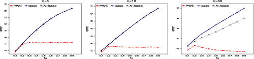
. The setup of δ0 and other parameters are presented in Setting 1 of Section 5.1. The average testing errors of the plug-in estimators and our proposed PointWise Estimator (PWE) are shown in . We can see that the errors of the plug-in estimators deteriorate quickly as r0 increases. In contrast, our proposed estimator is much less sensitive to the change of the degree of non-sparsity.
Fig. 1 The effect of nonsparsity of on plug-in estimators in terms of prediction error, where p = 1000. “A-lasso” and “lasso” denote the results of plug-in estimators with
being adaptive LASSO and LASSO, respectively, and PWE denotes the proposed method.
In typical prediction problems, a number of papers studied the convergence of prediction for various estimators, including LASSO, ridge, partial least squares, overparameterized estimators, and many others under different settings (Dalalyan, Hebiri, and Lederer Citation2017; Zhang, Wainwright, and Jordan Citation2017; Dobriban and Wager Citation2018; Bartlett et al. Citation2020, etc.). It has been observed that LASSO and related methods are less affected by the correlation strength among predictors in prediction than in estimation problems (Hebiri and Lederer Citation2013; Dalalyan, Hebiri, and Lederer Citation2017). However, for some sparse vectors for x such as , the estimation of
becomes that of the first coefficient and these methods are more affected by the correlation strength than prediction (Zou and Hastie Citation2005). All the above mentioned methods consider the plug-in estimator and the average prediction error.
Different from these existing methods, we focus on for a specific fixed x (
) rather than on estimating
and the average prediction error, where x is not required to have the same distribution as the training data. The line of works that are closely related to ours are those on the hypothesis testing and confidence intervals of
in high-dimensional linear models (van de Geer et al. Citation2014; Zhang and Zhang Citation2014; Javanmard and Montanari Citation2014; Lu et al. Citation2017; Cai and Guo Citation2017; Zhu and Bradic Citation2018, etc.). Most of these papers considered the case of
being ultra-sparse with
. Cai and Guo (Citation2017) considered the broader range where
has an order no more than
. Zhu and Bradic (Citation2018) considered the hypothesis testing and confidence intervals of
where
is allowed to be non-sparse by introducing a sparse auxiliary model, which can be restrictive. For example, if the predictor vector follows the normal distribution
and the sparse auxiliary model holds for any
simultaneously, then Σ must be equal to Ip. Moreover, the estimator of
obtained from the confidence interval of Zhu and Bradic (Citation2018), despite allowing
to be dense, works only when
in prediction problems. Although these results have optimality in the minimax sense (Cai and Guo Citation2017; Zhu and Bradic Citation2018), they can be conservative and are actually determined by the most difficult case. In this article, we introduce the sparsity of eigenvalues (or approximately low rank) of some matrices, which is shown to be complementary to the sparsity of
. The most difficult case is actually the situation where both types of sparsity fail.
Our key observation is that we can directly target at , treating it as an unknown parameter for estimation. We refer to the resulting estimate as the pointwise estimator. To this end, we propose a unified framework to leverage multiple sources of information. In many cases, the eigenvalues of the covariance matrix decrease dramatically, due to correlations among the predictors, which will be referred as sparsity of eigenvalues in the following descriptions. This type of sparsity is generally viewed as an adverse factor, making the estimation of
more difficult. Contrary to this popular view, we show that the sparsity of eigenvalues is beneficial in our framework and serves as a good complement to the sparsity of
. In practice, two different kinds of test points x are of particular interest: (a) x is a given sparse vector, and (b) x is a random vector having the same distribution as the training data (i.e., the prediction problem). We give detailed results on these two special cases and compare our estimator with several other methods. The main contribution of this article is that we propose a transformed model under a new basis, which provides a unified way to use different sources of information.
First, to use the sparsity of eigenvalues, we propose an estimator based on a basis consisting of eigenvectors of a specific matrix constructed from the training data. When the eigenvalues decrease at a certain rate, our estimator performs well for both kinds of test points x regardless of the sparsity of . On the other hand, if eigenvalues decrease slowly (or covariance matrix close to Ip), this estimator is less efficient; and consequently is inferior to LASSO when
is indeed sparse. In fact, the pointwise estimator using the sparsity of eigenvalues is complementary to LASSO.
Second, to leverage the information of , such as
being sparse, and the sparsity of eigenvalues jointly, we construct another basis based on an initial estimator
. It is shown that two types of information help each other: a faster decreasing rate of eigenvalues allows
converging in a slower rate, and vice versa. When the test point x is a sparse vector, we show that the pointwise estimator performs well. The case of x being random as in prediction problems is more complicated in the sense that the sparsity degree of
should be taken into account. Hence, we consider a subset S1 of
satisfying
, where S1 can be estimated from data. Specifically, we consider two cases: (a) Let
, which allows
to be sparse or dense. When sparsity of eigenvalues holds, our pointwise estimator performs well. When the eigenvalues are less sparse (or covariance matrix is close to Ip), our pointwise estimator performs similarly to the existing results on dense
in the literature. (b) When
is sparse, a smaller
leads to a better estimator. If a good initial estimator
and a good S1 are available, our estimator’s performance is similar to that of LASSO.
The rest of this article is organized as follows. In Section 2, we propose our pointwise estimator for the linear transformation in high-dimensional linear models. Theoretical properties are established in Sections 3 and 4. Some simulated examples and real data analysis are presented in Section 5, followed by some discussions in Section 6. Proofs of the theoretical results are provided in the Supplementary Materials.
Notation. We first introduce some notations to be used for the article. For any symmetric positive semidefinite matrix , denote the eigenvalues of A in a decreasing order as
, and the smallest nonzero eigenvalues as
. For any matrix
are the maximum and minimum singular values of A, respectively. For any vector
and
denote the
and
norms of v, respectively, and
; the support set of v is denoted as supp
. In addition, define
for any positive semidefinite matrix
. For two sequences
and
, both
and
imply
for some constant
; both
and
indicate that
;
means that an has exactly the same order as bn. For any integer i, let ei denote the vector of zeros except the ith element being 1.
2 A Unified Framework for Pointwise Estimation
Suppose , are iid from the following linear regression model
(2.1)
(2.1) where
satisfies
and
is independent of ϵi satisfying
, and
. Without loss of generality, we assume that
, and that
. Denote
, and
. Then the model can be written as
. Here the dimension p can be much larger than the sample size n. Let
be a given point at which we intend to estimate
. We assume that
for some
, which can be checked numerically. Let
of cardinality
. Since a nonsparse
and the case where Σ might not be of full rank will be considered, we make the following identifiability condition and discuss some useful facts.
When Σ is not of full rank, we assume that
falls into the column space of Σ for identifiability, due to the following reasons. Denote
The magnitude of βj;
Next we first introduce the transformed model based on a set of basis to leverage multiple sources of information in Section 2.1. The construction of basis is discussed in Section 2.2. A penalized estimator and a pointwise estimator are proposed in Section 2.3.
2.1 The Transformed Model
For any fixed , let
be the projection matrix on the space spanned by x and
be the projection matrix on the complementary space. Recall that
and denote
. Then one can write
(2.2)
(2.2) where
and
. Here αx is a scaled version of γx such that the
norm of the predictor
equals
. Estimating γx is equivalent to that of αx, since given αx, one can compute γx directly from data
. Then we get
where
is a nuisance parameter vector. Note that
is a nonsparse vector in general, particularly when Xi’s are iid variables; thus, we have n + 1 nonsparse parameters with the sample size n. To handle the difficulty, we introduce a set of basis
using different sources of information such that
can be expressed sparsely under the set of basis.
The construction of Γ depends on the information at hand and will be elaborated in Section 2.2. For an invertible matrix , of which the columns are of unit length (i.e.,
), we denote
where
. Although Γ here can be any invertible matrix, as shown later, the case we are interested in is Γ being (approximately) orthogonal. We hope that
is (approximately) sparse when Γ is chosen properly. Combining these together, we have the transformed linear model
(2.3)
(2.3) where
. The parameter
is treated as a n-dimensional nuisance parameter vector. As shown later in Section 2.2, Γ plays a critical role in this model, providing a flexible way to leverage different sources of information. A naive choice is
without using additional information, which will be discussed further in Section F of supplementary materials. In contrast to p parameters of the original linear model, the transformed model (2.3) has only n + 1 unknown parameters that are (approximately) sparse. Without loss of generality, we assume that both
and consequently
are bounded, given x and X. This assumption is mild and holds in probability when x and Xi’s are iid from
. Detailed discussions are presented in Section A of the supplementary materials.
Denote by a generic estimator of αx. Then γx can be estimated by
. Given x, noting that
, where
, we see that the quantity
affects the convergence rate of the estimator
. We investigate the magnitude of
, and consider two typical settings for clarity. Recall that x is a given vector, which may or may not have the same distribution as Xi.
Example 1.
Let x be a sparse vector with the support set and the cardinality
. Examples of such x include x = ei or
. Denote
. If the eigenvalues of
are both upper and lower bounded, and
, then it follows that
.
Example 2.
Let x be a random vector as in prediction problems. For simplicity, we assume x and Xi’s are iid variables from . As shown in Section 4.2, it follows
(2.4)
(2.4) in probability. Moreover, it holds that
and
can be viewed as the effective rank of Σ. Particularly, if some eigenvalues of Σ are much larger than the rest (e.g., the largest eigenvalue has the order p), then
; if Σ is close to Ip, then
is close to
and γx is close to
.
Clearly, the magnitude of with a sparse x in Example 1 can be smaller than that of the dense x in Example 2. If x is not sparse, the sparsity of
can help as well. This observation motivates us to consider estimators using the information of the sparsity degree of
. For any subset
such that
, we observe that
where
and
are the subvectors of x and
, respectively, and
is a p-dimensional vector obtained by setting
in x. Thus, instead of estimating γx, one can equivalently consider prediction at the point
, which is a sparse vector when
is small. Clearly, one can set
, and then
becomes γx. Estimating
provides a way to take the sparsity degree of
into account. In practice, one can choose different S1’s and select the best one by CV, as shown later in Section 2.3. In Section 4 we will compare our method with several existing methods in details for Examples 1 and 2.
Remark 1.
In Example 2 above, a smaller set S1 is preferred. However, the true support set S0 is unknown. When s0 is small, choosing a set S1 that covers S0 is feasible. For example, S1 can be taken as the support set of the LASSO estimator, or constructed by some screening methods (Fan and Lv Citation2008).
2.2 Construct Basis Utilizing Multiple Sources of Information
Next we discuss the construction of Γ. For a positive semidefinite matrix , denote
the vector of eigenvalues of A in a decreasing order. We say that
is approximately sparse when only a few eigenvalues are much larger than the average
, and the detailed requirements on the decreasing rate of eigenvalues will be elaborated later. In practice, different sources of information may be available. For clarity of the presentation, we focus on two different sources of information.
Source I. We use the information of through an initial estimator
. Note that a good estimator is available in some cases. In particular, if
is sparse, then
can be obtained from that of LASSO, or other sparse regression methods. However, an estimator
may not be good enough in many cases especially when
is less sparse and p is larger than n.
Source II. We use the dependence among predictors. Note that that equals the first n elements of
, of which the population version is
. When predictors are correlated such that
is (approximately) sparse, a key observation is that by choosing a suitable Γ, the parameter
can be (approximately) sparse regardless
being sparse or not (details are referred in Section 3.2). Thus, it is feasible to estimate the parameters well in the transformed model (2.3).
Denote , and let
. The sparsity in
is complementary to that in
. Both
and
are ideal cases with good estimators available (we will introduce estimators for Case
later), and the case
can be the least favorable case. There are intermediate cases between
and
, when the degree of sparsity of
increases gradually. A similar argument applies between
and
. To handle these complicated cases, it is natural to use these two different sources of information jointly. In fact, our approach works well under the complementary condition in Section 3.3 where stronger requirements on one type of sparsity weaken those of the other. It is possible that both
and
hold simultaneously, where our estimators leverage both sources of information.
Denote the spectral decomposition of as
where
are eigenvectors and
is the diagonal matrix of the associated eigenvalues in a deceasing order. Denote
When an initial estimator
is available,
can be estimated by
. To use two different sources of information jointly, or in other words to use both
and the columns of
, we construct Γ by replacing one of the columns (say for example the ith column) of
by
, that is,
, defined as
(2.5)
(2.5) which is the empirical version of
. More discussion on this process is provided in Proposition 1 and Remark 2.
Recall that αx, associated with predictor , is the parameter of interest in the transformed model that has predictors
. It is desirable to avoid the collinearity between zx and other predictors in the transformed model. Hence, we assume that
satisfies that
, which can be checked from data, and require the matrix
being invertible. Note that it is also required that
, that is
, is invertible.
Proposition 1.
Suppose that satisfies
and
. Then for at least one
, it holds that both matrices
and
are invertible or equivalently that
.
In principle, we can replace any by
as long as
. In our numerical studies, the strategy in Remark 2 below is used to further reduce collinearity.
Remark 2.
Reducing the collinearity between zx and other predictors in the transformed model makes the estimator of αx more stable. In our simulation studies, we replace by
with
, and the resulting
is observed nonsingular numerically.
Naturally, one can just use the information in Source II by setting . A good property for this choice is that it depends only on X without requiring an initial estimator
and is free of any assumption on the sparsity of
. However, this choice may not be ideal if a reasonably good initial estimator
can be obtained. We summarize the constructions of Γ used in this article in .
Table 1 Candidates of Γ for the pointwise estimator.
In Section 3, we show that when is sparse enough,
is approximately sparse without any sparsity assumption on
. An extreme case is Σ being a low rank matrix, where
is exactly sparse with at most
nonzero elements. It is worth pointing out that which elements of
are large are generally unknown since
is involved. When
is less sparse, as discussed below,
will provide additional information and
can still be approximately sparse.
When , the sparsity of
also depends on the accuracy of
. For the ideal case that
, it can be shown that
, and consequently
is a sparse vector. This argument still holds, if we replace
by any other vectors such that
is invertible, implying that if we know
, there is no need for additional information. Consequently, if
is good,
do not help much. When
is not good enough (e.g.,
is less sparse in particular) but
is sufficiently sparse, using
’s will compensate the low accuracy of
. Thus, both types of information can help each other in our framework and the estimator becomes more robust to the underlying assumptions. Details are provided in Section 3.
2.3 Penalized Estimator and Pointwise Estimator
As discussed in Section 2.2, the parameters in the transformed model (2.3) can be approximately sparse if Γ is constructed properly. Thus, we consider the minimization of the following objective function
(2.6)
(2.6) where
is the
penalty function used by LASSO, and λ and Γ are the tuning parameters. The parameter λ plays the same role as that for the usual regularized estimator and can be selected by cross-validation (CV). The selection of Γ will be elaborated below. Since the
penalty usually induces biases for coefficients of large absolute values, to solve this problem, other nonconvex penalty functions, such as the SCAD (Fan and Li Citation2001) or MCP (Zhang Citation2010), can be used instead. Denote the minimizer as
(2.7)
(2.7)
Then we have .
Remark 3.
Our approach involves eigenvalue decomposition of the matrix with the computational complexity of the order
, which can be a burden when n is large. To reduce the complexity, the Divide-and-Conquer (DC) approach for handling big data can be used (Zhang, Duchi, and Wainwright Citation2015). Simulation results based on DC are presented in Section G.2 of the supplementary materials.
Next we briefly discuss the estimator in (2.7). First, the predictor Z in Model (2.3) involves the transformation matrix Γ, while in the classical model (2.1), the predictor is X, of which each row represents a realization of the predictors. Second, unlike the classical methods such as the LASSO, where the parameters are unknown constants, the parameter here involves
, which makes the theoretical analysis challenging.
Remark 4.
In the above arguments, we consider a single point x that may or may not be from the same distribution as the predictor vector. However, if we are going to consider a large number of test points that are iid observations of Xi, the bias should be taken into account. Because
and
, there will be many
’s that are close to 0 and the corresponding estimators are shrunken to 0 by the penalization, resulting in large biases in terms of the average estimation error. There are many bias correction methods for LASSO and related penalized estimators in the literature (Belloni and Chernozhukov Citation2013; Zhang and Zhang Citation2014, etc.). In our simulation results for the prediction problem, the method of Belloni and Chernozhukov (Citation2013) is applied.
For clarity, we briefly summarize the estimation procedure for a given Γ as follows.
Algorithm 1
Estimator of γx (or ) with given Γ
1. (Estimate αx) Solve the optimization problem (2.6), where the optimal λ is chosen by CV; the corresponding parameter obtained is denoted as .
2. (Bias-correction) This is an optional step. Denote and
the columns of Γ with index
. Apply the OLS with responses Y and predictors
to get the updated coefficient
of
, which is a bias-corrected estimator of αx.
3. (Estimate γx) γx is estimated by
4. (Alternative Steps 1–3) Replacing x by in Steps 1–3, we get the estimator
.
Step 2 is mainly applied for the setting in Remark 4 with a large number of testing points that are iid observations as of the training data Xi’s. For clarity, the pointwise estimator obtained by Algorithm 1 is named based on the specific Γ used. There are many estimators of available for different settings in the literature, and can be used as an initial estimator. Denote by
and
the estimators of LASSO and ridge regression, respectively, and by
the overparameterized ridgeless OLS estimator using the Moore-Penrose generalized inverse (Bartlett et al. Citation2020; Azriel and Schwartzman Citation2020; Hastie et al. Citation2022). We consider the estimators
in Algorithm 1 with Γ being
and
for
, and the resulting estimators are denoted as
, respectively. Now we propose a procedure to select Γ adaptively. Denote by
a set of estimators, for example,
in Setting 1 of our numerical study. The best estimator selected from
by the following CV procedure will be denoted as PWE.
Algorithm 2
Select Γ by CV
1. Compute the CV error for estimators in . Split randomly the whole data
of size n into K parts, denoted as
. For each method
, compute the CV error,
, where
is estimated by A with data
.
2. The method A0 in with the minimum CV error is chosen to be the best one.
3. The final estimator of γx is .
For Example 1 in Section 2.1 where x is a sparse vector, we apply Algorithm 2 to get the pointwise estimator. For the prediction problems in Example 2, since the sparsity degree of is unknown, we have two choices on the subset S1: (a) simply taking
(i.e., estimate γx directly); (b) estimating S1 from data using LASSO or screening methods. Given Γ, among the candidates of S1, we can select the best one by CV, similar to Steps 1 and 2 of Algorithm 2. Note that xi should be replaced by
, which is defined in the way similar to
, when one computes the CV error in Step 1 of Algorithm 2. Moreover, one can select both Γ and S1 simultaneously by CV.
3 Properties of the Penalized Estimator
Throughout our theoretical analysis, it is assumed that ϵi’s are iid from , and
can be fixed or random and will be specified later. In this section, we present theoretical properties of the regularized estimator
in (2.7), which lays a foundation for properties of the estimator
in Section 4. To this end, we first establish results for a generic invertible matrix Γ with fixed
in Section 3.1, and then apply it to
and
in Sections 3.2 and 3.3, respectively.
3.1 A General Result on with a Generic Γ and Fixed
Recall that in Model (2.3). Let
with
It can be shown that vx is the eigenvector associated with the zero eigenvalue of
(see proof of Theorem E.1 in supplementary materials). For any
, denote
It is worth noting that
here is not the
norm of v that is defined as
; and for q = 1, they are the same. This notation
is convenient for our purpose, particularly for the discussions of the case with q = 0 or
.
For and
, denote
which measures the sparsity of the parameter
. Particularly, when q = 0, Rq is the number of nonzero elements in
. Let the tuning parameter
with
. We have the following result on a generic invertible matrix Γ.
Theorem 1.
Assume that are fixed. Let Γ be a generic invertible matrix that may depend on
. Assume the following
-sparsity condition:
for some
and some constant C > 0. Then with probability
, we have
where C1,
are positive constants. Furthermore, when Γ is a generic orthogonal matrix, the
-sparsity condition can be simplified as
for some constant
.
We make a brief discussion on the above result. First, note that , where the latter equals 1 when Γ is an orthogonal matrix. Further discussions are referred to Section A of the supplementary materials. Second, since λn has the order
, the bound of Theorem 1 does not explicitly depend on p, which is reasonable, since we have only n + 1 parameters in the transformed model (2.3). Third, the bound given above involves the sparsity of the parameter vector
in the transformed model instead of that of
, allowing
being sparse or non-sparse. As an application of Theorem 1, we present the results for Γ being
and
, respectively below.
Proposition 2.
Suppose that are fixed. Let
. Assume that the
-sparsity condition
holds for some constant C > 0. Then it holds that
with probability
, where
are positive constants.
Similar to Theorem 1, Proposition 2 allows to be sparse or non-sparse. Due to αx being bounded, we have
, which can be bounded as shown in Section 3.2. When Xi’s are random, a lower bound on
is given in Section E of the supplementary materials.
3.2 Sparsity of and Properties of when
We first show that for , if the eigenvalues of
decrease at a certain rate,
will be approximately sparse; specifically
is bounded for some
. Then we give the asymptotic results on
. Recall
are the eigenvalues of
; they are also the first n eigenvalues of
. For
and
, let
and
be the norm of the projected vector of
onto the subspace spanned by the eigenvectors of
associated with eigenvalues
,
, and
is the average magnitude of the smallest n – k eigenvalues. For any
, denote
The following Lemma 1 is a deterministic result on
.
Lemma 1.
For , it holds that
Moreover, since
in Model (2.3), it holds that
.
Generally, it is difficult to obtain the sharp upper bound in Lemma 1 without any information of eigenvalues and . Simply setting k = n, we have the trivial bound
(3.1)
(3.1) which however is unbounded and undesirable. To get better bounds on
, we take into account of the properties of eigenvalues and
, and consider the following three cases:
Case (a):
Case (b):
Case (c):
Results are presented in Corollary 1 and Proposition 3, respectively.
Corollary 1.
The following conclusions are deterministic.
1. For Case (a), it holds that for
, and
.
2. For Case (b), assume that n < p, then Thus, if
for some fixed k0, then
.
In Corollary 1, conclusion (1) holds regardless of the sparsity of , while conclusion (2) relaxes the conditions on eigenvalues by taking advantages of the sparsity of
. For Case (c), we assume that the column space of
is the same as that of Σ, accommodating the identifiability condition that
. We have the following results.
Proposition 3.
Suppose that is fixed. For Case (c) with span(
)=span(Σ), assume the following conditions: (i)
; (ii)
; (iii) n < p. Then it holds that
for all k and that
where
can be viewed as the condition number of
. For clarity, we assume that
and consider the following two specific examples of eigenvalues:
Suppose that
Denote
Condition (i) is a natural extension of the condition for fixed
in Section 2. Condition (ii) is mild, ruling out the extreme case that Σ has eigenvalues
. Details are referred to the proof in supplementary materials. The two examples in Proposition 3 imply that
can be approximately sparse, when eigenvalues decrease fast enough. Based on the results of
in Corollary 1 and Propositions 3, by applying the conclusion of Proposition 2, we are ready to give the asymptotic results of
.
Theorem 2.
Suppose that are fixed. Taking
, we have the following conclusions for Cases (a)–(c):
For Case (a),
For Case (c) of a dense
The condition above can be checked from data. Here k0 and
reflect the sparsity of the parameters in the transformed model. Faster decay rates of eigenvalues result in smaller values of k0 and
, and consequently better convergence rates of
. Moreover, a smaller value of q results in a smaller value of
, but requires a faster decreasing rate of eigenvalues. Note that the above bounds only depend on n and the degree of sparsity in eigenvalues, and do not explicitly depend on p. Moreover, for Cases (a) and (c) where
is allowed to be dense, the sparsity of eigenvalues is complementary to the sparsity of
.
3.3 Properties of the Regularized Estimator with an Initial
We study properties of our estimator with , giving the convergence rate of
, for fixed x and Xi’s being iid from
. The normality assumption of Xi’s simplifies the proofs and can be relaxed to general distributions such as sub-Gaussian distributions. We first give a result on
. Recall that
.
Proposition 4.
Assume that x is fixed, Xi’s are iid from , and
. For any estimator
in Model (2.1), it holds that
. Assuming further that
, then
.
When is the LASSO estimator, we have
with
(Bickel, Ritov, and Tsybakov Citation2009), and consequently
. Let
be the function obtained by setting q = 1 in
defined in Section 3.2.
Theorem 3.
Let . Assume that following conditions: (i) Xi’s are iid from
, x is fixed, and n < p; (ii)
satisfies
and
is obtained from additional data independent of
, satisfying
. Then it holds that
, where
. Assuming further the Complementary condition:
, it follows that
.
Based on the proof, one can see that and
in Theorem 3 can be replaced by
and
respectively. The assumption on
in (ii) is mild as
and
is bounded in probability. We give some examples on the magnitude of
.
Corollary 2.
(a) If Σ is of low rank, say , then
. (b) Suppose that
for some fixed k0 and that
. Then
. (c) Suppose that
and denote
. Assuming that
decreases exponentially in probability, that is,
for
, where
, then
.
Proof of Corollary 2
is similar to those of Corollary 1 and Proposition 3 and is omitted. We point out two basic facts: from (3.1), and
by Condition (ii) and the law of large numbers. Moreover, the error rate of an estimator is generally believed having an order no less than
; thus, without loss of generality we have
throughout this article. Hence, Theorem 3 leads to the error rate of order
in probability without any restriction on the decay rate of eigenvalues.
The complementary condition involves two terms, and
, where the former is controlled by the decay rate of the eigenvalues, and the latter depends on the accuracy of
. As argued before, as long as the eigenvalues decrease fast,
will be bounded, even if
. Therefore, if
is not accurate but eigenvalues decay fast, we can still get good results. The same argument applies when
is accurate but the eigenvalues decay slowly. Particularly, if
is good enough such that
, then the requirement on the decaying rate of eigenvalues can be removed completely. Thus, the information of
and eigenvalues are complementary to each other, requiring only the product of
and
being bounded. Theorem 3 assumes
being independent of the data
. When
depends on
, we get a similar result on
with some modifications on the Condition (i), which is presented in Section F of the supplementary materials.
4 Results of for Two Types of Test Points
In Section 3, we establish theoretical properties of . With
, it is natural to get the corresponding results on
for a generic x. As mentioned in Examples 1 and 2 in Section 2.1, we are interested in two typical settings in particular: (a) x is a sparse vector with
and
, and (b) x is a random vector as an iid copy of Xi (i.e., the prediction problem). Next we give the theoretical results on
for these two examples, based on the simple fact that
.
4.1 Properties of for a Sparse x
Proposition 5.
Assume the following conditions: (i) x is a fixed sparse vector satisfying ; (ii)
, where
is formed by the columns of X with index Sx. Then we have
. Moreover, the following results hold.
Take
Let
The condition is a type of the restricted eigenvalue condition (Bickel, Ritov, and Tsybakov Citation2009). If Xi’s are iid variables,
. Recall that
in Case (a) of Theorem 2; then the condition
implies that
there.
Remark 5.
We briefly discuss the case of or close to Ip for a sparse vector x. For
, using the trivial bound in (3.1) on Rq and taking q = 1 in Proposition 2, we can see that the error of
has the order
, and consequently
.
We briefly compare our method with the plug-in estimator using the LASSO estimator (named briefly as LASSO). For LASSO, the error varies depending on the direction of x, while results of our estimator depend only on the sparsity degree sx of x. For simplicity of comparison, we consider a bound of LASSO depending only on sx. Specifically, as
, we have
(Bickel, Ritov, and Tsybakov Citation2009); the latter will be used as the error rate of LASSO. Recall that
denote our estimator with
. For Case (a), it follows from Proposition 5 that
is better than LASSO if and only if
. Cases (b) and (c) can be analyzed similarly. Recall that
is our estimator with
.
Corollary 3.
Denote by the ratio of error rate of
over that of LASSO for a fixed sparse x. Suppose that the conditions (i) and (ii) in Proposition 5 and the conditions of Theorem 3 hold. Then
has the error rate of order
and consequently
. If
, then
, impliying
is superior to LASSO; otherwise
is inferior or similar to LASSO.
The proof of Corollary 3 is a simple combination of Proposition 4 and (2) of Proposition 5 and is omitted here. Since we always have , the requirement
is mild.
4.2 Properties of for Prediction Problems
In a prediction problem, x and Xi’s are iid variables. Recall that .
Proposition 6.
Suppose that x and Xi’s are iid from . Then
In addition, it holds that
. Particularly,
when Σ is of low rank, and
when
.
Next we first derive properties of with
. Then we consider the estimator
with
, given both an initial estimator
and a subset S1.
4.2.1 Properties of for x in Prediction with
Recall that . Combining Proposition 6 and the result on
with fixed
given in Proposition 2 for
, it can be inferred that
. Clearly, a faster decay rate of the eigenvalues
leads to a smaller value of
, and a faster decay rate of ψi’s or equivalently a smaller value of Rq, consequently a better rate. Different from the fixed
considered in Theorem 2,
are random variables in this section. Thus, Rq lacks an explicit rate, due to randomness of the empirical eigenvalues ψi’s. The magnitudes of ψi’s, though can be checked from data, are hard to extract in theory generally, according to random matrix theory. To the best of our knowledge, there is no solution for a general case. To obtain an explicit result, we consider two extreme cases: (a) Σ is (approximately) low rank; (b)
, the least favorable case.
Proposition 7.
Suppose that x and Xi’s are independent from . Assume that n < p. Taking
, we have the following conclusions:
If Σ is of low rank with
For the least favorable case of
For the case of Σ having a low rank, has the order similar to that of
. But when
, the error diverges, which is not surprising since
is nonsparse in the transformed model in this setting and the rate is determined by the most difficult case. Particularly, the rate for
is the combination of the facts that
and
. Next we briefly compare LASSO with the proposed method with
. LASSO performs well in prediction when
is (approximately) sparse, and is less sensitive to the sparsity of eigenvalues. In contrast, the proposed method with
has good performance when the eigenvalues of Σ decrease fast, and
can be sparse or less sparse. Thus, our method with
and LASSO are complementary to each other.
4.2.2 Error of in Prediction with
Recall that in Example 2 in Section 2.1, for any
with
, implying that one can make prediction at the point
. Trivially, one can take
such that
. The subset S1 takes the sparsity degree of
into account. Given an initial estimator
and a subset S1 such that
, by applying our approach with
that is constructed with x replaced by
, we obtain the estimator of
denoted as
.
Denote , which stands for the prediction error of an initial estimator
. Without loss of generality, we assume
has magnitude of order no less than
. Let
and
with
standing for the effective rank of matrix
. Let
be the quantity defined similar to
but with the eigenvalues of
, satisfying
(the detailed expression is given in the supplementary materials). We have the following conclusions from Theorem 3.
Theorem 4.
Let . Assume that (i) x and Xi’s are iid variables from
and n < p; (ii) Both S1 and
are independent of
satisfying
. Then it holds that
. If we further assume the complementary condition:
, it holds that
. These conclusions are still valid for
.
Theorem 4 shows that the rate depends on , and
. The first two depend on the decay rate of eigenvalues. Moreover, it holds that
by the assumptions that both
and
are bounded, which imposes restrictions on
. Hence, by Theorem 4, without the complementary condition, we have the error rate
.
We compare with the plug-in method using LASSO estimator
(briefly named LASSO). By the typical rate of LASSO, we have
. To simplify the comparison, we assume that the LASSO estimator is consistent, that is,
. Then one can see that the condition
becomes
, which is mild, since it always holds that
.
Denote by the ratio of the error rate of
over
for random test points. Then
would imply that our method is better than LASSO. By Theorem 4, we see that
in probably. To investigate the magnitude of the latter, we consider the following two cases:
Suppose that
If we simply set
5 Numerical Studies
We use simulation studies in Section 5.1 and real data analysis in Section 5.2 to further illustrate the numerical performance of our method.
5.1 Simulations
We consider the simulation studies with samples generated iid from the linear model (2.1) with p = 1000 dimensional vector and
. Set
with
, where η controls the level of dependence strength among the predictors, with larger values of η implying stronger correlations among predictors. For the convenience of discussion, the plug-in estimator is named by the method used in estimating
. For example, “LASSO,” “ridge,” and “ridgeless” denote the plug-in estimators
with
being LASSO, ridge and ridgeless estimators, respectively.
Setting 1 (Prediction). We set , where
is the p0-dimensional vector of 1, and
such that
. Clearly,
is denser for larger values of r0, and we set
. For prediction, we set
for Algorithm 2 in Section 2.3.
We compare the prediction performance of different methods. Split the data into two parts with the training sample of size ntr = 200 and the testing sample of size nte = 500 to compute the test error. PWE estimators are obtained by Algorithm 2 with the given above and
. For the implementation of Algorithm 1, the bias correction step is adopted. We repeat the procedure 100 times and calculate the average test error for each method. We compare LASSO, ridge, ridgeless,
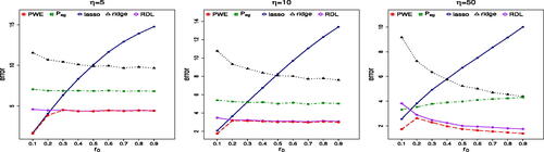
and the PWE estimators. For clarity, simulation results for Setting 1 are summarized as follows:
Comparison of LASSO, ridge, ridgeless with PWE and
Comparison of plug-in estimators with our proposed pointwise counterparts. Due to the limited space, the results are presented in in Section G.1 of the supplementary material. It is seen that the performance of
Fig. 2 Simulation prediction results of PWE, LASSO, ridge, , and ridgeless (RDL).
Setting 2 (Sparse linear transformation). We consider x being sparse vectors in . Set
, where
. Consider γx being one of the four quantities β1,
, βp and
, corresponding to taking x being
and
, respectively in γx. Note that
, indicating that there is no difference between effects of the first and third predictors;
and
stand for strong and weak signals, respectively. Moreover,
indicates that the pth predictor is insignificant. Let
and
with
, so that the predictors are highly correlated. We set the training data size ntr = 150, and compute the average errors of
over 100 replications. We compare the regularized estimators,
, and
, with the plug-in ones. Estimation comparison results are presented in .
Table 2 The average values of .
For a strong signal β1, it can be inferred from that the regularized pointwise estimators and
are better than LASSO, adaptive LASSO and ridge regression. For weak signal
, ridge estimator is better than others. The main reason is that other methods sometimes shrink the estimators to zero, resulting in large biases. For
, except ridge regression, other methods give zero estimates. Finally, for
, all the regularized pointwise estimators result in exactly zero estimates, while the plug-in estimators LASSO and adaptive LASSO lead to large biases.
Setting 3 (Comparison on different subset S1). As pointed out in Sections 2.1 and 2.3, one can consider prediction at the point instead of x in prediction problems. Under the setup of Setting 1, we take
and compare the following four candidates of S1: (1) S1 being
, which is the ideal case; (2) S1 being
, that is,
; (3) S1 is obtained by SIS of Fan and Lv (Citation2008), denoted as
; (4) S1 being the
. For each candidate of S1, we repeat 100 times and report the average values of the prediction error, true positive rate (TP) and the average length (LEN) that are defined as TP=
and LEN=
, respectively.
Due to the limited space, we present the simulation results in Section G.2 in supplementary materials. It is seen that S0 always leads to the best prediction errors in all cases. When where
is very sparse, both
and
have higher values of TP and smaller values of LEN, leading to smaller prediction errors than those of
. As r0 increases, the signal of βj’s becomes weak due to the constraint
, and the values of TP for
are very small and are the smallest ones among all subsets, which lead to the worst prediction errors. On the other hand, TP and consequently errors of
are much better than those of
, because LASSO takes into account correlations among the predictors when selecting the significant variables, while SIS uses only the marginal correlations. In addition, it is observed that
performs similar to that of
, which is partially due to the following reason. During the construction of
with a given S1, we need to compute
, which equals
for S1 being both
and
.
Setting 4 (Further comparison for heterogeneous test points). In Setting 1 where test points are iid copies from the training distribution, is nearly the same as LASSO when η is small such as η = 5 (results shown in in supplementary material). We compare them further for the case of xi’s following a distribution different from Xi’s, which is known as covariate shift in the literature of transfer learning (Weiss, Khoshgoftaar, and Wang Citation2016). We generate training data of size 100 as in Setting 1 with η = 5 and
with
. The test points xi’s are iid from
. The eigenvectors matrix
of
is uniformly distributed on the set of all orthogonal matrices in
. The eigenvalues of
, denoted as
, satisfy that
such that
. We first generate a
and then 200 test points with given
, and repeat this procedure 100 times to compute average prediction errors. Results in show that
is much better than LASSO for the case of covariate shift even for small η, possibly due to the flexible pointwise prediction of our proposed method. Besides these examples, additional results demonstrate that
can also substantially improve the ridgeless estimator when covariate shift exists for testing data (Section G.1 of supplementary materials).
Table 3 Test errors of LASSO and with η = 5 for testing points from
.
5.2 Real Data Analysis
We apply our method to a dataset from the Alzheimer’s Disease Neuroimaging Initiative (ADNI) (https://adni.loni.usc.edu/). Alzheimer’s Disease (AD) is a form of dementia characterized by progressive cognitive and memory deficits. The Mini Mental State Examination (MMSE) is a very useful score in practice for the diagnosis of AD. Generally, any score greater than or equal to 27 points (out of 30) indicates a normal cognition. Below this, MMSE score can indicate severe ( points), moderate (10–18 points) or mild (19–24 points) cognitive impairment (Mungas Citation1991). Currently, structural magnetic resonance imaging (MRI) is one of the most popular and powerful techniques for the diagnosis of AD. One can use MRI data to predict the MMSE score and identify the important diagnostic and prognostic biomarkers. The dataset we used contains the MRI data and MMSE scores of 51 AD patients and 52 normal controls. After the image preprocessing steps for the MRI data, we obtain the subject-labeled image based on a template with 93 manually labeled regions of interest (ROI) (Zhang and Shen Citation2012). For each of the 93 ROI in the labeled MRI, the volume of gray matter tissue is used as a feature. Therefore, the final dataset has 103 subjects. For each subject, there are one MMSE score and 93 MRI features. We treat the MMSE score as the response variable and MRI features as predictors.
We split the data at random with 80% as the training set, denoted as , and 20% as the testing set, denoted as
, then compute the average test error
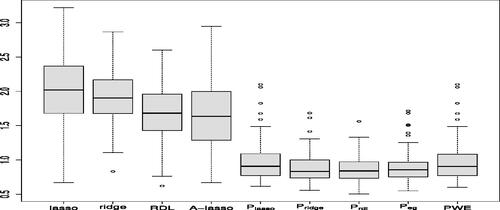
. We repeat the procedure for 100 times and report the average test errors. The boxplots of different methods are presented in . It shows that pointwise estimators are much better than plug-in estimators of LASSO, adaptive LASSO and ridge, respectively.
Fig. 3 Comparison of the test errors of different methods for the AD data analysis. Here , and
represent our regularized estimators without bias-correction in Algorithm 1. The PWE is automatically selected from
, and
.
6 Discussion
In this article, we estimate the linear transformation of parameters
in high-dimensional linear models. We propose a pointwise estimator, which works well when
is sparse or non-sparse, and predictors are highly or weakly correlated. The theoretical analysis reveals the significant difference between estimating a linear transformation of
and that of
. When
is non-sparse or predictors are highly correlated, estimating
is difficult, but we can still get good estimate of
using our proposed pointwise estimators.
Supplementary Materials
The supplementary materials contain two parts. The first part provides the proofs of the theoretical results in the main paper. The second part includes some simulation results for the settings 2 and 3 of the main paper, together with additional simulation results.
Supplemental Material
Download Zip (768.7 KB)Acknowledgments
The authors would like to thank the Editor, the Associate Editor, and reviewers, whose helpful comments and suggestions led to a much improved presentation.
Additional information
Funding
Related Research Data
References
- Azriel, D., and Schwartzman, A. (2020), “Estimation of Linear Projections of Non-Sparse coefficients in High-Dimensional Regression,” Electronic Journal of Statistics, 14, 174–206. DOI: 10.1214/19-EJS1656.
- Bartlett, P. L., Long, P. M., Lugosi, G., and Tsigler, A. (2020), “Benign Overfitting in Linear Regression,” Proceedings of the National Academy of Sciences, 117, 30063–30070. DOI: 10.1073/pnas.1907378117.
- Belloni, A., and Chernozhukov, V. (2013), “Least Squares after Model Selection in High-Dimensional Sparse Models,” Bernoulli, 19, 521–547. DOI: 10.3150/11-BEJ410.
- Bickel, P. J., Ritov, Y., and Tsybakov, A. B. (2009), “Simultaneous Analysis of Lasso and Dantzig Selector,” The Annals of Statistics, 37, 1705–1732. DOI: 10.1214/08-AOS620.
- Bühlmann, P., and Van De Geer, S. (2011), Statistics for High-Dimensional Data: Methods, Theory and Applications, Berlin: Springer.
- Cai, T. T., and Guo, Z. (2017), “Confidence Intervals for High-Dimensional Linear Regression: Minimax Rates and Adaptivity,” The Annals of Statistics, 45, 615–646.
- Dalalyan, A. S., Hebiri, M., and Lederer, J. (2017), “On the Prediction Performance of the Lasso,” Bernoulli, 23, 552–581. DOI: 10.3150/15-BEJ756.
- Dobriban, E., and Wager, S. (2018), “High-Dimensional Asymptotics of Prediction: Ridge Regression and Classification,” The Annals of Statistics, 46, 247–279. DOI: 10.1214/17-AOS1549.
- Fan, J., and Li, R. (2001), “Variable Selection via Nonconcave Penalized Likelihood and its Oracle Properties,” Journal of the American Statistical Association, 96, 1348–1360. DOI: 10.1198/016214501753382273.
- Fan, J., and Lv, J. (2008), “Sure Independence Screening for Ultrahigh Dimensional Feature Space,” Journal of the Royal Statistical Society, Series B, 70, 849–911. DOI: 10.1111/j.1467-9868.2008.00674.x.
- Hastie, T., Montanari, A., Rosset, S., and Tibshirani, R. J. (2022), “Surprises in High-Dimensional Ridgeless Least Squares Interpolation,” The Annals of Statistics, 50, 949–986. DOI: 10.1214/21-aos2133.
- Hebiri, M., and Lederer, J. (2013), “How Correlations Influence Lasso Prediction,” IEEE Transactions on Information Theory, 59, 1846–1854. DOI: 10.1109/TIT.2012.2227680.
- Javanmard, A., and Montanari, A. (2014), “Confidence Intervals and Hypothesis Testing for High-Dimensional Regression,” The Journal of Machine Learning Research, 15, 2869–2909.
- Lu, S., Liu, Y., Yin, L., and Zhang, K. (2017), “Confidence Intervals and Regions for the Lasso by Using Stochastic Variational Inequality Techniques in Optimization,” Journal of the Royal Statistical Society, Series B, 79, 589–611. DOI: 10.1111/rssb.12184.
- Mungas, D. (1991), “In-Office Mental Status Testing: A Practical Guide,” Geriatrics, 46, 54–67.
- Negahban, S. N., Ravikumar, P., Wainwright, M. J., and Yu, B. (2012), “A Unified Framework for High-Dimensional Analysis of m-estimators with Decomposable Regularizers,” Statistical Science, 27, 538–557. DOI: 10.1214/12-STS400.
- Raskutti, G., Wainwright, M. J., and Yu, B. (2011), “Minimax Rates of Estimation for High-Dimensional Linear Regression over lq -balls,” IEEE Transactions on Information Theory, 57, 6976–6994.
- Tibshirani, R. (1996), “Regression Shrinkage and Selection via the Lasso,” Journal of the Royal Statistical Society, Series B, 58, 267–288. DOI: 10.1111/j.2517-6161.1996.tb02080.x.
- van de Geer, S., Bühlmann, P., Ritov, Y., and Dezeure, R. (2014), “On Asymptotically Optimal Confidence Regions and Tests for High-Dimensional Models,” Annals of Statistics, 42, 1166–1202.
- Weiss, K., Khoshgoftaar, T. M., and Wang, D. (2016), “A Survey of Transfer Learning,” Journal of Big Data, 3, 1–40. DOI: 10.1186/s40537-016-0043-6.
- Zhang, C. H. (2010), “Nearly Unbiased Variable Selection Under Minimax Concave Penalty,” Annals of Statistics, 38, 894–942.
- Zhang, C. H., and Zhang, S. S. (2014), “Confidence Intervals for Low Dimensional Parameters in High Dimensional Linear Models,” Journal of the Royal Statistical Society, Series B, 76, 217–242. DOI: 10.1111/rssb.12026.
- Zhang, D., and Shen, D. (2012), “Multi-Modal Multi-Task Learning for Joint Prediction of Multiple Regression and Classification Variables in Alzheimer’s Disease,” Neuroimage, 59, 895–907. DOI: 10.1016/j.neuroimage.2011.09.069.
- Zhang, Y., Duchi, J., and Wainwright, M. (2015), “Divide and Conquer Kernel Ridge Regression: A Distributed Algorithm with Minimax Optimal Rates,” The Journal of Machine Learning Research, 16, 3299–3340.
- Zhang, Y., Wainwright, M. J., and Jordan, M. I. (2017), “Optimal Prediction for Sparse Linear Models? Lower Bounds for Coordinate-Separable m-estimators,” Electronic Journal of Statistics, 11, 752–799. DOI: 10.1214/17-EJS1233.
- Zhu, Y., and Bradic, J. (2018), “Linear Hypothesis Testing in Dense High-Dimensional Linear Models,” Journal of the American Statistical Association, 113, 1583–1600. DOI: 10.1080/01621459.2017.1356319.
- Zou, H., and Hastie, T. (2005), “Regularization and Variable Selection via the Elastic Net,” Journal of the Royal Statistical Society, Series B, 67, 301–320. DOI: 10.1111/j.1467-9868.2005.00503.x.