Survival Mixed Membership Blockmodel

Abstract

Whenever we send a message via a channel such as E-mail, Facebook, WhatsApp, WeChat, or LinkedIn, we care about the response rate—the probability that our message will receive a response—and the response time—how long it will take to receive a reply. Recent studies have made considerable efforts to model the sending behaviors of messages in social networks with point processes. However, statistical research on modeling response rates and response times on social networks is still lacking. Compared with sending behaviors, which are often determined by the sender’s characteristics, response rates and response times further depend on the relationship between the sender and the receiver. Here, we develop a survival mixed membership blockmodel (SMMB) that integrates semiparametric cure rate models with a mixed membership stochastic blockmodel to analyze time-to-event data observed for node pairs in a social network, and we are able to prove its model identifiability without the pure node assumption. We develop a Markov chain Monte Carlo algorithm to conduct posterior inference and select the number of social clusters in the network according to the conditional deviance information criterion. The application of the SMMB to the Enron E-mail corpus offers novel insights into the company’s organization and power relations. Supplementary materials for this article are available online.

KEYWORDS:

• Model identifiability
• Semiparametric cure rate model
• Social networks
• Time-to-event data

1 Introduction

With the rapid development of social media and electronic commerce, many social networks now encompass a sequence of time-to-event data for a pair of social actors. In an E-mail network, how long it takes for the receiver of an E-mail to reply to the sender is available; on Twitter and Sina Weibo, the time for a user to repost a message from another user can be recorded; in a company that uses web-based electronic document management systems such as those provided by Dropbox and ParaDM, the time an employee processes a file shared by another employee can be tracked. Compared to the number of events between a pair of actors, time-to-event data can provide alternative perspectives into interpersonal relationships. For instance, an employee may have many more E-mails with a secretary than with the CEO but replies to E-mails from the CEO much faster than to those from the secretary. However, despite the active research on time-to-event data on social networks, statistical research on response times and response rates on a social network is still lacking.

Many previous studies on time-to-event data from a social network focus on the behavior undertaken by a social actor to initiate events, either by sending E-mails or by posting tweets. Such behavior has often been modeled by point processes. Perry and Wolfe (2013) treat the time of sending E-mails between pairs of actors in a network as a multivariate point process. Fox et al. (2016) adopt self-exciting point processes to model the rate of sending E-mails, in which the intensity function comprises a baseline sending rate and triggering functions that characterize the impact of receiving E-mails on sending rates. Matias, Rebafka, and Villers (2018) assume that each actor belongs to one and only one social group, in line with the classical stochastic blockmodel (Wang and Wong 1987), and assume a separate conditional inhomogeneous Poisson process for each social group pair. They use the proposed model to analyze the times at which actor A sends E-mails to actor B. Sit, Ying, and Yu (2021) model the times that an actor A sends an E-mail to actor B as recurrent events and develop a pseudo-partial likelihood approach to capture the flexible dependence structures among pairs of actors in the network. Zhang et al. (2022) jointly model the times at which actors initiate two events: posting their own tweets and reposting tweets from others. All of these studies focus on how frequently actor A initiates events (such as by posting tweets) or how frequently actor A interacts with actor B (such as by sending an E-mail to actor B).

Nevertheless, we not only care how frequently friends or colleagues contact us, but we are also always eager to know (a) whether the recipient will reply to our message (response rate) and (b) how long it will take us to receive a reply (response time). Both the response rate and the response time encode important information. For example, even if two actors send E-mails with a similar frequency, the one with a higher response rate will be more influential in their social network. Therefore, instead of studying the sending behaviors, in this article, we will model response rates and response times on a social network.

Noteworthy, the response behavior of actors in a social network can be highly heterogeneous. Recently, Rastelli and Fop (2020) propose the exponential stochastic blockmodel (expSBM) to examine the duration of the interaction between actors. expSBM assumes that the network structure follows the stochastic blockmodel (Wang and Wong 1987) and that the interaction lengths follow exponential distributions. To fit into their framework, we may view actors’ E-mail response behaviors as interactions and the time period with no E-mail and with no E-mail reply as a noninteraction period. Because the stochastic blockmodel partitions the network into several communities and lets each actor belong to one and only one community, although expSBM allows individuals’ response speed to vary, it assumes the response speed of a given social actor to be the same no matter whom he or she interacts with. However, even for the same person, his or her response speed can be very different when communicating with different people. For example, the speed of an employee’s responses to the CEO, a secretary, and his or her peers can vary considerably. Moreover, expSBM cannot deal with censoring time and hence E-mails that are never replied to.

To deal with the challenges of nonresponse events, severe heterogeneity, and sparse observations, we integrate the mixed membership stochastic blockmodel (MMSB) (Airoldi et al. 2008) with the semiparametric cure rate model (SCRM) (Chen, Ibrahim, and Sinha 1999; Ibrahim, Chen, and Sinha 2001a, chap. 5) to build a survival mixed membership blockmodel (SMMB). The SMMB allows an actor to play different roles when interacting with different actors, accounts for the impact of covariates, and models nonresponse events. Globally, the SMMB can detect social clusters in a network and characterize between- and within-cluster interaction patterns. Locally, the SMMB is capable of identifying the specific role an actor plays when he or she interacts with another actor. The SMMB simultaneously learns the network structure from the data and uses the learned structure to improve actor pair-specific inference. Consequently, the SMMB pools information across the whole network.

The network structure inferred from time-to-event data can be very different from the structure learned from a binary network W that records the connectivity between actors. In this article, we use “communities” to refer to the grouping of actors according to their connectivity encoded by W and “roles” to refer to the grouping of actors according to their response times and response rates. If W follows an MMSB, then actors belonging to the same community have a high probability of communicating with each other—sending E-mails in the case of the Enron E-mail corpus. In comparison, actors sharing the same role have similar distributions of response times and response rates in the SMMB. Therefore, communities and roles reveal different aspects of a social network with time-to-event data. For example, different communities can correspond to the various departments of a company, whereas roles reflect employees’ levels of seniority. Employees in the same department tend to have more E-mail contacts, and thus are grouped together by W, but have very different E-mail response speeds and rates because of their different levels of seniority.

As pointed out by Zhang, Levina, and Zhu (2020), it is nontrivial to establish identifiability for social network models that allow actors to belong to multiple social clusters such as the MMSB (Airoldi et al. 2008). Recently, Mao, Sarkar, and Chakrabarti (2021) prove that the requirement of the existence of at least one pure node, defined as a social actor who acts as a member of only one social cluster irrespective of whom he or she communicates with, for each social cluster is not only sufficient (Kaufmanna, Bonaldb, and Lelargec 2018; Zhang, Levina, and Zhu 2020) but also necessary for the MMSB for binary networks to be identifiable. Fortunately, compared with binary data, time-to-event data encode more information, and hence we are able to prove that the SMMB is identifiable up to label switching without the pure node assumption.

We conduct statistical inference under the Bayesian framework and develop a Markov chain Monte Carlo (MCMC) algorithm. The application of the SMMB to the Enron E-mail corpus reveals network structure that better represent leadership patterns than those obtained from the state-of-the-art methods.

2 Model Formulation

Suppose that a social network consists of N actors and has sequences of time-to-event data, instead of binary outcomes W_ijs, recorded for actor pairs. For a pair of actors (i, j), when actor i sends a sequence of E-mails to actor j, the response (failure) time and the censoring time for the gth E-mail by actor j are denoted as T_ijg and C_ijg, respectively. The associated p-dimensional covariates are denoted as ${\mathit{X}}_{\mathit{ijg}}={(X_{\mathit{ijg}1},X_{\mathit{ijg}2},\dots ,X_{\mathit{ijgp}})}^T$, where $X_{\mathit{ijg}1}=1$ corresponds to the intercept term. If actor i sends n_ij E-mails to actor j, then we observe a sequence of survival times ${\mathit{y}}_{ij}={(y_{ij1},\dots ,y_{ij{n}_{ij}})}^T$ and censoring indicators ${\mathit{\nu }}_{ij}={({\nu }_{ij1},\dots ,{\nu }_{ij{n}_{ij}})}^T$ satisfying $y_{\mathit{ijg}}=\min (t_{\mathit{ijg}},c_{\mathit{ijg}})$ and ${\nu }_{\mathit{ijg}}=\mathbf{1}(t_{\mathit{ijg}}<c_{\mathit{ijg}})$, and the corresponding covariates ${\mathit{x}}_{ij}={({\mathit{x}}_{ij1},\dots ,{\mathit{x}}_{ij{n}_{ij}})}^T$. Here, $\mathcal{N}=\{1,\dots ,N\}$ denotes the set of actors and $\mathcal{E}=\{(i,j)|n_{ij}>0,i,j\in \mathcal{N}\}$ represents the set of actor pairs with at least one failure or censoring observation.

Following the MMSB, assume that there exist K roles with Dirichlet parameters $\mathit{\xi }={({\xi }_1,\dots ,{\xi }_K)}^T\in {(0,+\infty )}^K$. Here, $\frac{{\xi }_k}{{\sum }_{l=1}^K{\xi }_l}$ represents the abundance of the kth role in the network. Each pair of roles has a unique SCRM.

For the SCRM, we adopt the formulation $S(t) =\hspace{0.17em}\exp \hspace{0.17em}(-\theta +\theta S_0(t))={\tau }^{1-S_0(t)}$ (Chen, Ibrahim, and Sinha 1999; Ibrahim, Chen, and Sinha 2001a, chap. 5), which enjoys a population level proportional hazards structure. Here, $S_0(t)$ is a proper survival function for the baseline, and its hazard function $h_0(t)$ is piecewise constant: $h_0(t)={\lambda }_m$ if $t\in (s_{m-1},s_m]$, with $0<s_1<s_2<\cdots <s_M<\infty$ being a partition of the time axis and $h_0(t)=0$ for $t>s_M$. Meanwhile, $\tau =\hspace{0.17em}\exp \hspace{0.17em}(-\theta )$ is the cure proportion. The survival time of this model can be viewed as the earliest event time of $\tilde{N}$ iid competing risks with survival probability $S_0(t)$ and $\tilde{N}$ following a Poisson distribution $\text{Pois}(\theta )$, so θ can be interpreted as the average number of competing risks (Chen, Ibrahim, and Sinha 1999). Similarly, we may suppose that there exist $\tilde{N}$ latent intentions to reply to an E-mail and view θ as the average number of latent response intentions. Furthermore, we can model covariate effects $\mathit{\beta }={({\beta }_1,\dots ,{\beta }_p)}^T$ via $\theta =\hspace{0.17em}\exp \hspace{0.17em}({\mathit{x}}^T\mathit{\beta })$, which corresponds to a log-log link for τ: $\hspace{0.17em}\log \hspace{0.17em}(-\hspace{0.17em}\log \hspace{0.17em}(\tau ))={\mathit{x}}^T\mathit{\beta }$. Consequently, the hazard function of the SCRM is $h(t|\mathit{x})=\hspace{0.17em}\exp \hspace{0.17em}({\mathit{x}}^T\mathit{\beta })f_0(t)$, where $f_0(t)$ denotes the probability density function for $S_0(t)$. In the SMMB, we let both the baseline hazards and covariate effects to be role-pair-specific.

When role k replies to the E-mails sent by role l, the piecewise constant baseline hazard function in interval $t\in (s_{m-1},s_m]$ is $h_0^{lk}(t)={\lambda }_m^{lk}$. We collect ${\mathit{\lambda }}^{lk}=({\lambda }_1^{lk},\dots ,{\lambda }_M^{lk})$ and denote the role-pair-specific covariate effects as ${\mathit{\beta }}^{lk}={({\beta }_1^{lk},\dots ,{\beta }_p^{lk})}^T$. Notably, the time-to-event data from role l to role $k\ne l$ do not necessarily have the same distribution as those from role k to role l. In other words, $f^{lk}(y,\nu |\mathit{x},{\mathit{\beta }}^{lk},{\mathit{\lambda }}^{lk})=f^{kl}(y,\nu |\mathit{x},{\mathit{\beta }}^{kl},{\mathit{\lambda }}^{kl})$ is not required. Instead, the interactions are allowed to be asymmetric.

When actor j replies to an E-mail sent by actor i, actor i and actor j pick up their latent social role Q_ij and R_ij according to their latent role proportions ${\mathit{\pi }}_i={({\pi }_{i1},\dots ,{\pi }_{iK})}^T$ and ${\mathit{\pi }}_j$, respectively. Given the latent roles $Q_{ij}=l$ and $R_{ij}=k$, a sequence of failure times $T_{\mathit{ijg}},g=1,\dots ,n_{ij}$ are iid generated according to a SCRM with the piecewise constant baseline hazards ${\mathit{\lambda }}^{lk}$ and the coefficients ${\mathit{\beta }}^{lk}$.

We denote $\mathit{\xi }={({\xi }_1,\dots ,{\xi }_K)}^T,\mathit{\beta }={\left\{{\mathit{\beta }}^{lk}\right\}}_{k=1,\dots ,K}^{l=1,\dots ,K}$ and $\mathbf{\Lambda }={\left\{{\mathit{\lambda }}^{lk}\right\}}_{k=1,\dots ,K}^{l=1,\dots ,K}$. The proposed SMMB can then be described by the following data generation mechanism: (1) $$\begin{array}{c}{\mathit{\pi }}_i\sim \text{Dirichlet}(\mathit{\xi })i=1,\dots ,N;\\ Q_{ij}|{\mathit{\pi }}_i\sim \text{Categorical}({\mathit{\pi }}_i)(i,j)\in \mathcal{E};\\ R_{ij}|{\mathit{\pi }}_j\sim \text{Categorical}({\mathit{\pi }}_j)(i,j)\in \mathcal{E};\\ Y_{\mathit{ijg}},{\nu }_{\mathit{ijg}}|Q_{ij}=l,R_{ij}=k\sim f(y_{\mathit{ijg}},{\nu }_{\mathit{ijg}}|Q_{ij}=l,R_{ij}=k,{\mathit{x}}_{\mathit{ijg}},\mathit{\beta },\mathbf{\Lambda })\\ =f(y_{\mathit{ijg}},{\nu }_{\mathit{ijg}}|{\mathit{x}}_{\mathit{ijg}},{\mathit{\beta }}^{lk},{\mathit{\lambda }}^{lk})g=1,\dots ,n_{ij},\end{array}$$(1) where ${\mathit{\pi }}_i,i=1,\dots ,N$, are iid given $\mathit{\xi }$; Q_ij (R_ij) for $(i,j)\in \mathcal{E}$ are independent conditional on ${\mathit{\pi }}_i$ (${\mathit{\pi }}_j$); conditional on Q_ij, R_ij and given the parameters $\mathit{\beta },\mathbf{\Lambda }$ and covariates ${\mathit{x}}_{\mathit{ijg}}$, failure time T_ijg and censoring time C_ijg are independent, and for $g=1,\dots ,n_{ij}$, the corresponding observed survival times and censoring indicators $(Y_{\mathit{ijg}},{\nu }_{\mathit{ijg}})$s are independent. It is also interesting to note the link between the SMMB and the MMSB. When y_ij is a binary random variable and there is exactly one observation y_ij on each edge with no censoring $({\nu }_{ij}=1)$, the SMMB reduces to the MMSB.

Following the inference for the SCRM model (Chen, Ibrahim, and Sinha 1999), we can augment a latent variable U_ijg for each E-mail by each pair of actors to facilitate the computation. If actor i plays role $Q_{ij}=l$ and actor j plays role $R_{ij}=k$ when actor j replies to actor i’s E-mails, then U_ijg follows $\text{Pois}(\hspace{0.17em}\exp \hspace{0.17em}({\mathit{x}}_{\mathit{ijg}}^T{\mathit{\beta }}^{lk}))+{\nu }_{\mathit{ijg}}$. Consequently, in the SMMB, $\mathbf{\Theta }=(\mathit{\xi },\mathit{\beta },\mathbf{\Lambda })$ are the parameters of interest; $\mathit{y}={\left\{y_{\mathit{ijg}}\right\}}_{(i,j)\in \mathcal{E}}^{g=1,\dots ,n_{ij}}$, $\mathit{\nu }={\left\{{\nu }_{\mathit{ijg}}\right\}}_{(i,j)\in \mathcal{E}}^{g=1,\dots ,n_{ij}}$ and $\mathit{X}={\left\{x_{\mathit{ijgr}}\right\}}_{(i,j)\in \mathcal{E}}^{g=1,\dots ,n_{ij};r=1,\dots ,p}$ are the observed data; and $\mathit{Q}={\left\{Q_{ij}\right\}}_{(i,j)\in \mathcal{E}}$, $\mathit{R}={\left\{R_{ij}\right\}}_{(i,j)\in \mathcal{E}}$, $\mathbf{\Pi }=({\mathit{\pi }}_1,{\mathit{\pi }}_2,\dots ,{\mathit{\pi }}_N)$ and $\mathit{U}={\left\{U_{\mathit{ijg}}\right\}}_{(i,j)\in \mathcal{E}}^{g=1,\dots ,n_{ij}}$ are latent variables. Let ${\delta }_{\mathit{ijgm}}=1$ if $y_{\mathit{ijg}}\in (s_{m-1},s_m]$ and zero otherwise. Then, the complete data likelihood function becomes: (2) $$\begin{array}{c}{L}_c(\mathbf{\Theta }|\mathit{y},\mathit{\nu },\mathit{X},\mathbf{\Pi },\mathit{Q},\mathit{R},\mathit{U})=\prod _{i\in \mathcal{N}}p({\mathit{\pi }}_i|\mathit{\xi })\prod _{(i,j)\in \mathcal{E}}\prod _{l=1}^K\prod _{k=1}^K\left[{\pi }_{il}{\pi }_{jk}\prod _{g=1}^{n_{ij}}\right[S_0{(y_{\mathit{ijg}}|{\mathit{\lambda }}^{lk})}^{U_{\mathit{ijg}}-{\nu }_{\mathit{ijg}}}{(U_{\mathit{ijg}}{f}_0(y_{\mathit{ijg}}|{\mathit{\lambda }}^{lk}))}^{{\nu }_{\mathit{ijg}}}]\\ \hspace{1em}\cdot \hspace{0.17em}\exp \hspace{0.17em}\left\{\sum _{g=1}^{n_{ij}}\right[U_{\mathit{ijg}}{\mathit{x}}_{\mathit{ijg}}^T{\mathit{\beta }}^{lk}-\hspace{0.17em}\log \hspace{0.17em}(U_{\mathit{ijg}}!)-\hspace{0.17em}\exp \hspace{0.17em}({\mathit{x}}_{\mathit{ijg}}^T{\mathit{\beta }}^{lk})\left]\right\}{]}^{\mathbf{1}(Q_{ij}=l)\mathbf{1}(R_{ij}=k)},\end{array}$$(2) where $p({\mathit{\pi }}_i|\mathit{\xi })=\frac{\Gamma ({\sum }_{l=1}^K{\xi }_l)}{{\prod }_{k=1}^K\Gamma ({\xi }_k)}{\prod }_{k=1}^K{\pi }_{ik}^{{\xi }_k-1},S_0(y_{\mathit{ijg}}|{\mathit{\lambda }}^{lk})={\prod }_{m=1}^M\hspace{0.17em}\exp \hspace{0.17em}\{-{\delta }_{\mathit{ijgm}}[{\lambda }_m^{lk}(y_{\mathit{ijg}}-s_{m-1})+{\sum }_{q=1}^{m-1}{\lambda }_q^{lk}(s_q-s_{q-1})]\},$, and $f_0(y_{\mathit{ijg}}|{\mathit{\lambda }}^{lk})={\prod }_{m=1}^M{({\lambda }_m^{lk})}^{{\delta }_{\mathit{ijgm}}}\hspace{0.17em}\exp \hspace{0.17em}\{-{\delta }_{\mathit{ijgm}}[{\lambda }_m^{lk}(y_{\mathit{ijg}}-s_{m-1})+{\sum }_{q=1}^{m-1}{\lambda }_q^{lk}(s_q-s_{q-1})]\}$.

After marginalizing over the latent variables, the observed data likelihood is as follows: (3) $$\begin{array}{cc}{L}_o(\mathbf{\Theta }|\mathit{y},\mathit{\nu },\mathit{X})\hfill & ={\int }_{\mathbf{\Pi }}\prod _{(i,j)\in \mathcal{E}}\sum _{l=1}^K\sum _{k=1}^K{\pi }_{il}{\pi }_{jk}\prod _{g=1}^{n_{ij}}\hspace{0.17em}\exp \hspace{0.17em}\left\{{\nu }_{\mathit{ijg}}\right[{\mathit{x}}_{\mathit{ijg}}^T{\mathit{\beta }}^{lk}+\hspace{0.17em}\log \hspace{0.17em}(f_0(y_{\mathit{ijg}}|{\mathit{\lambda }}^{lk}))]-\hspace{0.17em}\exp \hspace{0.17em}({\mathit{x}}_{\mathit{ijg}}^T{\mathit{\beta }}^{lk})(1-S_0(y_{\mathit{ijg}}|{\mathit{\lambda }}^{lk}))\}\prod {}_{i\in \mathcal{N}}[p({\mathit{\pi }}_i|\mathit{\xi })d{\mathit{\pi }}_i].\hfill \end{array}$$(3)

For reference, we have summarized all the notations in Table S1.

3 Model Identifiability

There is emerging research on the identifiability of the MMSB (Mao, Sarkar, and Chakrabarti 2017; Zhang, Levina, and Zhu 2020; Mao, Sarkar, and Chakrabarti 2021). As mixture models, both the regular stochastic blockmodel (Wang and Wong 1987) and the MMSB are only identifiable up to the label switching of communities. Theorem 1 shows that the SMMB is also identifiable up to the label switching of roles given easily met regularity conditions.

Theorem 1. In a network $\mathcal{G}=(\mathcal{N},\mathcal{E}),\mathcal{N}$ denotes a set of actors and $\mathcal{E}=\{(i,j)|n_{ij}>0,i,j\in \mathcal{N}\}$ represents the set of actor pairs with at least one observation. Suppose that we observe n_ij time-to-event data for each actor pair (i, j). Let $K\ge 2$ denote the number of roles and V be an open set that consist of all possible covariate values. Given that

• (C1) There exist three actors $(i,j_1,j_2)$ such that $n_{i{j}_1}>0$ and $n_{i{j}_2}>0$;

• (C2) There exists a covariate set $V^{*}\subset V$ satisfying $$\begin{array}{c}{V}^{*}=\{{(x_1,x_2,\dots ,x_p)}^T\in {\mathbb{R}}^p|x_1=1\text{ and}\\ x_r\in \{x_{r1}^{*},x_{r2}^{*}\},r=2,3,\dots ,p\},\end{array}$$

where $(x_{r1}^{*},x_{r2}^{*}),r=1,\dots ,p,$ are two distinct real numbers such that for two distinct role pairs (l, k) and $(\tilde{l},\tilde{k})$, and ${\mathit{x}}^{*}\in V^{*}$, $$\begin{array}{c}\hspace{0.17em}\exp \hspace{0.17em}({({\mathit{x}}^{*})}^T{\mathit{\beta }}^{lk})\hspace{0.17em}\exp \hspace{0.17em}(-\sum _{q=1}^m{\lambda }_q^{lk}(s_q-s_{q-1}))\\ \ne \hspace{0.17em}\exp \hspace{0.17em}({({\mathit{x}}^{*})}^T{\mathit{\beta }}^{\tilde{l}\tilde{k}})\hspace{0.17em}\exp \hspace{0.17em}(-\sum _{q=1}^m{\lambda }_q^{\tilde{l}\tilde{k}}(s_q-s_{q-1}))\end{array}$$

at knot $m,m=1,\dots ,M$;then the SMMB is identifiable (up to label switching) in the sense that if two sets of parameters $\mathbf{\Theta }={\{\mathit{\xi },{\mathit{\lambda }}^{lk},{\mathit{\beta }}^{lk}\}}_{l,k=1,\dots ,K}$ and $\tilde{\mathbf{\Theta }}={\{\mathit{\delta },{\mathit{\mu }}^{rs},{\mathit{\gamma }}^{rs}\}}_{r,s=1,\dots ,\tilde{K}}$ give rise to the same likelihood function as (3) for any y_ijg and ${\mathit{x}}_{\mathit{ijg}}={(1,x_{\mathit{ijg}2},x_{\mathit{ijg}3},\dots ,x_{\mathit{ijg},p})}^T\in V\subset {\mathbb{R}}^p$, then $K=\tilde{K},{\xi }_l={\delta }_{\rho (l)},{\mathit{\lambda }}^{lk}={\mathit{\mu }}^{\rho (l)\rho (k)}$ and ${\mathit{\beta }}^{lk}={\mathit{\gamma }}^{\rho (l)\rho (k)}$, where ρ is a permutation of $\{1,\dots ,K\}$.

Condition 1 requires the existence of an actor who has time-to-event data with at least two actors, which is easily met for real social networks. Condition 2 requires each covariate to take at least two values so that the survival functions of different role pairs are distinct at all of the knots; this is similar to the non-singular block matrix assumption that ensures the identifiability of the MMSB for binary networks (Mao, Sarkar, and Chakrabarti 2021). For the identifiability of the MMSB, Mao, Sarkar, and Chakrabarti (2021) require the existence of pure nodes who each play one and only one role. Fortunately, because a sequence of survival outcomes y_ijg rather than a single binary or continuous weight is observed for each pair of actors, much more information is available for the SMMB to distinguish between different role pairs. Consequently, the assumption of the existence of pure nodes is released in our theorem.

In the proof, we need to show that if two sets of parameters $\mathbf{\Theta }={\{\mathit{\xi },{\mathit{\lambda }}^{lk},{\mathit{\beta }}^{lk}\}}_{l,k=1,\dots ,K}$ and $\tilde{\mathbf{\Theta }}={\{\mathit{\delta },{\mathit{\mu }}^{rs},{\mathit{\gamma }}^{rs}\}}_{r,s=1,\dots ,\tilde{K}}$ give rise to the same observed data likelihood function, then $\tilde{\mathbf{\Theta }}$ must be a permutation of Θ with $K=\tilde{K},{\xi }_l={\delta }_{\rho (l)},{\mathit{\lambda }}^{lk}={\mathit{\mu }}^{\rho (l)\rho (k)}$ and ${\mathit{\beta }}^{lk}={\mathit{\gamma }}^{\rho (l)\rho (k)}$. It is difficult to show the existence of such a permutation $\rho (·)$ directly. Instead, by first viewing the model as a mixture of cure rate models with K² components, we are able to find a permutation $\tilde{\rho }(·,·)$ of all K² role pairs such that these two sets of parameters satisfy ${\mathit{\lambda }}^{lk}={\mathit{\mu }}^{\tilde{\rho }(l,k)}$ and ${\mathit{\beta }}^{lk}={\mathit{\gamma }}^{\tilde{\rho }(l,k)}$. Then, we show that the permutation $\tilde{\rho }(·,·)$ can be decomposed with the single permutation $\rho (·)$ so that $\tilde{\rho }(l,k)=(\rho (l),\rho (k))$. Finally, these two sets of parameters can be equal up to the label switching $\rho (·)$, that is, ${\xi }_l={\delta }_{\rho (l)},{\mathit{\lambda }}^{lk}={\mathit{\mu }}^{\rho (l),\rho (k)},$ and ${\mathit{\beta }}^{lk}={\mathit{\gamma }}^{\rho (l),\rho (k)}.$ The proof of Theorem 1 is outlined in the Appendix and provided in details in Supplementary Sections S2–S4.

4 Statistical Inference

We conduct the statistical inference under the Bayesian framework. We first reparameterize $\mathit{\xi }$ as $\alpha ={\sum }_{k=1}^K{\xi }_k$ and ${\eta }_k=\frac{{\xi }_k}{\alpha },k=1,\dots ,K$. For the MMSB, Airoldi et al. (2008) let $\frac{\alpha }{K}$ vary between 0.05 and 0.25, so here following the same philosophy, we impose a $\text{Beta}(a,a)$ prior on α and a non-informative $\text{Dirichlet}(1,1,\dots ,1)$ prior on $\mathit{\eta }$ independently. We follow the common practice in choosing independent Gaussian priors for ${\beta }_r^{lk}\sim N(b_r,{\sigma }^2)$ with $b_r=0,$ for $r=2,\dots ,p,$ and independent Gamma priors for the baseline hazard ${\lambda }_m^{lk}\sim \text{Gamma}(\frac{{\omega }_{0m}}{\kappa },\frac{1}{\kappa }),m=1,\dots ,M$. By default, $(a,{\sigma }^2,\kappa )$ is set as (1, 5, 50), and b₁ and ${\omega }_{0m}$s rely on their empirical estimators. In particular, we first use the Kaplan-Meier estimator (Kaplan and Meier 1958) to estimate an overall survival function for all of the observations. As a result, an empirical estimation $b_1^{\text{emp}}$ is $\hspace{0.17em}\log \hspace{0.17em}(-\hspace{0.17em}\log \hspace{0.17em}(S_{\text{KM}}(s_M)))$, where $S_{KM}(t)$ represents the Kaplan-Meier estimator of the survival probability at time t. Given $b_1=b_1^{\text{emp}}$ and $S_{\text{KM}}(t)$, we then sample latent variables $U_{\mathit{ijg}}^{\text{emp}}$ from $\text{Pois}(S_{\text{KM}}(y_{\mathit{ijg}})\hspace{0.17em}\exp \hspace{0.17em}(b_1^{\text{emp}}))+{\nu }_{\mathit{ijg}}$ and set ${\omega }_{0m}$ as the estimated baseline hazard (Robbins 1955): $$\begin{array}{c}{\omega }_{0m}=\\ \frac{\sum _{(i,j)\in \mathcal{E}}\sum _{g=1}^{n_{ij}}{\delta }_{\mathit{ijgm}}{\nu }_{\mathit{ijg}}}{\sum _{(i,j)\in \mathcal{E}}\sum _{g=1}^{n_{ij}}\left\{U_{\mathit{ijg}}^{\text{emp}}\right[{\delta }_{\mathit{ijgm}}(y_{\mathit{ijg}} - s_{m-1}) +\sum _{q=m+1}^M{\delta }_{\mathit{ijgq}}(s_q - s_{q-1})]\}}.\end{array}$$

Let us now discuss the asymptotic behavior of the posterior distribution of the SMMB. Without loss of generality, let $n_{ij}=n$ for all actor pairs $(i,j)\in \mathcal{E}$. Let us denote $E=\left|\mathcal{E}\right|$ as the number of active edges. When two actor pairs share an actor, for example, $(i,j_1)$ and $(i,j_2)$, their survival outcomes are dependent. Inspired by the Bayesian consistency results for non-iid data (Ghosal and Van Der Vaart 2007; Ghosal and Van der Vaart 2017), we provide sufficient conditions under which the posterior of the SMMB concentrates on the true parameters as E goes to infinity.

Theorem 2. Assume that the conditions in Theorem 1 hold so that the SMMB is identifiable and that X_ijg are generated iid from a bounded distribution ${\tilde{f}}_X(x)$ such that $f_X(\mathit{x})=\prod _{(i,j)\in \mathcal{E}}{\prod }_{g=1}^n{\tilde{f}}_X(x_{\mathit{ijg}})$. Let $P_{\mathbf{\Theta }}^{(E,n)}$ denote the joint distribution of E observations $\{{\mathit{Y}}_{ij},{\mathit{\nu }}_{ij},{\mathit{X}}_{ij},(i,j)\in \mathcal{E}\}$ given $\mathbf{\Theta }$ that admits the density $f(\mathit{y},\mathit{\nu },\mathit{x}|\mathbf{\Theta })=f(\mathit{y},\mathit{\nu }|\mathbf{\Theta },\mathit{x})f_X(\mathit{x}),$ where $f(\mathit{y},\mathit{\nu }|\mathbf{\Theta },\mathit{x})$ follows the SMMB. Let $P_{{\mathbf{\Theta }}_0}^{(E,n)}$ indicate the joint distribution under the true parameters ${\mathbf{\Theta }}_0$ and $\Pi (\mathbf{\Theta })$ represent the prior distribution of $\mathbf{\Theta }$. If for $\epsilon >0$, there exists an ε-neighborhood ${\mathcal{N}}_{\epsilon }({\mathbf{\Theta }}_0)\subset \mathbf{\Omega }$ such that $\Pi ({\mathcal{N}}_{\epsilon }({\mathbf{\Theta }}_0))>0$ and it satisfies

(C1) For some constant b > 0 and B > 0, there exist test functions ${\Phi }_E(\mathit{Y},\mathit{\nu },\mathit{X})$ for testing $H_0:\mathbf{\Theta }={\mathbf{\Theta }}_0$ versus $H_1:\mathbf{\Theta }\notin {\mathcal{N}}_{\epsilon }({\mathbf{\Theta }}_0)$ such that

$$\begin{array}{c}{P}_{{\mathbf{\Theta }}_0}^{(E,n)}({\Phi }_E):=\int {\Phi }_{E}d{P}_{{\mathbf{\Theta }}_0}^{(E,n)}\le B{e}^{-bE}\\ \underset{\mathbf{\Theta }\in {\mathcal{N}}_{\epsilon }^c({\mathbf{\Theta }}_0)}{\sup }\mathrm{}{P}_{\mathbf{\Theta }}^{(E,n)}(1 - {\Phi }_E) := \underset{\mathbf{\Theta }\in {\mathcal{N}}_{\epsilon }^c({\mathbf{\Theta }}_0)}{\sup }\int (1 - {\Phi }_E)d{P}_{\mathbf{\Theta }}^{(E,n)} \le B{e}^{-bE}\end{array}$$

(C2) There exists some positive $b_0<b$ such that for any $\mathbf{\Theta }\in {\mathcal{N}}_{\epsilon }({\mathbf{\Theta }}_0)$ $$\frac{1}{E}\log \hspace{0.17em}(\frac{f(\mathit{y},\mathit{\nu }|{\mathbf{\Theta }}_0,\mathit{x})}{f(\mathit{y},\mathit{\nu }|\mathbf{\Theta },\mathit{x})})\le \frac{b_0}{2},P_{{\mathbf{\Theta }}_0}^{(E,n)}\text{-a}.\mathrm{s}.,$$

then as E goes to infinity, the posterior distribution $\tilde{\Pi }(\mathbf{\Theta }\in {\mathcal{N}}_{\epsilon }^c({\mathbf{\Theta }}_0)|\mathit{y},\mathit{\nu },\mathit{x})\to 0,P_{{\mathbf{\Theta }}_0}^{(E,n)}\text{-a}.\mathrm{s}.$

The proof of Theorem 2 is provided in Supplementary Section S5.

We develop an MCMC algorithm to draw samples from the posterior distribution. Here, we use superscript $[t]$ to denote the corresponding posterior samples of parameters or latent variables at the tth iteration of the MCMC algorithm. At the tth iteration:

• 1. To update the latent variable $U_{\mathit{ijg}}^{[t]}$ associated with the gth E-mail sent from actor i to actor j, we first sample from $\text{Pois}(S_0(y_{\mathit{ijg}}|{\mathit{\lambda }}^{lk[t-1]})\hspace{0.17em}\exp \hspace{0.17em}({\mathit{x}}_{\mathit{ijg}}^T{\mathit{\beta }}^{lk[t-1]}))$ and then add ν_ijg.

• 2. To update the roles $Q_{ij}^{[t]}$ and $R_{ij}^{[t]}$ of actor i and actor j when j replies to an E-mail sent from i, we first collapse down the latent variable ${\mathit{U}}_{ij}={(U_{ij1},U_{ij2},\dots ,U_{ij{n}_{ij}})}^T$ and then sample these roles from a categorical distribution with probabilities (Liu 1994)

$$\begin{array}{c}\text{Pr}(Q_{ij}^{[t]}=l,R_{ij}^{[t]}=k|{\mathit{\lambda }}^{lk[t-1]},{\mathit{\beta }}^{lk[t-1]},{\mathit{\pi }}_i^{[t-1]},{\mathit{\pi }}_j^{[t-1]})\\ \hspace{1em}\propto {\pi }_{il}^{[t-1]}{\pi }_{jk}^{[t-1]}·{\prod }_{g=1}^{n_{ij}}\{[f_0(y_{\mathit{ijg}}|{\mathit{\lambda }}^{lk[t-1]})\hspace{0.17em}\exp \hspace{0.17em}({\mathit{x}}_{\mathit{ijg}}^T{\mathit{\beta }}^{lk[t-1]}){]}^{{\nu }_{\mathit{ijg}}}\\ \hspace{1em}·\hspace{0.17em}\exp [-\hspace{0.17em}\exp \hspace{0.17em}({\mathit{x}}_{\mathit{ijg}}^T{\mathit{\beta }}^{lk[t-1]})(1-S_0(y_{\mathit{ijg}}|{\mathit{\lambda }}^{lk[t-1]}))]\}\end{array}$$

• 3. To update ${\beta }_r^{lk[t]}$, we apply a Metropolis-Hasting (MH) step with a symmetric Gaussian proposal distribution $g({\beta }_r^{lk*}|{\beta }_r^{lk[t-1]})\sim \mathrm{N}({\beta }_r^{lk[t-1]},{0.1}^2)$.

• 4. To update ${\lambda }_m^{lk[m]}$, we sample from its full conditional, which is a Gamma distribution with a shape parameter equal to $$\sum _{(i,j)\in \mathcal{E}}\mathit{1}(Q_{ij}^{\left[t\right]}=l,R_{ij}^{\left[t\right]}=k)\sum _{g=1}^{n_{ij}}{\nu }_{\mathit{ijg}}{\delta }_{\mathit{ijgm}}+\frac{{\omega }_{0m}}{\kappa }$$

and a rate parameter equal to $$\begin{array}{c}\sum _{(i,j)\in \mathcal{E}}\mathit{1}(Q_{ij}^{\left[t\right]}=l,R_{ij}^{\left[t\right]}=k)\sum _{g=1}^{n_{ij}}{U}_{\mathit{ijg}}^{\left[t\right]}({\delta }_{\mathit{ijgm}}(y_{\mathit{ijg}}-s_{m-1})\\ \hspace{1em}+\sum _{q=m+1}^M{\delta }_{\mathit{ijgq}}(s_q-s_{q-1}))+\frac{1}{\kappa }.\end{array}$$

• 5. To update ${\mathit{\pi }}_i^{[t]}$, we sample from its full conditional, a Dirichlet distribution with the following parameters $$\begin{array}{c}(\sum _{j:(i,j)\in \mathcal{E}}\mathit{1}(Q_{ij}^{\left[t\right]}=1)+\sum _{j:(j,i)\in \mathcal{E}}\mathit{1}(R_{ji}^{\left[t\right]}=1)+{\xi }_1^{[t-1]},\dots ,\\ \hspace{1em}\sum _{j:(i,j)\in \mathcal{E}}\mathit{1}(Q_{ij}^{\left[t\right]}=K)+\sum _{j:(j,i)\in \mathcal{E}}\mathit{1}(R_{ji}^{\left[t\right]}=K)+{\xi }_K^{[t-1]}).\end{array}$$

• 6. To update ${\alpha }^{[t]}$, we apply an MH step with the proposal distribution $g\left(\frac{{\alpha }^{*}}{K}\right|{\alpha }^{[t-1]})\sim \text{Beta}({\alpha }^{[t-1]},K-{\alpha }^{[t-1]})$.

• 7. To update ${\mathit{\eta }}^{[t]}$, we adopt an MH step with the proposal distribution $g({\mathit{\eta }}^{*}|{\mathit{\eta }}^{[t-1]})\sim \text{Dirichlet}(10{\mathit{\eta }}^{[t-1]})$.

To accelerate the convergence of the MCMC algorithm, inspired by the shift-mode Metropolis step proposed by Liu (1994), we incorporate another Metropolis step into the above algorithm to allow the global swapping of two randomly selected role pairs. Because this step involves extra sampling and computation, we insert it into the above algorithm every few iterations, such as every 10 iterations. We call the new step a global swapping Metropolis step. Specifically, a pair of role pairs (l₁, k₁) and $(l_2,k_2)$ are randomly selected and their role-pair-specific parameters ${\mathit{\lambda }}^{lk}$ and ${\mathit{\beta }}^{lk}$ are swapped to obtain the proposed values $({\mathbf{\Lambda }}^{*},{\mathit{\beta }}^{*})$. We correspondingly swap the role labels Q_ij’s and R_ij’s as $(Q_{ij}^{*},R_{ij}^{*})$. To propose $({\mathbf{\Pi }}^{*},{\mathit{\xi }}^{*})$, we incorporate an MH step to draw a sequence of ${\mathit{\pi }}_i$ and $\mathit{\xi }$ from their full conditional distributions given $(Q_{ij}^{*},R_{ij}^{*})$. To reach convergence, we run the MH step for 50 iterations and take the samples at the 50th iteration as the proposed values ${\mathbf{\Pi }}^{*}$ and ${\mathit{\xi }}^{*}$. If the swapping is rejected, we keep all of the parameters and latent variables unchanged; otherwise, we swap the role pair and update the parameters and latent variables with the proposed values. The detailed derivations of the full conditional distributions and the acceptance ratios are listed in Supplementary Section S6.

The Dirichlet parameters $\mathit{\xi }$, the role-pair-specific piecewise constant hazards ${\mathit{\lambda }}^{lk}$’s, the covariate coefficients ${\mathit{\beta }}^{lk}$’s, and the user-specific role proportions ${\mathit{\pi }}_i$’s are estimated by their posterior means, and the latent role pairs $(Q_{ij},R_{ij})$ of each pair $(i,j)\in \mathcal{E}$ are estimated by their posterior modes.

Denoting $L:=\sum _{(i,j)\in \mathcal{E}}{n}_{ij}$ as the total number of observed survival times, the time complexity of each step of the MCMC algorithm is shown in Table 1. In general, the number of covariates p is fixed, and the number of knots M is not very large. Therefore, the scalability of the proposed MCMC algorithm is determined by the number of roles K and the total number of observed survival times L. The total time complexity, which is the summation of all of the terms in Table 1, is linear in L and quadratic in K.

Table 1 Time complexity of MCMC steps.

Variables	U	$(\mathit{Q},\mathit{R})$	$\mathbf{\Pi }$	$\mathbf{\Lambda }$	$\mathit{\beta }$	$\mathit{\xi }$
Time complexity	$O(L(p+M))$	$O(L{K}^2(p+M))$	$O(E+NK)$	O(LM)	$O(Lp(p+M))$	O(NK)

NOTE: Here, E denotes the number of active edges in the network, and $L=\sum _{(i,j)\in \mathcal{E}}{n}_{ij}$ represents the total number of observed survival times.

We determine the number of roles K present in the network according to the conditional deviance information criterion (DIC) (Celeux et al. 2006; Lu and Song 2012) and select K as the one that attains the minimum (see Supplementary Section S7 for details).

5 Simulation

5.1 A Simulation Dataset Mimicking the Enron E-mail Corpus

To evaluate the performance of the SMMB, we first generate a simulation dataset that mimics the Enron E-mail corpus. We generate a binary network with N = 150 actors using a stochastic block model (Wang and Wong 1987). Specifically, we assume the existence of four communities, which contain 25, 30, 40, and 55 actors, respectively (Figure S1). For each active edge, we generate the number of E-mails n_ij from a shifted negative binomial distribution. We assume that when replying to E-mails, actors can play K = 3 roles, incorporate two covariates, one binary and the other continuous, and divide the time axis by M = 5 knots. Consequently, the true underlying response times T_ijg’s are generated sequentially according to the SMMB. Finally, we generate the censoring time $C_{\mathit{ijg}}\sim \text{Unif}(0,100)$ (see Supplementary Section S8 and Table S2 for more details).

We run 50,000 MCMC iterations with the first 25,000 as burnins. The estimated potential scale reduction (EPSR) criterion (Gelman et al. 2013) shows that the Markov chain has reached convergence after 25,000 iterations (Supplementary Section S9 and Table S7). To identify the number of roles, we vary the number of roles K from 1 to 5, and the conditional DIC correctly selects the number of roles as the true value K = 3. The estimated $\widehat{\mathit{\xi }}={(0.215,0.368,0.597)}^T$ is consistent with the true $\mathit{\xi }$. Figure S2 shows that the posterior means of piecewise constant hazards ${\widehat{\mathit{\lambda }}}^{lk}$ and intercept terms ${\widehat{\beta }}_1^{lk}$ recover the true values of the baseline survival function of each role pair well (see also Tables S4–S6 and Figures S3–S4). The credible intervals of all the covariate coefficients ${\beta }_r^{lk}$s $,r=2,3,\dots ,p,$ cover the true values (Table S2).

The contingency table of the estimated versus the true role pairs shows that the roles of the actors in each pair are inferred accurately (Table S3). Extensive sensitivity analyses (Supplementary Section S10) show that SMMB is robust to the choice of hyperparameters (Table S8) and the selection of knots (Table S9).

We perform posterior predictive check and use the L measure (Ibrahim, Chen, and Sinha 2001b) to compare the SMMB with (a) fitting a single SCRM (overall SCRM) to all the data and (b) fitting a separate SCRM to each actor pair (pairwise SCRM) (Supplementary Section S11). The SMMB achieves the smallest L measure and hence outperforms the two benchmark methods in goodness of fit (Table S10).

5.2 Simulation Datasets with Different Heterogeneity and Sparsity Levels

We further test the performance of the SMMB using datasets generated with different heterogeneity levels, different numbers of active edges and different numbers of observed survival times per active edge. In order to vary the sparsity of the network, here we generate the binary networks W with N = 150 using the Erdős-Rényi model (Erdős and Rényi 1960) with the connectivity probability p_c, which denotes the probability that a directed edge is drawn between two arbitrary actors. We generate the baseline probabilities, the censoring times C_ijg, and the underlying response times T_ijg similarly as in Section 5.1. Details are presented in Supplementary Section S12.

First, we fix the number of roles at K = 3 and vary the connectivity probability p_c over $(0.2,0.3,0.4,0.5)$ to investigate how the network sparsity affects the recovery performance. Next, we fix the number of roles at K = 3 and the connectivity probability $p_c=0.3$ but vary the average number of observations on each edge. In particular, we sample the number of E-mails n_ij from $\text{Pois}(\mu )+5$ and vary μ over $(10,15,20,25,30,35)$. Finally, we are also interested in the impact of pattern heterogeneity on parameter estimation. Thus, we fix the connectivity probability $p_c=0.3$ and generate the number of E-mails per active edge from $\text{Pois}(25)+5$ while varying the number of roles K from 2 to 5. We generate 100 replicated datasets for each setting. In total, there are 1,200 simulation datasets.

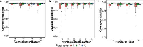
For each simulation dataset, we run 50,000 MCMC iterations with the first 25,000 as burnins. Almost all of the parameters enjoy small biases, standard deviation (SD), and root mean square errors (RMSE), and their coverage probabilities (CP) of the 95% credible interval are high (Figures 1 and Supplement Tables S12–S47).

Fig. 1 Boxplot of coverage probabilities among 100 synthetic replicated datasets (a) when K = 3, $n_{ij}\sim \text{Pois}(25)+5$ and the connectivity probabilities p_c varies over $(0.2,0.3,0.4,0.5)$; (b) when K = 3, $p_c=0.3$, $n_{ij}\sim \text{Pois}(\mu )+5$ and μ varies over $(10,15,20,25,30,35)$; (c) when $p_c=0.3,n_{ij}\sim \text{Pois}(25)+5$ and K varies over $(2,3,4,5)$.

Moreover, these simulation studies allow us to verify the theoretical calculation of time complexity of our MCMC algorithm. Figure 2 confirms that the time complexity of the algorithm is linear in the total number of observed survival times L and quadratic in the number of roles K.

Fig. 2 Running time of 100,000 iterations of the MCMC algorithm on one core of an Intel Xeon Gold 6226R Processor. The number of observations per edge $n_{ij}\sim \text{Pois}(\mu )+5$. (a) We fix the connectivity probability $p_c=0.3$ and μ = 25 while varying the number of roles K from 2 to 5. (b) We fix K = 3 and μ = 25 but vary p_c from 0.2 to 0.5. (c) We fix K = 3 and $p_c=0.3$ but vary μ from 10 to 35.

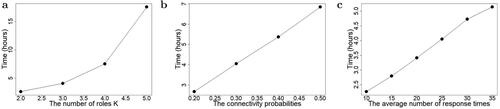
Fig. 3 Patterns learned from the Enron E-mail corpus. (a), (b) The scatterplots of the employee-specific probability ${\pi }_{i1}$ of belonging to the first role and the log-scale E-mail numbers (a) when the SMMB is applied to time-to-event data, and (b) when the MMSB is applied to relational data. Each node represents an employee, with the color indicating his or her position. The size of each node represents the number of E-mails related to the employee. (c) The estimated baseline survival curve $\hspace{0.17em}\exp \hspace{0.17em}\{-\hspace{0.17em}\exp \hspace{0.17em}({\widehat{\beta }}_1^{lk})[1-S_0(t|{\widehat{\mathit{\lambda }}}^{lk})]\}$ of role l replying E-mails to role k when $\mathit{x}={(1,0,0,\dots ,0)}^T$.

We also examine the performance of the conditional DIC in determining the number of roles in the network. For the 100 sets of simulated data with K = 3 roles, $p_c=0.3$ and $n_{ij}\sim \text{Pois}(25)+5$, we run the MCMC algorithm with the number of roles K varying from 2 to 4 for each dataset. It turns out that the conditional DIC correctly identifies the optimal K as three for all of the replicates. Moreover, the conditional DIC also performs well in selecting the optimal number of knots and outperforms the Bayesian information criterion (BIC) (Airoldi et al. 2008) and the Watanabe-Akaike information criterion (WAIC) (Watanabe and Opper 2010) (Supplementary Section S13 and Figures S5–S6).

6 The Enron E-mail Corpus

The Enron E-mail corpus (Klimt and Yang 2004) is the largest publicly available E-mail dataset to date and was released by the Federal Energy Regulatory Commission during its investigation of Enron’s bankruptcy. The dataset contains E-mails generated by 158 Enron employees between November 13, 1998 and June 21, 2002. Because “It’s always about the people. Enron is no different,” (Diesner, Frantz, and Carley 2005) the Enron E-mail corpus provides a unique opportunity to study the communication patterns, company organization, and power spread inside a company. The corpus contains the user information and timestamp of each E-mail. Following the enrondata GitHub repository, we focus on the E-mail folders of 148 Enron users whose positions in the company are known.

We apply the SMMB to the preprocessed dataset (see Supplementary Section S14 for preprocessing details and Table S48). The dataset contains the response times for 25,629 E-mails, 1886 of which are observed and 23,743 are censored. The Kaplan-Meier estimate of the survival probability after three weeks is 92.36%; thus, a cure rate model is necessary to fit the survival function of the response time. We set the number of knots as five and let $(s_0,s_1,s_2,s_3,s_4,s_5)=(0,0.152,0.717,2.83,19.82,504)$ hours such that each interval $(s_{m-1},s_m],m=1,2,3,4,5$ contains the same number of failure times.

6.1 Analysis Without Confidential Information

We first consider the following four covariates: whether the E-mail was sent over the weekend, whether the E-mail was forwarded, the number of recipients of the E-mail, and the number of words in the E-mail. We log-transform the latter two covariates to reduce the impact of skewness. If a series of E-mails had the same subject, we denote the first E-mail as the original E-mail and record the fourth covariate as the number of words in the contents of the original E-mail. The hyperparameters $(a,\kappa ,{\sigma }^2)$ for $(\mathit{\xi },\Lambda ,\mathit{\beta })$ are set as (1, 50, 5). We vary the number of roles K from one to five and run 100,000 MCMC iterations with the first 50,000 iterations as burnins for each value of K. The EPSR values shows that the Markov chain has reached convergence after 50,000 iterations (Supplementary Section S9 and Table S7).

The conditional DIC attains its minimum at K = 2 (Figure S7a), and the SMMB fits the data well (Supplementary Table S11). For K = 2, when we vary the number of knots, the conditional DIC also selects the optimal number of knots as five, thus, M = 5 is a reasonable choice for the data analysis (Figure S7b). In Figure 3(a), we plot the probability ${\pi }_{i1}$ of belonging to the first role as opposed to the second role. Warmer colors (red and deep orange) represent higher positions (CEO and president). The warmer colored points are concentrated on the left-hand side, thus, preferring to belong to the second role, especially the four CEOs shown as red (Table 2). Thus, we regard the second role as the senior group and the first role as the junior group.

Table 2 The estimated role probabilities ${\mathit{\pi }}_i$ by the SMMB from time-to-event data and by the MMSB from binary data of the four CEOs, respectively.

User ID	User Name	SMMB		MMSB
		${\widehat{\pi }}_{i1}$	${\widehat{\pi }}_{i2}$	${\widehat{\pi }}_{i1}$	${\widehat{\pi }}_{i2}$
23	David Delainey	0.049	0.951	0.478	0.522
62	John Lavorato	0.011	0.989	0.835	0.165
63	Kenneth Lay	0.208	0.792	0.463	0.537
117	Jeffrey Skilling	0.014	0.986	0.145	0.855

The estimated baseline survival function of each role pair reveals communication patterns between employees (Figure 3(c)). Let us recall that the role pair (l, k) denotes role k replying to the E-mails from role l. Comparing the survival function of the role pair (1, 2) with that of the other three role pairs, the longest response time was that of a senior employee replying to an E-mail from a junior employee. Meanwhile, the response times between junior employees, which correspond to the role pair (1, 1), were the shortest among all of the role pairs. This may be because junior employees often need to communicate via E-mails about routine daily work. As expected, when a senior employee communicated with a junior employee, which corresponds to the role pairs (1, 2) and (2, 1), junior employees replied to the E-mails from senior employees much faster than the reverse situation. Therefore, the level of seniority affected the speed of E-mail response.

An employee can play different roles when communicating with different colleagues. For example, John Zufferli (User 148) held the position of vice president. When he replied to the E-mails from John Lavorato (User 62), a CEO, the estimated role pair $({\widehat{Q}}_{62,148},{\widehat{R}}_{62,148})=(2,1)$. Meanwhile, when John Lavorato replied to the E-mails from John Zufferli, the estimated role pair became $({\widehat{Q}}_{148,62},{\widehat{R}}_{148,62})=(1,2)$. Thus, John Zufferli occupied a junior position in the communications with the CEO. However, when John Zufferli communicated with Chris Dorland (User 28), a manager, the estimated role pair $({\widehat{Q}}_{148,28},{\widehat{R}}_{148,28})$ and $({\widehat{Q}}_{28,148},{\widehat{R}}_{28,148})$ became (2, 1) and (1, 2), respectively. In other words, compared with Chris Dorland, John Zufferli held a higher position. Thus, although the positions of senders and receivers are not incorporated as covariates, the SMMB is able to reveal the seniority of employees within a company according to E-mail response times.

With regard to the weekend effect (Table 3), among all role pairs, only the 95% credible interval [–5.4631, –0.7872] for the coefficient ${\beta }_2^{11}$ do not cover zero. The negativity of ${\beta }_2^{11}$ indicates that at weekends, junior employees replied to the E-mails sent by other junior employees more slowly, which is unsurprising, as most junior employees are likely to rest over the weekend. The coefficients for the forwarded E-mails are negative across all of the role pairs, indicating that the response times for forwarded E-mails were often longer (Table 3). Moreover, the coefficients for the number of recipients are also negative across role pairs. Thus, an E-mail with more recipients was likely to receive longer response times or was never replied, which is consistent with our experience that people are less likely to respond to circulating E-mails. The effects of E-mail length are only negative for the role pair (1, 1). In other words, for E-mail communications between junior employees, longer E-mails were usually replied to more slowly. The most likely reason for this is that junior employees use E-mails to discuss routine daily work, and a longer E-mail indicates that the task may be more complicated and require more time to handle. Consequently, the SMMB is able to uncover heterogeneous effects across different role pairs.

Table 3 The posterior mean, posterior standard deviation (SD), and 95% credible interval (CI) of coefficient ${\beta }_r^{lk}$’s for the SMMB learned from the Enron E-mail corpus without considering confidential information.

Covariates	Parameters	Posterior mean	Posterior SD	95% CI
Weekend effect	${\beta }_2^{11}$	–2.6923${}^{*}$	1.1340	[–5.4631, –0.7872]
	${\beta }_2^{12}$	–0.9623	1.6866	[–4.6645, 1.6364]
	${\beta }_2^{21}$	0.1191	0.1813	[–0.2510, 0.4611]
	${\beta }_2^{22}$	0.2810	0.2051	[–0.1370, 0.6667]
Forwarded effect	${\beta }_3^{11}$	–1.6664${}^{*}$	0.2363	[–2.1566, –1.2218]
	${\beta }_3^{12}$	–0.9986${}^{*}$	0.5689	[–2.2854, –0.0571]
	${\beta }_3^{21}$	–0.6419${}^{*}$	0.1321	[–0.9028, –0.3852]
	${\beta }_3^{22}$	–0.4578${}^{*}$	0.0960	[–0.6499, –0.2718]
Receiver number	${\beta }_4^{11}$	–1.2633${}^{*}$	0.1600	[–1.5760, –0.9518]
effect	${\beta }_4^{12}$	–1.4220${}^{*}$	0.4894	[–2.4875, –0.5576]
	${\beta }_4^{21}$	–0.7037${}^{*}$	0.0917	[–0.8965, –0.5373]
	${\beta }_4^{22}$	–0.8923${}^{*}$	0.0822	[–1.0588, –0.7376]
Word count effect	${\beta }_5^{11}$	–0.1086${}^{*}$	0.0477	[–0.2033, –0.0140]
	${\beta }_5^{12}$	0.1578	0.1532	[–0.1421, 0.4717]
	${\beta }_5^{21}$	0.0256	0.0399	[–0.0517, 0.1062]
	${\beta }_5^{22}$	–0.0113	0.0334	[–0.0781, 0.0504]

NOTE: The superscript * denotes that the corresponding 95% credible interval does not contain zero.

For comparison, we apply the MMSB (Airoldi et al. 2008) to the binary social network W by running the C# program provided by Burnap et al. (2015). The estimated employee-specific community proportions fail to reflect the leadership among users (Figure 3(b)). For example, the four CEOs had very distinct community proportions (Table 2); therefore, compared with the relational data, the time-to-event data contain much more information about the leadership and power spread of a company. The true position information of these employees shows that the estimated employee-specific role proportions ${\mathit{\pi }}_i,i\in \mathcal{N}$ learned from the response times are much more indicative of the leadership among the employees than those estimated from E-mail counts (Figure 3(a)).

We also apply the expSBM (Rastelli and Fop 2020) by regarding E-mail responses as the interactions in the setting of expSBM. expSBM identifies K = 6 clusters (Table S52). However, the distribution of employees in different groups is very uneven: 127 of 148 employees are clustered into group 2 whereas group 3 contains only one person, the CEO John Lavorato. Moreover, the patterns learned by expSBM fail to characterize the response rates (Tables S53–S54 and Supplementary Section S16).

6.2 Analysis with Confidential Information

Although we usually have no access to E-mail contents or the genders of senders and receivers because of privacy and potential legal issues, we have the unique opportunity to identify each employee and retrieve the E-mail contents for the Enron E-mail corpus. Therefore, we first conduct a sentiment analysis for the E-mail contents. The Loughran and McDonald lexicon (Loughran and McDonald 2011) categorizes words into classes of constraining, litigious, negative, positive, superfluous, and uncertainty (Table S49). For each E-mail, we count the number of words belonging to each category, log-transform them, and add them as six extra covariates to the model. To incorporate gender into the model, we take the male-male actor pair—both the sender and the recipient being male—as the baseline—and create three dummy variables: male–female, female–male, and female–female.

We then refit the SMMB model with 13 covariates. We run 500,000 iterations of the MCMC algorithm, regard the first 250,000 iterations as burnins, and set the variance of the normal prior distribution of $\mathit{\beta }$ as 1. The role proportions (Figure S8) and the baseline survival functions of all role pairs (Figure S9) have similar patterns before and after we incorporate sentiment and gender covariates.

For the four covariates analyzed in Section 6.1, the direction and significance of their effects stay the same in the new analysis except that the 95% credible interval of the weekend effect for the role pair (1, 2), ${\beta }_2^{12}$, no longer covers zero (Table S50). The positivity of ${\beta }_2^{12}$ indicates that at weekends junior employees replied to the E-mails sent by the senior employees even faster. All of the sentiment covariates’ credible intervals cover zero, so they have limited effects on response behavior. Meanwhile, the effects of gender are heterogeneous across different role pairs. As ${\beta }_{12}^{11}$ and ${\beta }_{13}^{11}$ are positive, when two junior employees communicated with each other, they tended to respond faster to E-mails sent by colleagues of the other gender than to those sent by colleagues of the same gender. Moreover, when the sender played a junior role and the receiver played a senior role, male senders were responded faster than female senders as ${\beta }_{12}^{12}$ is significantly greater than 0 but ${\beta }_{13}^{12}$ and ${\beta }_{14}^{12}$ are significantly smaller than 0. In contrast, when senior employees communicated with each other, female senders were responded faster than male senders. Therefore, the analysis with the sentiment and gender covariates again confirms that by allowing different role pairs to have different survival distributions the SMMB model provides novel insights into the company organization.

6.3 Analysis Considering Sending Behavior

To explore whether recent E-mails speed up responses and increase response rates, we introduce a new covariate indicating whether actor i had received an E-mail from actor j within the previous week into the SMMB model in Section 6.1. Table S51 shows that the effects of recent communications are significant and positive for all of the role pairs. However, the patterns of role proportions and baseline survival functions become quite different from those in Section 6.1 (Figures S10–S11). The difference is because the covariate of recent communications encodes information of the frequency of communications, which implies the connectivity of the company but not the leadership relationship. Therefore, to reveal the leadership patterns within the company, we recommend the SMMB model in Section 6.1. Nevertheless, if one is interested in building a prediction model for response times and response rates, we suggest adding covariates related to sending behavior to the SMMB (see Supplementary Section S15 for details).

7 Discussion

In this article, we propose the SMMB to analyze time-to-event data between actor pairs in a social network. In the SMMB, we assume that actor pairs belonging to the same role pairs share the same SCRM, whereas actor pairs belonging to different role pairs have distinct cure rate models. Thus, while keeping the heterogeneity in the response patterns between different role pairs, the SMMB enables us to borrow information across actor pairs for a given role pair. We prove the model identifiability and posterior consistency of the SMMB. We develop an efficient MCMC algorithm for statistical inference.

In our analysis of the Enron E-mail corpus, we did not consider any time-dependent covariates, as they are difficult to construct given the data we have. Nevertheless, for any external time-dependent covariates, we can directly add them into the SMMB (Kalbfleisch and Prentice 2011). In contrast, internal time-dependent covariates may influence the rate of failures, so additional modeling will be needed, which we will investigate in the future.

Thus, far, for a pair of actors, conditional on their roles $(Q_{ij},R_{ij})=(l,k)$, we assume that the sequence of response times is generated independently. When multiple E-mails are about the same topic, there might be dependence between these E-mails. To model dependence, we can further add multiplicative random effects into hazard functions as classic frailty models (Duchateau and Janssen 2008) do (see Supplementary Section S17 for details). As we only have 25,629 E-mails for the Enron E-mail corpus, of which 1886 are observed and the rest are censored, we do not fit these frailty models. Nevertheless, these models might be of interest to large social media and electronic document management systems companies.

With the rapid development of social media and electronic commerce, many social networks now encompass time-to-event data. Although we focus on an E-mail network, many other social networks have similar time-to-event data. For example, the times taken for users to repost messages from other users are available for Twitter. Moreover, in Web-based electronic document management systems such as the services provided by Dropbox and ParaDM, the time that a team member spends on an assigned task can be recorded, and how soon a user responds to the action of another user is also of great interest in this context. We envision that the proposed SMMB can help to analyze these networks and provide insights into information flow, company organization, and working efficiency.

Acknowledgments

We sincerely thank the Editor, Associate Editor, and three reviewers for their helpful comments that have greatly improved the quality of the article.

Disclosure Statement

The authors report there are no competing interests to declare.

Additional information

Funding

The authors gratefully acknowledge the funding support by the Hong Kong PhD Fellowship PF15-17417, GRF 14305318, GRF 14305319, and GRF 14306020 from the Research Grants Council of Hong Kong SAR, China, NSF 2209685 from the National Science Foundation of United States, the Youth Fund No. 12201533 from the National Natural Science Foundation of China, and Shenzhen Stability Support Program from the Shenzhen Science and Technology Innovation Committee.

References

- Airoldi, E. M., Blei, D. M., Fienberg, S. E., and Xing, E. P. (2008), “Mixed Membership Stochastic Blockmodels,” Journal of Machine Learning Research, 9, 1981–2014.
- Burnap, A., Cruz, E., Rong, X., and Segal, B. (2015), “An Implementation of Mixed Membership Stochastic Blockmodel,” available at https://github.com/aburnap/Mixed-Membership-Stochastic-Blockmodel.
- Celeux, G., Forbes, F., Robert, C. P., and Titterington, D. M. (2006), “Deviance Information Criteria for Missing Data Models,” Bayesian Analysis, 1, 651–673. DOI: 10.1214/06-BA122.
- Chen, M.-H., Ibrahim, J. G., and Sinha, D. (1999), “A New Bayesian Model for Survival Data with a Surviving Fraction,” Journal of the American Statistical Association, 94, 909–919. DOI: 10.1080/01621459.1999.10474196.
- Diesner, J., Frantz, T. L., and Carley, K. M. (2005), “Communication Networks from the Enron Email Corpus: It’s Always about the People. Enron is no Different,” Computational & Mathematical Organization Theory, 11, 201–228. DOI: 10.1007/s10588-005-5377-0.
- Duchateau, L., and Janssen, P. (2008), The Frailty Model, New York: Springer.
- Erdős, P., and Rényi, A. (1960), “On the Evolution of Random Graphs,” Mathematical Institute of the Hungarian Academy of Sciences, 5, 17–60.
- Fox, E. W., Short, M. B., Schoenberg, F. P., Coronges, K. D., and Bertozzi, A. L. (2016), “Modeling E-mail Networks and Inferring Leadership using Self-Exciting Point Processes,” Journal of the American Statistical Association, 111, 564–584. DOI: 10.1080/01621459.2015.1135802.
- Gelman, A., Carlin, J. B., Stern, H. S., Dunson, D. B., Vehtari, A., and Rubin, D. B. (2013), Bayesian Data Analysis, Boca Raton,FL: CRC Press.
- Ghosal, S., and Van Der Vaart, A. (2007), “Convergence Rates of Posterior Distributions for Noniid Observations,” The Annals of Statistics, 35, 192–223. DOI: 10.1214/009053606000001172.
- Ghosal, S., and Van der Vaart, A. (2017), Fundamentals of Nonparametric Bayesian Inference (Vol. 44), Cambridge: Cambridge University Press.
- Ibrahim, J. G., Chen, M.-H., and Sinha, D. (2001a), Bayesian Survival Analysis (Vol. 2), New York: Springer.
- Ibrahim, J. G., Chen, M.-H., and Sinha, D. (2001b), “Criterion-based Methods for Bayesian Model Assessment,” Statistica Sinica, 11, 419–443.
- Kalbfleisch, J. D., and Prentice, R. L. (2011), The Statistical Analysis of Failure Time Data, Hoboken: Wiley.
- Kaplan, E. L., and Meier, P. (1958), “Nonparametric Estimation from Incomplete Observations,” Journal of the American Statistical Association, 53, 457–481. DOI: 10.1080/01621459.1958.10501452.
- Kaufmanna, E., Bonaldb, T., and Lelargec, M. (2018), “A Spectral Algorithm with Additive Clustering for the Recovery of Overlapping Communities in Networks,” Theoretical Computer Science, 742, 3–26. DOI: 10.1016/j.tcs.2017.12.028.
- Klimt, B., and Yang, Y. (2004), “The Enron Corpus: A New Dataset for Email Classification Research,” in Machine Learning: ECML 2004, eds. J. F. Boulicaut, F. Esposito, F. Giannotti, and D. Pedreschi, pp. 217–226, Berlin: Springer.
- Liu, J. S. (1994), “The Collapsed Gibbs Sampler in Bayesian Computations with Applications to a Gene Regulation Problem,” Journal of the American Statistical Association, 89, 958–966. DOI: 10.1080/01621459.1994.10476829.
- Loughran, T., and McDonald, B. (2011), “When is a Liability not a Liability? Textual Analysis, Dictionaries, and 10-ks,” The Journal of Finance, 66, 35–65. DOI: 10.1111/j.1540-6261.2010.01625.x.
- Lu, Z., and Song, X. (2012), “Finite Mixture Varying Coefficient Models for Analyzing Longitudinal Heterogenous Data,” Statistics in Medicine, 31, 544–560. DOI: 10.1002/sim.4420.
- Mao, X., Sarkar, P., and Chakrabarti, D. (2017), “On Mixed Memberships and Symmetric Nonnegative Matrix Factorizations,” in International Conference on Machine Learning, pp. 2324–2333.
- Mao, X., Sarkar, P., and Chakrabarti, D. (2021), “Estimating Mixed Memberships with Sharp Eigenvector Deviations,” Journal of the American Statistical Association, 116, 1928–1940. DOI: 10.1080/01621459.2020.1751645.
- Matias, C., Rebafka, T., and Villers, F. (2018), “A Semiparametric Extension of the Stochastic Block Model for Longitudinal Networks,” Biometrika, 105, 665–680. DOI: 10.1093/biomet/asy016.
- Perry, P. O., and Wolfe, P. J. (2013), “Point Process Modelling for Directed Interaction Networks,” Journal of the Royal Statistical Society, Series B, 75, 821–849. DOI: 10.1111/rssb.12013.
- Rastelli, R., and Fop, M. (2020), “A Stochastic Block Model for Interaction Lengths,” Advances in Data Analysis and Classification, 14, 485–512. DOI: 10.1007/s11634-020-00403-w.
- Robbins, H. (1955), An Empirical Bayes Approach to Statistics. Office of Scientific Research, US Air Force.
- Sit, T., Ying, Z., and Yu, Y. (2021), “Event History Analysis of Dynamic Networks,” Biometrika, 108, 223–230. DOI: 10.1093/biomet/asaa045.
- Wang, Y. J., and Wong, G. Y. (1987), “Stochastic Blockmodels for Directed Graphs,” Journal of the American Statistical Association, 82, 8–19. DOI: 10.1080/01621459.1987.10478385.
- Watanabe, S., and Opper, M. (2010), “Asymptotic Equivalence of Bayes Cross Validation and Widely Applicable Information Criterion in Singular Learning Theory,” Journal of Machine Learning Research, 11, 3571–3594.
- Zhang, J., Cai, B., Zhu, X., Wang, H., Xu, G., and Guan, Y. (2022), “Learning Human Activity Patterns Using Clustered Point Processes with Active and Inactive States,” Journal of Business & Economic Statistics, 41, 388–398. DOI: 10.1080/07350015.2021.2025065.
- Zhang, Y., Levina, E., and Zhu, J. (2020), “Detecting Overlapping Communities in Networks Using Spectral Methods,” SIAM Journal on Mathematics of Data Science, 2, 265–283. DOI: 10.1137/19M1272238.