An Automated Approach to Causal Inference in Discrete Settings

Abstract

Applied research conditions often make it impossible to point-identify causal estimands without untenable assumptions. Partial identification—bounds on the range of possible solutions—is a principled alternative, but the difficulty of deriving bounds in idiosyncratic settings has restricted its application. We present a general, automated numerical approach to causal inference in discrete settings. We show causal questions with discrete data reduce to polynomial programming problems, then present an algorithm to automatically bound causal effects using efficient dual relaxation and spatial branch-and-bound techniques. The user declares an estimand, states assumptions, and provides data—however incomplete or mismeasured. The algorithm then searches over admissible data-generating processes and outputs the most precise possible range consistent with available information—that is, sharp bounds—including a point-identified solution if one exists. Because this search can be computationally intensive, our procedure reports and continually refines non-sharp ranges guaranteed to contain the truth at all times, even when the algorithm is not run to completion. Moreover, it offers an ε-sharpness guarantee, characterizing the worst-case looseness of the incomplete bounds. These techniques are implemented in our Python package, autobounds. Analytically validated simulations show the method accommodates classic obstacles—including confounding, selection, measurement error, noncompliance, and nonresponse. Supplementary materials for this article are available online.

KEYWORDS:

• Causal inference
• Constrained optimization
• Partial identification
• Linear programming
• Polynomial programming

1 Introduction

When causal quantities cannot be point identified, researchers often pursue partial identification to quantify the range of possible answers. These solutions are tailored to specific settings (e.g., Lee 2009; Sjölander et al. 2014; Kennedy, Harris, and Keele 2019; Knox, Lowe, and Mummolo 2020; Gabriel, Sachs, and Sjölander 2022), but the idiosyncrasies of applied research can render prior results unusable if even slightly differing scenarios are encountered. This piecemeal approach to deriving causal bounds presents a major obstacle to scientific progress. To increase the pace of discovery, researchers need a more general solution.

In this article, we present an automated approach to causal inference in discrete settings which applies to all causal graphs, as well as all standard observed quantities and domain assumptions. Users declare an estimand, state assumptions, and provide available data—however incomplete or mismeasured. The algorithm numerically computes sharp bounds—the most precise possible answer to the causal query given these inputs, including a unique point estimate if one exists. Our approach accommodates any classic threat to inference—including missing data, selection, measurement error, and noncompliance. It can fuse information from numerous sources—including observational and experimental data, datasets that are unlinkable due to anonymization, or even summary statistics from other studies. The method allows for sensitivity analyses on any assumption by relaxing or removing it entirely. Moreover, it alerts users when assumptions conflict with observed data, indicating faulty causal theory. We also develop techniques for drawing statistical inferences about estimated bounds. We implement these methods in a Python package, autobounds, and demonstrate them with a host of analytically validated simulations.

Our work advances a rich literature on partial identification in causal inference (Manski 1990; Zhang and Rubin 2003; Cai et al. 2008; Swanson et al. 2018; Molinari 2020; Gabriel, Sachs, and Sjölander 2022), outlined in Section 2, which has sometimes cast partial identification as a constrained optimization problem. In pioneering work, Balke and Pearl (1997) provided an automatic sharp bounding method for causal queries that can be expressed as linear programming problems. However, numerous estimands and empirical obstacles do not fit this description, and a complete and feasible computational solution has remained elusive.

When feasible, sharp bounding represents a principled and transparent method that makes maximum use of available data while acknowledging its limitations. Claims outside the bounds can be immediately rejected, and claims inside the bounds must be explicitly justified by additional assumptions or new data. But several obstacles still preclude widespread use. For one, analytic bounds—which can be derived once and then applied repeatedly, unlike our numerical bounds which must be recomputed each time—remain intractable for many problems. Within the subclass of linear problems, Balke and Pearl’s (1997) simplex method offers an efficient analytic approach, but analytic nonlinear solutions are still derived case by case (e.g., Kennedy, Harris, and Keele 2019; Knox, Lowe, and Mummolo 2020; Gabriel, Sachs, and Sjölander 2022). Moreover, though general sharp bounds can in theory be obtained by standard nonlinear optimization techniques (Geiger and Meek 1999; Zhang and Bareinboim 2021), in practice, such approaches are often computationally infeasible. This is because without exhaustively exploring a vast model space to avoid local optima, they can inadvertently report invalid bounds that may fail to contain the truth.

To address these limitations, we first show in Sections 3–4 that—using a generalization of principal strata (Frangakis and Rubin 2002)—causal estimands, modeling assumptions, and observed information can be rewritten as polynomial objective functions and polynomial constraints with no loss of information. We extend results from Geiger and Meek (1999) and Wolfe, Spekkens, and Fritz (2019) to show that essentially all discrete partial identification problems reduce to polynomial programs—a well-studied class of optimization tasks that nest linear programming as a special case.¹ However, it is well known that solving polynomial programs to global optimality is in general NP-hard, highlighting the need for efficient bounding techniques that remain valid even under time constraints (Belotti et al. 2009; Vigerske and Gleixner 2018).

To ameliorate these computational difficulties, Section 4.2 shows how causal graphs can be restated as equivalent canonical models, simplifying the polynomial program. Next, Section 5 develops an efficient optimization procedure, based on dual relaxation and spatial branch-and-bound relaxation techniques, that provides bounds of arbitrary sharpness. We show this procedure is guaranteed to achieve complete sharpness with sufficient computation time; in the problems we examine here, this occurs in a matter of seconds. However, in cases where the time needed is prohibitive, our algorithm is anytime (Dean and Boddy 1988), meaning it can be interrupted to obtain nonsharp bounds that are nonetheless guaranteed to be valid. Crucially, our technique offers an additional guarantee we term “ε-sharpness”—a worst-case looseness factor that quantifies how much the current nonsharp bounds could potentially be improved with additional computation. In Section 6, we provide two approaches for characterizing uncertainty in the estimated bounds. We demonstrate our technique in a series of analytically validated simulations in Section 7, showing the flexibility of our approach and the ease with which assumptions can be modularly imposed or relaxed. Moreover, we demonstrate how it can improve over widely used bounds (Manski 1990) and recover a counterintuitive point-identification result in the literature on nonrandom missingness (Miao et al. 2016).

In short, our approach offers a complete and computationally feasible approach to causal inference in discrete settings. Given a well-defined causal query, valid assumptions, and data, researchers now have a general and automated process to draw causal inferences that are guaranteed to be valid and, with sufficient computation time, provably optimal.

2 Related Literature

Researchers have long sought to automate partial identification by recasting causal bounding problems as constrained optimization problems that can be solved computationally. Our work is most closely related to Balke and Pearl (1997), which showed that certain bounding problems in discrete settings—generally, when interventions and outcomes are fully observed—could be formulated as the minimization and maximization of a linear objective function subject to linear equality and inequality constraints. Such programming problems admit both symbolic solutions and highly efficient numerical solutions. Subsequent studies have proven that the bounds produced by this technique are sharp (Bonet 2001; Ramsahai 2012; Sachs et al. 2022). These results were extended by Geiger and Meek (1999), who showed that a much broader class of discrete problems can be formulated in terms of polynomial relations when analysts have precise information about the kinds of disturbances or confounders that may exist.² In addition to the well-known conditional independence constraints implied by d-separation, these problems imply generalized equality constraints (Verma and Pearl 1990; Tian and Pearl 2002) and generalizations of the instrumental inequality constraints (Pearl 1995; Bonet 2001).

Geiger and Meek (1999) notes that in theory quantifier elimination algorithms can provide symbolic bounds. However, the time required for quantifier elimination grows as a doubly exponential function of the number of parameters, rendering it infeasible for all but the simplest cases. At the core of this issue is that symbolic methods provide a general solution, meaning that they must explore the space of all possible inputs. In contrast, numerical methods such as ours can accelerate computation by eliminating irrelevant portions of the model space.

Even so, computation can be time-consuming.³ In practice, many optimizers can rapidly find reasonably good values but cannot guarantee optimality without exhaustively searching the model space. This approach poses a challenge for obtaining causal bounds, which are global minimum and maximum values of the estimand across all models that are admissible, or consistent with observed data and modeling assumptions. If a local optimizer operates on the original problem (the primal), proceeding from the interior and widening bounds as more extreme models are discovered, then failing to reach global optimality will result in invalid bounds—ranges narrower than the true sharp bounds, failing to contain all possible solutions.

In the following sections, we detail our approach to addressing each of these outstanding obstacles to automating the discovery of sharp bounds for discrete causal problems.

3 Preliminaries

We now define notation and introduce key concepts. A technical glossary is given in Appendix A. We first review how any causal model represented by a directed acyclic graph (DAG) can be “canonicalized,” or reduced into simpler form, without loss of generality (w.l.o.g.; Evans 2016). We describe how these graphs give rise to potential outcomes and a generalization of principal strata (Frangakis and Rubin 2002), two key building blocks in our analytic strategy.

We follow the convention that bold letters denote collections of variables; uppercase and lowercase letters denote random variables and their realizations, respectively. Consider a structured system in which random vectors $\mathit{V}=\{V_1,\dots ,V_J\}$ represent observable main variables and $\mathit{U}=\{U_1,\dots ,U_K\}$ represent unobserved disturbances. We will assume each observed variable V_j is discrete and its space $\mathcal{S}(V_j)$ has finite cardinality; the spaces of unobserved variables are unrestricted. Observed data for each unit $i\in \{1,\dots ,N\}$ is an iid draw from V. Further suppose that causal relationships between all variables in V and U are represented by a nonparametric structural equation model with independent errors (NPSEM-IE; Pearl 2000).⁴ Here, we concentrate on deriving results for the NPSEM-IE model, but our approach is also applicable to the model of Robins (1986) and Richardson and Robins (2013) without change.⁵

Figure 1 presents a DAG $\mathcal{G}$ representing relationships between $\mathit{V}\cup \mathit{U}$. Note that fully observing these variables would be sufficient to identify every quantity we consider in this article. However, since disturbances U are unobserved, and since information about main variables V may be incomplete, partial identification techniques are needed.

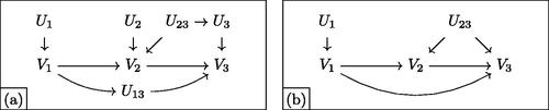
Fig. 1 Canonicalization of a mediation graph. Noncanonical and canonicalized forms are given in panels (a) and (b), respectively. Both are equivalent with respect to their data law. Canonicalization proceeds as follows: (i) the dependent disturbance U₃ is absorbed into its parent U₂₃; (ii) the superfluous U₂ is eliminated as it influences a subset of U₂₃’s children; and (iii) the irrelevant U₁₃ is absorbed into the $V_1\to V_3$ arrow as it is neither observed nor of interest. A complete guide to canonicalization is given in Appendix B.1.

3.1 Canonical DAGs

We now discuss how canonicalizing DAGs—reformulating them w.l.o.g. into a simpler form—simplifies the bounding task. A DAG is said to be in canonical form if (i) no disturbance U_k has a parent in $\mathcal{G}$; and (ii) there exists no pair of disturbances, U_k and $U_{k\prime }$, such that U_k influences a subset of variables influenced by $U_{k\prime }$. Evans (2016) showed that any noncanonical DAG $\mathcal{G}\prime$ has a canonical form $\mathcal{G}$ with an identical distribution governing all variables in V; an algorithm for obtaining this canonical form is given in Appendix B.1. In short, canonicalization distills the data-generating process (DGP) to its simplest form by eliminating potentially complex networks of irrelevant disturbances. Figure 1 shows a noncanonical DAG in panel (a); panel (b) gives the canonicalized version. Note that disturbances affecting only a single variable, such as U₁, are often left implicit; here, we depict them explicitly for clarity.

3.2 Potential Outcomes

The notation of potential outcome functions allows us to compactly express the effects of manipulating variable V_j’s main parents, $\mathit{p}{\mathit{a}}_{\mathit{V}}(V_j)$, or other ancestors that are also main variables. Similarly, $\mathit{p}{\mathit{a}}_{\mathit{U}}(V_j)$ denotes parents of V_j that are disturbances. Let $\mathit{A}\subset \mathit{V}$ be intervention variables that will be fixed to $\mathit{A}=\mathit{a}$. When $\mathit{A}=\varnothing$, so no intervention occurs, then define $V_j(\mathit{a})=V_j$, the natural value. When $\mathit{A}\subseteq \mathit{p}{\mathit{a}}_{\mathit{V}}(V_j)$, so only immediate parents are manipulated, then the potential outcome function is given by its structural equation, $V_j(\mathit{a})=f_j[\mathit{A}=\mathit{a},\mathit{p}{\mathit{a}}_{\mathit{V}}(V_j)\setminus \mathit{A},\mathit{p}{\mathit{a}}_{\mathit{U}}(V_j)]$. For example, in Figure 1(b), the effect of intervention V ₂ = v₂ on outcome V₃ is defined in terms of $V_3(V_2=v_2)=f_3(V_2=v_2,V_1,U_{23})$. Here, the intervention set is $\mathit{A}=V_2$, and the remaining parents of V₃—the non-intervened main parent, $\mathit{p}{\mathit{a}}_{\mathit{V}}(V_3)\setminus \mathit{A}=V_1$, and the disturbance parent, $\mathit{p}{\mathit{a}}_{\mathit{U}}(V_3)=U_{23}$—are allowed to follow their natural distributions. We now define more general potential outcome functions by recursive substitution (Richardson and Robins 2013; Shpitser 2018). For arbitrary interventions on $\mathit{A}\subset \mathit{V}$, let $V_j(\mathit{a})=V_j(\{a_{\mathcal{l}}:{\mathit{A}}_{\mathcal{l}}\in \mathit{p}{\mathit{a}}_{\mathit{V}}(V_j)\}\cup \{V_{j\prime }(\mathit{a}):V_{j\prime }\in \mathit{p}{\mathit{a}}_{\mathit{V}}(V_j)\setminus \mathit{A}\})$; here, $\mathcal{l}$ is a generic index that sweeps over main variables in the graph. That is, if a parent of V_j is in A, it is set to the corresponding value in a. Otherwise, the parent takes its potential value after intervention on causally prior variables, or its natural value otherwise. To obtain the parent’s potential value, apply the same definition recursively.⁶ For example, in Figure 1(b), potential outcomes for V₃ include (i) $V_3(\varnothing )=V_3(V_1,V_2)$, the observed distribution; (ii) $V_3(v_1)=V_3[v_1,V_2(v_1)]$, relating to total effects; and (iii) $V_3(v_1,v_2)$, relating to controlled effects.

3.3 Generalized Principal Stratification

In this section, we show how any DAG and any causal quantity can be represented w.l.o.g. using a generalization of principal strata. Roughly speaking, principal strata on a variable V_j are groups of units that would respond to counterfactual interventions in the same way (Greenland and Robins 1986; Frangakis and Rubin 2002). Formally, let $\mathit{A}=\mathit{p}{\mathit{a}}_V(V_j)$ be an intervention set for which all main parents of V_j are jointly set to some a, and consider unit i’s collection of potential outcomes $\{V_{i,j}(\mathit{A}=\mathit{a}):\mathit{a}\in \mathcal{S}(\mathit{A})\}$. Each principal stratum of V_j then represents a subset of units in which this collection is identical.

The NPSEM of a graph is closely related to its principal stratification. This is because each potential outcome in the collection above is given by $V_{i,j}(\mathit{A}=\mathit{a})=f_j[\mathit{A}=\mathit{a},\mathit{p}{\mathit{a}}_{i,\mathit{U}}(V_j)]$, in which the only source of random variation is unit i’s realization of the relevant disturbances. After fixing these disturbances, all structural equations become deterministic, meaning that a realization of ${\mathit{U}}_i$ must fix every potential outcome for every variable under every intervention. For example, consider the simple DAG $U_1 \to V_1 \to V_2 \leftarrow U_2$, in which V₁ and V₂ are binary. This relationship is governed by the structural equations $V_1=f_1(U_1)$ and $V_2=f_2(V_1,U_2)$, where the functions $f_1:\mathcal{S}(U_1)\to \mathcal{S}(V_1)$ and $f_2:\mathcal{S}(V_1)\times \mathcal{S}(U_2)\to \mathcal{S}(V_2)$ are deterministic and shared across all units. Thus, the only source of randomness is in $\mathit{U}=\{U_1,U_2\}$.

Analysts generally do not have direct information about these disturbances. For example, U₁ could potentially take on any value in $(-\infty ,\infty )$. However, as Proposition 1 will state in greater generality, this variation is irrelevant because V₁ has only two possible values: 0 and 1. The space of U₁ can therefore be divided into two canonical partitions (Balke and Pearl 1997)—those that deterministically lead to $V_1=0$ and those that lead to $V_1=1$—and thus treating U₁ as if it were binary is w.l.o.g.

Strata for V₂ are similar but more involved. After U₂ is realized, it induces the partially applied response function $V_2=f_2(V_1,U_2=u_2)=f_2^{(u_2)}(V_1)$, which deterministically governs how V₂ counterfactually responds to V₁. Regardless of how many are in $\mathcal{S}(U_2)$, this response function must fall into one of only four possible strata, each a mapping of the form $f_2^{(u_2)}:\mathcal{S}(V_1)\to \mathcal{S}(V_2)$ (Angrist, Imbens, and Rubin 1996). These groups are (i) $V_2=1$ regardless of V₁, “always takers” or “always recover”; (ii) $V_2=0$ regardless of V₁, “never takers” or “never recover”; (iii) $V_2=V_1$, “compliers,” or those “helped” by V₁; and (iv) $V_2=1-V_1$, “defiers,” or those “hurt” by V₁. Thus, from the perspective of V₂, any finer-grained variation in $\mathcal{S}(U_2)$ beyond the canonical partitions is irrelevant. These partitions are in one-to-one correspondence with principal strata, which in turn allow causal quantities to be expressed in simple algebraic expressions. For example, the average treatment effect (ATE) is equal to the proportion of compliers minus that of defiers.⁷ As Proposition 2 will show, by writing down all information in terms of these strata, essentially any causal inference problem can be converted into an equivalent optimization problem involving polynomials of variables that represent strata sizes.

Finally, consider the more complex mediation DAG of Figure 2(a). Response functions for V₁ and V₂ remain as above. In contrast, V₃ is caused by $\mathit{p}{\mathit{a}}_{\mathit{V}}(V_3)=\{V_1,V_2\}$ via the structural equation $V_3=f_3(V_1,V_2,U_{23})$. Substituting in disturbance $U_{23}=u_{23}$ produces one of 16 response functions of the form $f_3^{(u_{23})}:\mathcal{S}(V_1)\times \mathcal{S}(V_2)\to \mathcal{S}(V_3)$, yielding 16 strata.⁸

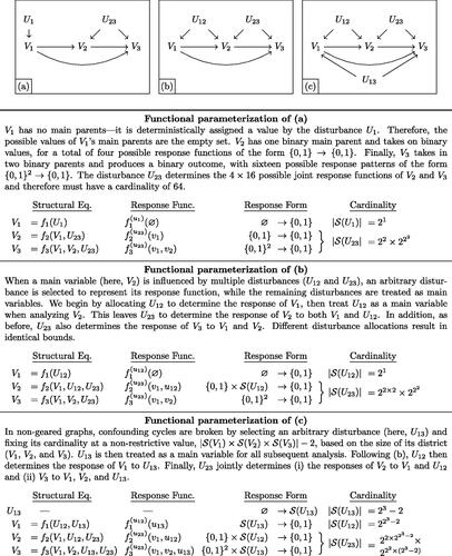
Fig. 2 Any discrete-variable DAG can be represented in terms of generalized principal strata. Panels (a–b) depict geared graphs. In (a), each main variable is influenced by only one disturbance. In (b), V₂ is influenced by both U₁₂ and U₂₃. In (c), a nongeared graph with cyclical confounding by U₁₂, U₂₃, and U₁₃ is shown. For each case, the functional parameterizations—representations of each graph in terms of generalized principal strata—are illustrated.

In turn, the number of principal strata determines the minimum complexity of a reduced but nonrestrictive alternative model in which the full data law, or joint distribution over every potential outcome, is preserved. This means the reduction is w.l.o.g. for every possible factual or counterfactual quantity involving V. Specifically, the number of principal strata in the graph determines the minimum cardinalities of each $U_k\in \mathit{U}$ that are needed to represent the original model w.l.o.g., if we were to redefine U_k in terms of a categorical distribution over principal strata. For example, to capture the joint response patterns that a unit may have on V₂ and V₃, a reduced version of U₂₃ can express any full data law if it has a cardinality of $|\mathcal{S}(U_{23})|=4\times 16$, because V₂ has four possible response functions and V₃ has 16.

Below, Proposition 1 states that a generalization of this approach can produce nonrestrictive models w.l.o.g. for any discrete-variable DAG and any full data law. Crucially, this also holds for (i) graphs where a variable V_j is influenced by multiple disturbances U_k and $U_{k\prime }$, as in Figure 2(b); and (ii) the challenging case of nongeared graphs (Evans 2018) such as Figure 2(c)—roughly speaking, when disturbances U_k, $U_{k\prime }$, and $U_{k″}$ touch overlapping combinations of main variables to create cycles of confounding. Formalization is provided later.

Proposition 1.

Suppose $\mathcal{G}$ is a canonical DAG over discrete main variables V and disturbances U with infinite cardinality. The model over the full data law implied by $\mathcal{G}$ is unchanged by assuming that the disturbances have sufficiently large finite cardinalities.

A proof can be found in Appendix F.1, along with details on how to obtain a lower bound on nonrestrictive cardinalities for the disturbances. Briefly, Proposition 1 extends a result from Finkelstein, Wolfe, and Shpitser (2021), which showed there are reductions of $\mathcal{S}(\mathit{U})$ that do not restrict the model over the factual V. We build on this result to show that there are reductions that do not restrict the full data law—that is, the model over all factual and counterfactual versions of V.

Though the theory of principal stratification is well understood when each main variable V_j is influenced by only one disturbance U_k, complications arise when V_j is influenced by multiple disturbances U_k and $U_{k\prime }$. For each such main variable, any one of the associated disturbances can be allocated to take primary responsibility—that is, to be the input for which the response function is partially applied. For the purposes of defining this response function, all remaining disturbances are treated as if they were main variables.⁹ For example, in Figure 2(b), V₂ is influenced by both U₁₂ and U₂₃; we will allocate V₂ to U₂₃ for illustration, but allocating it to U₁₂ would produce identical bounds. Next, we compute the cardinality of remaining disturbances as usual. Here, U₁₂ is left only to determine V₁, meaning that it has a cardinality of two. Finally, we return to the primary disturbance and determine its cardinality based on main variables and remaining disturbances. In this example, after fixing U₂₃, the variable V₂ is a function of V₁ and U₁₂, both binary, meaning that U₂₃ has a cardinality of sixteen.

Finally, Proposition 1 extends Evans (2018) by allowing us to develop generalized principal strata for graphs that are nongeared, meaning that disturbances do not satisfy the running intersection property.¹⁰ These cases differ only in that they contain cycles of confounding; after breaking the cycle at any point, they can be dealt with in the same manner as geared graphs. An example of a nongeared graph is given in Figure 2(c). Finkelstein, Wolfe, and Shpitser (2021) presents an algorithm for constructing a generalized principal stratification for nongeared graphs. In brief, the algorithm breaks the confounding cycle by selecting an arbitrary disturbance—for example, U₁₃—and fixing its cardinality at a value that is guaranteed to be nonrestrictive of the model over factual random variables, by Carathéodory’s theorem. In this case, based on U₁₃’s district,¹¹ $\{V_1$, V₂, $V_3\}$, U₁₃ can be analyzed w.l.o.g. as if it had a cardinality of $|\mathcal{S}(V_1)\times \mathcal{S}(V_2)\times \mathcal{S}(V_3)|-2$. In all subsequent analysis of Figure 2(c), U₁₃ would then be treated as a main variable, allowing the graph to be analyzed as if it were geared. As in Figure 2(b), U₁₂ then determines the response of V₁ to U₁₃. Finally, U₂₃ jointly determines (i) the responses of V₂ to V₁ and U₁₂ as well as (ii) V₃ to V₁, V₂, and U₁₃. We note that the number of parameters involved in nongeared graphs can quickly become intractable. In these cases, valid but possibly nonsharp bounds can always be obtained by solving a relaxed problem in which a single disturbance is connected to each main variable in a district, absorbing multiple disturbances that influence only a subset of those variables (for example, adding a U₁₂₃ that absorbs U₁₂, U₁₃, and U₂₃).

In sum, all classes of discrete-variable DAGs can be parameterized in terms of generalized principal strata. In what follows, we show how this representation allows us to reformulate causal bounding problems in terms of polynomial programs that can be optimized over the sizes of these strata, subject to constraints implied by assumptions and available data.

4 Formulating the Polynomial Program

We now turn to the central problem of this article: sharply bounding causal quantities with incomplete information. Our approach is to transform the task into a constrained optimization problem that can be solved computationally by (i) rewriting the causal estimand into a polynomial expression, and (ii) rewriting modeling assumptions and empirical information into polynomial constraints. Appendix C.1 provides a detailed walkthrough of this process with a concrete instrumental variable problem, along with example code that illustrates how the above steps are automated by our software in merely eight lines of code.

Our goal is to obtain sharp bounds on the estimand, or the narrowest range that contains all admissible values consistent with available information: structural causal knowledge in the form of a canonical DAG, $\mathcal{G}$; empirical evidence, $\mathcal{E}$; and modeling assumptions, $\mathcal{A}$, formalized below. Importantly, our definition of “empirical evidence” flexibly accommodates essentially any data about the joint, marginal, or conditional distributions of the main variables.

We will suppose the main variables take on values in a known, discrete set, $\mathcal{S}=\mathcal{S}(\mathit{V})$. In this section, we will demonstrate (i) that $\{\mathcal{G},\mathcal{E},\mathcal{A},\mathcal{S}\}$ restricts the admissible values of the target quantity, and (ii) this range of observationally indistinguishable values can be recovered by polynomial programming. The causal graph and variable space, $\mathcal{G}$ and $\mathcal{S}$, together imply an infinite set of possible structural equation models, each capable of producing the same full data laws. By Proposition 1, w.l.o.g., we can consider a simple model in which (i) each counterfactual main variable is a deterministic function of exogeneous, discrete disturbances; (ii) there are a relatively small number of such disturbances; and (iii) disturbances take on a finite number of possible values, corresponding to principal strata of the main variables. When repeatedly sampling units (along with each unit’s random disturbances, U), the kth disturbance thus follows the categorical distribution with parameters ${\mathcal{P}}_{U_k}=\{\text{Pr}(U_k=u_k):u_k\in \mathcal{S}(U_k)\}$. By the properties of canonical DAGs, these disturbances are independent. It follows that the parameters ${\mathcal{P}}_{\mathit{U}}$ of the joint disturbance distribution $\text{Pr}(\mathit{U}=\mathit{U})=\prod _k\text{Pr}(U_k=u_k)$ not only fully determine the distribution of each factual main variable under no intervention, $V_j(\varnothing )$—they also determine the counterfactual distribution of $V_j(\mathit{a})$ under any intervention a, as well as its joint distribution with other counterfactual variables $V_{j\prime }(\mathit{a}\prime )$ under possibly different interventions $\mathit{a}\prime$. This leads to the following proposition, proven in Appendix F.2.

Proposition 2.

Suppose $\mathcal{G}$ is a canonical DAG and $C_{\mathcal{l}}:\mathcal{l}$ is a set of counterfactual statements, indexed by $\mathcal{l}$, in which ${\mathcal{C}}_{\mathcal{l}}=\{V_{\mathcal{l}}({\mathit{a}}_{\mathcal{l}})=v_{\mathcal{l}}\}$ states that variable $V_{\mathcal{l}}$ will take on value $v_{\mathcal{l}}$ under manipulation ${\mathit{a}}_{\mathcal{l}}$. Let $\mathbb{1}\{\mathit{U}\Rightarrow \{{\mathcal{C}}_{\mathcal{l}}:\mathcal{l}\left\}\right\}$ be an indicator function that evaluates to 1 if and only if disturbance realizations $\mathit{U}=\{u_1,\dots ,u_K\}$ deterministically lead to ${\mathcal{C}}_{\mathcal{l}}$ being satisfied for every $\mathcal{l}$. Then under the structural equation model for $\mathcal{G}$, $$\text{Pr}\left(\underset{\mathcal{l}}{\cap }{\mathcal{C}}_{\mathcal{l}}\right)=\sum _{\mathit{U}\in \mathcal{S}(\mathit{U})}\mathbb{1}\{\mathit{U}\Rightarrow \{{\mathcal{C}}_{\mathcal{l}}:\mathcal{l}\left\}\right\}\prod _{u_k\in \mathit{U}}\text{Pr}(U_k=u_k),$$which is a polynomial equation in ${\mathcal{P}}_{\mathit{U}}$, the probabilities $\text{Pr}(U_k=u_k)$.

For example, in the mediation setting of Figure 1(b), Proposition 2 implies that the joint distribution of the factual variables—$V_1(\varnothing ),V_2(\varnothing )$, and $V_3(\varnothing )$—is given by $$\begin{array}{c}\text{Pr}(V_1(\varnothing )=v_1,V_2(\varnothing )=v_2,V_3(\varnothing )=v_3)\\ \mathrm{\hspace{1em}}\mathrm{\hspace{1em}}=\sum _{\{u_1,u_{23}\}\in \mathcal{U}}\text{Pr}(U_1=u_1)\text{Pr}(U_{23}=u_{23}),\end{array}$$where $\mathcal{U}=\{\mathit{U}:\mathit{U}\Rightarrow \mathit{V}\}$ is the set of disturbance realizations that are consistent with a particular $\mathit{V}(\varnothing )=\mathit{V}$. In other words, $$\mathcal{U}=\left\{\{u_1,u_{23}\}:f_1^{(u_1)}(\varnothing )=v_1,f_2^{(u_{23})}(v_1)=v_2,f_3^{(u_{23})}(v_1,v_2)=v_3\right\}.$$

Alternatively, analysts may be interested in the probability that a randomly drawn unit i has a positive controlled direct effect when fixing the mediator to $V_2 = 0$. This is given by $\text{Pr}[V_3(V_1 = 0,V_2 = 0) = 0,V_3(V_1 = 1,V_2 = 0) = 1]$ and is similarly expressed in terms of the disturbances as $\sum _{\{u_1,u_{23}\}\in \mathcal{U}\prime }\text{Pr}(U_1 = u_1)\text{Pr}(U_{23} = u_{23})$, summing over a different subset of the disturbance space, $\mathcal{U}\prime = \left\{\right\{u_1,u_{23}\}:$ $f_3^{(u_{23})}(V_1 = 0,V_2 = 0) = 0,f_3^{(u_{23})}(V_1 = 1,V_2 = 0) = 1\}$.

We now expand this result to include a large class of functionals of marginal probabilities and logical statements about these functionals.

Corollary 1.

Suppose $\mathcal{G}$ is a canonical DAG. Let ${\mathcal{P}}_{\mathit{V}}$ denote the full data law and $g_1({\mathcal{P}}_{\mathit{V}})$ denote a functional of ${\mathcal{P}}_{\mathit{V}}$ involving elementary arithmetic operations on constants and marginal probabilities of ${\mathcal{P}}_{\mathit{V}}$. Then $g_1({\mathcal{P}}_{\mathit{V}})$ can be re-expressed as a polynomial fraction in the parameters of ${\mathcal{P}}_{\mathit{U}},g_2({\mathcal{P}}_{\mathit{U}})$, by replacing each marginal probability with its Proposition 2 polynomialization.

We denote this replacement process with the operation $\mathit{polynomial}-\mathit{fractionalize}\left[{\mathrm{g}}_1({\mathcal{P}}_{\mathit{V}})\right]$. The corollary has a number of implications, which we discuss briefly. First, it shows that a wide array of single-world and cross-world functionals can be expressed as polynomial fractions. These include traditional quantities such as the ATE, as well as more complex ones such as the pure direct effect and the probability of causal sufficiency. It also suggests any nonelementary functional of ${\mathcal{P}}_{\mathit{V}}$ can be approximated to arbitrary precision by a polynomial fraction, if the functional has a convergent power series. We note that nonelementary functionals rarely arise in practice, apart from logarithmic- or exponential-scale estimands.¹² An example that our approach cannot handle is the nonanalytic functional $\mathbb{1}\left\{\text{ATE is rational}\right\}$.

A nonobvious implication of Corollary 1 is that when (i) $g_1({\mathcal{P}}_{\mathit{V}})$ is an elementary arithmetical functional; (ii) $★\in \{<,\le ,=,\ge ,>\}$ is a binary comparison operator; and (iii) α is a finite constant, then any statement of the form $g_1({\mathcal{P}}_{\mathit{V}}) ★ \alpha$ can be transformed into a set of equivalent non-fractional relations, $\{h_{\mathcal{l}}({\mathcal{P}}_{\mathit{U}},\mathit{s}) {\star }_{\mathcal{l}} 0:\mathcal{l}\}$. Here, each $h_{\mathcal{l}}(·)$ denotes a non-fractional polynomial in the parameters indicated; ${\star }_{\mathcal{l}}$ is a possibly different binary comparison from $★$; and s are newly created auxiliary variables that are sometimes necessary. The transformation proceeds as follows. First, $g_1({\mathcal{P}}_{\mathit{V}}) ★ \alpha$ can be rewritten as $g_2({\mathcal{P}}_{\mathit{U}}) ★ \alpha$, by Proposition 1. Then, note that any fractional $g_2({\mathcal{P}}_{\mathit{U}})$ can be rewritten as some $\frac{g_3({\mathcal{P}}_{\mathit{U}})}{h({\mathcal{P}}_{\mathit{U}})}$ in which $g_3({\mathcal{P}}_{\mathit{U}})$ has fewer fractions than $g_2({\mathcal{P}}_{\mathit{U}})$. Regardless of whether $h({\mathcal{P}}_{\mathit{U}})$ is positive, negative, or of indeterminate sign, it can be shown that $h({\mathcal{P}}_{\mathit{U}})$ can be cleared to obtain an equivalent relation. The exact procedure differs for each case and, when $h({\mathcal{P}}_{\mathit{U}})$ is indeterminate, requires a set of auxiliary variables, s, to be created.¹³ If all fractions have been cleared from $g_3({\mathcal{P}}_{\mathit{U}})$, then the rewritten statement is also of the promised form and we are done; otherwise, recurse. We denote this transformation of the original statement—that is, polynomial-fractionalizing its components and then clearing all resulting fractions—as $\mathit{polynomialize}\left[{\mathrm{g}}_1({\mathcal{P}}_{\mathit{V}}) ★ \alpha \right]$.

By the same token, any estimand $g_1({\mathcal{P}}_{\mathit{V}})$ that is a polynomial-fractional $g_2({\mathcal{P}}_{\mathit{U}})$ in the parameters of ${\mathcal{P}}_{\mathit{U}}$ can be re-expressed as a polynomial in the expanded parameter space, $h({\mathcal{P}}_{\mathit{U}},\mathit{s})$, along with a set of additional polynomial relations. To see this, first define a new estimand, s, which is a monomial (and hence a polynomial). This new estimand can be made equivalent to the original one by imposing a new polynomial-fractional constraint, $s-g_2({\mathcal{P}}_{\mathit{U}})=0$. Any remaining fractions in the new constraint are cleared as above. We will make extensive use of these properties to convert causal queries to polynomial programs.

Algorithm 2 in the supplementary materials provides a step-by-step procedure for formulating a polynomial programming problem. Solving this program via Algorithm 3 in the supplementary materials then produces sharp bounds. Both algorithms, given in Appendix B, mirror the discussion here with more formality. We begin by transforming a factual or counterfactual target of inference $\mathcal{T}$ into polynomial form, possibly creating additional auxiliary variables to eliminate fractions. To accomplish this task, the procedure uses the possibly noncanonical DAG $\mathcal{G}$ and the variable space $\mathcal{S}(\mathit{V})$ to re-express $\mathcal{T}$ in terms of functional parameters that correspond to principal strata proportions. The result is the objective function of the polynomial program. The procedure then polynomializes the sets of constraints resulting from empirical evidence and by modeling assumptions, respectively denoted $\mathcal{E}$ and $\mathcal{A}$. In Figure 2, if only observational data is available, then $\mathcal{E}$ consists of eight pieces of evidence, each represented as a statement corresponding to a cell of the factual distribution $\text{Pr}[V_1(\varnothing )=v_1,V_2(\varnothing )=v_2,V_3(\varnothing )=v_3]=\text{Pr}(V_1=v_1,V_2=v_2,V_3=v_3)$ for observable values in ${\{0,1\}}^3$. Modeling assumptions include all other information, such as monotonicity or dose-response assumptions; these can be expressed in terms of principal strata. For example, the assumed unit-level monotonicity of the $V_1\to V_2$ relationship (e.g., the “no defiers” assumption of Angrist, Imbens, and Rubin 1996) can be written as the statement that $\text{Pr}(V_2(V_1=0)=1,V_2(V_1=1)=0)=0$.¹⁴ Finally, the statement that each disturbance U_k follows a categorical probability distribution is re-expressed as the polynomial relations $\text{Pr}(U_k=u_k)\ge 0\forall u_k$ and $\sum _{u_k}\text{Pr}(U_k=u_k)=1$.

Algorithm 2 produces an optimization problem with a polynomial objective subject to polynomial constraints. This polynomial programming problem is equivalent to the original causal bounding problem. This leads directly to the following theorem.

Theorem 1.

Minimization (maximization) of the polynomial program produced by Algorithm 2 produces sharp lower (upper) bounds on $\mathcal{T}$ under the sample space $\mathcal{S}(\mathit{V})$, structural equation model $\mathcal{G}$, additional modeling assumptions $\mathcal{A}$, and empirical evidence $\mathcal{E}$.

4.1 Example Program for Outcome-based Selection

For intuition, consider the simple example in Figure 3, motivated by a hypothetical study of discrimination in traffic law enforcement using (a) police data on vehicle stops and (b) traffic-sensor data on overall vehicle volume. For illustrative purposes, suppose all drivers behave identically. Here, $X\in \{0,1\}$ indicates whether a motorist is a racial minority and $Y\in \{0,1\}$ whether the motorist is stopped by police. X and Y are assumed to be unconfounded. However, there exists outcome-based selection: we only learn driver race (X) from police records if a stop occurs (Y = 1), precluding point identification. Panels (a–d) in Figure 3 depict the inputs to the algorithm: (a) the causal graph, $\mathcal{G}$; (b) the observed evidence, $\mathcal{E}$, consisting of the marginal $\text{Pr}(Y=y)$ and the conditional $\text{Pr}(X=x|Y=1)$; (c) additional assumptions, $\mathcal{A}$, the monotonicity assumption that white drivers are not discriminatorily stopped; and (d) the sample space $\mathcal{S}(X,Y)$. The target $\mathcal{T}$ is the ATE, $\mathbb{E}[Y(X=1)-Y(X=0)]$, the amount of anti-minority bias in stopping. Next, Figure 3(e) depicts functional parameterization in terms of six disturbance partitions, following Section 3.3. Applying simplifications from Section 4.2 results in elimination of $\text{Pr}(\text{Y-defier})$ by assumption, then elimination of redundant strata that complete the sum to unity, $\text{Pr}(\text{X-control})$ and $\text{Pr}(\text{Y-never})$. The problem can thus be reduced to three dimensions. Next, the ATE is rewritten as the probability of an anti-minority stop, minus that of an anti-white stop (which is zero by assumption). Finally, Figure 3(f–i) depict how each constraint narrows the space of potential solutions, leaving the admissible region shown in Figure 3(i)—the only part of the model space simultaneously satisfying all constraints.

Fig. 3 Visualization of Algorithm 2. Constructing the polynomial program for a simple bounding problem with outcome-dependent selection, motivated by a study of discrimination in traffic law enforcement. Panels (a)–(d) depict inputs to the algorithm. The graph, $\mathcal{G}$, contains unconfounded treatment X and outcome Y. The evidence $\mathcal{E}$ contains (i) the marginal distribution of Y and (ii) the conditional distribution of X if Y = 1. $\mathcal{A}$ consists of a monotonicity assumption. $\mathcal{S}$ states that X and Y are binary. The target $\mathcal{T}$ is the ATE $\mathbb{E}[Y(x=1)-Y(x=0)]$. Panel (e) depicts functional parameterization with six disturbance partitions, following Section 3.3. Applying simplifications from Section 4.2 results in elimination of $\text{Pr}(\text{Y-defier})$ by assumption, then elimination of $\text{Pr}(\text{X-control})$ and $\text{Pr}(\text{Y-never})$ by the second axiom. Panels (f)–(i) show constraints in the simplified model space.

Once formulated in this way, optimization proceeds by locating the highest and lowest values of $\mathcal{T}$ within this region, which respectively represent the upper and lower bounds on the ATE. A variety of computational solvers can in principle be used to minimize and maximize it.¹⁵ However, in practice, the resulting polynomial programming problem can be much more complex than the simple case shown in Figure 3. For example, even seemingly simple causal problems can result in nonconvex objective functions or constraints; moreover, both the admissible region of the model space and the region of possible objective values can be disconnected.¹⁶ Local solvers thus cannot guarantee valid bounds without exhaustively searching the space; when time is finite, these can fail to discover global extrema for the causal estimand, resulting in invalid intervals that are not guaranteed to contain the quantity of interest.

4.2 Simplifying the Polynomial Program

The time needed to solve polynomial programs can grow exponentially with the number of variables. To address this, in Appendix D, we employ various techniques that draw on graph theory and probability theory to simplify polynomial programs into forms with fewer variables that generally have identical solutions but are usually faster to solve. At a high level, these simplifications fall into four categories. First, Appendix D.1 proposes a simplification that reduces the degree of polynomial expressions. Using the graph’s structure, we show how to detect when a disturbance Uk is guaranteed to be irrelevant, meaning its parameters only occur in contexts where $\sum _{u_k\in \mathcal{S}(U_k)}\text{Pr}(U_k=u_k)$ can be factored out and replaced with unity. Second, Appendix D.2 introduces a simplification that reduces the degree of polynomial expressions by exploiting equality constraints like the simple $\text{Pr}(\text{X-control})+\text{Pr}(\text{X-treated})=1$ example above. We note some practical considerations when using symbolic algebra systems such as SageMath (Stein et al. 2019), specifically about the computational efficiency of factoring out complex polynomial expressions and replacing them with constants, as opposed to solving for one variable in terms of others. Third, Appendix D.3 discusses a broad class of simplifications that reduce the number of constraints in the program, but with important tradeoffs. We show that assumptions encoded in a DAG, such as the empty binary graph $U_X\to X\mathrm{\hspace{1em}}\mathrm{\hspace{1em}}Y\leftarrow U_Y$, allow the empirical evidence to be expressed using fewer constraints—here, the reduction uses only two pieces of information, $\text{Pr}(X=1)$ and $\text{Pr}(Y=1)$, exploiting the previously mentioned equality constraints and the assumed independence of X and Y. This is a reduction from the three pieces of information needed to convey $\text{Pr}(X=x,Y=y)$,¹⁷ but comes at the cost that analysts can no longer falsify the independence assumption. Finally, Appendix D.4 provides a simplification for detecting when constraints and parameters no longer bind the objective function, meaning they can be safely eliminated from the program.

We caution that the practical application of these techniques remains an important area for future research: applying these techniques in different orders, or even with slightly different software implementations, can produce optimization programs that are mathematically equivalent but can vary substantially in runtime.

5 Computing ε-sharp Bounds in Polynomial Programs

We now turn to the practical optimization of the polynomial program defined by Algorithm 2, which we refer to as the primal program. Per Theorem 1, minimization and maximization of the polynomialized target, $\mathcal{T}(\mathit{p})$, is equivalent to the causal bounding problem. (Optimization is implicitly over the admissible region of the model space.) We denote the sharp lower and upper bounds as $\underset{¯}{T}\equiv {\min }_{\mathit{p}}\mathcal{T}(\mathit{p})$ and $\overline{T}\equiv {\max }_{\mathit{p}}\mathcal{T}(\mathit{p})$. As we note above, the challenge is that these problems are often nonconvex and high dimensional, meaning globally optimal solutions can be difficult to obtain. Conventional primal optimizers, which iteratively improve suboptimal values, can be trapped in local extrema, resulting in invalid bounds that fail to contain all possible values of the estimand (including global extrema).

To address this challenge and guarantee the validity of reported bounds, our approach incorporates dual techniques that do not directly optimize the original primal objective function, $\mathcal{T}(\mathit{p})$. Instead, these techniques construct alternative objective functions that are easier to optimize; solutions to the easier dual problems can then be related back to the original primal problems. In particular, we will construct piecewise linear dual envelope functions $\underset{¯}{\mathcal{D}}(\mathit{p})$ and $\overline{\mathcal{D}}(\mathit{p})$ that satisfy $\underset{¯}{\mathcal{D}}(\mathit{p})\le \mathcal{T}(\mathit{p})\le \overline{\mathcal{D}}(\mathit{p})$ for all p in the admissible region. An illustration is given in Figure 4(b). In statistics, related techniques have found use in variational inference—an approach that constructs an analytically tractable dual function that can be maximized in place of the likelihood function (Jordan et al. 1999; Blei, Kucukelbir, and McAuliffe 2017).¹⁸

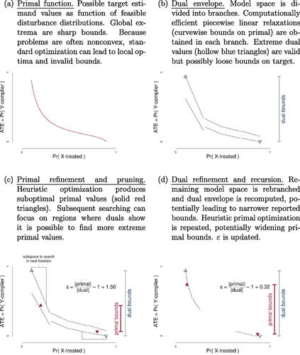
Fig. 4 Visualization of Algorithm 3. Computing ε-sharp bounds for the outcome-based selection problem of Figure 3. Panel (a) shows how the target ATE varies over the feasible region of the model space (reparameterized in terms of possible ${\mathcal{P}}_{\mathit{U}}$ distributions) depicted in Figure 3(i). Panel (b) depicts the first step of our method, partitioning of the model space into branches within which computationally tractable, piecewise linear dual relaxations are obtained. Panel (c) shows how suboptimal values of the primal function, obtained with standard local optimizers, can be combined with the dual envelope to prune large regions of the model space that cannot possibly contain the global extrema. In panel (d), the procedure is applied recursively. The pruned model space is rebranched and heuristic primal optimization is repeated, potentially yielding narrower dual bounds and wider primal bounds, respectively. The looseness factor, ε, narrows until reaching zero (sharpness) or a specified threshold.

A key property of this envelope is that the easier-to-compute dual bounds, $\underset{¯}{D}\equiv {\min }_{\mathit{p}}\underset{¯}{\mathcal{D}}(\mathit{p})$ and $\overline{D}\equiv {\max }_{\mathit{p}}\overline{\mathcal{D}}(\mathit{p})$, will always bracket the unknown true sharp bounds. This is because $\underset{¯}{\mathcal{D}}(\mathit{p})$ and $\overline{\mathcal{D}}(\mathit{p})$ are downward- and upward-shifted relaxations of the original objective function, which can only lead to a lower minimum and higher maximum, respectively. The dual bounds are thus guaranteed to be valid causal bounds. Viewed differently, the dual bounds $\left[\underset{¯}{D},\overline{D}\right]$ also represent outer bounds (where bounding addresses the computationally difficult task of computing the global extrema) on the unknown sharp causal bounds $\left[\underset{¯}{T},\overline{T}\right]$ (where bounding addresses the fundamental unknowability of the DGP). Here, a key consideration is that the choice of a dual envelope determines the looseness, or the duality gaps $\underset{¯}{T}-\underset{¯}{D}$ and $\overline{D}-\overline{T}$. Our task therefore reduces to the question of how to evaluate the looseness of the dual bounds and, if needed, to refine the envelope so that it leads to tighter dual bounds.

We now discuss our procedure for assessing the looseness of the dual bounds. To start, note that for any admissible point in the model space, p, the corresponding value of the target quantity, $\mathcal{T}(\mathit{p})$, must satisfy $\underset{¯}{T}\le \mathcal{T}(\mathit{p})\le \overline{T}$ by definition, even when the true sharp bounds are unknown. This immediately suggests that for any collection of points $\{\mathit{p},\mathit{p}\prime ,\mathit{p}″,\dots \}$ within the admissible region where we choose to evaluate $\mathcal{T}(·)$, the lowest and highest values discovered—which we denote $\underset{¯}{P}$ and $\overline{P}$—must also be contained within the sharp bounds. In other words, $\left[\underset{¯}{P},\overline{P}\right]$ represents an inner bound on the unknown sharp bounds $\left[\underset{¯}{T},\overline{T}\right]$. Therefore, for any choice of dual envelope and any collection of evaluated points, we have $\underset{¯}{D}\le \underset{¯}{T}\le \underset{¯}{P}\le \overline{P}\le \overline{T}\le \overline{D}$. We evaluate the looseness of the reported dual bounds by taking the ratio of the outer bounds’ excess width to the width of the inner bounds, $\epsilon \equiv (\overline{D}-\underset{¯}{D})/(\overline{P}-\underset{¯}{P})-1$. It can be seen that when $\underset{¯}{P}=\underset{¯}{D}$ and $\overline{P}=\overline{D}$, then the reported dual bounds have provably attained sharpness and $\epsilon =0$. However, $\epsilon >0$ does not necessarily imply that the dual bounds are not sharp; for example, it may simply be that $\underset{¯}{D}=\underset{¯}{T}$, so the lower bound is sharp, but the collection of points evaluated is insufficiently large, so that $\underset{¯}{T}<\underset{¯}{P}$ and this sharpness cannot be proven. For this reason, we refer to ε as the worst-case looseness factor.

We are now ready to discuss how bounds are iteratively refined; a step-by-step procedure is given in Algorithm 3 in Appendix B. Note that at the outset of the procedure, the initial dual envelope may lie far from the true objective function, meaning ε will be large. We employ the spatial branch-and-bound approach to recursively subdivide the model space and efficiently search for regions in which the bounds may be improved. A variety of mature optimization frameworks can be used to implement the proposed methods, including Couenne and SCIP (Belotti et al. 2009; Vigerske and Gleixner 2018); the key to Algorithm 3 is that the upper- and lower-bounding optimization problems must be executed in parallel, so that the relative looseness ε can be tracked over time. In addition to the polynomial program produced by Algorithm 2, our procedure accepts two stopping parameters: ${\epsilon }^{\text{thresh}}$, the desired level of provable sharpness; and ${\theta }^{\text{thresh}}$, an acceptable width for the bounds width $\theta \equiv \overline{D}-\underset{¯}{D}$.¹⁹

Figure 4 illustrates the procedure for the outcome-based selection problem of Figure 3. The algorithm receives the primal objective function, $\mathcal{T}(\mathit{p})$, shown in Figure 4(a), as input. It then partitions the parameter space into a series of branches, or connected subsets of the parameter space. Separate partitions, $\underset{¯}{\mathcal{B}}$ and $\overline{\mathcal{B}}$, are used for lower and upper bounding, respectively. Within each branch b, a linear function ${\mathcal{D}}_b(\mathit{p})$ is constructed; easily computed properties such as derivatives and boundary values are used to ensure that this plane lies above or below $\mathcal{T}(\mathit{p})$ for all admissible points in the branch.²⁰ We collect these branch-specific bounds in the piecewise functions $\underset{¯}{\mathcal{D}}(\mathit{p})\equiv \left\{{\underset{¯}{\mathcal{D}}}_b(\mathit{p})\text{ if }\mathit{p}\in {\underset{¯}{\mathcal{B}}}_b:b\right\}$ and $\overline{\mathcal{D}}(\mathit{p})\equiv \left\{{\overline{\mathcal{D}}}_b(\mathit{p})\text{ if }\mathit{p}\in {\overline{\mathcal{B}}}_b:b\right\}$, which define the initial dual envelope shown with dashed blue lines in Figure 4(b). Because each piece is linear, it is straightforward to compute the extreme points of the dual envelope within each branch, ${\underset{¯}{D}}_b=\min \left\{{\underset{¯}{\mathcal{D}}}_b(\mathit{p}):\mathit{p}\in {\underset{¯}{\mathcal{B}}}_b\right\}$ and ${\overline{D}}_b=\max \left\{{\overline{\mathcal{D}}}_b(\mathit{p}):\mathit{p}\in {\overline{\mathcal{B}}}_b\right\}$. The overall dual (outer) bounds are then $\underset{¯}{D}={\min }_b{\underset{¯}{D}}_b$ and $\overline{D}={\max }_b{\overline{D}}_b$, depicted with hollow blue triangles.

Next, the algorithm seeks to expand the primal (inner) bounds. Recall that these bounds, $[\underset{¯}{P},\overline{P}]$, are the minimum and maximum values of the target function that have been encountered in any set of admissible DGPs—regardless of how that set was constructed. We can therefore use standard constrained optimization techniques to optimize the primal problem. Various heuristics—for example, initializing optimizers in regions that appear promising based on the duals—can also be used. The fact that these techniques are only guaranteed to produce local optima is not of concern, because primal bounds are used only for computational convenience. Examples of two admissible primal points are shown with red triangles in Figure 4(c). These primal bounds represent the narrowest possible causal bounds: the (unknown) sharp lower bound $\underset{¯}{T}$ must satisfy $\underset{¯}{T}\le \underset{¯}{P}$, and similarly the sharp upper bound must satisfy $\overline{P}\le \overline{T}$. This means entire swaths of the parameter space can now be ignored, greatly accelerating the search. For example, in Figure 4(c), the upper dual function (upper dashed blue lines) indicates that the rightmost three-quarters of the parameter space cannot possibly produce a target value that is higher than $\overline{P}$—the upper primal bound that has already been found (upper solid red triangle). Therefore, optimization of the upper dual bound can focus on the bracketed “subspace to search in next iteration.” Optimization of the lower dual bound only need consider regions that $\underset{¯}{\mathcal{D}}(\mathit{p})$ indicates can produce lower values than $\underset{¯}{P}$.

A new, refined dual envelope can now be constructed by subdividing the remaining space and recomputing tighter dual functions, as shown in Figure 4(d). The procedure is then repeated recursively—the algorithm heuristically selects branches in the model space that appear promising, then refines primal and dual bounds in turn. If a more extreme admissible target value is found, it is stored as a new primal bound. Finally, the algorithm prunes branches of $\underset{¯}{\mathcal{B}}$ and $\overline{\mathcal{B}}$ that cannot improve dual bounds or that wholly violate constraints. Optimization terminates when either ε reaches ${\epsilon }^{\text{thresh}}$ or θ reaches ${\theta }^{\text{thresh}}$. For complex problems, the time to convergence may be prohibitive. But because the dual function is always guaranteed to contain the true objective function, the algorithm is anytime—the user can halt the program at any point and obtain valid (but potentially loose) bounds.

6 Statistical Inference

We now, briefly discuss how to modify Algorithm 3 to account for sampling error in the empirical evidence used to construct bounds. A more rigorous formalization is provided in Appendix E.

Consider a simulated binary $X\to Y$ graph with confounding $X\leftarrow U_{XY}\to Y$. Up until now, when discussing how empirical evidence constrains the admissible DGPs, we have only considered population distributions of observable quantities—here, $\mathcal{E}=\{\text{Pr}(X=0,Y=0)=0.121,\text{Pr}(X=1,Y=0)=0.346,\text{Pr}(X=0,Y=1)=0.349,\text{Pr}(X=1,Y=1)=0.184\}$. When these population constraints are input to the algorithm, we refer to the results as the population bounds. In practice, however, analysts only have access to noisily estimated versions; with N = 1000, the sample analogues might respectively be 0.113, 0.352, 0.357, and 0.178. By the plug-in principle, estimated bounds are obtained by supplying estimated constraints instead. In other words, we apply the algorithm as if $\text{Pr}(X=x,Y=y)=\widehat{\text{Pr}}(X=x,Y=y)$.

Next, we propose two easily polynomializable methods to account for uncertainty from sampling error. Our general approach is to relax empirical-evidence constraints: we say that $\text{Pr}(X=x,Y=y)$ must be near $\widehat{\text{Pr}}(X=x,Y=y)$, rather than equaling it. Our first method is based on the “Bernoulli-KL” approach of Malloy, Tripathy, and Nowak (2020), which constructs separate confidence regions for each observable $\text{Pr}(X=x,Y=y)$. For example, rather than constraining Algorithm 3 to only consider DGPs exactly satisfying $\text{Pr}(X=0,Y=0)=0.121$, as in the population bounds, or $\text{Pr}(X=0,Y=0)=0.113$, as in the estimated bounds, we instead allow it to consider any DGP in which $0.073\le \text{Pr}(X=0,Y=0)\le 0.163$. Thus, each equality constraint in the original empirical evidence is replaced with two linear inequality constraints; this is equivalent to constraining $\text{Pr}(X=x,Y=y)$ to lie within a hypercube.

Our second method is based on the multivariate Gaussian limiting distribution of the multinomial proportion (Bienaymé 1838). This approach will essentially say that $\text{Pr}(X=x,Y=y)$ is constrained to lie within an ellipsoid, rather than a hypercube. Let $\widehat{\mathit{E}}$ be a vector collecting $[\widehat{\text{Pr}}(X=0,Y=0)$, $\widehat{\text{Pr}}(X=1,Y=0),\widehat{\text{Pr}}(X=0,Y=1)]$.²¹ We then compute a confidence region for the distribution $\mathcal{N}(\widehat{\mathit{E}},\frac{1}{N}\text{diag}(\widehat{\mathit{E}})-\frac{1}{N}\widehat{\mathit{E}}{\widehat{\mathit{E}}}^{\top })$. This replaces all of the original equality constraints with a single quadratic inequality constraint of the form ${(\widehat{\mathit{E}}-\mathit{E})}^{\top }{(\frac{1}{N}\text{diag}(\widehat{\mathit{E}})-\frac{1}{N}\widehat{\mathit{E}}{\widehat{\mathit{E}}}^{\top })}^{-1}(\widehat{\mathit{E}}-\mathit{E})\le z$, where $\mathit{E}=[\text{Pr}(X=0,Y=0)$, $\text{Pr}(X=1,Y=0),\text{Pr}(X=0,Y=1)]$ and z is some critical value of the ${\chi }^2$ distribution.

Specifics of the calculations are given in Appendix E. These confidence regions for the empirical quantities aim to jointly cover $\text{Pr}(X=x,Y=y)$, for every x and y, in at least $1-\alpha$ of repeated samples (the Bernoulli-KL method guarantees conservative coverage in finite samples, whereas the Gaussian method offers only asymptotic guarantees). When this holds, confidence bounds obtained by optimizing subject to the relaxed empirical constraints are guaranteed to have at least $1-\alpha$ coverage of the population bounds. In Section 7.2, we show that empirically, confidence bounds obtained from both methods are conservative.

7 Simulated Examples

7.1 Instrumental Variables

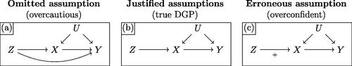
Noncompliance with randomized treatment assignment is a common obstacle to causal inference. Balke and Pearl (1997) showed that bounds on the ATE under noncompliance can be obtained via linear programming. However, that approach cannot be used to bound the local ATE (LATE) among “compliers” because this quantity is nonlinear. Angrist, Imbens, and Rubin (1996) shows the LATE can be point identified if certain conditions hold—including, notably, (i) the absence of a direct effect of treatment assignment Z on the outcome Y; and (ii) monotonicity, or the absence of “defiers” in which actual treatment X is the inverse of Z.²² Because these may not be satisfied in practice, Figure 5 shows three possible sets of assumptions that analysts may make: (a) neither; (b) the former but not the latter; and (c) both. We simulate a true DGP corresponding to panel (b), in which no-direct-effect holds but monotonicity is violated. The true ATE is –0.25 and the true LATE is –0.36. We will suppose analysts have access to the population distribution $\text{Pr}(Z=z,X=x,Y=y)$; inference is discussed in Section 7.2.

Fig. 5 DGPs with noncompliance. Three possible scenarios involving encouragement Z, treatment X, and outcome Y. Panel (b) represents the true simulation DGP, where $Z\to X$ monotonicity is violated (indicated by absence of a +). Panel (a) depicts assumptions used by an “overcautious” analyst unwilling to assume away a direct $Z\to Y$ effect. Panel (c) corresponds to an “overconfident” analyst that incorrectly assumes monotonicity of $Z\to X$.

An overcautious analyst might be unwilling to rule out a direct $Z\to Y$ effect or defiers in $Z\to X$, making only assumptions shown in panel (a). Applying our method yields bounds of $[-0.63,0.37]$ and $[-1,1]$ for the ATE and LATE, respectively—sharp, but uninformative in sign. With an additional no-direct-effect assumption, per panel (b), they would instead obtain ATE bounds of $[-0.55,-0.15]$, revealing a negative effect and correctly containing the true ATE, –0.25. However, LATE bounds remain at $[-1,1]$; as compliers cannot be identified experimentally, this quantity is difficult to learn about without strong assumptions. Finally, an overconfident analyst might mistakenly make an additional monotonicity assumption. Helpfully, when asked to produce bounds, Algorithm 3 reports the causal query is infeasible—meaning that it cannot locate any DGP consistent with data and assumptions. This clearly warns that the causal theory is deficient. If the analyst naïvely applied the traditional two-stage least-squares estimator, they would receive no such warning. Instead, they would obtain an erroneous point estimate of –0.74, roughly double the true LATE of –0.36.

7.2 Coverage of Confidence Bounds

We now evaluate the performance of confidence bounds that characterize uncertainty due to sampling error, constructed according to Section 6 and Appendix E, using the instrumental variable model of Figure 5(b). Specifically, we draw samples of N = 1000, $N=10,000$, or $N=100,000$ observations from this DGP. For each sample, we then use the empirical proportions $\frac{1}{N}\sum _i\mathbb{1}\{Z_i=z,X_i=x,Y_i=y\}$ for all $x,y,z\in \{0,1\}$. These eight quantities form the basis of estimated bounds, by the plug-in principle. To quantify uncertainty, we compute 95% confidence regions on the same observed quantities, then convert them to polynomial constraints for inclusion in Algorithm 3. Optimizing subject to these confidence constraints produces confidence bounds, depicted in Figure 6. For each combination of sample size and uncertainty method, we draw 1000 simulated datasets and run Algorithm 3 on each.

Fig. 6 Coverage of confidence bounds. Each of 1000 simulations is depicted with a horizontal line. For each simulation, a horizontal error bar represents estimated bounds (top panels) or 95% confidence bounds (middle and lower panels), obtained per Section 6. All confidence bounds fully contain the population bounds, indicating 100% coverage. The middle (lower) row of panels reflect confidence bounds obtained with the Bernoulli-KL (asymptotic) method. Columns of panels report confidence bounds obtained using samples of various sizes. Vertical dotted gray lines show true population lower and upper bounds, which contain the true ATE of –0.25; vertical dashed black lines indicate zero.

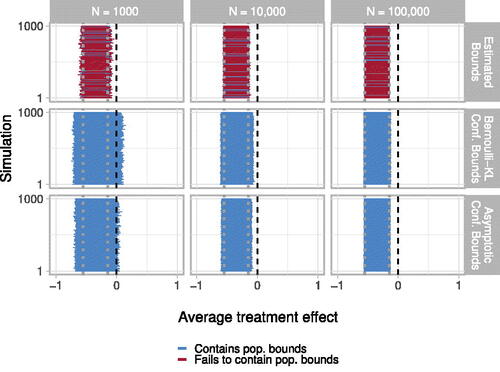
Table 1 reports average values of estimated confidence bounds obtained by Algorithm 3 over 1000 simulated datasets, for varying N. At all sample sizes, estimated bounds are centered on population bounds. Figure 13 in the supplementary materials shows confidence bounds obtained across methods and sample sizes. The Bernoulli-KL method produces wider confidence intervals at all N; at N = 1000, it is generally unable to reject zero, whereas the asymptotic method does so occasionally. Differences in interval width persist but shrink rapidly as sample size grows and both methods collapse on population bounds. As discussed in Section 6, we find more conservative coverage for confidence bounds on the ATE (100% coverage of population bounds), compared to coverage of the underlying confidence regions on the observed quantities (95% joint coverage of observed population quantities for the asymptotic method).

Table 1 Bias of estimated bounds. Average estimated upper and lower bounds, across 1000 simulated datasets, for varying sample sizes. Estimated bounds are centered on population bounds in all scenarios.

Quantity	N = 1000	$N=10,000$	$N=100,000$	Population
Lower bound	−0.5497	−0.5498	−0.5500	−0.5502
Upper bound	−0.1453	−0.1455	−0.1459	−0.1460

7.3 More Complex Bounding Problems

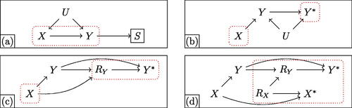
We now examine four hypothetical DGPs, shown in Figure 7, featuring various threats to inference. Throughout, we target the ATE of X on Y. Panel (a) illustrates outcome-based selection: we observe unit i only if S_i = 1, where S_i may be affected by Y. Selection severity, $\text{Pr}(S=0)$, is known, but no information about $\text{Pr}(X=x,Y=y|S=0)$ is available. X and Y are also confounded by unobserved U. Bounding in this setting is a nonlinear program, with an analytic solution recently derived in Gabriel, Sachs, and Sjölander (2022). Panel (b) illustrates measurement error: an unobserved confounder U jointly causes Y and its proxy $Y^{\ast }$, but only treatment and the proxy outcome are observed. Bounding in this setting is a linear problem. A number of results for linear measurement error were recently presented in Finkelstein et al. (2020); here, we examine the monotonic errors case, where $Y^{\ast }(Y=1)\ge Y^{\ast }(Y=0)$. Panel (c) depicts missingness in outcomes, that is, nonresponse or attrition. Here, X affects both the partially observed Y and response indicator R; if R = 1, then $Y^{\ast }=Y$, but if R = 0, then $Y^{\ast }$ takes on the missing value indicator NA. Nonresponse on Y is differentially affected by both X and the value of Y itself (i.e., “missingness not at random,” MNAR); Manski (1990) provides analytic bounds. Finally, panel (d) depicts joint missingness in both treatment and outcome—sometimes a challenge in longitudinal studies with dropout—with MNAR on Y.

Fig. 7 Various threats to inference. Panels depict (a) outcome-based selection, (b) measurement error, (c) nonresponse, and (d) joint missingness. In each graph, X and Y are treatment and outcome, respectively. Dotted red regions represent observed information. In (a), the box around S indicates selection: other variables are only observed conditional on S = 1. In (b), $Y^{\ast }$ represents a mismeasured version of the unobserved true Y. In (c), R_Y indicates reporting, so that $Y^{\ast }=Y$ if R = 1 and is missing otherwise. In (d), both treatment and outcome can be missing, and missingness on X can affect missingness on Y.

Figure 8 illustrates how Algorithm 3 recovers sharp bounds. Each panel shows progress in time. Primal bounds (blue) can widen over time if more extreme, observationally equivalent models are found. Dual bounds (red) narrow as the outer envelope is tightened. Our method simultaneously searches for more extreme primal points and narrows the dual envelope. Analysts can terminate the process at any time, reporting guaranteed-valid dual bounds along with their worst-case suboptimality factor, ε—or await complete sharpness, $\epsilon =0$.

Fig. 8 Computation of ATE bounds. Progress of Algorithm 3 for simulation data from DGPs depicted in Figure 7(a)–(d). Black error bars are known analytic bounds, y-axes are ATE values, and x-axes are runtimes of Algorithm 3. Red regions are dual bounds, which always contain sharp bounds and the unknown true causal effect; these can only narrow over time, converging on optimality. Blue regions are primal bounds, which can only widen over time as more extreme models are found. Optimization stops when primal and dual bounds meet, indicating bounds are sharp. Prior analytic bounds are sharp for problems (a)–(c). In setting (d), Algorithm 3 achieves point identification, but Manski (1990) bounds do not.

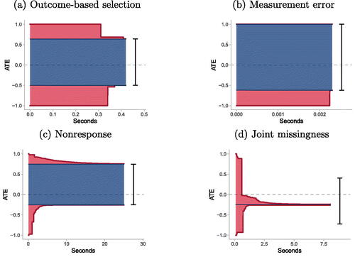
In Figure 8(a)–(c), the algorithm converges on known analytic results. Ultimately, in the selection simulation (a), Algorithm 3 achieves bounds of $[-0.50,0.64]$, correctly recovering Gabriel, Sachs, and Sjölander’s (2022) analytic bounds; in (b), measurement error bounds are $[-0.62,1.00]$, matching Finkelstein et al. (2020); and in (c), outcome missingness bounds are $[-0.25,0.75]$, equaling Manski (1990) bounds. Somewhat counterintuitively, Figure 8(d) shows dual bounds collapsing to a point, eventually point-identifying the ATE at –0.25 despite severe missingness. This surprising result turns out to be a variant of an approach using “shadow variables” developed by Miao et al. (2016).²³ This example illustrates the algorithm is general enough to recover results even when they are not widely known in a particular model; note the commonly used approach of Manski (1990) produces far looser bounds of $[-0.72,0.40]$, failing to exploit causal structure given in Figure 7(d). This result suggests our approach enables an empirical investigation of complex models where general identification results are not yet available. Situations where bounds converge suggest models where point identification via an explicit functional may be possible, potentially enabling new identification theory.

8 Potential Critiques of the Approach

Below, we briefly discuss several potential critiques of our method.

“The user must know the true causal model.” This is false; users do not need to assert an incorrect “complete” model, but rather only what they know or believe. Our approach simply derives the conclusions that follow from data and those transparently stated assumptions.

“The bounds will be too wide to be informative.” This is no tradeoff: faulty point estimates based on faulty assumptions are also uninformative. When sharp bounds incorporating all defensible assumptions are wide, it merely means progress will require more information.

“What about continuous variables?” Discrete approximations often suffice in applied work. If continuous treatments only affect discrete outcomes when exceeding a threshold, discretization is lossless. Future work may study discrete approximations when effects are smooth.

“The bounds will take too long to compute.” Achieving $\epsilon =0$ may sometimes take prohibitive time, but our approach remains faster than manual derivation. Figure 8 shows that several recently published results were recovered in mere seconds. Moreover, our anytime guarantee ensures that premature termination will still produce valid bounds.

9 Conclusion

Causal inference is a central goal of science, and many established techniques can point-identify causal quantities under ideal conditions. But in many applications, these conditions are simply not satisfied, necessitating partial identification—yet few tools for obtaining these bounds exist. For knowledge accumulation to proceed in the messy world of applied statistics, a general solution is needed. We present a tool to automatically produce sharp bounds on causal quantities in settings involving discrete data. Our approach involves a reduction of all such causal queries to polynomial programming problems, enables efficient search over observationally indistinguishable DGPs, and produces sharp bounds on arbitrary causal estimands. This approach is sufficiently general to accommodate essentially every classic inferential obstacle.

Beyond providing a general tool for causal inference, our approach aligns closely with recent calls to improve research transparency by explicitly declaring estimands, identifying assumptions, and causal theory (Miguel et al. 2014; Lundberg, Johnson, and Stewart 2021). Only with a common understanding of goals and premises can scholars have meaningful debates over the credibility of research. When aspects of a theory are contested, our approach allows for a fully modular exploration of how assumptions affect empirical conclusions. Scholars can learn whether assumptions are empirically consequential, and if so, craft a targeted line of inquiry to probe their validity. Our approach can also act as a safeguard for analysts, flagging assumptions as infeasible when they conflict with observed information.

Key avenues for future research are uncertainty quantification and computation time for complex problems. While we develop conservative confidence bounds and anytime validity guarantees, future work should pursue confidence bounds with nominal coverage and computational improvements, perhaps by incorporating point-identified subquantities or semi-parametric modeling. Causal inference scholars may also use this method to aid in the exploration of new identification theory. These lines of inquiry now represent the major open questions in discrete causal inference.

Supplementary Materials

Appendices include (a) a technical glossary; (b) detailed algorithms; (c) worked examples; (d) details on program simplifications; (e) details on statistical inference; (f) proofs; and (g) details of simulations. Our replication archive consists of a Docker container including code, a snapshot of our autobounds package, and all dependencies needed to reproduce reported results.

Acknowledgments

For helpful feedback, we thank Peter Aronow, Justin Grimmer, Kosuke Imai, Luke Keele, Gary King, Christopher Lucas, Fredrik Sävje, Brandon Stewart, Eric Tchetgen Tchetgen, and participants in the Harvard Applied Statistics Workshop, the New York University Data Science Seminar, University of Pennsylvania Causal Inference Seminar, PolMeth 2021, and the Yale Quantitative Research Methods Workshop.

Disclosure Statement

The authors report there are no competing interests to declare.

Additional information

Funding

We gratefully acknowledge financial support from AI for Business and the Analytics at Wharton Data Science and Business Analytics Fund, the Carnegie Corporation of New York, the Office of Naval Research under grant N00014-21-1-2820, the National Science Foundation under grants 2040804 and CAREER 1942239, and the National Institutes of Health under grant R01 AI127271-01A1. The statements made and views expressed are solely the responsibility of the authors.

Notes

1 Specifically, our results apply to elementary arithmetic functionals or monotonic transformations thereof—a broad set that essentially includes all causal assumptions, observed quantities, and estimands in standard use. For example, the average treatment effect and the log odds ratio can be sharply bounded with our approach, but nonanalytic functionals (which are rarely if ever encountered) cannot. Functionals that do not meet these conditions can be approximated to arbitrary precision, if they have convergent power series.

2 A subtle point in nonlinear settings is that the region of possible values for the estimand—that is, estimand values associated with models in the model subspace that are consistent with available data and assumptions—may be disconnected. That is, while the sharp lower and upper bounds correspond to minimum and maximum possible values of the estimand, not all estimand values between these extremes are necessarily possible.

3 Sharp bounds can always be obtained by exhaustively searching the model space. But the computation time required to do so—that is, to solve the polynomial programming problem—can explode with the number of variables (principal strata sizes).

4 The NPSEM-IE model states that each $V_j\in \mathit{V}$ and each $U_k\in \mathit{U}$ is a deterministic function of (i) variables in $\mathit{V}\cup \mathit{U}$ corresponding to its parents in $\mathcal{G}$ and (ii) an additional disturbance term, ${ϵ}_{V_j}$ or ${ϵ}_{U_k}$. The crucial assumption in the NPSEM-IE is that these ϵ terms are mutually independent. Note that throughout this article, we keep the presence of ϵ variables implicit; we will prove that each V_j can equivalently viewed as a deterministic function of its parents in $\mathit{V}\cup \mathit{U}$, absorbing the variation induced by ϵ terms into U.

5 See Appendix F.3 for further discussion of the finest fully randomized causally interpretable structured tree graph (FFRCISTG; described in Richardson and Robins 2013).

6 When defining potential outcomes for V_j, intervention on V_j itself is ignored.

7 To see this, note that the ATE is given by $\mathbb{E}[V_2(V_1=1)-V_2(V_1=0)]=\sum _{\text{strata}}\mathbb{E}[V_2(V_1=1)-V_2(V_1=0)|\text{strata}]·\text{Pr}(\text{strata})=0·\text{Pr}(\text{always taker})+0·\text{Pr}(\text{never taker})+1·\text{Pr}(\text{complier})-1·\text{Pr}(\text{defier})$.

8 More generally, the number of unique response functions grows with (i) the cardinality of the variable, (ii) the number of causal parents it has, and (iii) the parents’ cardinalities. Specifically, V_j has $|\mathcal{S}(V_j){|}^{|\mathcal{S}(\mathit{p}{\mathit{a}}_{\mathit{V}}(V_j))|}$ possible mappings: given a particular input from V_j’s parents, the number of possible outputs for V_j is $|\mathcal{S}(V_j)|$; the number of possible inputs from V_j’s parents is $|\mathcal{S}(\mathit{p}{\mathit{a}}_{\mathit{V}}(V_j))|=\prod _{V_{j\prime }\in \mathit{p}{\mathit{a}}_{\mathit{V}}(V_j)}|\mathcal{S}(V_{j\prime })|$, the product of the parents’ cardinalities.

9 Note that if any main variable V has multiple parents in U, there may be multiple valid parameterizations—that is, methods for constructing generalized principal strata—depending on which disturbance is assigned primary responsibility for determining which main variable. If each main variable has only a single parent in U, there is only a single functional parameterization.

10 Here, the running intersection property requires that there exists a total ordering of disturbances such that any set of main variables that are children of a disturbance U_k, as well as disturbances earlier in the ordering than U_k, must all be children of a specific disturbance earlier in the ordering than U_k. For example, in Figure 2(c), if the ordering is $U_{13}<U_{12}<U_{23}$, then V₂ and V₃ are both children of U₂₃ and earlier disturbances; thus, both must be simultaneously influenced by at least one of the earlier disturbances. This is not the case, and furthermore, there exists no other ordering that satisfies the requirement, so Figure 2(c) is nongeared. For further discussion, see Finkelstein, Wolfe, and Shpitser (2021)

11 Districts of a canonical graph are components that remain connected after removing arrows among V.

12 Bounds on a monotonic transform of x can be obtained by bounding x, then applying the transform.

13 First, consider strictly positive $h({\mathcal{P}}_{\mathit{U}})$; here, $g_3({\mathcal{P}}_{\mathit{U}})-\alpha h({\mathcal{P}}_{\mathit{U}}) ★ 0$ is equivalent to the original statement. Second, consider strictly negative $h({\mathcal{P}}_{\mathit{U}})$: clearing the fraction yields $g_3({\mathcal{P}}_{\mathit{U}})-\alpha h({\mathcal{P}}_{\mathit{U}}) \star 0$, where $\star$ reverses an inequality $★$. Finally, in the case when $h({\mathcal{P}}_{\mathit{U}})$ can take on both positive and negative values, let an auxiliary variable $s\in \mathit{s}$ be defined such that $s·h({\mathcal{P}}_{\mathit{U}})-1=0$, which is a polynomial relation of the promised form. It can now be seen that the original statement is equivalent to $s·g_3({\mathcal{P}}_{\mathit{U}})-\alpha ★ 0$. For a concrete example of how auxiliary variables can be used to clear fractions, see Appendix C.1.3.

14 Assumed population-level monotonicity is typically written $\mathbb{E}[V_2(V_1=1)-V_2(V_1=0)]\ge 0$, but can be rewritten in terms of strata as $\text{Pr}[V_2(V_1=1)=1,V_2(V_1=0)=0]-\text{Pr}[V_2(V_1=0)=1,V_2(V_1=1)=0]\ge 0$.

15 Throughout this article, we will neglect the distinction between minimum (maximum) and infimum (supremum), as is standard practice in numerical optimization.

16 For example, the polynomial constraint $x^3-x^2\le -0.1$ would produce a disconnected admissible region of $x\in (-\infty ,-0.280]\cup [0.413,0.867]$. Moreover, even connected admissible regions can produce disconnected sets of possible objective values; for example, with the objective $\frac{1}{x}$ (which can be transformed to a polynomial objective, as discussed on page 7), the constraint $\{-1\le x\le 1\}$ leads to possible objective values of $(-\infty ,-1]\cup [1,\infty )$. Note that discontinuity is merely a computational challenge rather than a conceptual issue, as the definition of the bounds in this case would be $\left[{\min }_{x\in [-1,1]}\frac{1}{x},{\max }_{x\in [-1,1]}\frac{1}{x}\right]=(-\infty ,\infty )$.

17 Any one of the four cells can be automatically eliminated, as it is redundant given the implied constraint that $\sum _{x,y}\text{Pr}(X=x,Y=y)=1$ by construction of the principal strata.

18 Variational inference uses an analytic relaxation to obtain a single dual function that lower-bounds the likelihood function everywhere in the model space. Our approach diverges in that (i) we conduct two simultaneous dual relaxations to obtain an envelope—both lower and upper—for the original primal function; (ii) we computationally generate piecewise dual functions, rather than analytically deriving smooth duals, and (iii) instead of working with a fixed dual function, we generate a sequence of dual envelopes that iteratively tighten the duals.

19 We include ${\theta }^{\text{thresh}}$ to address the possibility of point identification, in which case $\overline{P}-\underset{¯}{P}=0$, finite ${\epsilon }^{\text{thresh}}$ cannot be achieved, and algorithms based on this stopping criteria alone will not terminate.

20 For example, consider the objective function $\mathcal{T}(x)=x^2$. Any tangent line is a valid lower dual function. Moreover, within any interval $[x_a,x_b]$, the secant line from $(x_a,\mathcal{T}(x_a))$ to $(x_b,\mathcal{T}(x_b))$ is a valid upper dual function. A piecewise linear envelope can thus be constructed by proceeding one branch at a time, computing derivatives (for example, at the branch midpoint) to obtain a branch-specific lower dual function ${\underset{¯}{\mathcal{D}}}_b(x)$ and boundary values to obtain a branch-specific upper dual function ${\overline{\mathcal{D}}}_b(x)$.

21 To avoid degeneracy issues, one empirical quantity is excluded, as it must sum to unity.

22 Other conditions include ignorability of Z and a nonnull effect of Z on X.

23 Specifically, it can be shown the ATE is identified for the Figure 7(d) graph only among faithful distributions where $X\to Y$ is nonnull—that is, almost everywhere in the model space.

References

- Angrist, J. D., Imbens, G. W., and Rubin, D. B. (1996), “Identification of Causal Effects Using Instrumental Variables,” Journal of the American Statistical Association, 91, 444–455. DOI: 10.1080/01621459.1996.10476902.
- Balke, A., and Pearl, J. (1997), “Bounds on Treatment Effects from Studies with Imperfect Compliance,” Journal of the American Statistical Association, 92, 1171–1176. DOI: 10.1080/01621459.1997.10474074.
- Belotti, P., Lee, J., Liberti, L., Margot, F., and Wächter, A. (2009), “Branching and Bounds Tightening Techniques for Non-convex MINLP,” Optimization Methods and Software, 24, 597–634. DOI: 10.1080/10556780903087124.
- Bienaymé, I. J. (1838), Mémoire sur la probabilité des résultats moyens des observations: démonstration directe de la règle de Laplace, Imprimerie Royale.
- Blei, D. M., Kucukelbir, A., and McAuliffe, J. D. (2017), “Variational Inference: A Review for Statisticians,” Journal of the American Statistical Association, 112, 859–877. DOI: 10.1080/01621459.2017.1285773.
- Bonet, B. (2001), “Instrumentality Tests Revisited,” in Proceedings of the 17th Conference in Uncertainty in Artificial Intelligence, eds. J. S. Breese and D. Koller, pp. 48–55.
- Cai, Z., Kuroki, M., Pearl, J., and Tian, J. (2008), “Bounds on Direct Effects in the Presence of Confounded Intermediate Variables,” Biometrics, 64, 695–701. DOI: 10.1111/j.1541-0420.2007.00949.x.
- Dean, T. L., and Boddy, M. (1988), An Analysis of Time-Dependent Planning, pp. 49–54, Washington DC: American Association for Artificial Intelligence.
- Evans, R. (2018), “Margins of Discrete Bayesian Networks,” Annals of Statistics, 46, 2623–2656.
- Evans, R. J. (2016), “Graphs for Margins of Bayesian Networks,” Scandinavian Journal of Statistics, 43, 625–648. DOI: 10.1111/sjos.12194.
- Finkelstein, N., Adams, R., Saria, S., and Shpitser, I. (2020), “Partial Identifiability in Discrete Data with Measurement Error,” arXiv preprint arXiv:2012.12449 .
- Finkelstein, N., Wolfe, E., and Shpitser, I. (2021), “Non-Restrictive Cardinalities and Functional Models for Discrete Latent Variable DAGs,” working paper .
- Frangakis, C. E., and Rubin, D. B. (2002), “Principal Stratification in Causal Inference,” Biometrics, 58, 21–29. DOI: 10.1111/j.0006-341x.2002.00021.x.
- Gabriel, E. E., Sachs, M. C., and Sjölander, A. (2022), “Causal Bounds for Outcome-Dependent Sampling in Observational Studies,” Journal of the American Statistical Association, 117, 939–950. DOI: 10.1080/01621459.2020.1832502.
- Geiger, D., and Meek, C. (1999), “Quantifier Elimination for Statistical Problems,” in Proceedings of Fifteenth Conference on Uncertainty in Artificial Intelligence, pp. 226–235.
- Greenland, S., and Robins, J. (1986), “Identifiability, Exchangeability, and Epidemiological Confounding,” International Journal of Epidemiology, 15, 413–419. DOI: 10.1093/ije/15.3.413.
- Jordan, M. I., Ghahramani, Z., Jaakkola, T. S., and Saul, L. K. (1999), “An Introduction to Variational Methods for Graphical Models,” Machine Learning, 37, 183–233. DOI: 10.1023/A:1007665907178.
- Kennedy, E. H., Harris, S., and Keele, L. J. (2019), “Survivor-Complier Effects in the Presence of Selection on Treatment, with Application to a Study of Prompt ICU Admission,” Journal of the American Statistical Association, 114, 93–104. DOI: 10.1080/01621459.2018.1469990.
- Knox, D., Lowe, W., and Mummolo, J. (2020), “Administrative Records Mask Racially Biased Policing,” American Political Science Review, 114, 619–637. DOI: 10.1017/S0003055420000039.
- Lee, D. (2009), “Training, Wages, and Sample Selection: Estimating Sharp Bounds on Treatment Effects,” The Review of Economic Studies, 76, 1071–1102. DOI: 10.1111/j.1467-937X.2009.00536.x.
- Lundberg, I., Johnson, R., and Stewart, B. M. (2021), “What is Your Estimand? Defining the Target Quantity Connects Statistical Evidence to Theory,” American Sociological Review, 86, 532–565. DOI: 10.1177/00031224211004187.
- Malloy, M. L., Tripathy, A., and Nowak, R. D. (2020), “Optimal Confidence Regions for the Multinomial Parameter,” arXiv preprint arXiv:2002.01044.
- Manski, C. (1990), “Nonparametric Bounds on Treatment Effects,” The American Economic Review, 80, 319–323.
- Miao, W., Liu, L., Tchetgen, E. T., and Geng, Z. (2016), “Identification, Doubly Robust Estimation, and Semiparametric Efficiency Theory of Nonignorable Missing Data with a Shadow Variable,” Biometrika, 103, 475–482. DOI: 10.1093/biomet/asw016.
- Miguel, E., Camerer, C., Casey, K., Cohen, J., Esterling, K., Gerber, A., Glennerster, R., Green, D., Humphreys, M., Imbens, G., and Laitin, D. (2014), “Promoting Transparency in Social Science Research,” Science, 343, 30–31. DOI: 10.1126/science.1245317.
- Molinari, F. (2020), “Microeconometrics with Partial Identification,” arXiv:2004.11751.
- Pearl, J. (1995), “On the Testability of Causal Models with Latent and Instrumental Variables,” in Uncertainty in Artificial Intelligence II. San Francisco, CA: Morgan Kaufmann Publishers.
- Pearl, J. (2000), Causality, New York: Cambridge University Press.
- Ramsahai, R. R. (2012), “Causal Bounds and Observable Constraints for Non-deterministic Models,” Journal of Machine Learning Research, 13, 829–848.
- Richardson, T. S., and Robins, J. M. (2013), “Single World Intervention Graphs (SWIGs): A Unification of the Counterfactual and Graphical Approaches to Causality,” Working paper, Center for Stat. & Soc. Sci., U. Washington 128.
- Robins, J. (1986), “A New Approach to Causal Inference in Mortality Studies with a Sustained Exposure Period–Application to Control of the Healthy Worker Survivor Effect,” Mathematical Modelling, 7, 1393–1512. DOI: 10.1016/0270-0255(86)90088-6.
- Sachs, M. C., Jonzon, G., Sjölander, A., and Gabriel, E. E. (2022), “A General Method for Deriving Tight Symbolic Bounds on Causal Effects,” Journal of Computational and Graphical Statistics, 1–10. DOI: 10.1080/10618600.2022.2071905.
- Shpitser, I. (2018), “Identification in Graphical Causal Models,” in Handbook of Graphical Models, eds. M. Maathuis, M. Drton, S. Lauritzen, and M. Wainwright, pp. 381–404, Boca Raton, FL: CRC Press.
- Sjölander, A., Lee, W., Källberg, H., and Pawitan, Y. (2014), “Bounds On Causal Interactions for Binary Outcomes,” Biometrics, 70, 500–505. DOI: 10.1111/biom.12166.
- Stein, W. et al. (2019), Sage Mathematics Software (Version 9.0). The Sage Development Team. www.sagemath.org.
- Swanson, S., Hernán, M., Miller, M., Robins, J., and Richardson, T. (2018), “Partial Identification of the Average Treatment Effect Using Instrumental Variables,” Journal of the American Statistical Association, 113, 933–947. DOI: 10.1080/01621459.2018.1434530.
- Tian, J., and Pearl, J. (2002), “On the Testable Implications of Causal Models with Hidden Variables,” in Proceedings of the 18th Conference in Uncertainty in Artificial Intelligence.
- Verma, T., and Pearl, J. (1990), “Equivalence and Synthesis of Causal Models,” in Proceedings of the Conference on Uncertainty in Artificial Intelligence, eds. P. P. Bonissone, M. Henrion, L. N. Kanal, and J. F. Lemmer, pp. 255–268, Morgan Kaufmann.
- Vigerske, S., and Gleixner, A. (2018), “SCIP: Global Optimization of Mixed-Integer Nonlinear Programs in a Branch-and-Cut Framework,” Optimization Methods and Software, 33, 563–593. DOI: 10.1080/10556788.2017.1335312.
- Wolfe, E., Spekkens, R. W., and Fritz, T. (2019), “The Inflation Technique for Causal Inference with Latent Variables,” Journal of Causal Inference, 7. DOI: 10.1515/jci-2017-0020.
- Zhang, J., and Bareinboim, E. (2021), “Non-parametric Methods for Partial Identification of Causal Effects,” Technical Report R-72, Causal AI Lab, Columbia University.
- Zhang, J. L., and Rubin, D. B. (2003), “Estimation of Causal Effects via Principal Stratification When Some Outcomes are Truncated by “death”,” Journal of Educational and Behavioral Statistics, 28, 353–368. DOI: 10.3102/10769986028004353.