High-Dimensional Time Series Segmentation via Factor-Adjusted Vector Autoregressive Modeling

Abstract

Vector autoregressive (VAR) models are popularly adopted for modeling high-dimensional time series, and their piecewise extensions allow for structural changes in the data. In VAR modeling, the number of parameters grow quadratically with the dimensionality which necessitates the sparsity assumption in high dimensions. However, it is debatable whether such an assumption is adequate for handling datasets exhibiting strong serial and cross-sectional correlations. We propose a piecewise stationary time series model that simultaneously allows for strong correlations as well as structural changes, where pervasive serial and cross-sectional correlations are accounted for by a time-varying factor structure, and any remaining idiosyncratic dependence between the variables is handled by a piecewise stationary VAR model. We propose an accompanying two-stage data segmentation methodology which fully addresses the challenges arising from the latency of the component processes. Its consistency in estimating both the total number and the locations of the change points in the latent components, is established under conditions considerably more general than those in the existing literature. We demonstrate the competitive performance of the proposed methodology on simulated datasets and an application to U.S. blue chip stocks data. Supplementary materials for this article are available online.

KEYWORDS:

• Data segmentation
• Factor model
• High dimensionality
• Vector autoregression

1 Introduction

Vector autoregressive (VAR) models are popular for modeling cross-sectional and serial correlations in multivariate, possibly high-dimensional time series. With, for example, applications in finance (Barigozzi and Hallin 2017), biology (Shojaie and Michailidis 2010) and genomics (Michailidis and d’Alché Buc 2013). Within such settings, the importance of data segmentation is well-recognized, and several methods exist for detecting change points in VAR models in both fixed (Kirch, Muhsal, and Ombao 2015) and high dimensions (Safikhani and Shojaie 2022; Wang et al. 2019; Bai, Safikhani, and Michailidis 2020; Maeng, Eckley, and Fearnhead 2022).

VAR modeling quickly becomes a high-dimensional problem as the number of parameters grows quadratically with the dimensionality. Accordingly, most existing methods for detecting change points in high-dimensional, piecewise stationary VAR processes assumes sparsity (Basu and Michailidis 2015). However, it is debatable whether highly sparse models are appropriate for some applications. For example, Giannone, Lenza, and Primiceri (2021) note the difficulty of identifying sparse predictive representations for several macroeconomic applications.

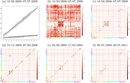
We illustrate the inadequacy of the sparsity assumption on a volatility panel dataset (see Section 5.3 for its description). Figure 1(a) shows that as the dimensionality increases, the leading eigenvalue of the spectral density matrix at frequency 0 (i.e., the long-run covariance) estimated from the data also increases linearly. This indicates the presence of strong serial and cross-sectional correlations that cannot be accommodated by sparse VAR models. In Figure 1(b), we report the logged and truncated p-values obtained from fitting a VAR(5) model to the same dataset (truncation level chosen at $\hspace{0.17em}\log \hspace{0.17em}(3.858\times {10}^{-6})$ by Bonferroni correction with the significance level 0.1) via ridge regression, see Cule, Vineis, and De Iorio (2011). Strong dependence observed from most pairs of the variables further confirms that we cannot infer a sparse pairwise relationship from such data. On the other hand, Figure 1(c) shows that once we estimate factors driving the strong correlations and adjust for their presence, there is evidence that the remaining dependence in the data can be modeled as being sparse. Together, the plots (d), (e), (c), and (f) display that the relationship between a pair of variables (after factor-adjustment) varies over time, particularly at the level of industrial sectors. Here, the intervals are chosen according to the data segmentation result reported in Section 5.3. This example highlights the importance of (i) accounting for the dominant correlations prior to fitting a model under the sparsity assumption, and (ii) detecting structural changes when analyzing time series datasets covering a long period.

Fig. 1 (a) The two largest eigenvalues of the long-run covariance matrix estimated from the volatility panel analyzed in Section 5.3 (March 18, 2008–July 07, 2009, n = 223) with subsets of cross-sections randomly sampled 100 times for each given dimension $p\in \{5,\dots ,72\}$ (x-axis). (b) and (c): logged and truncated p-values from fitting a VAR(5) model to the same dataset without and with factor-adjustment. (d)–(f): logged and truncated p-values similarly obtained with factor-adjustment from the same variables over different periods. In (b)–(f), for each pair of variables, the minimum p-value over the five lags is reported. Corresponding tickers are given in x- and y-axes and industrial sectors are indicated by the colors and boundaries drawn.

Motivated by the aforementioned characteristics of high-dimensional time series data, factor-adjusted regression modeling has increasingly gained popularity (Fan, Ke, and Wang 2020; Fan, Masini, and Medeiros 2021; Krampe and Margaritella 2021). The factor-adjusted VAR model proposed by Barigozzi, Cho, and Owens (2022) assumes that a handful of common factors capture strong serial and cross-sectional correlations, such that it is reasonable to assume a sparse VAR model on the remaining component to capture idiosyncratic, variable-specific dependence. We extend this framework by proposing a new, piecewise stationary factor-adjusted VAR model and develop FVARseg, an accompanying change point detection methodology. Below we summarize the methodological and theoretical contributions made in this article.

1.1 Generality of the Modeling Framework

We decompose the data into two piecewise stationary latent processes: one is driven by factors and accounts for dominant serial and cross-sectional correlations, and the other models sparse pairwise dependence via a VAR model. We adopt the most general approach to factor modeling and allow both components to undergo changes which, in the case of the latter, are attributed to shifts in the VAR parameters. To the best of our knowledge, such a general model simultaneously permitting the presence of common factors and change points, has not been studied in the literature previously. Accordingly, we are not aware of any method that can comprehensively address the data segmentation problem considered in this article.

1.2 Methodological Novelty

The idea of scanning the data for changes over moving windows, has successfully been applied to a variety of data segmentation problems (Preuss, Puchstein, and Dette 2015; Eichinger and Kirch 2018; Chen, Wang, and Wu 2022). We propose FVARseg, a two-stage methodology that combines this idea with statistics carefully designed to have good detection power against different types of changes in the two latent components. In Stage 1 of FVARseg, motivated by that dominant factor-driven correlations appear as leading eigenvalues in the frequency domain, see for example, Figure 1(a), we propose a detector statistic that contrasts the local spectral density matrix estimators from neighboring moving windows in operator norm, which is well-suited to detect changes in the factor-driven component.

In Stage 2 for detecting change points in the latent piecewise stationary VAR process, we deliberately avoid estimating the latent process which may incur large errors. Instead, we make use of (i) the Yule-Walker equation that relates autocovariances (ACV) and VAR parameters, and (ii) the availability of local ACV estimators of the latent VAR process after Stage 1. Combining these ingredients, we propose a novel detector statistic that enjoys methodological simplicity as well as statistical efficiency. Further, through sequential evaluation of the detector statistic, the second-stage procedure requires the estimation of local VAR parameters at selected locations only. Consequently it is highly competitive computationally when both the sample size and the dimensionality are large.

1.3 Theoretical Consistency

FVARseg achieves consistency in estimating the total number and locations of the change points in both of the piecewise stationary factor-driven and VAR processes. Our theoretical analysis is conducted in a setting considerably more general than those commonly adopted in the literature, permitting dependence across stationary segments and heavy-tailedness of the data. We also derive the rate of localization for each stage of FVARseg where we make explicit the influence of tail behavior and the size of changes. In particular, under Gaussianity, the estimators from Stage 1 nearly matches the minimax optimal rate derived for the simpler, covariance change point detection problem.

The rest of the article is structured as follows. Section 2 introduces the piecewise stationary factor-adjusted VAR model. Section 3 describes the two stages of FVARseg, the proposed data segmentation methodology, and Section 4 establishes its theoretical consistency. Section 5 demonstrates the performance of FVARseg empirically, and Section 6 concludes the article. R code is available from https://github.com/haeran-cho/fvarseg.

1.4 Notation

Let $\mathbf{I}$ and $\mathbf{O}$ denote an identity matrix and a matrix of zeros whose dimensions depend on the context. For a random variable X and $\nu \ge 1$, denote $\left|\right|X|{|}_{\nu }={(\mathsf{E}|X{|}^{\nu })}^{1/\nu }$. Given $\mathbf{A}=[a_{ii\prime }, 1\le i\le m, 1\le i\prime \le n]$, we denote by ${\mathbf{A}}^{*}$ its transposed complex conjugate. We define its element-wise ${\mathcal{l}}_{\infty },{\mathcal{l}}_1$ and ${\mathcal{l}}_2$-norms by $|\mathbf{A}{|}_{\infty }={\max }_{i,i\prime }|a_{ii\prime }|$, $|\mathbf{A}{|}_1=\sum _{i,i\prime }|a_{ii\prime }|$ and $|\mathbf{A}{|}_2=\sqrt{\sum _{i,i\prime }|a_{ii\prime }{|}^2}$, and its spectral and induced L₁, $L_{\infty }$-norms by $\left|\right|\mathbf{A}\left|\right|$, $\left|\right|\mathbf{A}|{|}_1={\max }_{1\le i\prime \le n}{\sum }_{i=1}^m|a_{ii\prime }|$ and $\left|\right|\mathbf{A}|{|}_{\infty }={\max }_{1\le i\le n}{\sum }_{i\prime =1}^m|a_{ii\prime }|$, respectively. For positive definite $\mathbf{A}$, we denote its minimum eigenvalue by $\left|\right|\mathbf{A}|{|}_{\min }$. For two real numbers, $a\vee b=\max (a,b)$ and $a\wedge b=\min (a,b)$. For two sequences $\left\{a_n\right\}$ and $\left\{b_n\right\}$, we write $a_n\asymp b_n$ if, for some constants $C_1,C_2>0$, there exists $N\in \mathbb{N}$ such that $C_1\le a_n{b}_n^{-1}\le C_2$ for all $n\ge N$.

2 Piecewise Stationary Factor-Adjusted VAR Model

2.1 Background

A zero-mean, p-variate process ${\mathit{\xi }}_t$ follows a VAR(d) model if it satisfies (1) $${\mathit{\xi }}_t={\mathit{A}}_1{\mathit{\xi }}_{t-1}+\cdots +{\mathit{A}}_d{\mathit{\xi }}_{t-d}+{(\mathbf{\Gamma })}^{1/2}{\mathit{\epsilon }}_t,$$(1) where ${\mathbf{A}}_{\mathcal{l}}\in {\mathbb{R}}^{p\times p}, 1\le \mathcal{l}\le d$, determine how future values of the series depend on their past. The p-variate random vector ${\mathit{\epsilon }}_t={({\epsilon }_{1t},\dots ,{\epsilon }_{pt})}^{\top }$ has ${\epsilon }_{it}$ which are iid for all i and t with $\mathsf{E}({\epsilon }_{it})=0$ and $\mathsf{var}({\epsilon }_{it})=1$. The positive definite matrix $\mathbf{\Gamma }\in {\mathbb{R}}^{p\times p}$ is the covariance matrix of the innovations for the VAR process.

A factor-driven component exhibits strong cross-sectional and/or serial correlations by “loading” finite-dimensional factors linearly. Among many, the generalized dynamic factor model (GDFM, Forni et al. 2000, 2015) provides the most general approach (see Appendix D for further discussions), and defines the p-variate factor-driven component ${\mathit{\chi }}_t$ as (2) $${\mathit{\chi }}_t=\mathcal{B}(L){\mathit{u}}_t=\sum _{\mathcal{l}=0}^{\infty }{\mathit{B}}_{\mathcal{l}}{\mathit{u}}_{t-\mathcal{l}}.$$(2)

For fixed q, the q-variate random vector ${\mathbf{u}}_t={(u_{1t},\dots ,u_{qt})}^{\top }$ contains the common factors which are shared across the variables and time, and u_jt are assumed to be iid for all j and t with $\mathrm{E}(u_{jt})=0$ and $\text{var}(u_{jt})=1$. The matrix of square-summable filters $\mathcal{B}(L)={\sum }_{\mathcal{l}=0}^{\infty }{\mathbf{B}}_{\mathcal{l}}{L}^{\mathcal{l}}$ with the lag-operator L and ${\mathbf{B}}_{\mathcal{l}}\in {\mathbb{R}}^{p\times q}$, serves the role of loadings under (2).

Barigozzi, Cho, and Owens (2022) propose a factor-adjusted VAR model, where the observations are assumed to be decomposed as a sum of the two latent components ${\mathit{\xi }}_t$ and ${\mathit{\chi }}_t$ in (1)–(2), with pervasive correlations in the data are accounted for by ${\mathit{\chi }}_t$ and the remaining dependence captured by ${\mathit{\xi }}_t$. In the next section, we introduce its piecewise stationary extension where both the factor-driven and VAR processes are allowed to undergo structural changes.

2.2 Model

We observe a zero-mean, p-variate piecewise stationary process ${\mathbf{X}}_t={\mathit{\chi }}_t+{\mathit{\xi }}_t$ where (3) $$\{\mathrm{}\mathrm{}\begin{array}{c}{\mathit{\chi }}_t={\mathit{\chi }}_t^{\left[k\right]}={\mathcal{B}}^{\left[k\right]}(L){\mathit{u}}_t\hfill \\ \mathrm{\hspace{1em}}\mathrm{\hspace{1em}}\hspace{1em}\text{for}{\theta }_{\chi ,k}+1\le t\le {\theta }_{\chi ,k+1}, 0\le k\le K_{\chi },\hfill \\ {\mathit{\xi }}_t={\mathit{\xi }}_t^{\left[k\right]}=\sum _{\mathcal{l}=1}^d{\mathit{A}}_{\mathcal{l}}^{\left[k\right]}{\mathit{\xi }}_{t-\mathcal{l}}+{({\mathbf{\Gamma }}^{\left[k\right]})}^{1/2}{\mathit{\epsilon }}_t\hfill \\ \mathrm{\hspace{1em}}\mathrm{\hspace{1em}}\hspace{1em}\text{for}{\theta }_{\xi ,k}+1\le t\le {\theta }_{\xi ,k+1}, 0\le k\le K_{\xi }.\hfill \end{array}$$(3)

Here, ${\theta }_{\chi ,k}, 1\le k\le K_{\chi }$, denote the change points in the piecewise stationary factor-driven component ${\mathit{\chi }}_t$ such that at each ${\theta }_{\chi ,k}$, the filter of loadings ${\mathcal{B}}^{[k]}(L)$ undergoes a change. We permit the factor number to vary over time as $q_k\le q$, with the factor ${\mathbf{u}}_t^{[k]}\in {\mathbb{R}}^{q_k}$ associated with ${\mathit{\chi }}_t^{[k]}$ being a sub-vector of ${\mathbf{u}}_t\in {\mathbb{R}}^q$. Similarly, ${\theta }_{\xi ,k}, 1\le k\le K_{\xi }$, denote the change points in the piecewise stationary VAR process ${\mathit{\xi }}_t$ at which the VAR parameters undergo shifts; we permit the VAR innovation covariance matrix to vary as ${\mathbf{\Gamma }}^{[k]}$ but our interest lies in detecting changes in VAR parameters, and the VAR order may vary over time as $d_k\le d$ with ${\mathbf{A}}_{\mathcal{l}}^{[k]}=\mathbf{O}$ for $\mathcal{l}\ge d_k+1$. By convention, we denote ${\theta }_{\chi ,0}={\theta }_{\xi ,0}=0$ and ${\theta }_{\chi ,K_{\chi }+1}={\theta }_{\xi ,K_{\xi }+1}=n$. In line with the factor modeling literature, we assume that ${\mathit{\chi }}_t$ and ${\mathit{\xi }}_t$ are uncorrelated through having $\mathrm{E}(u_{jt}{\epsilon }_{it\prime }) = 0$ for any i, j, t and $t\prime$.

The model (3) does not require that the change points in ${\mathit{\chi }}_t$ and ${\mathit{\xi }}_t$ are aligned, or that $K_{\chi }=K_{\xi }$. Our goal is to estimate the total number and locations of the change points for both of the piecewise stationary latent processes. Importantly, we allow $\{{\mathit{\xi }}_t^{[k]}, t\in \mathbb{Z}\}$ (resp. $\{{\mathit{\chi }}_t^{[k]}, t\in \mathbb{Z}\}$) to be dependent across k through sharing the innovations ${\mathit{\epsilon }}_t$ (resp. ${\mathbf{u}}_t$). This makes our model considerably more general than those found in the literature on (high-dimensional) data segmentation under VAR models (Wang et al. 2019; Safikhani and Shojaie 2022; Bai, Safikhani, and Michailidis 2022) which assume independence across the segments. Data segmentation under factor models has been considered by Barigozzi, Cho, and Fryzlewicz (2018) and Li, Li, and Fryzlewicz (2023) but they adopt a static approach to factor modeling.

2.3 Assumptions

We introduce assumptions that ensure the (asymptotic) identifiability of the two latent processes in (3) which are framed in terms of spectral properties, as well as controlling the degree of dependence in the data. Denote by ${\mathbf{\Gamma }}_{\chi }^{[k]}(\mathcal{l})=\mathrm{E}({\mathit{\chi }}_{t-\mathcal{l}}^{[k]}{({\mathit{\chi }}_t^{[k]})}^{\top })$ the ACV matrix of ${\mathit{\chi }}_t^{[k]}$ at lag $\mathcal{l}\in \mathbb{Z}$, and its spectral density matrix at frequency $\omega \in [-\pi ,\pi ]$ by ${\mathbf{\Sigma }}_{\chi }^{[k]}(\omega )={(2\pi )}^{-1}{\sum }_{\mathcal{l}=-\infty }^{\infty }{\mathbf{\Gamma }}_{\chi }^{[k]}(\mathcal{l})e^{-\iota \mathcal{l}\omega }$ with $\iota =\sqrt{-1}$. Then, ${\mu }_{\chi ,j}^{[k]}(\omega ), 1\le j\le q_k$, denote the real, positive eigenvalues of ${\mathbf{\Sigma }}_{\chi }^{[k]}(\omega )$ ordered by decreasing size. We similarly define ${\mathbf{\Gamma }}_{\xi }^{[k]}(\mathcal{l}),{\mathbf{\Sigma }}_{\xi }^{[k]}(\omega )$ and ${\mu }_{\xi ,j}^{[k]}(\omega )$ for ${\mathit{\xi }}_t^{[k]}$.

Assumption 2.1.

For each $0\le k\le K_{\chi }$, the following holds: There exist a positive integer $p_0\ge 1$, pairs of functions $\omega \mapsto {\alpha }_j^{[k]}(\omega )$ and $\omega \mapsto {\beta }_j^{[k]}(\omega )$ for $\omega \in [-\pi ,\pi ]$ and $1\le j\le q_k$, and $r_{k,j}\in (0,1]$ satisfying $r_{k,1}\ge \cdots \ge r_{k,q_k}$ such that for all $p\ge p_0$, $$\begin{array}{c}{\beta }_1^{\left[k\right]}(\omega )\ge \frac{{\mu }_{\chi ,1}^{\left[k\right]}(\omega )}{p^{r_{k,1}}}\ge {\alpha }_1^{\left[k\right]}(\omega )>\cdots >{\beta }_{q_k}^{\left[k\right]}(\omega )\\ \ge \frac{{\mu }_{q_k}^{\left[k\right]}(\omega )}{p^{r_{k,q_k}}}\ge {\alpha }_{q_k}^{\left[k\right]}(\omega )>0.\end{array}$$

If $r_{k,j}=1$ for all $1\le j\le q_k$ as frequently assumed in the literature (Fan, Liao, and Mincheva 2013; Forni et al. 2015), we are in the presence of q_k factors which are equally pervasive for the whole cross-sections of ${\mathit{\chi }}_t^{[k]}$. If $r_{k,j}<1$ for some j, we permit the presence of ‘weak’ factors. Since our primary interest lies in change point analysis, we later introduce a related but distinct condition on the size of change in ${\mathit{\chi }}_t$ in Assumption 4.2.

Assumption 2.2.

1. $\det ({\sum }_{\mathcal{l}=1}^d{\mathbf{A}}_{\mathcal{l}}^{[k]}{z}^{\mathcal{l}})\ne 0$ for all $\left|z\right|\le 1$ and $0\le k\le K_{\xi }$.

2. $m_{\epsilon }\le {\min }_{0\le k\le K_{\xi }}\left|\right|{\mathbf{\Gamma }}^{[k]}|{|}_{\min }\le {\max }_{0\le k\le K_{\xi }}|\left|{\mathbf{\Gamma }}^{[k]}\right||\le M_{\epsilon }$ for some constants $0<m_{\epsilon }\le M_{\epsilon }$.

3. Consider the Wold decomposition ${\mathit{\xi }}_t^{[k]}={\sum }_{\mathcal{l}=0}^{\infty }{\mathbf{D}}_{\mathcal{l}}^{[k]}{({\mathbf{\Gamma }}^{[k]})}^{1/2}{\mathit{\epsilon }}_{t-\mathcal{l}}$ where ${\mathbf{D}}_{\mathcal{l}}^{[k]}=[D_{\mathcal{l},ij}^{[k]}, 1\le i,j\le p]$. Then, there exist constants $\Xi >0$ and $\varsigma >2$ such that we have $C_{ij}, 1\le i,j\le p$, satisfying $\max \{{\max }_{1\le j\le p}{\sum }_{i=1}^p{C}_{ij},{\max }_{1\le i\le p}{\sum }_{j=1}^p{C}_{ij},{\max }_{1\le i\le p}\sqrt{{\sum }_{j=1}^p{C}_{ij}^2}\}\le \Xi$ with which ${\max }_{0\le k\le K_{\xi }}\left|D_{\mathcal{l},ij}^{[k]}\right|\le C_{ij}{(1+\mathcal{l})}^{-\varsigma }$ for all $\mathcal{l}\ge 0$.

4. ${\min }_{0\le k\le K_{\xi }}\underset{\omega \in [-\pi ,\pi ]}{\inf }{\mu }_{\xi ,p}^{[k]}(\omega )\ge m_{\xi }$ for some fixed constant $m_{\xi }>0$.

Assumption 2.3.

There exist constants $\Xi >0$ and $\varsigma >2$ such that for all $\mathcal{l}\ge 0$, $$\begin{array}{c}\underset{{}_{0\le k\le K_{\chi }}}{\max }\underset{{}_{1\le i\le p}}{\max }|{\mathit{B}}_{\mathcal{l},i·}^{\left[k\right]}{|}_2\le \Xi {(1+\mathcal{l})}^{-\varsigma }\text{and}\\ \underset{{}_{0\le k\le K_{\chi }}}{\max }\sqrt{\sum _{j=1}^{q_k}|{\mathit{B}}_{\mathcal{l},·j}^{\left[k\right]}{|}_{\infty }^2}\le \Xi {(1+\mathcal{l})}^{-\varsigma }.\end{array}$$

Assumption 2.2(i)–(ii) are standard conditions in the literature (Lütkepohl 2005; Basu and Michailidis 2015). Under condition (iii) and Assumption 2.3, we have time-varying serial dependence in ${\mathbf{X}}_t$ (across all segments) decay at an algebraic rate. Assumption 2.2(iii) allows for mild cross-correlations in ${\mathit{\xi }}_t^{[k]}$ while ensuring that ${\mu }_{\xi ,1}^{[k]}(\omega )$ is uniformly bounded:

Proposition 2.1.

Under Assumption 2.2, uniformly over all $\omega \in [-\pi ,\pi ]$, there exists some $M_{\xi }>0$ depending only on $M_{\epsilon }$, Ξ and Ϛ such that ${\max }_{0\le k\le K_{\xi }}\underset{\omega \in [-\pi ,\pi ]}{\sup }{\mu }_{\xi ,1}^{[k]}(\omega )\le M_{\xi }$.

Remark 2.1.

Proposition 2.1, together with Assumption 2.2(iv), establishes the boundedness of the eigenvalues of ${\mathbf{\Sigma }}_{\xi }^{[k]}(\omega )$, which is commonly assumed in the high-dimensional VAR literature for the consistency of Lasso estimators. Assumption 2.2(iv) holds if there exists some constant $\Xi <\infty$ satisfying $\max ({\max }_{1\le j\le p}{\sum }_{\mathcal{l}=1}^d|{\mathbf{A}}_{\mathcal{l},·j}^{[k]}{|}_1,{\max }_{1\le i\le p}{\sum }_{\mathcal{l}=1}^d|{\mathbf{A}}_{\mathcal{l},i·}^{[k]}{|}_1)\le \Xi$ (Basu and Michailidis 2015). When d = 1, we have ${\mathbf{D}}_{\mathcal{l}}^{[k]}={({\mathbf{A}}_1^{[k]})}^{\mathcal{l}}$ such that if $|{\mathbf{A}}_1^{[k]}{|}_{\infty }\le \gamma <1$, Assumption 2.2(iii) is readily satisfied with $\max (|\left|{\mathbf{D}}_{\mathcal{l}}^{[k]}\right|{|}_1,\left|\right|{\mathbf{D}}_{\mathcal{l}}^{[k]}|{|}_{\infty })\le \Xi {\gamma }^{\mathcal{l}-1}$.

From Assumption 2.1 and Proposition 2.1, the latent components in (3) are asymptotically identifiable as $p\to \infty$, thanks to the gap between ${\mu }_{\chi ,q_k}^{[k]}(\omega )$ diverging with p and ${\mu }_{\xi ,1}^{[k]}(\omega )$ which is uniformly bounded, which agrees with the phenomenon observed in Figure 1(a).

3 Methodology

3.1 Stage 1: Factor-Driven Component Segmentation

3.1.1 Change Point Detection

The spectral density matrix of ${\mathit{\chi }}_t$ is given by ${\mathbf{\Sigma }}_{\chi }^{[k]}(\omega )={(2\pi )}^{-1}{\mathcal{B}}^{[k]}(e^{-\iota \omega }){({\mathcal{B}}^{[k]}(e^{-\iota \omega }))}^{*}$ for ${\theta }_{\chi ,k}+1\le t\le {\chi }_{\chi ,k+1}$, that is it varies over time in a piecewise constant manner with change points at ${\theta }_{\chi ,k}, 1\le k\le K_{\chi }$. By Weyl’s inequality, Assumption 2.1 and Proposition 2.1 jointly indicate a gap in the eigenvalues of (time-varying) spectral density matrix of ${\mathbf{X}}_t$, that is, those attributed to the factor-driven component diverges with p while the remaining ones are bounded for all p. This suggests an approach that looks for changes in ${\mathit{\chi }}_t$ from the behavior of ${\mathbf{X}}_t$ in the frequency domain which we further justify below.

Example 3.1.

Suppose that ${\mathit{\chi }}_t$ contains a single change point at $t={\theta }_{\chi ,1}$ at which a new factor is introduced, that is ${\mathit{\chi }}_t^{[0]}={\mathcal{B}}^{[0]}(L){\mathbf{u}}_t^{[0]}$ and ${\mathit{\chi }}_t^{[1]}={\mathcal{B}}^{[1]}(L){\mathbf{u}}_t^{[1]}={\mathcal{B}}^{[0]}(L){\mathbf{u}}_t^{[0]}+\mathbf{b}(L)v_t$ with ${\mathbf{u}}_t^{[1]}={({({\mathbf{u}}_t^{[0]})}^{\top },v_t)}^{\top }$, which leads to ${\mathbf{\Sigma }}_{\chi }^{[1]}(\omega )-{\mathbf{\Sigma }}_{\chi }^{[0]}(\omega )=\mathbf{b}(e^{-\iota \omega }){\mathbf{b}}^{*}(e^{-\iota \omega })/(2\pi )$. Then, from the uncorrelatedness between ${\mathit{\chi }}_t$ and ${\mathit{\xi }}_t$ and Proposition 2.1, the time-varying spectral density of ${\mathbf{X}}_t,{\mathbf{\Sigma }}_{x,t}(\omega )$, satisfies $\left|\right|{\sum }_{t=1}^{{\theta }_{\chi ,1}}{\mathbf{\Sigma }}_{x,t}(\omega )/{\theta }_{\chi ,1}-{\sum }_{t={\theta }_{\chi ,1}+1}^n{\mathbf{\Sigma }}_{x,t}(\omega )/(n-{\theta }_{\chi ,1})\left|\right|=\left|\right|\mathbf{b}(e^{-\iota \omega }){\mathbf{b}}^{*}(e^{-\iota \omega })\left|\right|/(2\pi )+O(1)$. That is, the change in the spectral density of ${\mathit{\chi }}_t$ is detectable as a change in time-varying spectral density matrix of ${\mathbf{X}}_t$ in operator norm, with the size of change diverging with p as $\left|\right|{(\mathbf{b}(e^{-\iota \omega }))}^{*}\mathbf{b}(e^{-\iota \omega })\left|\right|$ does so under Assumption 2.1.

Thus, we detect changes in ${\mathit{\chi }}_t$ by scanning for any large change in the spectral density matrix of ${\mathbf{X}}_t$ measured in operator norm, and propose the following moving window-based approach. Given a bandwidth G, we estimate the local spectral density matrix of ${\mathbf{X}}_t$ by (4) $$\begin{array}{c}{\widehat{\mathbf{\Sigma }}}_{x,v}(\omega ,G)=\frac{1}{2\pi }\sum _{\mathcal{l}=-m}^{m}K\left(\frac{\mathcal{l}}{m}\right){\widehat{\mathbf{\Gamma }}}_{x,v}(\mathcal{l},G)\hspace{0.17em}\exp \hspace{0.17em}(-\iota \mathcal{l}\omega )\\ \text{for}\hspace{1em}G\le v\le n,\end{array}$$(4) where $K(·)$ denotes the Bartlett kernel, $m=G^{\beta }$ the kernel bandwidth with $\beta \in (0,1)$, and (5) $$\begin{array}{c}{\widehat{\mathbf{\Gamma }}}_{x,v}(\mathcal{l},G)=\frac{1}{G}\sum _{t=v-G+1+\mathcal{l}}^v{\mathit{X}}_{t-\mathcal{l}}{\mathit{X}}_t^{\top }\text{ for }\mathcal{l}\ge 0,\text{and}\\ {\widehat{\mathbf{\Gamma }}}_{x,v}(\mathcal{l},G)={\widehat{\mathbf{\Gamma }}}_{x,v}^{\top }(-\mathcal{l},G)\text{ for }\mathcal{l}<0.\end{array}$$(5)

Then the following statistic (6) $$T_{\chi ,v}(\omega ,G)=\left||{\widehat{\mathbf{\Sigma }}}_{x,v}(\omega ,G)-{\widehat{\mathbf{\Sigma }}}_{x,v+G}(\omega ,G)\right||,\hspace{1em}G\le v\le n-G,$$(6) serves as a good proxy of the difference in local spectral density matrices of ${\mathit{\chi }}_t$ over $I_v(G)=\{v-G+1,\dots ,v\}$ and $I_{v+G}(G)=\{v+1,\dots ,v+G\}$. To make it more precise, let ${\mathbf{\Sigma }}_{\chi ,v}(\omega ,G)$ denote a weighted average ${\sum }_{k=0}^{K_{\chi }}{w}_{\chi ,k}(v){\mathbf{\Sigma }}_{\chi }^{[k]}(\omega )$ with weights $w_{\chi ,k}(v)$ corresponding to the proportion of ${\mathit{\chi }}_t, t\in I_v(G)$, belonging to ${\mathit{\chi }}_t^{[k]}$ (see F.1). Then, $T_{\chi ,v}^{*}(\omega ,G)=\left|\right|{\mathbf{\Sigma }}_{\chi ,v}(\omega ,G)-{\mathbf{\Sigma }}_{\chi ,v+G}(\omega ,G)\left|\right|$, as a function of v, linearly increases and then decreases around the change points with a peak of size $\left|\right|{\mathbf{\Sigma }}_{\chi }^{[k]}(\omega )-{\mathbf{\Sigma }}_{\chi }^{[k+1]}(\omega )\left|\right|$ formed at $v={\theta }_{\chi ,k}$ for all $1\le k\le K_{\chi }$, provided that the bandwidth G is not too large (in the sense of Assumption 4.2(ii)). The detector statistic $T_{\chi ,v}(\omega ,G)$ is designed to approximate $T_{\chi ,v}^{*}(\omega ,G)$ when ${\mathit{\chi }}_t$ is not directly observed, and thus is well-suited to detect and locate the change points therein. Unlike other methods for detecting changes in the factor structure (e.g., Li, Li, and Fryzlewicz 2023), we do not require the number of factors, either for each segment or for the whole dataset, as an input for the construction of $T_{\chi ,v}(\omega ,G)$.

Once $T_{\chi ,v}({\omega }_l,G)$ is evaluated at the Fourier frequencies ${\omega }_l=2\pi l/(2m+1), 0\le l\le m$, we adapt the maximum-check of Eichinger and Kirch (2018) for simultaneous detection of the multiple change points. Taking the pointwise maximum over the frequencies at each given location v, we check if $T_{\chi ,v}(\omega (v),G)$ exceeds some threshold ${\kappa }_{n,p}$ where $\omega (v)$ denotes the frequency at which $T_v({\omega }_l,G)$ is maximized, that is $\omega (v)=\arg {\max }_{{\omega }_l:\mathrm{ }0\le l\le m}{T}_v({\omega }_l,G)$. If so, it provides evidence that a change point ${\theta }_{\chi ,k}$ is located near the time point v, but some care is needed to avoid detecting duplicate estimators, since the detector statistic is expected to take a large value over an interval containing ${\theta }_{\chi ,k}$. Therefore, denoting by $\mathcal{I}\subset \{G,\dots ,n-G\}$ the set containing all time points at which $T_{\chi ,v}(\omega (v),G)>{\kappa }_{n,p}$, we regard $\widehat{\theta }=\arg {\max }_{v\in \mathcal{I}}{T}_{\chi ,v}(\omega (v),G)$ as a change point estimator if it is a local maximizer of $T_{\chi ,v}(\omega (\widehat{\theta }),G)$ within an interval of radius ηG centered at $\widehat{\theta }$ with some $\eta \in (0,1)$, that is $T_{\chi ,\widehat{\theta }}(\omega (\widehat{\theta }),G)\ge {\max }_{\widehat{\theta }-\eta G<v\le \widehat{\theta }+\eta G}{T}_{\chi ,v}(\omega (\widehat{\theta }),G)$. Once $\widehat{\theta }$ is added to the set of final estimators, say ${\widehat{\Theta }}_{\chi }$, in order to avoid the risk of duplicate estimators, we remove the interval of radius G centered at $\widehat{\theta }$ from $\mathcal{I}$, and repeat the same procedure with the maximizer of $T_{\chi ,v}(\omega (v),G)$ at time points v remaining in $\mathcal{I}$ until the set $\mathcal{I}$ is empty. Algorithm 1 in Appendix C outlines the steps of Stage 1 of FVARseg.

3.1.2 Post-Segmentation Factor Adjustment

Following the detection of change points in ${\mathit{\chi }}_t$, we are able to estimate the segment-specific quantities related to ${\mathit{\chi }}_t^{[k]}$. In view of the second-stage of FVARseg detecting change points in ${\mathit{\xi }}_t$, we describe how to estimate ${\mathbf{\Gamma }}_{\chi }^{[k]}(\mathcal{l})$ with which we can estimate the ACV of ${\mathit{\xi }}_t$.

For each $k=0,\dots ,{\widehat{K}}_{\chi }$, we first estimate the spectral density of ${\mathbf{X}}_t$ over the segment $\{{\widehat{\theta }}_{\chi ,k}+1,\dots ,{\widehat{\theta }}_{\chi ,k+1}\}$ by ${\widehat{\mathbf{\Sigma }}}_x^{[k]}(\omega )$ as in (4) using the sample ACV computed from the segment (we use the same kernel bandwidth m for simplicity). Then noting that the spectral density matrix of ${\mathit{\chi }}_t^{[k]}$ is of rank q_k under (3), we estimate it from the eigendecomposition of ${\widehat{\mathbf{\Sigma }}}_x^{[k]}({\omega }_l)$ by retaining only the q_k largest eigenvalues, say ${\widehat{\mu }}_{x,j}^{[k]}({\omega }_l)$, and the associated eigenvectors ${\widehat{\mathbf{e}}}_{x,j}^{[k]}({\omega }_l)$, and then estimate the ACV of ${\mathit{\chi }}_t^{[k]}$ by inverse Fourier transform, that is (7) $$\begin{array}{c}{\widehat{\mathbf{\Sigma }}}_{\chi }^{\left[k\right]}({\omega }_l)=\sum _{j=1}^{q_k}{\widehat{\mu }}_{x,j}^{\left[k\right]}({\omega }_l){\widehat{\mathit{e}}}_{x,j}^{\left[k\right]}({\omega }_l){\left({\widehat{\mathit{e}}}_{x,j}^{\left[k\right]}({\omega }_l)\right)}^{*}\text{ and }\\ {\widehat{\mathbf{\Gamma }}}_{\chi }^{\left[k\right]}(\mathcal{l})=\frac{2\pi }{2m+1}\sum _{l=-m}^m{\widehat{\mathbf{\Sigma }}}_{\chi }^{\left[k\right]}({\omega }_l)e^{\iota {\omega }_l\mathcal{l}}.\end{array}$$(7)

The estimators in (7) require the factor number q_k as an input. We refer to Hallin and Liška (2007) for an information criterion (IC)-based estimator of q_k that make use of the postulated eigengap in the spectral density matrix of ${\mathbf{X}}_t$.

3.2 Stage 2: Piecewise VAR Process Segmentation

Applying the existing VAR segmentation methods in our setting requires estimating the np elements of the latent piecewise stationary VAR process ${\mathit{\xi }}_t$, which introduces additional errors and possibly results in the loss of statistical efficiency. In addition, as discussed in Appendix A.2, the existing methods tend to be computationally demanding, for example by evaluating the Lasso estimators $O(n^2)$ times in a dynamic programming algorithm, or solving a large fused Lasso objective function of dimension $n{p}^{2}d$. Instead, since we can estimate the local ACV of ${\mathit{\xi }}_t$ from the post-segmentation factor-adjustment in Stage 1, our proposed methodology for segmenting the latent VAR component avoids estimating ${\mathit{\xi }}_t$ directly. Also, as described below, the proposed method evaluates the local VAR parameters at carefully selected locations only, and thus is computationally efficient.

Specifically, our approach makes use of the Yule-Walker equation (Lütkepohl 2005). Let ${\mathit{\beta }}^{[k]}={[{\mathbf{A}}_1^{[k]},\dots ,{\mathbf{A}}_d^{[k]}]}^{\top }\in {\mathbb{R}}^{(pd)\times p}$ contain all VAR parameters in the kth segment. Then, it is related to the ACV matrices ${\mathbf{\Gamma }}_{\xi }^{[k]}(\mathcal{l})=\mathsf{E}({\mathit{\xi }}_{t-\mathcal{l}}^{[k]}{({\mathit{\xi }}_t^{[k]})}^{\top })$ as ${\mathbb{G}}^{[k]}{\mathit{\beta }}^{[k]}={\mathbb{g}}^{[k]}$, where (8) $$\begin{array}{c}{\mathbb{G}}^{\left[k\right]}=\left[\begin{array}{cccc}{\mathbf{\Gamma }}_{\xi }^{\left[k\right]}(0)& {\mathbf{\Gamma }}_{\xi }^{\left[k\right]}(-1)& \dots & {\mathbf{\Gamma }}_{\xi }^{\left[k\right]}(-d+1)\\ & & \ddots & \\ {\mathbf{\Gamma }}_{\xi }^{\left[k\right]}(d-1)& {\mathbf{\Gamma }}_{\xi }^{\left[k\right]}(d-2)& \dots & {\mathbf{\Gamma }}_{\xi }^{\left[k\right]}(0)\end{array}\right]\\ \hspace{1em}\text{and}\hspace{1em}{\mathbb{g}}^{\left[k\right]}=\left[\begin{array}{c}{\mathbf{\Gamma }}_{\xi }^{\left[k\right]}(1)\\ ⋮\\ {\mathbf{\Gamma }}_{\xi }^{\left[k\right]}(d)\end{array}\right],\end{array}$$(8) with ${\mathbb{G}}^{[k]}$ being invertible due to Assumption 2.2(iv). We propose to use this estimating equation in combination with the local ACV estimators of ${\mathit{\xi }}_t$ obtained as described below.

For a given bandwidth G and the interval $I_v(G)=\{v-G+1,\dots ,v\}$, we estimate the ACV of ${\mathit{\xi }}_t$ for $t\in I_v(G)$, by ${\widehat{\mathbf{\Gamma }}}_{\xi ,v}(\mathcal{l},G)={\widehat{\mathbf{\Gamma }}}_{x,v}(\mathcal{l},G)-{\widehat{\mathbf{\Gamma }}}_{\chi ,v}(\mathcal{l},G)$. Here, ${\widehat{\mathbf{\Gamma }}}_{x,v}(\mathcal{l},G)$ is defined in (5) and ${\widehat{\mathbf{\Gamma }}}_{\chi ,v}(\mathcal{l},G)$ is a weighted average of ${\widehat{\mathbf{\Gamma }}}_{\chi }^{[k]}(\mathcal{l}), 0\le k\le {\widehat{K}}_{\chi }$, the estimators of ACV of ${\mathit{\chi }}_t^{[k]}$ in (7), with the weights given by the proportion of $I_v(G)$ covered by the kth segment (see F.16 for the precise definition). Replacing ${\mathbf{\Gamma }}_{\xi }^{[k]}(\mathcal{l})$ with ${\widehat{\mathbf{\Gamma }}}_{\xi ,v}(\mathcal{l},G)$, we obtain ${\widehat{\mathbb{G}}}_v(G)$ estimating a weighted average of ${\mathbb{G}}^{[k]}$, and similarly ${\widehat{\mathbb{g}}}_v(G)$. Then, we propose to scan $T_{\xi ,v}(\widehat{\mathit{\beta }},G)=\left|\right||({\widehat{\mathbb{G}}}_v(G)\widehat{\mathit{\beta }}-{\widehat{\mathbb{g}}}_v(G))-({\widehat{\mathbb{G}}}_{v+G}(G)\widehat{\mathit{\beta }}-{\widehat{\mathbb{g}}}_{v+G}(G))|\left|\right|$ with some inspection parameter $\widehat{\mathit{\beta }}\in {\mathbb{R}}^{(pd)\times p}$ and a matrix norm $\left|\right||·|\left|\right|$. We motivate this statistic by considering $T_{\xi ,v}^{*}(\widehat{\mathit{\beta }},G)=\left|\right||({\mathbb{G}}_v(G)\widehat{\mathit{\beta }}-{\mathbb{g}}_v(G))-({\mathbb{G}}_{v+G}(G)\widehat{\mathit{\beta }}-{\mathbb{g}}_{v+G}(G))|\left|\right|$, its population counterpart. With appropriately chosen G (see Assumption 4.4(ii)), $T_{\xi ,v}^{*}(\widehat{\mathit{\beta }},G)=0$ if v is far from all the change points in ${\mathit{\xi }}_t$, that is ${\min }_k|v-{\theta }_{\xi ,k}|\ge G$, while it is tent-shaped near the change points with a local maximum at $v={\theta }_{\xi ,k}$, provided that (9) $${\mathbb{G}}^{[k-1]}(\widehat{\mathit{\beta }}-{\mathit{\beta }}^{[k-1]})\ne {\mathbb{G}}^{\left[k\right]}(\widehat{\mathit{\beta }}-{\mathit{\beta }}^{\left[k\right]}).$$(9)

For the inspection parameter, we adopt an ${\mathcal{l}}_1$-regularized Yule-Walker estimator which, at some $v_{°}\in \{G,\dots ,n\}$, solves the following constrained ${\mathcal{l}}_1$-minimization problem (10) $$\begin{array}{c}{\widehat{\mathit{\beta }}}_{v_{°}}(G)=\arg {\min }_{\mathit{\beta }\in {\mathbb{R}}^{pd\times p}}|\mathit{\beta }{|}_1\hspace{1em}\text{subject to}\\ {\left|{\widehat{\mathbb{G}}}_{v_{°}}(G)\mathit{\beta }-{\widehat{\mathbb{g}}}_{v_{°}}(G)\right|}_{\infty }\le {\lambda }_{n,p},\end{array}$$(10) with a tuning parameter ${\lambda }_{n,p}>0$. Assuming stationarity, a similar approach has been proposed for the estimation of high-dimensional VAR in Han, Lu, and Liu (2015), and extended to the case where the VAR process of interest is latent in Barigozzi, Cho, and Owens (2022). The ${\mathcal{l}}_{\infty }$-constraint in (10) naturally leads to the choice $\left|\right||·|\left|\right|=|·{|}_{\infty }$, resulting in the following detector statistic: $$T_{\xi ,v}(\widehat{\mathit{\beta }},G)={\left|\left({\widehat{\mathbb{G}}}_v(G)\widehat{\mathit{\beta }}-{\widehat{\mathbb{g}}}_v(G)\right)-\left({\widehat{\mathbb{G}}}_{v+G}(G)\widehat{\mathit{\beta }}-{\widehat{\mathbb{g}}}_{v+G}(G)\right)\right|}_{\infty }.$$

For good detection power, the condition in (9) suggests using an estimator of ${\mathit{\beta }}^{[k-1]}$ or ${\mathit{\beta }}^{[k]}$ in place of $\widehat{\mathit{\beta }}$ for detecting ${\theta }_{\xi ,k}$. Therefore, we propose to evaluate $T_{\xi ,v}({\widehat{\mathit{\beta }}}_{v_{°}}(G),G)$ for $v\ge G$, with ${\widehat{\mathit{\beta }}}_{v_{°}}(G)$ updated sequentially at locations strategically selected as below.

First we estimate ${\mathit{\beta }}^{[0]}$ by $\widehat{\mathit{\beta }}={\widehat{\mathit{\beta }}}_G(G)$ in (10) with $v_{°}=G$ and scan the data using $T_{\xi ,v}(\widehat{\mathit{\beta }},G), v\ge v_{°}$. When $T_{\xi ,v}(\widehat{\mathit{\beta }},G)$ exceeds some threshold, say ${\pi }_{n,p}$, at $v=\check{\theta }$ for the first time, it signifies that a change has occurred in the neighborhood. Reducing the search for a change point to $\{\check{\theta },\dots ,\check{\theta }+G\}$, we identify a change point estimator as the local maximizer ${\widehat{\theta }}_{\xi ,1}=\arg {\max }_{\check{\theta }\le v\le \check{\theta }+G}{T}_{\xi ,v}(\widehat{\mathit{\beta }},G)$. Then updating $\widehat{\mathit{\beta }}$ with ${\widehat{\mathit{\beta }}}_{v_{°}}(G)$ obtained at $v_{°}={\widehat{\theta }}_{\xi ,1}+(\eta +1)G$ for some $\eta \in (0,1]$ (i.e., only using an interval of length G located strictly to the right of ${\widehat{\theta }}_{\xi ,1}$ for its computation), we continue screening $T_{\xi ,v}(\widehat{\mathit{\beta }},G), v\ge v_{°}$, until it next exceeds ${\pi }_{n,p}$. These steps of screening $T_{\xi ,v}(\widehat{\mathit{\beta }},G)$ and updating $\widehat{\mathit{\beta }}$ are repeated iteratively until the end of the data sequence is reached. Algorithm 2 in Appendix C outlines the steps of the Stage 2 methodology.

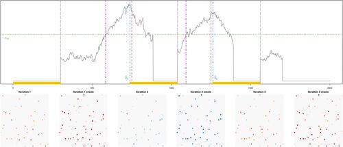
Figure 2 illustrates that although ${\mathit{\xi }}_t$ is latent, at each iteration, ${\widehat{\mathit{\beta }}}_{v_{°}}(G)$ does as well as its oracle counterpart (obtained as in (10) with the sample ACV of ${\mathit{\xi }}_t$ replacing ${\widehat{\mathbf{\Gamma }}}_{\xi ,v}(\mathcal{l},G)$). Computationally, this strategy benefits from that the costly solution to the ${\mathcal{l}}_1$-minimization problem in (10) is required (at most) $K_{\xi }+1$ times with an appropriately chosen threshold ${\pi }_{n,p}$ (see Theorem 4.3). We further demonstrate numerically the competitiveness of Stage 2 as a standalone method for VAR time series segmentation in Section 5.2, and provide an in-depth comparative study with the existing methods in Appendix A.2.

Fig. 2 Illustration of Stage 2 applied to a realization from (M1) of Section 5.2 with G = 300 and d = 1. Top: The solid curve represents $T_{\xi ,v}(\widehat{\mathit{\beta }},G), v_{°}\le v\le \check{\theta }+G$, computed at the three iterations of Steps 1–3 of Algorithm 2. At each iteration, we use $\widehat{\mathit{\beta }}={\widehat{\mathit{\beta }}}_{v_{°}}(G)$ estimated from each of the sections the data highlighted in the x-axis (left to right); the corresponding estimators are plotted in the bottom panel and for comparison, we also plot the estimators obtained in the oracle setting where ${\mathit{\xi }}_t$ is observable (all plots have the identical z-axis range). The locations of $v_{°},\check{\theta }$ and $\widehat{\theta }$ in Algorithm 2, and ${\theta }_{\xi ,k}$ are denoted by the vertical long-dashed, dot-dashed, dotted and dashed lines, respectively. The horizontal line represents ${\pi }_{n,p}$ chosen as described in Section 5.1.

4 Theoretical Properties

4.1 Consistency of Stage 1 of FVARseg

We carry out our theoretical investigation under two different regimes with respect to the tail behavior of ${\mathbf{u}}_t$ and ${\mathit{\xi }}_t$; in particular, the weaker condition in Assumption 4.1(i) permits heavy-tailed innovations, while the existing literature on (piecewise stationary) VAR modeling in high dimensions, commonly adopts the Gaussianity as in (ii).

Assumption 4.1.

We assume either of the following conditions.

1. There exists $\nu >4$ such that $\max \left\{\mathrm{E}(|u_{jt}{|}^{\nu }),\mathrm{E}(|{\epsilon }_{it}{|}^{\nu })\right\}\le {\mu }_{\nu }<\infty$.

2. ${\mathbf{u}}_t{\sim }_{\text{iid}}{\mathcal{N}}_q(\mathbf{0},\mathbf{I})$ and ${\mathit{\epsilon }}_t{\sim }_{\text{iid}}{\mathcal{N}}_p(\mathbf{0},\mathbf{I})$.

In establishing the consistency of Stage 1, we opt to measure the size of changes in ${\mathit{\chi }}_t$ using ${\mathbf{\Delta }}_{\chi ,k}(\omega )={\mathbf{\Sigma }}_{\chi }^{[k]}(\omega )-{\mathbf{\Sigma }}_{\chi }^{[k-1]}(\omega ),1\le k\le K_{\chi }$, the difference in spectral density matrices of ${\mathit{\chi }}_t$ from neighboring segments. As ${\mathbf{\Delta }}_{\chi ,k}(\omega )$ is Hermitian, we can always find the jth largest (in modulus), real-valued eigenvalue of ${\mathbf{\Delta }}_{\chi ,k}(\omega )$ which we denote by ${\mu }_j({\mathbf{\Delta }}_{\chi ,k}(\omega ))$, with ${\mu }_1({\mathbf{\Delta }}_{\chi ,k}(\omega ))=\left|\right|{\mathbf{\Delta }}_{\chi ,k}(\omega )\left|\right|$. Recall that $m=G^{\beta }$ for some $\beta \in (0,1)$, denotes the bandwidth used in local spectral density estimation, see (4).

Assumption 4.2.

1. For each $1\le k\le K_{\chi }$, the following holds: There exist a positive integer $p_0\ge 1$ and pairs of functions $\omega \mapsto a_j^{[k]}(\omega )$ and $\omega \mapsto b_j^{[k]}(\omega )$ for $\omega \in [-\pi ,\pi ]$ and j = 1, 2, and $r_{k,1}^{\prime }\in (0,1]$ and $r_{k,2}^{\prime }\in [0,1]$ satisfying $r_{k,1}^{\prime }\ge r_{k,2}^{\prime }$, such that $$\begin{array}{c}{b}_1^{\left[k\right]}(\omega )\ge \frac{{\mu }_1({\mathbf{\Delta }}_{\chi ,k}(\omega ))}{p^{r_{k,1}^{\prime }}}\ge a_1^{\left[k\right]}(\omega )>b_2^{\left[k\right]}(\omega )\\ \ge \frac{{\mu }_2({\mathbf{\Delta }}_{\chi ,k}(\omega ))}{p^{r_{k,2}^{\prime }}}\ge a_2^{\left[k\right]}(\omega )\ge 0\end{array}$$for all $p\ge p_0$. Besides, we assume that the functions $\omega \mapsto p^{-r_{k,1}^{\prime }}{\mu }_1({\mathbf{\Delta }}_{\chi ,k}(\omega ))$ are Lipschitz continuous with bounded Lipschitz constants. Then for ${\Delta }_{\chi ,k}={\max }_{\omega \in [-\pi ,\pi ]}{\mu }_1({\mathbf{\Delta }}_{\chi ,k}(\omega ))$, we have ${\max }_{1\le k\le K_{\chi }}{\Delta }_{\chi ,k}^{-1}·p({\psi }_n\vee m^{-1})=o(1)$, where (11) $${\psi }_n=\{\text{}\begin{array}{cc}\frac{n^{2/\nu }m{\hspace{0.17em}\log \hspace{0.17em}}^{2+2/\nu }(G)}{G}\vee \sqrt{\frac{m\hspace{0.17em}\log \hspace{0.17em}(n)}{G}}\hfill & \text{under Assumption} 4.1(\mathrm{i}),\hfill \\ \sqrt{\frac{m\hspace{0.17em}\log \hspace{0.17em}(n)}{G}}\hfill & \text{under Assumption} 4.1(\text{ii}).\hfill \end{array}$$(11)

2. The bandwidth G = G_n satisfies $G_n\to \infty$ as $n\to \infty$ while fulfilling (12) $$\min \left\{\underset{{}_{0\le k\le K_{\chi }}}{\min }({\theta }_{\chi ,k+1}-{\theta }_{\chi ,k}),\underset{{}_{0\le k\le K_{\xi }}}{\min }({\theta }_{\xi ,k+1}-{\theta }_{\xi ,k})\right\}\ge 2G.$$(12) Assumption 4.2 specifies the detection lower bound which is determined by ${\min }_k{\Delta }_{\chi ,k}$ and ${\min }_k({\theta }_{\chi ,k+1}-{\theta }_{\chi ,k})$ (through G), for all $K_{\chi }$ change points ${\mathit{\chi }}_t$ to be detectable by Stage 1. In the literature on change point detection in factor models, a common assumption is that the change is large enough to appear as extra “factors” (Duan, Bai, and Han 2022), in light of which the condition (i) is a reasonable one. It further requires ${\mu }_1({\mathbf{\Delta }}_{\chi ,k}(\omega ))$ to be distinct from the rest. In fact, the remaining ${\mu }_j({\mathbf{\Delta }}_{\chi ,k}(\omega )), j\ge 2$, are allowed to be exactly zero, which is the case in Example 3.1; here, we have ${\Delta }_{\chi ,1}={\max }_{\omega }{(2\pi )}^{-1}\left|\right|{(\mathbf{b}(e^{-\iota \omega }))}^{*}\mathbf{b}(e^{-\iota \omega })\left|\right|$ where $\mathbf{b}(z)$ is a p-variate vector of factor loading filters. The rate $p({\psi }_n\vee m^{-1})$ represents the bias-variance tradeoff when estimating the local spectral density matrix of ${\mathit{\chi }}_t$ by ${\widehat{\mathbf{\Sigma }}}_{x,v}(G,\omega )$ (see Proposition F.6). It is possible to find the rate of kernel bandwidth m that minimizes this rate depending on the tail behavior of X_it (e.g., $m\asymp {(G/\hspace{0.17em}\log \hspace{0.17em}(n))}^{1/3}$ under Gaussianity), but we choose to explicitly highlight the role of this tuning parameter on our results.

Theorem 4.1.

Suppose that Assumptions 2.1–2.3, 4.1, and 4.2 hold. Let ${\kappa }_{n,p}$ satisfy $$\begin{array}{c}2Mp\left({\psi }_n\vee \frac{1}{m}\vee \frac{1}{p}\right)<{\kappa }_{n,p}<\frac{1}{2}\underset{{}_{1\le k\le K_{\chi }}}{\min }{\Delta }_{\chi ,k}\\ \mathrm{\hspace{1em}}\mathrm{\hspace{1em}}-Mp\left({\psi }_n\vee \frac{1}{m}\vee \frac{1}{p}\right)\end{array}$$for some constant M > 0. Then, there exists a set ${\mathcal{M}}_{n,p}^{\chi }$ with $\mathsf{P}({\mathcal{M}}_{n,p}^{\chi })\to 1$ as $n,p\to \infty$, such that the following holds for ${\widehat{\Theta }}_{\chi }=\{{\widehat{\theta }}_{\chi ,k}, 1\le k\le {\widehat{K}}_{\chi }: {\widehat{\theta }}_{\chi ,1}<\cdots <{\widehat{\theta }}_{\chi ,{\widehat{K}}_{\chi }}\}$ returned by Stage 1 of FVARseg, on ${\mathcal{M}}_{n,p}^{\chi }$ for large enough n and p:

1. ${\widehat{K}}_{\chi }=K_{\chi }$ and ${\max }_{1\le k\le K_{\chi }}|{\widehat{\theta }}_{\chi ,k}-{\theta }_{\chi ,k}|\le {ϵ}_{0}G$ for some ${ϵ}_0\in (0,1/2)$ with $\eta \in (2{ϵ}_0,1]$.

2. There exists a constant $c_0>0$ such that for all $1\le k\le K_{\chi },|{\widehat{\theta }}_{\chi ,k}-{\theta }_{\chi ,k}|\le c_0{\rho }_{n,p}^{[k]}$ where $$\begin{array}{c}{\rho }_{n,p}^{\left[k\right]}={\left(\frac{{\Delta }_{\chi ,k}}{p}\right)}^{-2}\\ \hspace{1em}\times \{\begin{array}{cc}{m}^{\frac{\nu }{\nu -2}}{(G{K}_{\chi })}^{\frac{2}{\nu -2}}\hfill & \text{under Assumption} 4.1(\mathrm{i}),\hfill \\ m\hspace{0.17em}\log \hspace{0.17em}(G{K}_{\chi })\hfill & \text{under Assumption} 4.1(\text{ii}).\hfill \end{array}\end{array}$$

Remark 4.1.

1. In Theorem 4.1(b), ${\rho }_{n,p}^{[k]}$ reflects the difficulty associated with estimating the individual change point ${\theta }_{\chi ,k}$ manifested by ${(p^{-1}{\Delta }_{\chi ,k})}^{-2}$. In the Gaussian case (Assumption 4.1(ii)), the localization rate ${\rho }_{n,p}^{[k]}$ is always sharper than G due to Assumption 4.2(i). Considering the problem of covariance change point detection in independent, sub-Gaussian random vectors in high dimensions, Wang, Yu, and Rinaldo (2021) derive the minimax lower bound on the localization rate in their Lemma 3.2, and ${\rho }_{n,p}^{[k]}$ matches this rate up to $m\hspace{0.17em}\log \hspace{0.17em}(n)$; here, the dependence on the kernel bandwidth m is attributed to that we consider a time series segmentation problem, that is a change may occur in the ACV of ${\mathit{\chi }}_t$ at lags other than zero. If heavier tails are permitted (Assumption 4.1(i)), ${\rho }_{n,p}^{[k]}$ can be tighter than ${ϵ}_{0}G$, for example when ${\Delta }_{\chi ,k}\asymp p,K_{\chi }$ is fixed and $m\asymp G^{\beta }$ for some $\beta \in (0,1-4/\nu )$.

2. Empirically, replacing $\widehat{\theta }$ with $\tilde{\theta }=\arg {\max }_{v\in \mathcal{I}} {\text{avg}}_l{T}_{\chi ,v}({\omega }_l,G)$ returns a more stable location estimator, where ${\text{avg}}_l$ denotes the average operator over $l=0,\dots ,m$. We can derive the localization rate for $\tilde{\theta }$ similarly as in Theorem 4.1(b) with ${\tilde{\Delta }}_{\chi ,k}={\pi }^{-1}{\int }_0^{\pi }||{\mathbf{\Delta }}_{\chi ,k}(\omega )||d\omega$ in place of ${\Delta }_{\chi ,k}$. Our numerical results in Section 5.2 are based on this estimator.

Next, we establish the consistency of ${\widehat{\mathbf{\Gamma }}}_{\chi }^{[k]}(\mathcal{l})$ in (7) estimating the segment-specific ACV of ${\mathit{\chi }}_t^{[k]}$ under the following assumption on the strength of factors.

Assumption 4.3.

Assumption 2.1 holds with $r_{k,j}=1$ for all $1\le j\le q_k$ and $0\le k\le K_{\chi }$.

Theorem 4.2.

Suppose that Assumption 4.3 holds in addition to the assumptions made in Theorem 4.1, and define ${\rho }_{n,p}={\max }_{1\le k\le K_{\chi }}\min ({ϵ}_{0}G,{\rho }_{n,p}^{[k]})$. Also let $${\vartheta }_{n,p}=\{\text{}\begin{array}{cc}\frac{m{(np)}^{2/\nu }{\hspace{0.17em}\log \hspace{0.17em}}^{7/2}(p)}{G} \vee \sqrt{\frac{m\hspace{0.17em}\log \hspace{0.17em}(np)}{G}}& \text{under Assumption} 4.1(\mathrm{i}),\\ \sqrt{\frac{m\hspace{0.17em}\log \hspace{0.17em}(np)}{G}}& \text{under Assumption} 4.1(\text{ii}).\end{array}$$

Then on ${\mathcal{M}}_{n,p}^{\chi }$ defined in Theorem 4.1, for some finite integer $d\in \mathbb{N}$, we have $$\begin{array}{c}\underset{{}_{0\le k\le K_{\chi }}}{\max }\underset{{}_{0\le \mathcal{l}\le d}}{\max }{\left|{\widehat{\mathbf{\Gamma }}}_{\chi }^{\left[k\right]}(\mathcal{l})-{\mathbf{\Gamma }}_{\chi }^{\left[k\right]}(\mathcal{l})\right|}_{\infty }\\ \mathrm{\hspace{1em}}\mathrm{\hspace{1em}}=O_p\left({\vartheta }_{n,p}\vee \frac{1}{m}\vee \frac{{\rho }_{n,p}}{G}\vee \frac{1}{\sqrt{p}}\right).\end{array}$$

It is possible to work under the weaker Assumption 2.1 and trace the effect of weak factors or bound estimation errors measured in different norms. Corollary E.16 of Barigozzi, Cho, and Owens (2022) derives such results in the stationary setting, where an additional multiplicative factor of $p^{2(1-{\min }_k{r}_{k,q_k})}$ appears in the O_P-bound in Theorem (4.2). We work under the stronger Assumption 4.3 as it simplifies the presentation of Theorem 4.2 which plays an important role in the investigation into Stage 2 of FVARseg. Also, for the factor number estimator of Hallin and Liška (2007) which achieves consistency under the general dynamic factor model we adopt in (3), it is required that $r_{k,q_k}=1$ for all $0\le k\le K_{\chi }$. Forni et al. (2004) argue that this assumption is a natural one requiring the influence of the common shocks to be, in some sense, “stationary along the cross-sections,” and also it is compatible with the cross-sectional ordering being completely arbitrary.

4.2 Consistency of Stage 2 of FVARseg

Suppose that the tuning parameter for the ${\mathcal{l}}_1$-regularized Yule-Walker estimation problem in (10), is set with some constant M > 0 and ${\vartheta }_{n,p}$ and ${\rho }_{n,p}$ defined in Theorem 4.2, as (13) $${\lambda }_{n,p}=M\left(\underset{{}_{0\le k\le K_{\xi }}}{\max }\left|\right|{\mathit{\beta }}^{\left[k\right]}|{|}_1+1\right)\left({\vartheta }_{n,p}\vee \frac{1}{m}\vee \frac{{\rho }_{n,p}}{G}\vee \frac{1}{\sqrt{p}}\right).$$(13)

This choice reflects the error in ${\widehat{\mathbf{\Gamma }}}_{\xi ,v}(\mathcal{l},G)$ estimating the local ACV of ${\mathit{\xi }}_t$ over all v and $\mathcal{l}$.

The following assumption imposes conditions on the size of the changes in VAR parameters and the minimum spacing between the change points.

Assumption 4.4.

1. For each $1\le k\le K_{\xi }$, let ${\mathbf{\Delta }}_{\xi ,k}={\mathbb{G}}^{[k]}({\mathit{\beta }}^{[k]}-{\mathit{\beta }}^{[k-1]})$. Then, $$\underset{{}_{1\le k\le K_{\xi }}}{\max }\frac{(1\vee |\left|{\mathbb{G}}^{\left[k\right]}{({\mathbb{G}}^{[k-1]})}^{-1}\right|{|}_1){\lambda }_{n,p}}{|{\mathbf{\Delta }}_{\xi ,k}{|}_{\infty }}=o(1).$$

2. The bandwidth G fulfils (12), that is ${\min }_{0\le k\le K_{\xi }}({\theta }_{\xi ,k+1}-{\theta }_{\xi ,k})\ge 2G$.

Remark 4.2.

We choose to measure the size of change using $|{\mathbf{\Delta }}_{\xi ,k}{|}_{\infty }$. From Assumption 2.2(iv), we have ${\mathbf{\Delta }}_{\xi ,k}=\mathbf{O}$ iff ${\mathit{\beta }}^{[k]}-{\mathit{\beta }}^{[k-1]}=\mathbf{O}$. In the related literature, the ${\mathcal{l}}_2$-norm $|{\mathit{\beta }}^{[k]}-{\mathit{\beta }}^{[k-1]}{|}_2$ scaled by the global sparsity (given by the union of the supports of all ${\mathit{\beta }}^{[k]}, 0\le k\le K_{\xi }$), is used to measure the size of change where this global sparsity may be much greater than that of ${\mathbf{\Delta }}_{\xi ,k}$ when $K_{\xi }$ is large, see Appendix A.2. In some instances, we have ${\mathbb{G}}^{[k]}{({\mathbb{G}}^{[k-1]})}^{-1}=\mathbf{I}$, for example, when d = 1 and ${\mathbf{A}}_1^{[k]}=-{\mathbf{A}}_1^{[k-1]}$ such that Assumption 4.4(i) becomes ${\lambda }_{n,p}=o({\min }_k|\mathbf{\Delta }{|}_{\infty })$. More generally, bounding $\left|\right|{\mathbb{G}}^{[k]}{({\mathbb{G}}^{[k-1]})}^{-1}|{|}_1$ implicitly assumes (approximate) sparsity on the second-order structure of ${\mathit{\xi }}_t$. When d = 1, we have ${\mathbb{G}}^{[k]}={\sum }_{\mathcal{l}=0}^{\infty }{({\mathbf{A}}_1^{[k]})}^{\mathcal{l}}{\mathbf{\Gamma }}^{[k]}{[{({\mathbf{A}}_1^{[k]})}^{\top }]}^{\mathcal{l}}$ such that the boundedness of $\left|\right|{\mathbb{G}}^{[k]}|{|}_1$ and $\left|\right|{({\mathbb{G}}^{[k]})}^{-1}|{|}_1$ follows when ${\mathbf{A}}_1^{[k]}$ and ${\mathbf{\Gamma }}^{[k]}$ are block diagonal with fixed block size (Wang and Tsay 2022). For general $d\ge 1$, we have $\left|\right|{\mathbb{G}}^{[k]}{({\mathbb{G}}^{[k-1]})}^{-1}|{|}_1$ bounded if ${\mathbb{G}}^{[k]}$ are strictly diagonally dominant (see Definition 6.1.9 of Horn and Johnson (1985) and Han, Lu, and Liu (2015)), which is met for example, when ${\mathbf{A}}_{\mathcal{l}}^{[k]}$ are diagonal with their diagonal entries fulfilling ${\gamma }_{\xi ,ii}^{[k]}(0)>2{\sum }_{\mathcal{l}=1}^{d-1}|{\gamma }_{\xi ,ii}^{[k]}(\mathcal{l})|$ (where ${\mathbf{\Gamma }}_{\xi }^{[k]}(\mathcal{l})={[{\gamma }_{\xi ,ii\prime }^{[k]}(\mathcal{l})]}_{i,i\prime }$); this trivially holds when d = 1.

Theorem 4.3.

Suppose that Assumption 4.4 holds in addition to the assumptions made in Theorem 4.2. With ${\lambda }_{n,p}$ chosen as in (13), we set ${\pi }_{n,p}$ to satisfy $$2{\lambda }_{n,p}<{\pi }_{n,p}<\frac{1}{2}\underset{{}_{1\le k\le K_{\xi }}}{\min }|{\mathbf{\Delta }}_{\xi ,k}{|}_{\infty }.$$

Then, there exists a set ${\mathcal{M}}_{n,p}^{\xi }$ with $\mathsf{P}({\mathcal{M}}_{n,p}^{\xi })\to 1$ as $n,p\to \infty$, such that the following holds for ${\widehat{\Theta }}_{\xi }=\{{\widehat{\theta }}_{\xi ,k}, 1\le k\le {\widehat{K}}_{\xi }: {\widehat{\theta }}_{\xi ,1}<\cdots <{\widehat{\theta }}_{\xi ,{\widehat{K}}_{\xi }}\}$ returned by Stage 2 of FVARseg, on ${\mathcal{M}}_{n,p}^{\xi }$ for large enough n:

1. ${\widehat{K}}_{\xi }=K_{\xi }$ and ${\max }_{1\le k\le K_{\xi }}|{\widehat{\theta }}_{\xi ,k}-{\theta }_{\xi ,k}|\le {ϵ}_{0}G$ for some ${ϵ}_0\in (0,1/2)$ with $\eta \in ({ϵ}_0,1]$.

2. There exists a constant $c_0>0$ such that for all $1\le k\le K_{\xi }$ satisfying $\{{\theta }_{\xi ,k}-2G+1,\dots ,{\theta }_{\xi ,k}+2G\}\cap {\Theta }_{\chi }=\varnothing$, we have $|{\widehat{\theta }}_{\xi ,k}-{\theta }_{\xi ,k}|\le c_0{\varrho }_{n,p}^{[k]}$, where $$\begin{array}{c}{\varrho }_{n,p}^{\left[k\right]}=|{\mathbf{\Delta }}_{\xi ,k}{|}_{\infty }^{-2}\left(1+\underset{{}_{0\le k\le K_{\xi }}}{\max }\left|\right|{\mathit{\beta }}^{\left[k\right]}|{|}_1\right)\\ \hspace{1em}\times \{\begin{array}{c}{(G{K}_{\xi }p)}^{\frac{2}{\nu -2}}{\hspace{0.17em}\log \hspace{0.17em}}^{\frac{3\nu }{\nu -2}}(p)\hfill \\ \mathrm{\hspace{1em}}\mathrm{\hspace{1em}}\text{underAssumption} 4.1(\mathrm{i}),\hfill \\ \hspace{0.17em}\log \hspace{0.17em}(G{K}_{\xi }p)\hfill \\ \mathrm{\hspace{1em}}\mathrm{\hspace{1em}}\text{underAssumption} 4.1(\text{ii}).\hfill \end{array}\end{array}$$

Due to the sequential nature of FVARseg, the success of Stage 2 is conditional on that of Stage 1 which occurs on an asymptotic one-set, see Theorem 4.1. Theorem 4.3(a) establishes that Stage 2 of FVARseg consistently detects all $K_{\xi }$ change points within the distance of ${ϵ}_{0}G$ where ϵ₀ can be made arbitrarily small as $n,p\to \infty$ under Assumption 4.4(i). Theorem 4.3(b) shows that a further refined localization rate can be derived for ${\theta }_{\xi ,k}$ when it is sufficiently distanced away from the change points in the factor-driven component. If, say, ${\theta }_{\xi ,k}$ lies close to ${\theta }_{\chi ,k\prime }$, a change point in ${\mathit{\chi }}_t$, the error from estimating the local ACV of ${\mathit{\xi }}_t$ due to the bias in ${\widehat{\theta }}_{\chi ,k\prime }$, prevents applying the arguments involved in the refinement to such ${\theta }_{\xi ,k}$. The refined rate ${\varrho }_{n,p}^{[k]}$ is always tighter than G under Gaussianity.

It is of independent interest to consider the cases where ${\mathit{\chi }}_t$ is stationary (i.e., $K_{\chi }=0$) or where we directly observe the piecewise stationary VAR process (i.e., ${\mathbf{X}}_t={\mathit{\xi }}_t$). Consistency of the Stage 2 of FVARseg readily extends to such settings and the improved localization rates in Theorem 4.3(b) apply to all the estimators. Also, further improvement is attained in the heavy-tailed situations (Assumption 4.1(i)) if ${\mathit{\xi }}_t$ is directly observable. For the full statement of the results, we refer to Corollary A.1 in Appendix A where we also provide a detailed comparison between Stage 2 of FVARseg and existing VAR segmentation methods (that do not take into the possible presence of factors), both theoretically and numerically.

5 Empirical Results

5.1 Numerical Considerations

5.1.1 Multiscale Extension

The bandwidth G is required to be large enough to provide a good local estimators of spectral density of ${\mathit{\chi }}_t$ (Stage 1) and VAR parameters (Stage 2). However, if G is too large, we may have windows that contain two or more changes when scanning the data for change points, which violates Assumptions 4.2(ii) and 4.4(ii). Cho and Kirch (2022) note the lack of adaptivity of a single-bandwidth moving window procedure in the presence of multiscale change points (a mixture of large changes over short intervals and smaller changes over long intervals), and advocates the use of multiple bandwidths. Accordingly we also propose to apply FVARseg with a range of bandwidths and prune down the outputs using a “bottom-up” method (Messer et al. 2014; Meier, Kirch, and Cho 2021). Let $\widehat{\Theta }(G)$ denote the output from Stage 1 or 2 with a bandwidth G. Given a set of bandwidths $\mathcal{G}=\{G_h, 1\le h\le H: G_1<\cdots <G_H\}$, we accept all estimators from the finest G₁ to the set of final estimators $\widehat{\Theta }$ and sequentially for $h\ge 2$, accept $\widehat{\theta }\in \widehat{\Theta }(G_h)$ iff ${\min }_{\check{\theta }\in \widehat{\Theta }}|\widehat{\theta }-\check{\theta }|\ge G/2$. In simulation studies, we use ${\mathcal{G}}_{\chi }=\{[n/10],[n/8],[n/6],[n/4]\}$ for Stage 1, and ${\mathcal{G}}_{\xi }$ generated as an equispaced sequence between $[2.5p]$ and $[n/4]$ of length 4 for Stage 2. The choice of ${\mathcal{G}}_{\xi }$ is motivated by the simulation results of Barigozzi, Cho, and Owens (2022) under the stationarity, where the ${\mathcal{l}}_1$-regularized estimator in (10) was observed to perform well when the sample size exceeds 2p.

5.1.2 Speeding Up Stage 1

The computational bottleneck of FVARseg is the computation of $T_{\chi ,v}({\omega }_l,G)$ in Stage 1, which involves singular value decomposition (SVD) of a p × p-matrix at multiple frequencies and over time. We propose to evaluate $T_{\chi ,v}({\omega }_l,G)$ on a grid $v\in \{G+a{b}_n: 0\le a\le \lfloor (n-2G)/b_n\rfloor \}$ with $b_n=\lfloor 2\hspace{0.17em}\log \hspace{0.17em}(n)\rfloor$. This may incur additional bias of at most $b_n/2\le \hspace{0.17em}\log \hspace{0.17em}(n)$ in change point location estimation which is asymptotically negligible in view of Theorem 4.1, but reduce the computational load by the factor of b_n.

5.1.3 Selection of Thresholds

The theoretically permitted ranges of ${\kappa }_{n,p}$ and ${\pi }_{n,p}$ (see Theorems 4.1 and 4.3) depend on constants which are not accessible or difficult to estimate in practice. This is an issue commonly encountered by data segmentation methods which involve localized testing, and often a reasonable solution is found by large-scale simulations, an approach we also take. We use simulations to derive a simple rule for selecting the threshold as a function of n, p, and G. For this, we (i) propose a scaling for each of the two detector statistics adopted in Stages 1 and 2 which reduces its dependence on the data generating process, and (ii) fit a linear model for an appropriate percentile of the scaled detector statistics obtained from simulated datasets. Specifically, we simulate B = 100 time series following (3) with $K_{\chi }=K_{\xi }=0$ using the models considered in Section 5.2, and record the maximum of the scaled detector statistics $T_{\chi ,v}^{°}(G)$ and $T_{\xi ,v}^{°}(G)$ over v on each realization. Here, the scaling terms are obtained from the first G observations only, as $$\begin{array}{c}{T}_{\chi ,v}^{°}(G)=\underset{{}_{0\le l\le m}}{\max }\frac{T_{\chi ,v}({\omega }_l,G)}{T_{\chi ,G}({\omega }_l,G)}\text{and}\\ T_{\xi ,v}^{°}(G)=\frac{T_{\xi ,v}({\widehat{\mathit{\beta }}}_G(G),G)}{\underset{{}_{0\le \mathcal{l}\le d}}{\max }\left|{\widehat{\mathbf{\Gamma }}}_{\xi ,\left[\frac{G}{2}\right]}\right(\mathcal{l},\left[\frac{G}{2}\right])-{\widehat{\mathbf{\Gamma }}}_{\xi ,G}(\mathcal{l},\left[\frac{G}{2}\right]){|}_{\infty }}.\end{array}$$

Generating the data with varying $(n,p,q,d)$ and repeating the above procedure with multiple choices of G, we fit a linear model to the $100(1-\tau )$th percentile of $\hspace{0.17em}\log \hspace{0.17em}({\max }_v{T}_{\chi ,v}^{°}(G))$ with $\hspace{0.17em}\log \hspace{0.17em}\hspace{0.17em}\log \hspace{0.17em}(n)$ and $\hspace{0.17em}\log \hspace{0.17em}(G)$ as regressors ($R_{\text{adj}}^2=0.9651$), and use the fitted model to derive a threshold for given n and G that is then applied to the similarly scaled $T_{\chi ,v}^{°}({\omega }_l,G)$. Analogously, we regress the $100(1-\tau )$th percentile of $\hspace{0.17em}\log \hspace{0.17em}({\max }_v{T}_{\xi ,v}^{°}(G))$ onto $\hspace{0.17em}\log \hspace{0.17em}\hspace{0.17em}\log \hspace{0.17em}(n),\hspace{0.17em}\log \hspace{0.17em}\hspace{0.17em}\log \hspace{0.17em}(p)$ and $\hspace{0.17em}\log \hspace{0.17em}(G)$ ($R_{\text{adj}}^2=0.985$), and find a threshold applied to the scaled $T_{\xi ,v}^{°}(\widehat{\mathit{\beta }},G)$ given n, p, and G from the fitted model. The choice of the regressors is motivated by the definitions of ψ_n and ${\psi }_{n,p}$ which appear in Theorems 4.1 and 4.3. The high values of $R_{\text{adj}}^2$ indicate the excellent fit of the linear models and consequently, that the threshold selection rule is insensitive to the data generating processes. When Stage 2 is used as a standalone method for segmenting observed VAR processes, a smaller threshold is recommended which is in line with Corollary A.1, and we find that ${\pi }_{n,p}=1$ works well with the proposed scaling.

5.1.4 Other Tuning Parameters

While data-adaptive methods exist for selecting the kernel window size m in (4) (Politis 2003), we find that setting it simply at $m=\max (1,\lfloor G^{1/3}\rfloor )$ for given G, works well for the purpose of data segmentation. The results are not highly sensitive to the choice of η in Stage 1 and use $\eta =0.5$ throughout. In Stage 2, we find that not trimming off the data when estimating the VAR parameters by setting η = 0, does not hurt the numerical performance. In factor-adjustment, we select the segment-specific factor number q_k using the IC-based approach of Hallin and Liška (2007). Krampe and Margaritella (2021) propose to jointly select the (static) factor number and the VAR order using an IC but generally, the validity of IC is not well-understood for VAR order selection in high dimensions. In our simulations, following the practice in the literature on VAR segmentation, we regard d as known but also investigate the sensitivity of FVARseg when d is misspecified. In analyzing the panel of daily volatilities (Section 5.3), we use d = 5 which has the interpretation of the number of trading days per week. Finally, we select ${\lambda }_{n,p}$ in (10) via cross validation as in Barigozzi, Cho, and Owens (2022).

5.2 Simulation Studies

In the simulations, we consider the cases when the factor-driven component is present (${\mathit{\chi }}_t\ne 0$) and when it is not (${\mathit{\chi }}_t=0$). For the former, we consider two models for generating ${\mathit{\chi }}_t$ with q = 2. In the first model, referred to as (C1), ${\mathit{\chi }}_t$ admits a static factor model representation while in the second model (C2), it does not; empirically, the task of factor structure estimation is observed to be more challenging under (C2) (Forni et al. 2017; Barigozzi, Cho, and Owens 2022). We generate ${\mathit{\xi }}_t$ as piecewise stationary Gaussian VAR(d) processes with $d\in \{1,2\}$ and a parameter β that controls the size of the change (with smaller β indicating the smaller change). We refer to Appendix B.1 for the full descriptions of simulation models and Table 1 for an overview of the 24 data generating processes which also contains information about the sets of change points ${\Theta }_{\chi }$ and ${\Theta }_{\xi }$; under each setting, we generate 100 realizations. Below we provide a summary of the findings from the simulation studies, and Tables B.1–B.2 reporting the results can be found in Appendix B.2.

Table 1 Data generating processes for simulation studies.

	n	p	${\mathit{\chi }}_t$	$(d,\beta )$	${\Theta }_{\chi }$	${\Theta }_{\xi }$
(M1)	2000	50, 100, 150	(C1)	(1, 1)	$\varnothing ,\{[n/4],[n/2],[3n/4]\}$	$\{[3n/8],[5n/8]\}$
(M2)	2000	50, 100, 150	(C2)	(1, 1)	$\varnothing ,\{[n/3],[2n/3]\}$	$\{[n/3],[2n/3]\}$
(M3)	2000	50, 100, 150	$\mathbf{0}$	$(1,0.6),(2,0.8)$	$\varnothing$	$\varnothing ,\{[3n/8],[5n/8]\}$

To the best of our knowledge, there does not exist a methodology that comprehensively addresses the change point problem under the model (3). Therefore under (M1)–(M2), we compare the Stage 1 of FVARseg with a method proposed in Barigozzi, Cho, and Fryzlewicz (2018), referred to as BCF hereafter, on their performance at detecting changes in ${\mathit{\chi }}_t$. While BCF has a step for detecting change points in the remainder component, it does so nonparametically unlike the Stage 2 of FVARseg, which may lead to unfair comparison. Hence, we separately consider (M3) with ${\mathbf{X}}_t={\mathit{\xi }}_t$ where we compare the Stage 2 method with VARDetect (Safikhani, Bai, and Michailidis 2022), a block-wise variant of Safikhani and Shojaie (2022).

5.2.1 Results under (M1)–(M2)

Overall, FVARseg achieves good accuracy in estimating the total number and locations of the change points for both ${\mathit{\chi }}_t$ and ${\mathit{\xi }}_t$ across different data generating processes. Under (M1) adopting the static factor model for generating ${\mathit{\chi }}_t$, FVARseg shows similar performance as BCF in detecting ${\Theta }_{\chi }$ when the dimension is small (p = 50), but the latter tends to over-estimate the number of change points as p increases. Also, FVARseg outperforms the binary segmentation-based BCF in change point localization. BCF requires as an input the upper bound on the number of global factors, say $q\prime$, that includes the ones attributed to the change points, and its performance is sensitive to its choice. In (M1), we have $q\prime \le 3q(K_{\chi }+1)$ (which is supplied to BCF) while in (M2), ${\mathit{\chi }}_t^{[k]}$ does not admit a static factor representation and accordingly such $q\prime$ does not exist (we set $q\prime =2q$ for BCF). Accordingly, BCF tends to under-estimate the number of change points under (M2). Generally, the task of detecting change points in ${\mathit{\xi }}_t$ is aggravated by the presence of change points in ${\mathit{\chi }}_t$ due to the sequential nature of FVARseg, and the Stage 2 performs better when $K_{\chi }=0$ both in terms of detection and localization accuracy, which agrees with the observations made in Corollary A.1(a).

Between (M1) and (M2), the latter poses a more challenging setting for the Stage 2 methodology. This may be attributed to (i) the difficulty posed by the data generating scenario (C2), which is observed to make the estimation tasks related to the latent VAR process more difficult (Barigozzi, Cho, and Owens 2022), and (ii) that ${\Theta }_{\chi }={\Theta }_{\xi }$ where the estimation bias from Stage 1 has a worse effect on the performance of Stage 2 compared to when ${\Theta }_{\chi }$ and ${\Theta }_{\xi }$ do not overlap, see the discussion below Theorem 4.3.

5.2.2 Results under (M3)

Table B.2 shows that the Stage 2 of FVARseg outperforms VARDetect in all criteria considered, particularly as p increases. VARDetect struggles to detect any change point when the change is weak (recall that $\beta =0.6$ is used when d = 1 which makes the size of change at ${\theta }_{\xi ,2}$ small) or when d = 2. FVARseg is faster than VARDetect in most situations except for when $(d,p,K_{\xi })=(1,50,0)$, sometimes more than 10 times for example when d = 2 and there is no change point in the data. Additionally, Stage 2 of FVARseg is less sensitive to the over-specification of the VAR order (d = 2 is used when in fact d = 1). When it is under-specified, there is slight loss of detection power as expected. Generally, an increase in VAR order brings in an increase in the number of VAR parameters which impacts the empirical performance. Compared to the results obtained under (M1)–(M2), the localization performance of the Stage 2 method improves in the absence of the factor-driven component, even though the size of changes under (M3) tends to be smaller. This confirms the theoretical findings reported in Corollary A.1 (b) in Appendix A. Although not reported here, when the full FVARseg methodology is applied to the data generated under (M3), the Stage 1 method does not detect any spurious change point estimators as desired.

5.3 Application: U.S. Blue Chip Data

We consider daily stock prices from p = 72 U.S. blue chip companies across industry sectors between January 3, 2000 and February 16, 2022 (n = 5568 days), retrieved from the Wharton Research Data Services; the list of companies and their corresponding sectors can be found in Appendix E. Following Diebold and Y ilmaz (2014), we measure the volatility using ${\sigma }_{it}^2=0.361{(p_{it}^{\text{high}}-p_{it}^{\text{low}})}^2$ where $p_{it}^{\text{high}}$ (resp. $p_{it}^{\text{low}}$) denotes the maximum (resp. minimum) log-price of stock i on day t, and set $X_{it}=\hspace{0.17em}\log \hspace{0.17em}({\sigma }_{it}^2)$.

We apply FVARseg to detect change points in the panel of volatility measures $\{X_{it}, 1\le i\le p; 1\le t\le n\}$. With $n_0=252$ denoting the number of trading days per year, we apply Stage 1 with bandwidths chosen as an equispaced sequence between $[n_0/4]$ and $2n_0$ of length 4, implicitly setting the minimum distance between two neighboring change points to be three months. Based on the empirical sample size requirement for VAR parameter estimation (see Section 5.1), we apply Stage 2 with bandwidths chosen as an equispaced sequence between $2.5p$ and $2n_0$ of length 4. The VAR order is set at d = 5 which corresponds to the number of trading days in each week, and the rest of the tuning parameters are selected as in Section 5.1. Table 2 reports the segmentation results.

Table 2 Sets of change point estimators returned by FVARseg.

${\widehat{\Theta }}_{\chi }$ returned by Stage 1				${\widehat{\Theta }}_{\xi }$ returned by Stage 2
2002-06-06	2007-12-10	2008-09-12	2008-12-16	2002-02-04	2003-03-18	2003-11-25	2006-06-07	2008-03-17	2009-07-07
2009-05-11	2020-02-18	2020-05-20		2011-07-28	2013-05-30	2015-06-25	2017-10-03	2020-02-27

Stage 1 detects four change points around the Great Financial Crisis between 2007 and 2009, and the last two estimators from Stage 1 correspond to the onset (2020-02-20) and the end (2020-04-07) of the stock market crash brought in by the instability due to the COVID-19 pandemic. Given the clustering of change points between 2007 and 2009, an alternative approach is to adopt a locally stationary factor model as in Barigozzi et al. (2021). However, such a model does not allow for the number of factors to vary over time, whereas we observe the contrary to be the case when applying the IC-based method of Hallin and Liška (2007) to each segment defined by ${\widehat{\Theta }}_{\chi }$, see Table 3. This supports that it is more appropriate to model the changes in the factor-driven component of this dataset as abrupt changes rather than as smooth transitions.

Table 3 Estimated number of factors ${\widehat{q}}_k$ from $\{{\mathbf{X}}_t, {\widehat{\theta }}_{\chi ,k}+1\le t\le {\widehat{\theta }}_{\chi ,k+1}\},k=0,\dots ,7$.

Segment k	0	1	2	3	4	5	6	7
${\widehat{q}}_k$	3	4	2	7	2	5	1	2

The estimators from Stage 2 are spread across the period in consideration. Figure 1(c)–(f) illustrate how the linkages between different companies vary over the four segments identified between 2003 and 2011 particularly at the level of industrial sectors, although this information is not used by FVARseg.

To further validate the segmentation obtained by FVARseg, we perform a forecasting exercise. Two approaches, referred to as (F1) and (F2), are adopted to build forecasting models where the difference lies in how a sub-sample of $\{{\mathbf{X}}_u, u\le t-1\}$, is chosen to forecast ${\mathbf{X}}_t$. Simply put, (F1) uses the observations belonging to the same segment as ${\mathbf{X}}_t$ only, for constructing the forecast of ${\mathit{\chi }}_t$ (resp. ${\mathit{\xi }}_t$) according to the segmentation defined by ${\widehat{\Theta }}_{\chi }$ (resp. ${\widehat{\Theta }}_{\xi }$), while (F2) ignores the presence of the most recent change point estimator. We expect (F1) to give more accurate predictions if the data undergoes structural changes at the detected change points. On the other hand, if some of the change point estimators are spurious, (F2) is expected to produce better forecasts since it makes use of more observations. We select $\mathcal{T}$, the set of time points at which to perform forecasting, such that each $t\in \mathcal{T}$ does not belong to the first two segments (i.e., $t\ge \max ({\widehat{\theta }}_{\chi ,2},{\widehat{\theta }}_{\xi ,2})+1$), and there are at least n₀ of observations to build a forecast model separately for ${\mathit{\chi }}_t$ and ${\mathit{\xi }}_t$, respectively. Denoting by ${\widehat{L}}_{\chi }(v)=\max \{0\le k\le {\widehat{K}}_{\chi }: {\widehat{\theta }}_{\chi ,k}+1\le v\}$ the index of ${\widehat{\theta }}_{\chi ,k}$ nearest to and strictly left of v and similarly defining ${\widehat{L}}_{\xi }(v)$, this means that $\min ({\widehat{L}}_{\chi }(t),{\widehat{L}}_{\xi }(t))\ge 2$ and $\min (t-{\widehat{\theta }}_{\chi ,{\widehat{L}}_{\chi }(t)},t-{\widehat{\theta }}_{\xi ,{\widehat{L}}_{\xi }(t)})\ge n_0$ for all $t\in \mathcal{T}$. We have $\left|\mathcal{T}\right|=1600$. For such $t\in \mathcal{T}$, we obtain ${\widehat{\mathbf{X}}}_t(\mathbf{N})={\widehat{\mathit{\chi }}}_t(N_1)+{\widehat{\mathit{\xi }}}_t(N_2)$ for some $\mathbf{N}=(N_1,N_2)$, where ${\widehat{\mathit{\chi }}}_t(N_1)$ denotes an estimator of the best linear predictor of ${\mathit{\chi }}_t$ given ${\mathbf{X}}_{t-\mathcal{l}}, 1\le \mathcal{l}\le N_1$, and ${\widehat{\mathit{\xi }}}_t(N_2)$ is defined analogously. The difference between the two approaches we take lies in the selection of $\mathbf{N}$.

(F1)We set $N_1=t-{\widehat{K}}_{\chi ,{\widehat{L}}_{\chi }(t)}-1$ and $N_2=t-{\widehat{K}}_{\xi ,{\widehat{L}}_{\xi }(t)}-1$.

(F2)We set $N_1=t-{\widehat{K}}_{\chi ,{\widehat{L}}_{\chi }(t)-1}-1$ and $N_2=t-{\widehat{K}}_{\xi ,{\widehat{L}}_{\xi }(t)-1}-1$.

Barigozzi, Cho, and Owens (2022) propose two methods for estimating the best linear predictors of ${\mathit{\chi }}_t$ and ${\mathit{\xi }}_t$ under a stationary factor-adjusted VAR model, one based on a more restrictive assumption on the factor structure (“restricted”) than the other (“unrestricted”); we refer to the paper for their detailed descriptions. Both estimators are combined with the two approaches (F1) and (F2). Table 4 reports the summary of the forecasting errors measured as ${\text{FE}}_t^{\text{avg}}=|{\mathbf{X}}_t-{\widehat{\mathbf{X}}}_t(\mathbf{N}){|}_2^2/|{\mathbf{X}}_t{|}_2^2$ and ${\text{FE}}_t^{\max }=|{\mathbf{X}}_t-{\widehat{\mathbf{X}}}_t(\mathbf{N}){|}_{\infty }/|{\mathbf{X}}_t{|}_{\infty }$, obtained from combining different best linear predictors with (F1)–(F2). According to all evaluation criteria, (F1) produces forecasts that are more accurate than (F2) regardless of the forecasting methods, which supports the validity of the change point estimators returned by FVARseg.

Table 4 Mean and standard errors of ${\text{FE}}_t^{\text{avg}}$ and ${\text{FE}}_t^{\max }$ for $t\in \mathcal{T}$ where $\left|\mathcal{T}\right|=1600$.

		${\text{FE}}^{\text{avg}}$		${\text{FE}}^{\max }$
	Forecasting method	Mean	SE	Mean	SE
(F1)	Restricted	0.7671	0.3729	0.9181	0.1898
	Unrestricted	0.7746	0.4123	0.9204	0.2007
(F2)	Restricted	0.7831	0.4011	0.9217	0.1962
	Unrestricted	0.8138	0.4666	0.9279	0.2008

6 Conclusions

We consider the problem of high-dimensional time series segmentation under a piecewise stationary, factor-adjusted VAR model which, adopting the most general approach to time series factor modeling, permits pervasive cross-sectional and serial correlations in the data as well as accommodating structural changes. The FVARseg proceeds in two stages, detecting change points in the factor-driven component and the idiosyncratic VAR process separately, and fully addresses the challenges arising from the presence of latent factors. Theoretical consistency of FVARseg is established under general conditions permitting heavy tails and dependence across the stationary segments, and we derive the estimation rates that make explicit the influence of the tail behavior and the size of changes. It is competitive both theoretically and computationally in comparison with the existing methods that are proposed for special instances of the proposed factor-adjusted VAR model.

Supplementary Materials

In the supplement, Section F contains preliminary lemmas and all proofs for theoretical results stated in the paper. Section B presents further information on simulation studies and Section A includes further discussions on Stage 2 of FVARseg.

Disclosure Statement

No potential conflict of interest was reported by the authors.

Additional information

Funding

Cho is grateful to the support of the Leverhulme Trust via the Research Project Grant RPG-2019-390. Maeng, Eckley and Fearnhead gratefully acknowledge the financial support of the Engineering and Physical Sciences Research Council (EPSRC) via StatScale (EP/N031938/1). Eckley is also grateful to the EPSRC for the financial support of EP/T025964/1, whilst Fearnhead also acknowledges the support of EP/V053590/1. Open Access funding was provided by Durham University.

References

- Bai, P., Safikhani, A., and Michailidis, G. (2020), “Multiple Change Points Detection in Low Rank and Sparse High Dimensional Vector Autoregressive Models,” IEEE Transactions on Signal Processing, 68, 3074–3089. DOI: 10.1109/TSP.2020.2993145.
- Bai, P., Safikhani, A., and Michailidis, G. (2022), “Multiple Change Point Detection in Reduced Rank High Dimensional Vector Autoregressive Models,” Journal of the American Statistical Association (to appear). DOI: 10.1080/01621459.2022.2079514.
- Barigozzi, M., Cho, H., and Fryzlewicz, P. (2018), “Simultaneous Multiple Change-Point and Factor Analysis for High-Dimensional Time Series,” Journal of Econometrics, 206, 187–225. DOI: 10.1016/j.jeconom.2018.05.003.
- Barigozzi, M., Cho, H., and Owens, D. (2022), “FNETS: Factor-Adjusted Network Estimation and Forecasting for High-Dimensional Time Series,” arXiv preprint arXiv:2201.06110. DOI: 10.1080/07350015.2023.2257270.
- Barigozzi, M., and Hallin, M. (2017), “A Network Analysis of the Volatility of High Dimensional Financial Series,” Journal of the Royal Statistical Society, Series C, 66, 581–605. DOI: 10.1111/rssc.12177.
- Barigozzi, M., Hallin, M., Soccorsi, S., and von Sachs, R. (2021), “Time-Varying General Dynamic Factor Models and the Measurement of Financial Connectedness,” Journal of Econometrics, 222, 324–343. DOI: 10.1016/j.jeconom.2020.07.004.
- Basu, S., and Michailidis, G. (2015), “Regularized Estimation in Sparse High-Dimensional Time Series Models,” The Annals of Statistics, 43, 1535–1567. DOI: 10.1214/15-AOS1315.
- Chen, L., Wang, W., and Wu, W. B. (2022), “Inference of Breakpoints in High-Dimensional Time Series,” Journal of the American Statistical Association, 117, 1951–1963, DOI: 10.1080/01621459.2021.1893178.
- Cho, H., and Kirch, C. (2022), “Two-Stage Data Segmentation Prmitting Multiscale Change Points, Heavy Tails and Dependence,” Annals of the Institute of Statistical Mathematics, 74, 653–684. DOI: 10.1007/s10463-021-00811-5.
- Cule, E., Vineis, P., and De Iorio, M. (2011), “Significance Testing in Ridge Regression for Genetic Data,” BMC Bioinformatics, 12, 1–15. DOI: 10.1186/1471-2105-12-372.
- Diebold, F. X., and Yilmaz, K. (2014), “On the Network Topology of Variance Decompositions: Measuring the Connectedness of Financial Firms,” Journal of Econometrics, 182, 119–134. DOI: 10.1016/j.jeconom.2014.04.012.
- Duan, J., Bai, J., and Han, X. (2022), “Quasi-Maximum Likelihood Estimation of Break Point in High-Dimensional Factor Models,” Journal of Econometrics (to appear). DOI: 10.1016/j.jeconom.2021.12.011.
- Eichinger, B., and Kirch, C. (2018), “A MOSUM Procedure for the Estimation of Multiple Random Change Points,” Bernoulli, 24, 526–564. DOI: 10.3150/16-BEJ887.
- Fan, J., Ke, Y., and Wang, K. (2020), “Factor-Adjusted Regularized Model Selection,” Journal of Econometrics, 216, 71–85. DOI: 10.1016/j.jeconom.2020.01.006.
- Fan, J., Liao, Y., and Mincheva, M. (2013), “Large Covariance Estimation by Thresholding Principal Orthogonal Complements,” Journal of the Royal Statistical Society, Series B, 75, 603–680. DOI: 10.1111/rssb.12016.
- Fan, J., Masini, R., and Medeiros, M. C. (2021), “Bridging Factor and Sparse Models,” arXiv preprint arXiv:2102.11341.
- Forni, M., Hallin, M., Lippi, M., and Reichlin, L. (2000), “The Generalized Dynamic Factor Model: Identification and Estimation,” The Review of Economics and Statistics, 82, 540–554. DOI: 10.1162/003465300559037.
- Forni, M., Hallin, M., Lippi, M., and Reichlin, L. (2004), “The Generalized Dynamic Factor Model Consistency and Rates,” Journal of Econometrics, 119, 231–255.
- Forni, M., Hallin, M., Lippi, M., and Zaffaroni, P. (2015), “Dynamic Factor Models with Infinite-Dimensional Factor Spaces: One-Sided Representations,” Journal of Econometrics, 185, 359–371. DOI: 10.1016/j.jeconom.2013.10.017.
- Forni, M., Hallin, M., Lippi, M., and Zaffaroni, P. (2017), “Dynamic Factor Models with Infinite-Dimensional Factor Space: Asymptotic Analysis,” Journal of Econometrics, 199, 74–92.
- Giannone, D., Lenza, M., and Primiceri, G. E. (2021), “Economic Predictions with Big Data: The Illusion of Sparsity,” ECB Working Paper 2542, European Central Bank.
- Hallin, M., and Liška, R. (2007), “Determining the Number of Factors in the General Dynamic Factor Model,” Journal of the American Statistical Association, 102, 603–617. DOI: 10.1198/016214506000001275.
- Han, F., Lu, H., and Liu, H. (2015), “A Direct Estimation of High Dimensional Stationary Vector Autoregressions,” Journal of Machine Learning Research, 16, 3115–3150.
- Horn, R. A., and Johnson, C. R. (1985), Matrix Analysis, Cambridge: Cambridge University Press.
- Kirch, C., Muhsal, B., and Ombao, H. (2015), “Detection of Changes in Multivariate Time Series with Application to EEG Data,” Journal of the American Statistical Association, 110, 1197–1216. DOI: 10.1080/01621459.2014.957545.
- Krampe, J., and Margaritella, L. (2021), “Dynamic Factor Models with Sparse VAR Idiosyncratic Components,” arXiv preprint arXiv:2112.07149.
- Li, Y.-N., Li, D., and Fryzlewicz, P. (2023), “Detection of Multiple Structural Breaks in Large Covariance Matrices,” Journal of Business and Economic Statistics, 41, 846–861, DOI: 10.1080/07350015.2022.2076686.
- Lütkepohl, H. (2005), New Introduction to Multiple Time Series Analysis, Berlin: Springer.
- Maeng, H., Eckley, I., and Fearnhead, P. (2022), “Collective Anomaly Detection in High-Dimensional VAR Models, Statistica Sinica (to appear).
- Meier, A., Kirch, C., and Cho, H. (2021), “mosum: A Package for Moving Sums in Change-Point Analysis,” Journal of Statistical Software, 97, 1–42. DOI: 10.18637/jss.v097.i08.
- Messer, M., Kirchner, M., Schiemann, J., Roeper, J., Neininger, R., and Schneider, G. (2014), “A Multiple Filter Test for the Detection of Rate Changes in Renewal Processes with Varying Variance,” Annals of Applied Statistics, 8, 2027–2067.
- Michailidis, G., and d’Alché Buc, F. (2013), “Autoregressive Models for Gene Regulatory Network Inference: Sparsity, Stability and Causality Issues, Mathematical Biosciences, 246, 326–334. DOI: 10.1016/j.mbs.2013.10.003.
- Politis, D. N. (2003), “Adaptive Bandwidth Choice,” Journal of Nonparametric Statistics, 15, 517–533. DOI: 10.1080/10485250310001604659.
- Preuss, P., Puchstein, R., and Dette, H. (2015), “Detection of Multiple Structural Breaks in Multivariate Time Series,” Journal of the American Statistical Association, 110, 654–668. DOI: 10.1080/01621459.2014.920613.
- Safikhani, A., Bai, Y., and Michailidis, G. (2022), “Fast and Scalable Algorithm for Detection of Structural Breaks in Big VAR Models,” Journal of Computational and Graphical Statistics, 31, 176–189. DOI: 10.1080/10618600.2021.1950005.
- Safikhani, A., and Shojaie, A. (2022), “Joint Structural Break Detection and Parameter Estimation in High-Dimensional Nonstationary VAR Models,” Journal of the American Statistical Association, 117, 251–264. DOI: 10.1080/01621459.2020.1770097.
- Shojaie, A., and Michailidis, G. (2010), “Discovering Graphical Granger Causality Using the Truncating Lasso Penalty,” Bioinformatics, 26, i517–i523. DOI: 10.1093/bioinformatics/btq377.
- Wang, D., and Tsay, R. S. (2022), “Rate-Optimal Robust Estimation of High-Dimensional Vector Autoregressive Models,” arXiv preprint arXiv:2107.11002.
- Wang, D., Yu, Y., and Rinaldo, A. (2021), “Optimal Covariance Change Point Localization in High Dimensions,” Bernoulli, 27, 554–575. DOI: 10.3150/20-BEJ1249.
- Wang, D., Yu, Y., Rinaldo, A., and Willett, R. (2019), “Localizing Changes in High-Dimensional Vector Autoregressive Processes,” arXiv preprint arXiv:1909.06359.