Data Fission: Splitting a Single Data Point

Abstract

Suppose we observe a random vector X from some distribution in a known family with unknown parameters. We ask the following question: when is it possible to split X into two pieces f(X) and g(X) such that neither part is sufficient to reconstruct X by itself, but both together can recover X fully, and their joint distribution is tractable? One common solution to this problem when multiple samples of X are observed is data splitting, but Rasines and Young offers an alternative approach that uses additive Gaussian noise—this enables post-selection inference in finite samples for Gaussian distributed data and asymptotically when errors are non-Gaussian. In this article, we offer a more general methodology for achieving such a split in finite samples by borrowing ideas from Bayesian inference to yield a (frequentist) solution that can be viewed as a continuous analog of data splitting. We call our method data fission, as an alternative to data splitting, data carving and p-value masking. We exemplify the method on several prototypical applications, such as post-selection inference for trend filtering and other regression problems, and effect size estimation after interactive multiple testing. Supplementary materials for this article are available online.

Keywords:

• Mathematical statistics
• Model selection/variable selection
• Multiple comparisons
• Regression

1 Introduction

One of the most common practices in applied statistics is data splitting. Given a dataset $X=(X_1,\dots ,X_n)$ containing n independent samples, suppose an analyst wishes to divide the data into two smaller independent datasets in order to complete an analysis. The typical method for accomplishing this would be to choose m such that $1\le m<n$ and then form two new datasets: $f(X)=(X_1,\dots ,X_m)$ and $g(X)=(X_{m+1},\dots ,X_n)$. However, there are alternative approaches for accomplishing this goal that may be preferable. As a simplified example, consider the setting where we only observe a single data point $X\sim N(0,1)$, and we would like to “split” X into two parts such that each part contains some information about X, X can be reconstructed from both parts taken together, but neither part is sufficient by itself to reconstruct X, and yet the joint distribution of these two parts is known. The constraints mentioned in the previous sentence avoid trivial solutions like outputting f(X) = X and g(X) = 0, or $f(X)=X/3$ and $g(X)=2X/3$, and so on.

Luckily, this example has a simple solution with external randomization. Generate an independent $Z\sim N(0,1)$, and set $f(X)=X+Z$ and $g(X)=X-Z$. One can then reconstruct X by addition (and Z by subtraction, but we care less about Z, which has no utility of its own). Just knowing one out of f(X) or g(X) does not allow one to reconstruct X, but both parts have nontrivial information about X because their mutual information with X is nonzero. We also know that f(X) and g(X) are actually independent, and their marginal distributions are also Gaussian, so their joint distribution is tractable and known.

More generally, we seek to construct a family of pairs of functions ${(f_{\tau }(X),g_{\tau }(X))}_{\tau \in \mathcal{T}}$, for some totally ordered set $\mathcal{T}$ (typically a subset of the real line), such that we can smoothly tradeoff the amount of information that each part contains about X. When τ approaches ${\tau }^{+}:=\sup \{\tau :\tau \in \mathcal{T}\}$, f(X) will approach independence from X, while g(X) will essentially equal X, but when τ approaches ${\tau }^{-}:=\inf \{\tau :\tau \in \mathcal{T}\}$, the opposite will happen. To see how to do this, simply choose Z as before, and define $f(X)=X-\tau Z$ and $g(X)=X+\frac{Z}{\tau }$ and let $\mathcal{T}:=(0,\infty )$. We call this procedure “data fission” because we divide X into two parts, each of which provides an independent yet complementary view of the original data.

Data fission is similar in spirit to data splitting. However, data fission manages to achieve the same effect from just a single sample X and not an n-dimensional vector. Nevertheless, the connection to data splitting is more than a mere analogy, and the exactly relationship between τ and m can be quantified such that data fission is viewable as a continuous analog of data splitting in the Gaussian case; we do this in the next section.

Now, can the above ideas be generalized to other distributions? In other words, can we employ external randomization to “split” a single data point into two nontrivial parts when the distribution P is not Gaussian? This is the topic of study for the rest of this article. We provide a positive answer when P is conjugate (in the standard Bayesian sense) to some other distribution Q, where the latter will be used (along with X) to determine the external randomization. In most cases, f(X) and g(X) will not simply be the sum/difference of X with some Z; such a form was achieved only in the Gaussian case. Similarly, f(X) and g(X) will typically not be independent. Nevertheless, they will satisfy the conditions set out in the first paragraph of the paper and can be treated for inferential purposes as single sample variants of data splitting, justifying the title of the article.

1.1 An Application: Data Fission for Post-Selection Inference

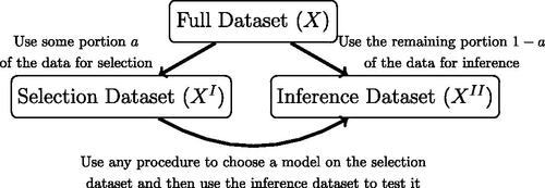
We primarily focus on demonstrating the applicability of these ideas in the context of (potentially high-dimensional) model selection and post-selection inference. With data splitting, the analyst picks some fraction $a\in \{\frac{1}{n},\dots ,\frac{n-1}{n},1\}$ of the data to use for model selection and the remaining $1-a$ fraction to use for inference as illustrated in Figure 1. Data fission is similar in spirit to this idea but instead uses randomization so that part of the information contained in every data point is used for both selection and inference. The procedure broadly works in three stages.

Fig. 1 Illustration of typical data splitting procedures for post-selection inference. Splitting the data has the advantage of allowing the user to choose any selection strategy for model selection, but at the cost of decreased power during the inference stage.

1. Split X into f(X) and g(X) such that $g(X)|f(X)$ is tractable to compute. The parameter τ controls the proportion of the information to be used for model selection.

2. Use f(X) to select a model and/or or hypotheses to test using any procedure available.

3. Use $g(X)|f(X)$ to test hypotheses and/or perform inference.

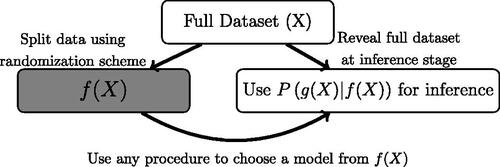
See Figure 2 for a graphical representation of the above steps. This approach can be viewed as a generalization of the methodologies discussed in Tian and Taylor (2018) and Rasines and Young (2022). In the above framework, these approaches amount to letting $f(X)=X+\gamma Z$ and g(X) = X with $Z\sim N(0,{\sigma }^2)$ for some fixed constant $\gamma >0$. In the case where $X\sim N(\mu ,{\sigma }^2)$ with known ${\sigma }^2$, the authors show that $g(X)|f(X)$ has a tractable finite sample distribution. In cases where X is non-Gaussian, however, $g(X)|f(X)$ is only described asymptotically. In the next section, we will explore alternative ways to construct g(X) that result in tractable finite sample distributions for non-Gaussian data.

Fig. 2 Illustration of the proposed data fission procedure. Similar to data splitting, it allows for any selection procedure for choosing the model. However, it achieves this through randomization rather than a direct splitting of the data.

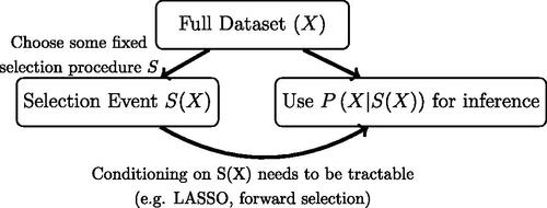
In some ways, these methodologies can be seen as a compromise between data splitting and the approach of data carving as introduced in Fithian, Sun, and Taylor (2014). Data carving, as illustrated in Figure 3, improves on data splitting in cases where the conditional distribution of the data given a selection event is known by including the leftover portion of Fisher information that was not used to inform the model choice in the inference procedure. A key limitation of this approach, however, is that it confines the analyst to model selection techniques with tractable post-selective distributions, such as the LASSO as described by Lee et al. (2016) or more general sequential regression procedures such as those discussed in Tibshirani et al. (2016). In many settings, ad-hoc exploratory data analyses such as the plotting of data or removal of outliers are ubiquitous and make data carving intractable.

Fig. 3 Illustration of data carving procedure as discussed in Fithian, Sun, and Taylor (2014). Data carving has the advantage of using all unused information for inference, but requires the selection procedure to be fixed at the onset of investigation. Moreover, computing the conditional distribution needs to be tractable, either in closed form (e.g., LASSO as described in Lee et al. 2016) or through numerical simulation. Thus, data carving and fission have complementary benefits and tradeoffs.

Although data fission conditions on f(X) rather than the selection event itself, it retains some similarities to data carving insofar as it uses a portion of every data point to inform both selection and inference. This has advantages relative to data splitting in at least two distinct ways. First, certain settings that involve sparse or rarely occurring features may result in a handful of data points having a disproportionate amount of influence—data fission allows for the analyst to “hedge their bets” by including these points in both the selection and inference steps. Second, in settings where the selected model is defined relative to a set of fixed covariates, the theoretical justification for data splitting becomes less clear conceptually. (In a fixed-X setup, how can a model that has been selected based on its ability to estimate the conditional distribution $Y\mid X^{\text{firsthalf}}$ also be understood to model the distribution that conditions on the other half of the split dataset $Y\mid X^{\text{secondhalf}}$?) For example, consider a time series dataset, where splitting a sample may require the analyst to have a selection and inference dataset that span entirely different time periods, or graph data where there is only one observation available for each location on a graph. On the other hand, similar to data splitting, data fission affords the analyst complete flexibility in how they choose their model based on the information revealed in the selection stage. In particular, the procedure can accommodate a model selection process that relies on qualitative or heuristic methods such as visual examination of residual plots or the consultation of domain experts to determine plausibility of the discovered relationships.

Although we anticipate that these ideas may have other downstream applications beyond selective inference such as data privacy (including differential privacy), creation of fake (synthetic) datasets, and comparing machine learning algorithms, these require new techniques that are out of the scope of the current work.

1.2 Related Work on Data Splitting and Carving

Our work is influenced by the existing literature on procedures for selective inference after model selection. Although data splitting is perhaps the oldest and most commonly used method for ensuring valid coverage guarantees after model selection, rigorous examination of data splitting has only recently emerged in the literature. Rinaldo, Wasserman, and G’Sell (2019) is one such example where the authors examine data splitting in an assumption-lean context.

Previously, the idea of adding and subtracting Gaussian noise has been employed for various goals in the literature. Tian and Taylor (2018) use this method for selective inference by introducing a noise variable that is independent of the original data, and involve it at various stages of the selection procedure (e.g., introducing perturbations to the gradient when using LASSO to select features). An alternative route for selective inference in Gaussian regression that is explored in Xing, Zhao, and Liu (2021) is to leave the response data unperturbed but create randomized versions of the covariates (termed “Gaussian mirrors”) by adding and subtracting Gaussian noise. This allows the authors to create test statistics with symmetric distributions under the null, enabling FDR control for the LASSO in high-dimensional settings. In contrast to both of these approaches, we focus on creating a perturbed version of the response that allows the analyst to conduct hypothesis selection in an arbitrary and heuristic fashion, as opposed to relying on a specific selection procedure such as the LASSO.

Randomization was also used in Li and Fithian (2021) to recast the knockoff procedure of Barber and Candès (2015) as a selective inference procedure for the linear Gaussian model that adds noise to the OLS estimates ($\widehat{\beta }$) to create a “whitened” version of $\widehat{\beta }$ to use for hypothesis selection. The work of Sarkar and Tang (2021) explores similar ways of using knockoffs to split $\widehat{\beta }$ into independent pieces for hypothesis selection but uses a deterministic splitting procedure. Although conceptually quite similar to our approach, these methods focus on splitting the coefficient estimates for a fixed model into two independent pieces and then adaptively choosing the hypotheses to test during the inference stage. As such, it is most naturally applied in low dimensional settings where model selection is less necessary. Similar randomization schemes for Gaussian distributed data are also explored in Ignatiadis et al. (2021) but are used for empirical Bayes procedures and not selective inference.

Outline of the article

The general methodology for data fission is introduced in Section 2. We illustrate how the procedure is used in the context of Gaussian data but then generalize this for the broader class of distributions where the data has a known conjugate prior. Examples are given across a variety of distributions commonly used for regression and data analysis such as Gaussian, Poisson, and Binomial. The remainder of the article explores the use of data fission for four different applications: selective CIs after interactive multiple testing in Section 3, fixed-design linear regression in Section 4, fixed-design generalized linear models in Section 5, and trend filtering in Section 6. Proofs for all theoretical results are omitted from the main body but included in Appendix B.

A key limitation within all of these applications—shared by much of classical statistics and conditional inference—is that theoretical guarantees can only be given under correct specification of the distribution of errors due to the need to ensure that the post-selective distribution is known and tractable. However, these guarantees are still assumption-lean in the sense of assuming an unknown form for the conditional mean μ. Situations where the variance is unknown and is estimated before data fission in the Gaussian case are discussed in low dimensional settings, but we leave theoretical guarantees in higher dimensions as an open avenue for future investigation. We provide some concluding remarks in Section 7.

2 Techniques to Accomplish Data Fission

With statistical inference in mind, we explore decompositions of X to f(X) and g(X) such that both parts contain information about a parameter θ of interest, and there exists some function h such that $X=h(f(X),g(X))$, and with either of the following two properties:

(P1).f(X) and g(X) are independent with known distributions (up to the unknown θ); or

(P2).f(X) has a known marginal distribution and g(X) has a known conditional distribution given f(X) (up to knowledge of θ).

The former property implies the latter, but the latter is generally more tractable. We explore alternative formulations that require weaker assumptions in Section 5.

2.1 Achieving (P2) Using “Conjugate Prior Reversal”

Suppose X follows a distribution that is a conjugate prior distribution of the parameter in some likelihood. We then construct a new random variable Z following that likelihood (with the parameter being X). Letting f(X) = Z and g(X) = X, the conditional distribution of $g(X)\mid f(X)$ will have the same form as X (with a different parameter depending on the value of f(X)). For example, suppose $X\sim \hspace{0.17em}\mathrm{Exp}\hspace{0.17em}(\theta )$, which is conjugate prior to the Poisson distribution. Thus, we draw $Z=(Z_1,\dots ,Z_B)$ where each element is iid $Z_i\sim \text{Poi}(X)$ and $B\in \{1,2,\dots \}$ is a tuning parameter. Let $f(X)=Z$ and g(X) = X. Then, the conditional distribution of $g(X)\mid f(X)$ is $\text{Gamma}(1+{\sum }_{i=1}^B{f}_i(X),\theta +B)$ On the other hand, $f(X)\sim \text{Geo}\left(\frac{\theta }{\theta +B}\right)$. Larger B results in a more informative f(X). More examples of such decompositions, which we term “conjugate prior reversal”, are in Appendix A. One drawback of this approach, however, is that it will often result in a distribution that is no longer straightforwardly related to the original parameter of interest and so extra care needs to be taken when performing inference—we explore this implication in greater detail in Section 5.

For exponential family distributions, we can construct f(X) and g(X) as follows.

Theorem 1.

Suppose that for some $A(·,·),{\theta }_1,{\theta }_2,H(·,·)$, the density of X is given by (1) $$p(x\mid {\theta }_1,{\theta }_2)=H({\theta }_1,{\theta }_2)\hspace{0.17em}\exp \hspace{0.17em}\{{\theta }_1^{T}x-{\theta }_2^{T}A(x)\}.$$(1)

Suppose also that we can find $h(·),T(·)$ and θ₃ such that (2) $$p(z\mid x,{\theta }_3)=h(z)\hspace{0.17em}\exp \hspace{0.17em}\{x^{T}T(z)-{\theta }_3^{T}A(x)\}$$(2) is a well-defined distribution. First, draw $Z\sim p(z|X)$, and let $f(X):=Z$ and $g(X):=X$. Then, $(f(X),g(X))$ satisfy the data fission property (P2). Specifically, note that f(X) has a known marginal distribution $p(z|{\theta }_1,{\theta }_2,{\theta }_3)=h(z)\frac{H({\theta }_1,{\theta }_2)}{H({\theta }_1+T(z),{\theta }_2+{\theta }_3)}$, while g(X) has a known conditional distribution given f(X), which is $p(x\mid z,{\theta }_1,{\theta }_2,{\theta }_3)=p(x\mid {\theta }_1+T(z),{\theta }_2+{\theta }_3)$.

Recall that all proofs are in Appendix B.

Remark 1

(Trading off information in f and g). As an extension to the above result, we can draw B samples independently from (2) denoted as Z_i for $i\in [B]$, in which case $f(X)=Z\equiv \{Z_1,\dots ,Z_B\}$ has marginal distribution $p(z|{\theta }_1,{\theta }_2,{\theta }_3)=\left[{\prod }_{i=1}^{B}h(z_i)\right]\frac{H({\theta }_1,{\theta }_2)}{H({\theta }_1+{\sum }_{i=1}^{n}T(z_i),{\theta }_2+B{\theta }_3)},$ and $g(X)=X$ has conditional distribution $p(x\mid z,{\theta }_1,{\theta }_2,{\theta }_3)=p(x\mid {\theta }_1+{\sum }_{i=1}^{B}T(z_i),{\theta }_2+B{\theta }_3).$ Larger B indicates more information in f(X), and thus less left over in g(X).

2.2 Example Decompositions

Below, we draw attention to techniques used in Sections 3, 4, 5, and 6.

• Gaussian. Suppose $X\sim N(\mu ,\Sigma )$ is d-dimensional ($d\ge 1$). Draw $Z\sim N(0,\Sigma )$. Then $f(X)=X+\tau Z$, where $\tau \in (0,\infty )$ is a tuning parameter, has distribution $N(\mu ,(1+{\tau }^2)\Sigma )$; and $g(X)=X-\frac{1}{\tau }Z$ has distribution $N(\mu ,(1+{\tau }^{-2})\Sigma )$; and $f(X)\perp \mathrm{}\mathrm{}\perp g(X)$. Larger τ indicates less informative f(X) (and more informative $g(X)\mid f(X)$).

• Bernoulli (P2). Suppose $X\sim \text{Ber}(\theta )$. Draw $Z\sim \text{Ber}(p)$ where $p\in (0,1)$ is a tuning parameter. Then $f(X)=X(1-Z)+(1-X)Z$ has marginal distribution $\text{Ber}(\theta +p-2p\theta )$; and g(X) = X has conditional distribution (given f(X)) as $\text{Ber}(\frac{\theta }{\theta +(1-\theta ){[p/(1-p)]}^{2f(X)-1}})$. Smaller p indicates more information in f(X).

• Poisson. Suppose $X\sim \text{Poi}(\mu )$. Fix parameter $p\in (0,1)$ and draw $Z \sim \text{Bin}(X,p)$. Then f(X) = Z has marginal distribution $\text{Poi}(p\mu )$; and $g(X)=X-Z$ is independent of f(X) and has distribution $\text{Poi}((1-p)\mu )$. Larger p indicates more informative f(X).

A larger (but still incomplete) list of decomposition strategies for specific distributions is available in Appendix A. We encourage the reader to consult this list in order to get a full appreciation for the applicability of this approach to disparate problems in statistics.

2.3 Relationship Between Data Splitting and Data Fission

We explore the conditions under which data fission yields estimators that are comparable to data splitting. Suppose we are given n iid observations $X=(X_1,\dots ,X_n)$, where $X_i\sim p(\theta )$. The data splitting approach chooses S as a random subset of $[n]$ of size a where $a\in \{\frac{1}{n},\dots ,\frac{n-1}{n},1\}$ is a tuning parameter. Letting ${\mathcal{I}}_X(\theta )$ denote the Fisher information for the complete sample and ${\mathcal{I}}_1(\theta )$ denote the Fisher information for a single observation, we then have $${\mathcal{I}}_X(\theta )=\underset{\text{Used for selection}}{\underbrace{an{\mathcal{I}}_1(\theta )}}+\underset{\text{Used for inference}}{\underbrace{(1-an){\mathcal{I}}_1(\theta )}}.$$

For data fission, note the following identity for smooth parametric models: ${\nabla }^2\mathcal{l}(\theta |X)={\nabla }^2\mathcal{l}(\theta ;f(X))+{\nabla }^2\mathcal{l}(\theta ;g(X)\mid f(X))$. Taking expectations, and denoting ${\mathcal{I}}_{f(X)},{\mathcal{I}}_{g(X)|f(X)}$ as the Fisher information for the selection and inference datasets yields $$\begin{array}{c}{\mathcal{I}}_X(\theta )={\mathcal{I}}_{f(X)}(\theta )+\mathbb{E}[-{\nabla }^2\mathcal{l}(\theta ;g(X)\mid f(X)]\\ ={\mathcal{I}}_{f(X)}(\theta )+\mathbb{E}\left[-\mathbb{E}[{\nabla }^2\mathcal{l}(\theta ;g(X)\mid f(X))\mid f(X)]\right]\\ =\underset{\text{for selection}}{\underbrace{{\mathcal{I}}_{f(X)}(\theta )}}+\underset{\text{for inference}}{\underbrace{\mathbb{E}[{\mathcal{I}}_{g(X)|f(X)}(\theta )]}}.\end{array}$$

For a fixed parameter a in data splitting, one can choose τ such that $\mathbb{E}[{\mathcal{I}}_{g(X)|f(X)}(\theta )]=(1-an){\mathcal{I}}_1(\theta )$ to find a comparable information split for data fission. This selected τ will only guarantee that the inference datasets created by data splitting and data fission approach contain the same information in expectation. For any particular realization of the fission step, ${\mathcal{I}}_{g(X)|f(X)}$ may be different than $(1-an){\mathcal{I}}_1(\theta )$. In situations where g(X) and f(X) are independent, this equality can be modified to hold exactly since $\mathbb{E}[{\mathcal{I}}_{g(X)|f(X)}(\theta )]={\mathcal{I}}_{g(X)}$.

Remark 2

(Trading information between f and g, part II). In the list of decompositions and in Remark 1 we noted that we could trade off “information” between f(X) and g(X) by varying certain hyperparameters. We can now clarify what this means. For a hyperparameter $p\in (a,b)$, we say that larger p corresponds to more informative f(X) and less informative $g(X)|f(X)$ to mean that $\underset{p\to b}{\lim }{\mathcal{I}}_{f(X)}(\theta )={\mathcal{I}}_X(\theta ) \text{and} \underset{\mathrm{p}\to \mathrm{b}}{\lim }\mathbb{E}[{\mathcal{I}}_{\mathrm{g}(\mathrm{X})\text{|f}(\mathrm{X})}(\theta )]\text{=0}.$

We now elaborate on the informal assertion in Section 1 that data fission for Gaussian data can be viewed as a continuous analog of data splitting with two examples.

Example 1

(Gaussian Datasets). Let ${\left\{X_i\right\}}_{i=1}^n$ be iid $N(\theta ,{\sigma }^2)$. ${\mathcal{I}}_1=\frac{1}{{\sigma }^2}$ and so $\frac{an}{{\sigma }^2}$ is the amount of information used for selection under a data splitting rule. If the data is fissioned using the rule in Section 2.2, then ${\mathcal{I}}_{f(X)}=\frac{n}{{\sigma }^2(1+{\tau }^2)}$. To compare the approaches, we note that the relation $a=\frac{1}{1+{\tau }^2}$ results in the same split of information.

Example 2

(Poisson Datasets). Let ${\left\{X_i\right\}}_{i=1}^n$ be iid $\text{Pois}(\mu )$. We have that ${\mathcal{I}}_1=\frac{1}{\mu }$ and so $\frac{an}{\mu }$ is the amount of information used for selection under a data splitting rule. If the data is fissioned using the rule described in Section 2.2, then ${\mathcal{I}}_{f(X)}=\frac{np}{\mu }$. The relation that equates the amount of information between data splitting and fission is then a = p.

The above examples are simplified because each data point is identically distributed so that each data point contains equivalent amounts of information about the unknown parameter θ. This symmetry allowed us to find a relation between a and τ that did not depend on the unknown parameters of interest. When the information value of data points varies, the two methods are not as directly comparable

Information splitting with non-identically distributed data

Consider a setting where data is independent but not identically distributed so each data point has different amounts of information. For instance, consider $Y_i\stackrel{\text{iid}}{\sim }N(\mu ,{\sigma }_i^2)$. Or consider the linear model where $Y_i\stackrel{\text{iid}}{\sim }N(x_i^T\beta ,{\sigma }^2)$ for $x_i\in {\mathbb{R}}^p$. In this case, ${\mathcal{I}}_{Y_i}(\beta )={\sigma }^2{x}_i{x}_i^T$, which places greater value on points with higher leverage. More generically, assume that $Y:=(Y_1,\dots ,Y_n)$ with ${\mathcal{I}}_{Y_i}(\theta )$ denoting the Fisher information for observation Y_i about a parameter θ. Consider m different ways of allocating the information for a fixed a which chooses an points for the first dataset and the remaining $1-an$ points for the second. Denote these hypothetical splits as $S_1,\dots ,S_m$, where $S_j\subseteq [n]$ refers to the indices that have been allocated to the first dataset. Let S denote the random variable that randomly selects S_j with probability p_j. For any j, we let ${\mathcal{I}}_{S_j}(\theta )=\sum _{i\in S_j}{\mathcal{I}}_{x_j}(\theta )$ denote the information allocated to the first dataset and ${\mathcal{I}}_{S_j^c}(\theta )=\sum _{i\in S_j^c}{\mathcal{I}}_{Y_i}(\theta )$ denote the information allocated to the second dataset.

In what follows, we let $m=(\begin{array}{c}n\\ an\end{array})$ and let $S_1,\dots ,S_m$ denote all possible ways of choosing an data points for the first dataset. We will also make the simplifying assumption that each $p_j=\frac{1}{(\begin{array}{c}n\\ an\end{array})}$ so that all possible splits have the same probability of being selected. Following Examples 1 and 2, suppose we try to create a comparable split of the information using data fission by choosing a fixed a and then picking τ such that ${\mathcal{I}}_{f(X)}=a{\sum }_{i=1}^n{\mathcal{I}}_{Y_i}(\theta )$. In this framework, this will also equate ${\mathcal{I}}_{f(X)}=\mathbb{E}\left[{\mathcal{I}}_S(\theta )\right]$ because $$\begin{array}{c}{\mathcal{I}}_{f(X)}=a\sum _{i=1}^n{\mathcal{I}}_{Y_i}(\theta )=\frac{1}{\left(\begin{array}{c}n\\ an\end{array}\right)}\sum _{i=1}^{\left(\begin{array}{c}n\\ an\end{array}\right)}a\sum _{j=1}^n{\mathcal{I}}_{Y_j}(\theta )\\ =\frac{1}{\left(\begin{array}{c}n\\ an\end{array}\right)}\sum _{i=1}^{\left(\begin{array}{c}n\\ an\end{array}\right)}\sum _{j=1}^n{\mathbb{1}}_{i\in S_i}{\mathcal{I}}_{Y_j}(\theta )=\mathbb{E}\left[{\mathcal{I}}_S(\theta )\right].\end{array}$$

Proposition 1 of Rasines and Young (2022), which we restate here with some adjustments to account for our setting, demonstrates that there is a sense in which the information split using fission is more efficient even though we have chosen τ such that it has the same expected information content as our data splitting procedure.

Fact 1 (Proposition 1 of Rasines and Young (2022)). Let $S_1,\dots ,S_m$ be deterministic data splitting rules and S be the random variable which returns a particular split S_j with some probability p_j such that ${\sum }_{i=1}^m{p}_i=1$. Suppose that data fission is conducted such that ${\mathcal{I}}_{f(X)}(\theta )=\mathbb{E}\left[{\mathcal{I}}_S\right]$. Assume that all information matrices ${\mathcal{I}}_{f(Y)}(\theta ),\mathbb{E}[{\mathcal{I}}_{g(Y)|f(Y)}(\theta )]$, and ${\mathcal{I}}_{Y_i}(\theta )$ are invertible and have dimension p × p. Let $\varphi$ be a real-valued, convex, and strictly increasing function function defined on the set of p × p positive definite matrices. Then $\varphi \left[{\mathcal{I}}_{f(Y)}{(\theta )}^{-1}\right]\le \mathbb{E}\left[\varphi ({\mathcal{I}}_S{(\theta )}^{-1})\right]$. Furthermore, when g(Y) is independent of f(Y), $\varphi \left[{\mathcal{I}}_{g(Y)}{(\theta )}^{-1}\right]\le \mathbb{E}\left[\varphi ({\mathcal{I}}_{S^c}{(\theta )}^{-1})\right]$.

Intuitively, data fission is more efficient because it splits the information in a determinsitic way, but data splitting introduces randomization into the splitting process which decreases efficiency. Since the width of confidence intervals for MLE parameters is a function of the inverse Fisher information, an immediate consequence of this is that MLE parameters constructed from data fission will have, on average, tighter confidence intervals compared with a data splitting rule with the same expected information split. Note that in the case where the same amount of information is available at each data point (i.e., ${\mathcal{I}}_{x_i}(\theta )={\mathcal{I}}_{x_j}(\theta )$ for all i, j), the above inequality becomes an equality and $\varphi \left[{\mathcal{I}}_{f(X)}{(\theta )}^{-1}\right]=\mathbb{E}\left[\varphi ({\mathcal{I}}_S{(\theta )}^{-1})\right]$. Therefore, in Examples 1 and 2, there is no apparent advantage to data splitting compared to data fission. When the information at each point varies, however, data fission can offer substantial benefits, which we explore in greater detail in Section 4.

3 Application: Selective CIs After Interactive Multiple Testing

Suppose we observe $y_i\sim N({\mu }_i,{\sigma }^2)$ for n data points with known ${\sigma }^2$ alongside generic covariates $x_i\in \mathcal{X}$. First, the analyst wishes to choose a subset of hypotheses $\mathcal{R}$ to reject from the set $\{H_{0,i}:{\mu }_i=0\}$ while controlling the false discovery rate (FDR), which is defined as the expected value of the $\text{false discovery proportion }(\text{FDP}):=\frac{|x_i\in \mathcal{R}:{\mu }_i=0|}{\max \left\{\right|\mathcal{R}|,1\}}$. After selecting these hypotheses, the analyst then may wish to construct either:

• multiple confidence intervals (CIs) with $1-\alpha$ coverage of μ_i for each $i\in \mathcal{R}$; or

• a single CI with $1-\alpha$ coverage of $\overline{\mu }=\frac{1}{\left|\mathcal{R}\right|}\sum _{i\in \mathcal{R}}{\mu }_i$.

One method for rejecting hypotheses and constructing CIs that achieve coverage for the individual μ_i would be using the BH procedure (Benjamini and Hochberg 1995) to form the rejection set and then construct CIs as described by Benjamini and Yekutieli (2005). In this problem, these would be calculated as $y_i\pm z_{\beta /2}$ where $\beta =\frac{\left|\mathcal{R}\right|\alpha }{n}$. However, we know of no methodology for aggregating the individual CIs to form a single CI that will cover $\overline{\mu }$.

An alternative approach for selective inference is to compute a p-value for testing each y_i, and then mask the p-value as proposed by the AdaPT (Lei and Fithian 2018) and STAR (Lei, Ramdas, and Fithian 2020) procedures. These interactive methods allow the data analyst to iteratively build a rejection set in a data adaptive way. A drawback of these approaches, however, is that they only are designed to work with a p-value. In contrast to the BH procedure, there is no available method to cover either the individual signals μ_i or $\overline{\mu }$. Data fission offers one possible path forward:

1. Draw $z_i\sim N(0,{\sigma }^2)$ and let $f(y_i)=y_i+\tau z_i$ with $g(y_i)=y_i-\frac{1}{\tau }{z}_i$.

2. Use $f(y_i)$ to select a rejection set of suspected non-nulls using any desired error-control procedure (say AdaPT, STAR or BH).

3. After selecting hypotheses, we can form CIs to cover each ${\mu }_i\in \mathcal{R}$ with $1-\alpha$ coverage as $g(y_i)\pm z_{\alpha /2}\sigma \sqrt{1+\frac{1}{{\tau }^2}}$ or we can form a $1-\alpha$ CI to cover $\overline{\mu }$ as $\frac{\sum _{i\in \mathcal{R}}g(y_i)}{\left|\mathcal{R}\right|}\pm z_{\alpha /2}\sigma \sqrt{\frac{1+\frac{1}{{\tau }^2}}{\left|\mathcal{R}\right|}}$.

To illustrate this procedure, we repeat the experiments in Section 4.3 of Lei, Ramdas, and Fithian (2020) but with fissioned data. Specifically, we let the data be arranged on a grid with non-nulls arranged in a circle in the center with ${\mu }_i=2$ for each non-null and ${\mu }_i=0$ for each null. We then form a rejection set using the BH, AdaPT, and STAR procedures and compute confidence intervals for $\overline{\mu }$. 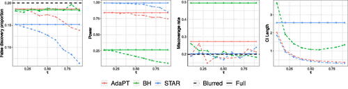Results are available in Figure 4. Fissioning the data allows the analyst to form CIs after forming a rejection set by varying τ, while post-selective CIs for non-fissioned data do not have proper coverage. For a more detailed discussion of the simulation and for additional demonstrations on Poisson data, consult Appendix E.

Fig. 4 Numerical results averaged over 250 trials for a $50\times 50$ grid of hypotheses with target FDR level chosen at 0.2 and τ varying over (0, 1). Solid lines denote metrics for the rejection sets formed using the full dataset and dotted lines denote metrics calculated using the rejection sets formed through data fission. All methods control FDR at the desired level, but “double dipping” to form CIs after forming a rejection set data results in invalid coverage. Fissioned CIs have the correct coverage. The fissiones CI lengths decrease as τ increases because more of the dataset gets reserved for inference.

4 Application: Selective CIs in Fixed-Design Linear Regression

We now turn to applying data fission to fixed-design Gaussian linear regression. We expand on the discussion in Rasines and Young (2022), and later build on several results in this section in our treatment of trend filtering in Section 6. We assume that y_i is the dependent variable and $x_i\in {\mathbb{R}}^p$ is a nonrandom vector of p features for $i=1,\dots ,n$ samples. We denote $X={(x_1,\dots ,x_n)}^T$ as the model design matrix and $Y={(y_1,\dots ,y_n)}^T$ with: $$Y=\mu +ϵ\text{ with }ϵ={({ϵ}_1,\dots ,{ϵ}_n)}^T\sim N(0,\Sigma ),$$ where $\mu =\mathbb{E}[Y|X]\in {\mathbb{R}}^n$ is a fixed unknown quantity and $ϵ\in {\mathbb{R}}^n$ is a random quantity with a known covariance matrix Σ (such as ${\sigma }^2{I}_n$ for known σ; we discuss unknown σ later).

During the fission phase, we introduce the independent quantities f(Y) and g(Y) created by adding Gaussian noise $Z\sim N(0,\Sigma )$ as described in Section 2.2, letting $f(Y)=Y+\tau Z$, and $g(Y)=Y-\frac{1}{\tau }Z$. We use f(Y) to select a model $M\subseteq [p]$ that, in turn, defines a model design matrix X_M which is a submatrix of X. After selecting M, we then use g(Y) for inference by fitting a linear regression on g(Y) against the selected covariates X_M.

Let $\widehat{\beta }$ (as a function of the chosen model M) be defined in the usual way as (3) $$\widehat{\beta }(M)=\underset{\tilde{\beta }}{\text{argmin}}{\Vert g(Y)-X_M\tilde{\beta }\Vert }^2={(X_M^T{X}_M)}^{-1}{X}_M^{T}g(Y).$$(3)

Note that we make no assumptions that $\mu =\mathbb{E}[Y|X]$ is guaranteed to be a linear combination of the chosen covariates. Our target parameter is therefore the best linear approximator of the regression function using the selected model (4) $${\beta }^{*}(M)=\underset{\tilde{\beta }}{\text{argmin}}\mathbb{E}\left[{\Vert Y-X_M\tilde{\beta }\Vert }^2\right]={(X_M^T{X}_M)}^{-1}{X}_M^T\mu .$$(4)

We are then able to form CIs that guarantee $1-\alpha$ coverage of ${\beta }^{*}(M)$ as follows.

Theorem 2.

For $\widehat{\beta }(M)$ from (3) and ${\beta }^{*}(M)$ from (4), we have $$\begin{array}{c}\widehat{\beta }(M)\sim N({\beta }^{*}(M),(1+{\tau }^{-2}){(X_M^T{X}_M)}^{-1}{X}_M^T\\ \Sigma X_M{(X_M^T{X}_M)}^{-1}).\end{array}$$

Furthermore, we can form a $1-\alpha$ CI for the kth element of ${\beta }^{*}(M)$ as $${\widehat{\beta }}^k(M)\pm z_{\alpha /2}\sqrt{(1+{\tau }^{-2}){\left[{(X_M^T{X}_M)}^{-1}{X}_M^T\Sigma X_M{(X_M^T{X}_M)}^{-1}\right]}_{kk}}.$$

An assumption of this procedure is that the variance is known in order to do the initial split between f(Y) and g(Y) during the fission phase. In the case of unknown variance, one can use an estimator $\widehat{\sigma }$ to create the split, but this forces the analyst to then condition on both f(Y) and $\widehat{\sigma }$, which may not have a tractable distribution in high dimensional settings. In the case where p is fixed and $n\to \infty$, we explore an extension of this methodology to account for unknown variance in Section B. Extending this approach to finite samples and high-dimensional regimes remains an open question for future lines of research.

A key advantage that data fission has over data splitting is that it allows the analyst to smoothly trade off information between selection and inference datasets by tuning τ, while data splitting forces the analyst to allocate points discretely to either the selection or inference datasets. When the sample size is large and the distribution of covariates is well behaved, data splitting may be able to tradeoff information relatively smoothly by changing the proportion of data points in each sample. However, data fission will outperform data splitting in settings with small sample size with a handful of points with high leverage. Data splitting has a disadvantage in this setting because the analyst is forced to choose to allocate each of these leverage points to either the selection or inference dataset. In contrast, data fission enables the analyst to “hedge their bets” so that a piece of the information contained in each leverage point is allocated to both the selection and inference datasets. Figure 5 offers an illustration of this tendency on an example dataset and an extended discussion on this topic can be found in Appendix C.

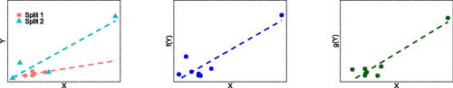
Fig. 5 Comparison of data splitting (left) and data fission (middle, right) for dataset with one highly influential point. Splitting the data and fitting a regression results in substantially different fitted models because the fitted values are heavily influenced by a single data point. In contrast, data fission keeps the same X location for every data point, but randomly perturbs the response Y with random noise to create new variables f(Y) and g(Y): notice the slight difference in the two figures. This enables the analyst to keep a “piece” of every data point in both f(Y) and g(Y), ensuring that leverage points have an impact in both copies of the dataset.

We now demonstrate the advantages that data fission has over data splitting through an empirical study. We conduct inference on some vector Y given a set of covariates X and a known covariance matrix $\Sigma ={\sigma }^2{I}_n$ as follows:

1. Decompose y_i into $f(y_i)=y_i-Z_i$ and $g(y_i)=y_i+Z_i$ where $Z_i\sim N(0,{\sigma }^2)$.

2. Fit $f(y_i)$ using LASSO to select features, denoted as $M\subseteq [p]$.¹

3. Fit $g(y_i)$ by linear regression without regularization using only the selected features

4. Construct CIs for the coefficients trained in step 3, each at level α, using Theorem 2.

Simulation setup

We choose ${\sigma }^2=1$ and generate n = 16 data points with p = 20 covariates. For the first 15 data points, we have an associated vector of covariates $x_i\in {\mathbb{R}}^p$ generated from independent Gaussians. The last data point, which we denote $x_{\text{lev}}$, is generated in such a way as to ensure it is likely to be more influential than the remaining observations due to having much larger leverage. We define $x_{\text{lev}}=\gamma (|X_1{|}_{\infty },\dots ,|X_p{|}_{\infty })$ where X_k denotes the the kth column vector of the model design matrix X formed from the first 15 data points and γ is a parameter that we will vary within these simulations that reflects the degree to which the last data point has higher leverage than the first set of data points. We then construct $y_i\sim N({\beta }^T{x}_i,{\sigma }^2)$. The parameter β is nonzero for 4 features: $({\beta }_1,{\beta }_{16},{\beta }_{17},{\beta }_{18})=S_{\Delta }(1,1,-1,1)$ where $S_{\Delta }$ encodes the signal strength. We use 500 repetitions and summarize performance as follows. For the selection stage, we compute the power (defined as $\frac{|j\in M:{\beta }_j\ne 0|}{|j\in [p]:{\beta }_j\ne 0|}$) and precision (defined as $\frac{|j\in M:{\beta }_j\ne 0|}{\left|M\right|}$) of selecting features with a nonzero parameter. For inference, we use the false coverage rate (defined as $\frac{|k\in M:{[{\beta }^{\star }(M)]}_k\notin {\text{CI}}_k|}{\max \left\{\right|M|,1\}}$) where ${\text{CI}}_k$ is the CI for ${[{\beta }^{\star }(M)]}_k$. We also track the average CI length within the selected model.

As an illustration, Figure 6 shows an instance of the selected features and corresponding CIs for an example trial run. As a point of comparison, we compare the CIs constructed using data fission with those constructed using data splitting (when 50% of the dataset is used for selection and the remaining for inference). We also compare these results to the (invalid) procedure where the original dependent variable is used twice to both select features and construct intervals The third methodology will not have coverage guarantees but it is still a useful point of comparison for evaluating the performance of the other two (valid) methodologies. Figure 7 shows results averaged over 500 trials. Data splitting and data fission both control the FCR, but data fission dominates data splitting across every other metric—including significantly tighter CIs and higher power and precision. In simulation studies with larger sample sizes and less skewed covariates, data fission and data splitting have comparable performance—see Appendix E for details.

Fig. 6 An instance of the selected feature (blue crosses) and the constructed CIs using fissioned data (left), full data twice (middle), and split data (right) with $S_{\Delta }=0.2$ and target FCR set at 0.2. The selected features are marked by blue crosses, which include all of the nonzero coefficients (corresponding to almost 100% power for selection) and also a few zero coefficients (corresponding to around 70% precision for selection). CIs which do not cover the parameters correctly are marked red.

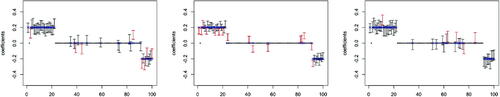
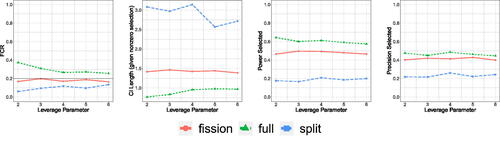
Fig. 7 FCR, average length of the CIs, and power/precision for the selected features, when varying the leverage parameter γ in $\{2,3,4,5,6\}$. The results are averaged over 500 trials. Both data splitting and data fission still control FCR, but data fission now has higher power and precision, as well as tighter CIs than data splitting.

5 Application to Selective CIs in Fixed-Design Generalized Linear Models and Other Quasi-MLE Problems

For regression problems involving non-Gaussian distributed data, the same generic principle can be used as in Section 4. If the underlying distribution of Y is known up to a set of unknown parameters and aligns with one of the distributions described in Appendix A, we can fission the data and then use f(Y) for selection, while reserving $g(Y)|f(Y)$ to conduct inference. Even in cases where we are certain that the distribution of Y has been properly specified and the fission procedure is valid, it is important to construct CIs that are robust to model misspecification for two reasons. First, because it is unlikely in practical settings that we are going to be able to select a set of covariates that corresponds to the “actual” conditional mean of the data. Second, the post-selective distribution $f(Y)|g(Y)$ may be ill-behaved and difficult to work with even if Y is easy to model. For example, if $Y\sim \text{Ber}(\theta )$, the post-selective distribution $g(Y)|f(Y)$ constructed from Section 4 is $\text{Ber}(\frac{\theta }{\theta +(1-\theta ){[p/(1-p)]}^{2f(Y)-1}})$. Maximizing this likelihood function will be challenging since the likelihood is non-convex, so it may be practical to model the likelihood as a probit or logistic model as a working assumption.

This approach of using maximum likelihood estimation to train a model but to construct guarantees in an assumption-lean setting is termed quasi-maximum likelihood estimation (QMLE). Most work in this setting, such as Buja et al. (2019), and Rinaldo, Wasserman, and G’Sell (2019), are designed around a background assumption where both the covariates and response are treated as iid random variables. Such theory is inapplicable to data fission since the covariates are observed during the model selection stage and therefore inference on g(Y) is only valid if both X and f(Y) are conditioned on. Fahrmeir (1990), however, works in the setting of non-identically distributed but independent data with fixed covariates and therefore can be applied to this setting. We first recap the relevant theory and then apply it to data fission when used for forming post-selective CIs in GLMs.

5.1 Problem Setup and a Recap of QMLE Methods

Suppose we observe n independent random observations $y_i\in \mathbb{R}$ alongside fixed covariates $x_i\in {\mathbb{R}}^p$ and that we fission each data point such that the below assumption holds.

Assumption 1.

Data fission is conducted such that $g(y_i)\perp \mathrm{}\mathrm{}\perp g(y_k)$ $|f(Y),X$ for all $i\ne k$.

This is a different condition compared to the rules described in Section 1. Any fissioning rule which satisfies (P1) would also satisfy this (weaker) condition. The majority of decompositions in Appendix A following $(\mathbf{P}\mathbf{2})$ also satisfy Assumption 1 but this is not necessarily the case—for instance, the third rule for fissioning Gaussian distributed data would result in a post-selective distribution that is tractable but with correlated entries. However, if a fissioning process exists that creates independent entries in $g(Y)|f(Y),X$, the procedures outlined in this section will apply.

During model selection, a model $M\subseteq [p]$ is chosen from f(Y) which result in an annealed set of covariates ${\tilde{x}}_i\in {\mathbb{R}}^{\left|M\right|}$ and model design matrix X_M. We then find an estimate for β using a working model of the density for $g(y_i)|f(Y),X$ as $p(g(y_i)|\beta ,f(Y),X_M)$, which defines the quasi-likelihood function $L_n(\beta ):={\sum }_{i=1}^n\hspace{0.17em}\log \hspace{0.17em}p(g(y_i)|\beta ,f(Y),X_M)$. Denote the score function $s_n(\beta )=\frac{\partial L_n}{\partial \beta }$ as well as the quantities $H_n(\beta )=-\frac{{\partial }^2{L}_n}{\partial \beta {\beta }^T}$, and $V_n(\beta )=\text{var}(s_n(\beta ))$. If $\mathbb{E}(H_n(\beta ))$ is positive definite, the target parameter ${\beta }^{\star }(M)$ is the root of $E(s_n(\beta ))$ which is also the parameter which minimizes the KL distance between the true distribution (denoted as $q(g(y_i|f(Y),X)$) and the working model because $$\begin{array}{c}{\beta }_n^{\star }(M)=\underset{\beta }{\text{argmin}}\mathbb{E}\left(\hspace{0.17em}\log \hspace{0.17em}q(g(y_i)|X,f(Y))-L_n(\beta )\right)\\ =\underset{\beta }{\text{argmin}}{\mathrm{D}}_{KL}\left(\prod _{i=1}^{n}q(g(y_i)|X,f(Y))||\prod _{i=1}^{n}p(g(y_i)|\beta ,f(Y),X_M)\right).\end{array}$$

We define ${\widehat{\beta }}_n(M)$ as the quasi-likelihood maximizer. Under mild regularity conditions, ${\widehat{\beta }}_n(M)$ behaves asymptotically like $N({\beta }^{\star }(M),H_n^{-1}({\beta }_n^{\star }(M))V_n({\beta }_n^{\star }(M))H_n^{-1}({\beta }_n^{\star }(M)))$. Plug-in estimates ${\widehat{H}}_n:=H_n({\widehat{\beta }}_n(M))$ and ${\widehat{V}}_n:=s_n({\widehat{\beta }}_n(M))s_n{({\widehat{\beta }}_n(M))}^T$ will yield asymptotically conservative estimates for the covariance matrix, allowing the user to form confidence intervals. For a detailed technical account, see Appendix B.

5.2 Simulation Results

We verify the efficacy of this procedure through an empirical simulation. The advantages of data fission are again most apparent in settings with relatively few data points and a handful of leverage points just as we saw in the Gaussian case in Section 4.

Simulation setup

Let y_i be the dependent variable with $y_i\sim \text{Pois}(\hspace{0.17em}\exp \hspace{0.17em}\left\{{\beta }^T{x}_i\right\})$ where $x_i\in {\mathbb{R}}^p$ is a vector of p features. We generate n = 16 data points with p = 20 covariates, where the parameter β is nonzero for 4 features: $({\beta }_1,{\beta }_{16},\dots ,{\beta }_{19})=S_{\Delta }(1,1,-1,1)$ and $S_{\Delta }$ encodes the signal strength. For the first 15 observations, $x_i\in {\{0,1\}}^2\times {\mathbb{R}}^{18}$, where the first two follow $\text{Ber}(1/2)$ and the rest follow independent standard Gaussians. The last data point, which we again denote $x_{\text{lev}}=\gamma (|X_1{|}_{\infty },\dots ,|X_p{|}_{\infty })$ where X_k denotes the the kth column vector of the model design matrix X formed from the first 15 data points and γ is the leverage parameter. Our proposed procedure is

1. Decompose each y_i as $f(y_i)\sim \text{Bin}(y_i,p)$, and $g(y_i)=y_i-f(y_i)$.

2. Fit $f(y_i)$ by the GLM with log-link and LASSO regularization to select $M\in [p]$.

3. Fit $g(y_i)$ by another GLM without regularization with log-link using only the selected features and an offset of $\hspace{0.17em}\log \hspace{0.17em}(1-p)$ to account for the effect of the randomization.

4. Construct CIs for the coefficients trained in the third step, each at level α and with the standard errors estimated as in Theorem 4 in the Appendix. For the experiments shown below, we also apply a finite sample correction as described in Pustejovsky and Tipton (2018).

Since step 2 may not select the correct model, the CIs in step 4 cover ${\beta }_n^{\star }(M)$.

Results are shown in Figure 8. Model performance metrics are the same as those used in Section 4 with ${\beta }_n^{\star }(M)$ replacing ${\beta }^{\star }(M)$. The CIs for the non-fission approaches (data splitting and full data twice) are also constructed using sandwich estimators of the variance corresponding to Theorem 4 in the Appendix. Every method controls the FCR empirically, but the CI lengths for data fission are significantly tighter than for data splitting. Data fission is also more powerful at the selection stage than data splitting. Results for higher n settings as well as when this general framework is applied to logistic regression are contained in Appendix E. Across all of these cases, using the full dataset twice no longer results in FCR control, as expected.

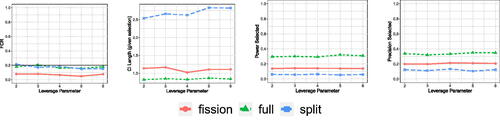
Fig. 8 FCR, length of the CIs, FSR, power for the sign of parameters, and power and precision for the selected features, when varying the leverage parameter α in $\{2,3,4,5,6\}$ for Poisson data over 500 trials. CIs constructed using data fission are tighter than data splitting, and power during the selection stage is higher.

6 Application to Post-Selection Inference for Trend Filtering and Other Nonparametric Regression Problems

Consider a nonparametric setup with y_i and covariates x_i following $y_i=f_0(x_i)+{ϵ}_i$, where f₀ is the underlying function to be estimated and ϵ_i is random noise. We denote $Y={(y_1,\dots ,y_n)}^T$ and $ϵ={({ϵ}_1,\dots ,{ϵ}_n)}^T$. For now, assume that $ϵ\sim N(0,\Sigma )$ for some known Σ. We can apply the methodologies of Sections 2.2 and 4 to this problem as follows:

1. Decompose Y into $f(Y)=Y+\tau Z$ and $g(Y)=Y-\frac{1}{\tau }Z$ where $Z\sim N(0,\Sigma )$.

2. Use f(X) to choose a basis $a_1,\dots ,a_p$ for the series expansion of x_i and denote $a(x_i)={(a_1(x_i),\dots ,a_p(x_i))}^T$. Let A denote the matrix of basis vectors for all n data points.

3. Use $g(X)|f(X)$ to construct pointwise or uniform CIs as described below.

Pointwise CI

We first note that the fitted line (5) $$\widehat{\beta }(A)=\underset{\beta }{\text{argmin}}{\Vert g(Y)-A\beta \Vert }^2={(A^{T}A)}^{-1}{A}^{T}g(Y)$$(5) corresponds to $A\widehat{\beta }(A)$ which is just the projection of g(Y) onto the basis chosen during the model selection stage. Meanwhile, we define the projected regression function as (6) $${\beta }^{*}(A)=\underset{\beta }{\text{argmin}}\mathbb{E}\left[{\Vert Y-A\beta \Vert }^2\right]={(A^{T}A)}^{-1}{A}^T{f}_0(X).$$(6)

We are then interested in using the fitted estimates ${\widehat{\mu }}_{x_i}(A)=a{(x_i)}^T\widehat{\beta }(A)$ to construct intervals that guarantee coverage for the underlying function $f_0(x_i)$ projected onto the chosen basis which we denote as ${\mu }_{x_i}^{*}(A)=a{(x_i)}^T{\beta }^{*}(A)$ and refer to as the projected mean.

Corollary 1.

Recall the definitions of $y_i,{ϵ}_i,\widehat{\beta }(A),{\beta }^{*}(A)$ from (5) and (6). When ϵ has known variance Σ, ${\widehat{\mu }}_{x_i}(A)\sim N({\mu }_{x_i}^{*}(A),(1+{\tau }^{-2})a{(x_i)}^T{(A^{T}A)}^{-1}{A}^T\Sigma A{(A\prime A)}^{-1}$ $a(x_i))$ and a $1-\alpha$ CI for ${\mu }_{x_i}^{*}(A)$ is ${\widehat{\mu }}_{x_i}(A)\pm$ $z_{\alpha /2}\sqrt{(1+{\tau }^{-2})a{(x_i)}^T{(A^{T}A)}^{-1}{A}^T\Sigma A{(A^{T}A)}^{-1}a(x_i)}.$

Uniformly valid CIs

We can also construct uniformly valid CIs ${\left\{C{I}_i\right\}}_{i=1}^n$ to cover the projected mean, controlling the simultaneous Type I error rate defined as $\mathbb{P}(\exists i\in [n]:{\mu }_{x_i}^{*}(A)\notin {\text{CI}}_i).$ Here, we further assume homoscedastic errors so $\Sigma ={\sigma }^2{I}_n$. Construct ${\text{CI}}_i:=({\widehat{\mu }}_{x_i}(A)-w,{\widehat{\mu }}_{x_i}(A)+w)$, where the width $w:=c(\alpha )·\sigma \sqrt{(1+{\tau }^{-2})a{(x_i)}^T{(A^{T}A)}^{-1}a(x_i)}$, where $c(\alpha )$ is a multiplier. By eq. (5.5) in Koenker (2011), $c(\alpha )$ is the solution to the equation $\frac{\left|\gamma \right|}{2\pi }{e}^{-c^2/2}+1-\Phi (c)=\alpha /2,$ where $\left|\gamma \right|={\sum }_{i=1}^{n-1}\left|\right|\tilde{a}(x_{i+1})-\tilde{a}(x_i)|{|}_2$ is the length of the curve connected by $\tilde{a}(x_i):=\frac{{(A^{T}A)}^{-1/2}a(x_i)}{\left|\right|{(A^{T}A)}^{-1/2}a(x_i)\left|\right|}$.

Fact 2. (Koenker 2011) The above constructed CIs will cover the projected mean uniformly: $\mathbb{P}(\exists i\in [n]:{\mu }_{x_i}^{*}(A)\notin {\text{CI}}_i)\le \alpha ,$ where ${\{{\mu }_{x_i}^{*}(A)\}}_{t=1}^n$ denotes the projected mean.

6.1 Application to Trend Filtering

We explore how this approach to nonparametric inference performs empirically through the lens of trend filtering as proposed by Kim et al. (2009) and Steidl, Didas, and Neumann (2006). Here, we consider the problem of estimating the underlying smooth trend of a time series $y_t\in \mathbb{R}$ with $t=1,\dots ,n$. We have the same equation as in the standard nonparametric setup, but with $x_i=t$ for all i and thus have that $y_t=f_0(t)+{ϵ}_t$. Our goal is to estimate the underlying trend $(f_0(1),\dots ,f_0(n))$. The approach of (first order) trend filtering is to fit a piecewise linear approximation to this data with adaptively chosen breakpoints or knots by solving: $\widehat{x}=\underset{x_t\in \mathbb{R}}{\text{argmin}}1/2{\sum }_{t=1}^n{(y_t-x_t)}^2+\lambda {\sum }_{t=2}^{n-1}|x_{t-1}-2x_t+x_{t+1}|.$ Although we focus on first order trend filtering, our methodology straightforwardly generalizes to higher order trend filtering. For a detailed overview of trend filtering, including generalization to higher order polynomials, see Appendix D.

An issue issue with trend filtering is that uncertainty quantification is not generally tractable since the knots are chosen adaptively. In some settings, data carving approaches may offer a viable path forward. When the (fused or generalized) lasso is used to select the choice of knots, methods such as Chen, Jewell, and Witten (2022), Duy and Takeuchi (2021), and Hyun, G’Sell, and Tibshirani (2018) can be used to construct tests and CIs with valid post-selective distributions. The drawback of these approaches is that they offer the analyst no flexibility during the selection stage. If the analyst wishes to change the degree of the fitted polynomial or decrease the number of chosen knots after seeing preliminary results, inferential guarantees are no longer available. Although such actions are common in applied data analysis, data carving approaches do not easily handle ad-hoc changes to the prespecified selection methodology. Data fission offers the analyst flexibility to change the amount of regularization (alter the number of knots) or change the degree of the trend filtered estimate after a preliminary view of the selected model performance.

Similar to Section 4, an assumption of known variance is required when using data fission in order to ensure the selection and inference datasets are independent. Approaches that estimate variance empirically are explored in Appendix E but we leave theoretical guarantees for future work. The proposed procedure is:

1. Decompose Y into $f(Y)=Y+\tau Z,g(Y)=Y-\frac{1}{\tau }Z$ where $Z\sim N(0,\Sigma )$.

2. Train a kth order trendfilter using f(Y) and select the tuning parameter λ by selecting the set of knots ${\left\{{\tau }_k\right\}}_{k\in 1}^m$ with the minimum cross-validation error.²

3. Construct a kth degree falling factorial basis, as described in Tibshirani (2014), with knots at ${\left\{{\tau }_k\right\}}_{k=1}^m$ and use this to regress against g(Y). Note that when k = 0 or k = 1, this reduces to generating the more familiar truncated power basis.

4. Get pointwise CIs for each data point $t=1,\dots ,n$ at level α as described in Theorem 1. In cases where $\Sigma ={\sigma }^2{I}_n$, we can also construct uniform CIs using Theorem 2.

Simulation setup

We verify the efficacy of this approach through an experiment. We simulate data as $y_t=f(t)+z_t$ for $t\in [n]$, where $z_t\sim N(0,{\sigma }^2)$, and $f_0(t)$ is generated by $f_0(t+1)=f_0(t)+v_t$. With probability $1-p$, we let $v_{t+1}=v_t$ (no slope change in the trend). With probability p, we choose $v_{t+1}$ from a uniform distribution on $[-0.5,0.5]$. We choose the initial slope $v_1\sim \text{Unif}[-0.5,0.5]$ and set $f_0(0)=0$.

We use the above procedure to select knots and conduct inference. An example of how this methodology performs when compared to the (invalid) approach of using the full dataset twice is shown in Figure 9 for pointwise CIs. As there is not an obvious way to apply data splitting to trend filtering, this view is excluded. Although using the full dataset twice is invalid, it performs worse for datasets that are more volatile, either in terms of the underlying structural trend (i.e., more knots and/or larger slopes) or in terms of the underlying noise level. For a similar demonstration with uniform CIs see Appendix E.

Fig. 9 Two instances of the observed points (in yellow) and the pointwise CIs (in blue if correctly cover the trend, in red if not; the time points with false coverage are also amplified in the bar at the bottom) using two types of methods: full data twice (left), and data fission (right). The underlying projected mean is marked in cyan, which mostly overlaps with the true underlying trend. The true knots are marked by vertical lines. Using data fission results in correct empirical coverage (the 0.225 above was for just one run, the average is below 0.2). In contrast, the FCR is not controlled when using the full dataset twice; it worsens as the underlying noise and trend become more volatile.

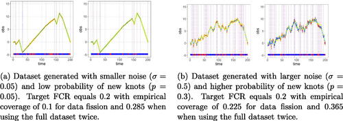
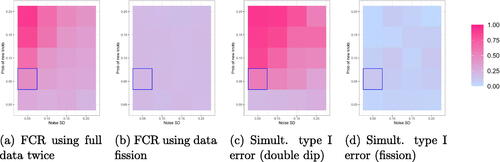
We repeat over 500 trials and report the results in Figure 10. Reusing the full dataset performs most comparably to data fission when the noise is small and the probability of new knots is low. For noisier data and more volatile trends, reusing the data results in anticonservative CIs. See Appendix E for more detailed empirical results.

Fig. 10 FCR for the pointwise CIs and simultaneous Type I error for uniform CIs when varying the probability of having knots p in $\{0.01,0.55,0.1,0.145,0.19\}$ and the noise SD in $\{0.05,0.1,0.15,0.2\}$ (the blue circled cell represents the setting for the first shown instance in Figure 9). The CIs generated using full data twice do not have valid FCR or simultaneous Type I error control, especially when p is large (more knots) and the noise standard deviation is small, but data fission is always valid.

6.2 Application to Spectroscopy

In Politsch et al. (2020), the authors introduce trend filtering as a tool for astronomical data analysis with spectral classification as a motivating example. In spectroscopy, we observe a spectrum consisting of wavelengths (λ) and corresponding measurements of the coadded flux ($f(\lambda )$). Trend filtering can then used to create a “spectral template”—a smoothed line of best fit for the observations. This template is combined with emission-line parameter estimates to classify the astronomical object. The authors demonstrate that trend filtering performs well empirically compared to the existing state-of-the-art for creating spectral templates which revolve around low-dimensional principal component analysis. We use this analysis as a way of demonstrating how CIs constructed using data fission appear for real data.

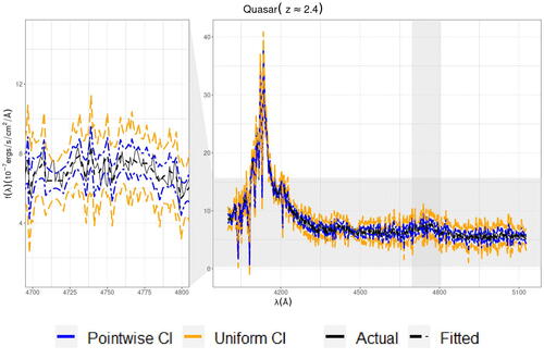
The dataset used for this analysis is the twelfth data release of the Baryon Oscillation Spectroscopic Survey (Alam et al. 2015). We estimate a spectral template using trend filtering, along with pointwise and uniform confidence bands (using the methods from Section 6) designed to cover the conditional mean $\mu =\mathbb{E}[f(\lambda )|\lambda ]$ of the observed spectra of the same three object discussed in Politsch et al. (2020). In this setting, the flux measurement variances are known a priori and account for the statistical uncertainty introduced by photon noise, CCD read noise, and sky-subtraction error. The results are shown in Figure 11 for the quasar³ and in Appendix F for the remaining objects. Since the confidence bands displayed are covering the conditional mean and not the observed data, there is no objective “ground truth” to compare the outputs of the model to in order to assess goodness of fit. Therefore, the results need to be judged holistically.

Fig. 11 Fitted values as well as uniform and pointwise CIs for a quasar object fit using linear trend filtering. The right view shows the trend filter over the entire spectrum, but the left view “zooms in” on a smaller subset of the data to aid in visual identification.

7 Conclusion

We have proposed a method for selective inference through external randomization that allows flexibility to choose models in an arbitrary and data dependent way, like in data splitting, but also provides a more efficient split of available information in some settings. We demonstrate the efficacy of these methods in four applications: effect size estimation after interactive multiple testing, Gaussian linear regression, generalized linear models, and trend filtering. In the case of linear regression and GLMs, we note tighter CIs and higher power compared to data splitting in settings with leverage points and small sample size. For trend filtering, data fission enables uncertainty quantification while offering flexibility in choosing the number of knots and degree of the polynomial based on heuristic criteria.

Numerous avenues for follow-up work exist. Although we note promising empirical results that suggest this procedure can be generalized to situations where the variance is unknown and the assumed distribution on the error term is misspecified, additional work needs to be done to establish rigorous guarantees, especially in high dimensional settings. Independently, it is possible to repeat the data fission procedure multiple times in parallel, but aggregating results seems nontrivial. Last, we anticipate applications to contemporary problems such as the creation of fake datasets and enabling differential privacy.

Supplementary Materials

Appendix A contains a list of additional decomposition rules for several commonly encountered distributions. Appendix B contains proofs of all deferred theoretical results as well as a more extensive discussion of asymptotics for QMLE methods. Appendix C contains an extended comparison between data splitting and data fission in the context of linear regression. Appendix D contains background information on trend filtering. Appendix E contains additional simulation results. Appendix F contains additional details on the spectroscopy example.

Disclosure Statement

The authors report there are no competing interests to declare.

Notes

1 In our experiments, we ue cv.glmnet in R package glmnet and choosing the tuning parameter λ by the 1 standard deviation rule, which can be found in the value of lambda.1se)

2 Although we restrict ourselves to a fixed selection rule for simulation purposes, data fission allows for the use of any arbitrary method of choosing the set of knots. For a discussion of alternative methods for choosing the tuning parameter λ, see Appendix E.

3 DR12, Plate = 7130, MJD =5659, Fiber = 58. Located at (RA,Dec, z) $\approx ({349.737}^{°},{33.414}^{°},2.399)$.

References

- Alam, S., Albareti, F. D., Prieto, C. A., Anders, F., Anderson, S. F., Anderton, T., Andrews, B. H., Armengaud, E., Aubourg, E., Bailey, S., and et al. (2015), “The Eleventh and Twelfth Data Releases of the Sloan Digital Sky Survey: Final Data from SDSS-III,” The Astrophysical Journal Supplement Series, 219. DOI: 10.1088/0067-0049/219/1/12.
- Barber, R. F., and Candès, E. J. (2015), “Controlling the False Discovery Rate via Knockoffs,” Annals of Statistics, 43, 2055–2085.
- Benjamini, Y., and Hochberg, Y. (1995), “Controlling the False Discovery Rate: A Practical and Powerful Approach to Multiple Testing,” Journal of the Royal Statistical Society, Series B, 57, 289–300. DOI: 10.1111/j.2517-6161.1995.tb02031.x.
- Benjamini, Y., and Yekutieli, D. (2005), “False Discovery Rate–Adjusted Multiple Confidence Intervals for Selected Parameters,” Journal of the American Statistical Association, 100, 71–81. DOI: 10.1198/016214504000001907.
- Buja, A., Brown, L., Kuchibhotla, A. K., Berk, R., George, E., and Zhao, L. (2019), “Models as Approximations II: A Model-Free Theory of Parametric Regression,” Statistical Science, 34, 545–565. DOI: 10.1214/18-STS694.
- Chen, Y., Jewell, S., and Witten, D. (2022), “More Powerful Selective Inference for the Graph Fused Lasso,” The Journal of Computational and Graphical Statistics, 32, 577–587. DOI: 10.1080/10618600.2022.2097246.
- Duy, V. N. L., and Takeuchi, I. (2021), “Parametric Programming Approach for More Powerful and General Lasso Selective Inference,” in Proceedings of The 24th International Conference on Artificial Intelligence and Statistics, Volume 130 of Proceedings of Machine Learning Research, eds. A. Banerjee and K. Fukumizu, pp. 901–909. PMLR.
- Fahrmeir, L. (1990), “Maximum Likelihood Estimation in Misspecified Generalized Linear Models,” Statistics, 21, 487–502.
- Fithian, W., Sun, D., and Taylor, J. (2014), “Optimal Inference after Model Selection,” arXiv:1410.2597.
- Hyun, S., G’Sell, M., and Tibshirani, R. J. (2018), “Exact Post-Selection Inference for the Generalized Lasso Path,” Electronic Journal of Statistics, 12, 1053–1097. DOI: 10.1214/17-EJS1363.
- Ignatiadis, N., Saha, S., Sun, D. L., and Muralidharan, O. (2021), “Empirical Bayes Mean Estimation with Nonparametric Errors via Order Statistic Regression on Replicated Data,” Journal of the American Statistical Association, 118, 987–999. DOI: 10.1080/01621459.2021.1967164.
- Kim, S.-J., Koh, K., Boyd, S., and Gorinevsky, D. (2009), l1 trend Filtering,” SIAM Review, 51, 339–360.
- Koenker, R. (2011), “Additive Models for Quantile Regression: Model Selection and Confidence Bandaids,” Brazilian Journal of Probability and Statistics, 25, 239–262. DOI: 10.1214/10-BJPS131.
- Lee, J. D., Sun, D. L., Sun, Y., and Taylor, J. E. (2016), “Exact Post-Selection Inference, with Application to the Lasso,” The Annals of Statistics, 44, 907–927. DOI: 10.1214/15-AOS1371.
- Lei, L., and Fithian, W. (2018), “AdaPT: An Interactive Procedure for Multiple Testing with Side Information,” Journal of the Royal Statistical Society, Series B, 80, 649–679. DOI: 10.1111/rssb.12274.
- Lei, L., Ramdas, A., and Fithian, W. (2020), “A General Interactive Framework for False Discovery Rate Control Under Structural Constraints,” Biometrika, 108, 253–267. DOI: 10.1093/biomet/asaa064.
- Li, X., and Fithian, W. (2021), “Whiteout: When Do Fixed-X Knockoffs Fail?” arXiv:2107.06388.
- Politsch, C. A., Cisewski-Kehe, J., Croft, R. A. C., and Wasserman, L. (2020), “Trend Filtering – II. Denoising Astronomical Signals with Varying Degrees of Smoothness,” Monthly Notices of the Royal Astronomical Society, 492, 4019–4032. DOI: 10.1093/mnras/staa110.
- Pustejovsky, J. E., and Tipton, E. (2018), “Small-Sample Methods for Cluster-Robust Variance Estimation and Hypothesis Testing in Fixed Effects Models,” Journal of Business & Economic Statistics, 36, 672–683. DOI: 10.1080/07350015.2016.1247004.
- Rasines, D. G., and Young, G. A. (2022), “Splitting Strategies for Post-Selection Inference,” Biometrika, 110, 597–614. DOI: 10.1093/biomet/asac070.
- Rinaldo, A., Wasserman, L., and G’Sell, M. (2019), “Bootstrapping and Sample Splitting for High-Dimensional, Assumption-Lean Inference,” The Annals of Statistics, 47, 3438–3469. DOI: 10.1214/18-AOS1784.
- Sarkar, S. K., and Tang, C. Y. (2021), “Adjusting the Benjamini–Hochberg Method for Controlling the False Discovery Rate in Knockoff-Assisted Variable Selection,” Biometrika, 109, 1149–1155. DOI: 10.1093/biomet/asab066.
- Steidl, G., Didas, S., and Neumann, J. (2006), “Splines in Higher Order TV Regularization,” Journal of Computational and Graphical Statistics, 70, 241–255. DOI: 10.1007/s11263-006-8066-7.
- Tian, X., and Taylor, J. (2018), “Selective Inference with a Randomized Response,” The Annals of Statistics, 46, 679–710. DOI: 10.1214/17-AOS1564.
- Tibshirani, R. J. (2014), “Adaptive Piecewise Polynomial Estimation via Trend Filtering,” The Annals of Statistics, 42, 285–323. DOI: 10.1214/13-AOS1189.
- Tibshirani, R. J., Taylor, J., Lockhart, R., and Tibshirani, R. (2016), “Exact Post-selection Inference for Sequential Regression Procedures,” Journal of the American Statistical Association, 111, 600–620. DOI: 10.1080/01621459.2015.1108848.
- Xing, X., Zhao, Z., and Liu, J. S. (2021), “Controlling False Discovery Rate Using Gaussian Mirrors,” Journal of the American Statistical Association, 118, 222–241. DOI: 10.1080/01621459.2021.1923510.