Latent Space Modeling of Hypergraph Data

Abstract

The increasing prevalence of relational data describing interactions among a target population has motivated a wide literature on statistical network analysis. In many applications, interactions may involve more than two members of the population and this data is more appropriately represented by a hypergraph. In this article, we present a model for hypergraph data that extends the well-established latent space approach for graphs and, by drawing a connection to constructs from computational topology, we develop a model whose likelihood is inexpensive to compute. A delayed acceptance MCMC scheme is proposed to obtain posterior samples and we rely on Bookstein coordinates to remove the identifiability issues associated with the latent representation. We theoretically examine the degree distribution of hypergraphs generated under our framework and, through simulation, we investigate the flexibility of our model and consider estimation of predictive distributions. Finally, we explore the application of our model to two real-world datasets. Supplementary materials for this article are available online.

Keywords:

• Bayesian inference
• Hypergraphs
• Latent space networks
• Simplicial complex
• Statistical network analysis

1 Introduction

A hypergraph describes interactions which occur among arbitrary subsets of a population of interest. This data structure is comprised of a node set, which indexes the population, and a hyperedge set, which indicates which members of the population interact. Examples of hypergraphs occur in image co-tagging (see Figure 1(a)), where hyperedges indicate users who appear in the same photograph in an online platform, and coauthorship (see Figure 1(c)), where hyperedges represent the set of authors who collaborated on an academic article. A key feature of a hypergraph representation is that can express higher-order interactions and, whilst these data could be analyzed according to an extensive graph modeling literature (see Kolaczyk 2009), this results in a loss of structural information which cannot be recovered (see Figure 1(c) and (d)). This represents the main motivation of this article where we develop a novel model for hypergraph data, detail a procedure for inference and present theoretical results on the degree distribution.

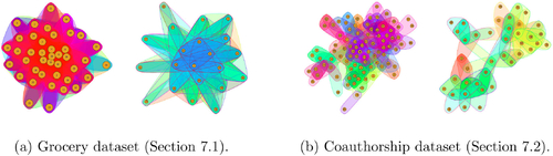
Fig. 1 Examples of hypergraph datasets. (b) shows co-tagging data and (c) shows a subsample of the coauthorship network of Ji and Jin (2016). The figures were made with R packages HyperG (Marchette 2021) and igraph (Csardi and Nepusz 2006).

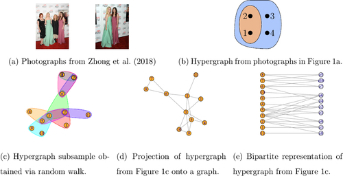
More formally, a hypergraph $G=(V,E)$ consists of a set of N node labels V and M hyperedges E, where $e\in E$ contains no repeated elements and $e\subseteq V$ (see Figure 1(c)). This data type can also be equivalently represented as a bipartite graph with an $(N\times M)$ adjacency tensor in which each hyperedge is indexed by a node and an edge from a population node to a hyperedge node indicates presence in a hyperedge (see Figure 1(e)). Although a significant portion of the existing literature relies on the bipartite representation, we focus on the former representation since it allows us to develop a model which allows for an arbitrary number of hyperedges by avoiding conditioning on M.

We consider extending the latent distance model of Hoff, Raftery, and Handcock (2002) to the hypergraph setting using the representation in Figure 1(c). In this approach, a low-dimensional coordinate is associated with each node and nodes whose latent coordinates are close in terms of Euclidean distance are assumed more likely to share a tie. This modeling choice is appealing since the latent space offers an intuitive visualization of the data, encourages transitive relationships due to the metric property of Euclidean distance and allows control over the joint distribution of subgraph counts. Models of this type also allow quantification of uncertainty in interaction probabilities and prediction of future interactions. In our model, we wish to harness hypergraph analogues of these properties and we focus on the following inferential questions.

• (Q1)How can we determine an intuitive visualization of an observed hypergraph?

• (Q2)How do we expect new nodes to interact with the observed hypergraph relationships?

There is a growing literature concerned with hypergraph modeling (Battiston et al. 2020), and several graph models have been extended to the bipartite setting. Examples include exponential random graphs (Wang, Pattison, and Robins 2013), blockmodels (Doreian, Batagelj, and Ferligoj 2004) and latent space network models (Friel et al. 2016). However, in contrast to our work, models for bipartite representations assume the number of hyperedges is known and fixed.

Examples of models for general hypergraphs include the β model of Stasi et al. (2014), preferential attachment models (Wang et al. 2010) and the clustering-based model of Ng and Murphy (2021). In a m-uniform hypergraph all hyperedges contain exactly m elements, and extensions of stochastic blockmodels (see Ghoshdastidar and Dukkipati 2017; Chien, Lin, and Wang 2018) and graphons (Balasubramanian 2021) have been studied for this hypergraph type. Simplicial hypergraphs, or rather simplicial complexes (see Edelsbrunner and Harer 2010), are a significant class of hypergraphs in which the presence of a hyperedge implies the presence of all subsets of that hyperedge. Proposed models for simplicial complexes include an analogue of exponential random graphs (Zuev, Eisenberg, and Krioukov 2015), preferential attachment based models (Bianconi and Rahmede 2017), simplicial configuration models (Young et al. 2017) and the recursive models of Kahle (2014). A discussion of random simplicial complexes is presented in Kahle (2014) and work on geometric simplicial complexes (Bobrowski and Kahle 2018) is most related to our proposed procedure. Simplicial complexes also appear more broadly in the statistics literature (Chazal and Michel 2017; Lunagómez et al. 2017) and our terminology “simplicial hypergraph” is nonstandard.

Our focus on inference for the full generality of hypergraphs marks a distinction between our work and much of the existing literature. By considering general hypergraphs, we avoid restrictions inherent to simplicial and uniform representations and this allows us to consider how hyperedges of different orders interact in the data. Non-simplicial hypergraph arise in many settings and particular instances of non-simplicial coauthorship networks are presented in Figure 1(d) and Section 7.2.

The main contributions of this article are as follows. First, using the representation shown in Figure 1(c), we develop a computationally tractable latent space model for non-simplicial hypergraph data. Second, we explore the novel application of Bookstein coordinates to address non-identifiability in the latent representation. Third, we perform inference on hypergraph data that is outside the reach of competing methods and consider a novel application of delayed acceptance MCMC methodology. Finally, we study properties of the degree distribution for our model and present approximate theoretical results.

The rest of this article is organized as follows. Section 2 provides the background for the hypergraph model presented in Section 3. Section 4 considers the degree distribution of our model and Section 5 describes a procedure for obtaining posterior samples. The simulation studies and real data examples are presented in Sections 6 and 7, respectively, and we conclude with a discussion in Section 8.

2 Background

2.1 Latent Space Network Modeling

Latent space models were introduced for network data in Hoff, Raftery, and Handcock (2002). This modeling framework associates the nodes of a network with low-dimensional latent coordinates and expresses the probability of edges forming as a function of the latent representation.

To describe this model for a N node network, we let $\mathit{Y}={\left\{y_{ij}\right\}}_{i,j=1,2,\dots ,N}$ denote the observed $(N\times N)$ adjacency matrix, where y_ij represents the connection between nodes i and j. For binary interactions, we take y_ij = 1 if i and j share an edge and y_ij = 0 otherwise. We also let $u_i\in {\mathbb{R}}^d$ denote the d-dimensional latent coordinate associated with the ith node, for $i=\{1,2,\dots ,N\}=[N]$. The presence of an edge is then given by (1) $$\begin{array}{cc}{Y}_{ij}\hfill & \sim \text{Bernoulli}(p_{ij}),\hspace{1em}{p}_{ij}=P(y_{ij}=1|u_i,u_j,\theta )\hfill \\ \hfill & =1/\left(1+\hspace{0.17em}\exp \hspace{0.17em}\{-f(u_i,u_j,\theta )\}\right),\hfill \end{array}$$(1) for $i,j\in [N]$, where θ represents additional model parameters and f controls how u_i and u_j affect the propensity for ties to form. Typically, f is specified as monotonically decreasing in a measure of similarity between u_i and u_j . For example, Hoff, Raftery, and Handcock (2002) take (2) $$f(u_i,u_j,\theta )=\alpha -\Vert u_i-u_j\Vert ,$$(2) where $\Vert ·\Vert$ is the Euclidean distance, and $\theta =(\alpha )$ represents the base-rate tendency for edges to form. The function f may also be adapted to incorporate covariate information so that nodes which share certain characteristics are more likely to be connected. The likelihood, conditional on $\mathit{U}={\left\{u_i\right\}}_{i=1}^N$ and θ, is given by (3) $$\begin{array}{c}\mathcal{L}(\mathit{U},\theta ;\mathit{Y})\propto \prod _{i<j}P{(y_{ij}=1|u_i,u_j,\theta )}^{y_{ij}}\\ \hspace{1em}\times {\left[1-P(y_{ij}=1|u_i,u_j,\theta )\right]}^{1-y_{ij}}.\end{array}$$(3)

Properties of this model are well-understood and we refer to Rastelli, Friel, and Raftery (2016) for details.

2.2 Random Geometric Graphs

Random geometric graphs (RGGs) (Penrose 2003) can be viewed as a special case of the latent space network model outlined in Section 2.1. To express the connection probabilities we let $B_r(u_i)=\{u\in {\mathbb{R}}^d|\Vert u-u_i\Vert \le r\}$, where $\Vert ·\Vert$ is Euclidean distance, denote a ball of radius r with center u_i . The presence of an edge is then expressed deterministically as (4) $$\begin{array}{c}{p}_{ij}=P(y_{ij}=1|u_i,u_j,r)=\mathbb{1}\left(B_r(u_i)\cap B_r(u_j)\ne \varnothing \right)\\ =\mathbb{1}\left(\Vert u_i-u_j\Vert \le 2r\right),\end{array}$$(4) so that nodes i and j share a tie only if their corresponding sets have a nonempty intersection (see Figure 2) or, equivalently, when $\Vert u_i-u_j\Vert \le 2r$.

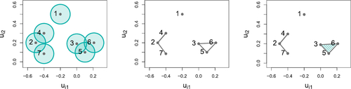
Fig. 2 Example of a Čech complex. Left: $B_r(u_i)$ for ${\{u_i=(u_{i1},u_{i2})\}}_{i=1}^7$ in ${\mathbb{R}}^2$. Middle: the graph obtained by taking pairwise intersections. Right: the hypergraph obtained by taking intersections of arbitrary order. The shaded region indicates an order 3 hyperedge.

We can now express the likelihood of observing Y conditional on U and r as (5) $$\begin{array}{c}\mathcal{L}(\mathit{U},r;\mathit{Y})\propto \prod _{i<j}\mathbb{1}{(\Vert u_i-u_j\Vert \le 2r)}^{y_{ij}}\\ \hspace{1em}\times {\left[1-\mathbb{1}(\Vert u_i-u_j\Vert \le 2r)\right]}^{1-y_{ij}}.\end{array}$$(5)

Since a RGG is deterministic conditional on U and r, (5) is equal to 1 only when there is a perfect correspondence between the observed connections Y and the connections induced by the latent positions and radius, and is otherwise equal to 0.

2.3 Random Geometric Hypergraphs

We can extend the RGG from Section 2.2 to hypergraphs by considering the full intersection pattern of convex sets. To begin, we introduce the concept of a nerve (Edelsbrunner and Harer 2010, sec. 3.2) in the following definition.

Definition 2.1.

(Nerve) Let $\mathcal{A}={\left\{A_i\right\}}_{i=1}^N$ represent a collection of non-empty sets. The nerve of $\mathcal{A}$ is given by $\mathit{Nrv}(\mathcal{A})=\left\{\sigma \subseteq \{1,2,\dots ,N\}|\underset{j\in \sigma }{\cap }{A}_j\ne \varnothing \right\}$.

The nerve represents the sets of indices whose corresponding regions have a non-empty intersection. The sets $\left\{1\right\},\left\{2\right\},\dots ,\left\{N\right\}$ are included in $\mathit{Nrv}(\mathcal{A})$ and $\left|\sigma \right|\le N$ for $\sigma \in \mathit{Nrv}(\mathcal{A})$, where $\left|\sigma \right|$ is the order of the set. The nerve defines a hypergraph where $\sigma \in \mathit{Nrv}(\mathcal{A})$ represents a hyperedge, and for sets ${\sigma }_1\in \mathit{Nrv}(\mathcal{A})$ and ${\sigma }_2\subset {\sigma }_1$, it follows immediately that ${\sigma }_2\in \mathit{Nrv}(\mathcal{A})$ implying that the hypergraph is simplicial (Kahle 2017).

Taking $A_i=B_r(u_i)$, as for the RGG in Section 2.2, gives rise to the well-studied Čech complex (Edelsbrunner and Harer 2010, sec. 3.2). This is defined below.

Definition 2.2

(Čech Complex). For a set of coordinates $\mathit{U}={\left\{u_i\right\}}_{i=1}^N$ and a radius r, the Čech complex ${\mathcal{C}}_r(\mathit{U})$ is given by ${\mathcal{C}}_r(\mathit{U})=\mathit{Nrv}({\{B_r(u_i)\}}_{i=1}^N)$.

We now introduce a subset of the Čech complex known as the k-skeleton.

Definition 2.3

(k-skeleton of the Čech Complex). Let ${\mathcal{C}}_r(\mathit{U})$ denote the Čech complex, as given in Definition 2.2. The k-skeleton of ${\mathcal{C}}_r(\mathit{U})$ is given by ${\mathcal{C}}_r^{(k)}(\mathit{U})=\{\sigma \in {\mathcal{C}}_r(\mathit{U})$ $\left|\right|\sigma |\le k\}$.

Example 2.1.

For the Čech complex in Figure 2, ${\mathcal{C}}_r(\mathit{U})=\left\{\right\{1\},\{2\},\{3\},\{4\},\{5\},\{6\},\{7\},\{2,4\}$, {2, 7}, {3, 5}, {3, 6}, {5, 6}, $\{3,5,6\}\},{\mathcal{C}}_r^{(1)}(\mathit{U})=\{\left\{1\right\},\left\{2\right\},\left\{3\right\},\left\{4\right\},\left\{5\right\},\left\{6\right\},\left\{7\right\}\}$, ${\mathcal{C}}_r^{(2)}(\mathit{U})={\mathcal{C}}_r^{(1)}\cup \left\{\right\{2,4\},\{2,7\},$ $\{3,5\},\{3,6\},\{5,6\}\}$, and ${\mathcal{C}}_r^{(3)}(\mathit{U})={\mathcal{C}}_r^{(2)}(\mathit{U})\cup \{3,5,6\}$.

3 Latent Space Hypergraphs

3.1 Motivation and Notation

In the motivating examples from Section 1, we observed arbitrary hypergraph interactions. Since the models discussed in Section 2 express either pairwise or simplicial interactions, they are not appropriate for this data. This motivates the development of a non-simplicial latent space hypergraph model. We aim to propose a model which has (i) a convenient and computationally tractable likelihood with (ii) a support that is simple to describe.

We consider general hypergraphs on N nodes and let K denote the maximum hyperedge order, where $2\le K\le N$. Let ${\mathcal{G}}_{N,K}=({\mathcal{V}}_N,{\mathcal{E}}_{N,K})$ denote the space of hypergraphs on N and K, where ${\mathcal{V}}_N=\{1,2,\dots ,N\}$ and ${\mathcal{E}}_{N,K}$ represent the node labels and hyperedges up to order K on N nodes, respectively. Additionally, let ${\mathcal{E}}_N^k$ represent hyperedges of exactly order k on N nodes, so that ${\mathcal{E}}_{N,K}={\cup }_{k=2}^K{\mathcal{E}}_N^k$, and let $e_k\in {\mathcal{E}}_N^k$ denote an order k interaction, where $\left|e_k\right|=k$ and e_k contains no repeated elements.

3.2 Combining k-skeletons

To extend the model in Section 2.3 to express non-simplicial hypergraphs we allow the radii to differ for each hyperedge order. We generate a hypergraph by isolating the order k hyperedges from the complex ${\mathcal{C}}_{r_k}(\mathit{U})$ and combining these for $k=2,3,\dots ,K$, where $r_k\ne r_{k\prime }$ for $k\ne k\prime$. For example, when K = 3, we take radii r₂ and r₃ along with their Čech complexes ${\mathcal{C}}_{r_2}(\mathit{U})$ and ${\mathcal{C}}_{r_3}(\mathit{U})$. Then, we consider the order 2 hyperedges in ${\mathcal{C}}_{r_2}(\mathit{U})$ and the order 3 hyperedges in ${\mathcal{C}}_{r_3}(\mathit{U})$, as shown in Figure 3. We refer to a hypergraph constructed in this way as a non-simplicial random geometric hypergraph (nsRGH).

Fig. 3 Example of a nsRGH (see Definition 3.1) with $\mathit{U}={\left\{u_i\right\}}_{i=1}^7={\{(u_{i1},u_{i2})\}}_{i=1}^7$. Left: ${\mathcal{C}}_{r_2}(\mathit{U})$. Middle: ${\mathcal{C}}_{r_3}(\mathit{U})$. Right: ${\cup }_{k=2}^3{\mathcal{D}}_{r_k}^{(k)}(\mathit{U})$.

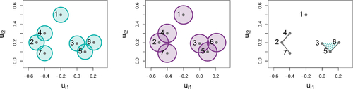
Definition 3.1

(nsRGH). Take $\mathit{r}=(r_2,r_3,\dots ,r_K)$ such that $r_k>r_{k-1}>0$ for $k=3,4,\dots ,K$. We define a nsRGH on N nodes as the hypergraph $g_{N,K}(\mathit{U},\mathit{r})$ with hyperedges given by ${\cup }_{k=2}^K{\mathcal{D}}_{r_k}^{(k)}(\mathit{U})$, where ${\mathcal{D}}_{r_k}^{(k)}(\mathit{U})={\mathcal{C}}_{r_k}^{(k)}(\mathit{U})\setminus {\mathcal{C}}_{r_k}^{(k-1)}(\mathit{U})$ denotes the hyperedges of exactly order k in the Čech complex with radius r_k and ${\mathcal{C}}_{r_k}^{(k)}(\mathit{U})$ is as in Definition 2.3.

Example 3.1.

For the nsRGH shown in the right panel of Figure 3 we have $g_{7,3}(\mathit{U},\mathit{r})={\mathcal{D}}_{r_2}^{(2)}(\mathit{U})\cup {\mathcal{D}}_{r_3}^{(3)}(\mathit{U})$, where ${\mathcal{D}}_{r_2}^{(2)}(\mathit{U})=\left\{\right\{2,4\},\{2,7\},\{3,5\},\{5,6\left\}\right\}$, and ${\mathcal{D}}_{r_3}^{(3)}(\mathit{U})=\{3,5,6\}$.

In Definition 3.1 constraints are imposed on the radii $\mathit{r}=(r_2,r_3,\dots ,r_K)$ to ensure that the hypergraphs are non-simplicial since for example, if $r_3<r_2$ and the hyperedge {i, j, k} is present in the hypergraph, it follows that $\{i,j\},\{i,k\}$, and {j, k} must also be present.

3.3 Generative Model and Likelihood

Our procedure for generating a nsRGH $g_{N,K}(\mathit{U},\mathit{r})$ (see Definition 3.1) is deterministic conditional on U and r. Practical application of this model is therefore challenging since (i) the probability observing a hypergraph $h_{N,K}\in {\mathcal{G}}_{N,K}$ is binary (similarly to the RGG in Section 2.2) and (ii) it is difficult to characterize the space of hypergraphs which can be expressed as a nsRGH. These issues hinder estimation via likelihood methods and make it difficult to say whether a latent representation can be found a priori.

To address these issues we consider a modification of the nsRGH $g_{N,K}(\mathit{U},\mathit{r})$, denoted $g_{N,K}^{*}(\mathit{U},\mathit{r},\mathbf{\phi })$, obtained by independently modifying the state of each order k hyperedge in $g_{N,K}(\mathit{U},\mathit{r})$ with probability ${\phi }_k\in [0,1]$. More precisely, if $y_{e_k}^{(g)}\in \{0,1\}$ is the state of e_k in $g_{N,K}^{*}(\mathit{U},\mathit{r},\mathbf{\phi })$ where $y_{e_k}^{(g)}=1$ indicates presence, we take $y_{e_k}^{(g^{*})}=(y_{e_k}^{(g)}+s_k)\hspace{1em}\mathrm{mod}2$, where $y_{e_k}^{(g^{*})}\in \{0,1\}$ is the state of hyperedge e_k in $g_{N,K}^{*}(\mathit{U},\mathit{r},\mathbf{\phi })$ and $S_k\sim \text{Bernoulli}({\phi }_k)$. This means that $y_{e_k}^{(g)}$ is modified from either present to absent or absent to present with probability ${\phi }_k$ to obtain $y_{e_k}^{(g^{*})}$. The noise terms ${\left\{{\phi }_k\right\}}_{k=2}^K$ control the amount of modification of $g_{N,K}(\mathit{U},\mathit{r})$, and so setting ${\phi }_k$ close to 0 obtains a hypergraph that is similar to a nsRGH.

To fully specify a generative model, we assign a probability distribution on the latent coordinates U. We let $u_i\stackrel{\text{iid}}{\sim }\mathcal{N}(\mu ,\Sigma )$, for $i\in [N]$ to reflect the intuition that nodes placed more centrally in the latent representation are likely to have high degrees and neighbors with high degrees. A hypergraph can now be generated by the procedure given in Algorithm 1, and details of efficient implementation of this are given in supplements C and E.3.

Algorithm 1

Sample a hypergraph $g_{N,K}^{*}$ given $N,K,\mathit{r},\mathbf{\phi },\mu$, and Σ.

Sample $\mathit{U}={\left\{u_i\right\}}_{i=1}^N$ such that $u_i\stackrel{\text{iid}}{\sim }\mathcal{N}(\mu ,\Sigma )$, for $i=1,2,\dots ,N$.

For $k=2,3,\dots ,K$,

a) Given U and r_k , check which $e_k=\{i_1,i_2,\dots ,i_k\}\in {\mathcal{E}}_N^k$ satisfy $y_{e_k}^{(g)}=1$.

To determine if $y_{e_k}^{(g)}=1$, check that ${\cap }_{l=1}^k{B}_{r_k}(u_{i_l})\ne \varnothing$.

b) For all $e_k\in {\mathcal{E}}_N^k$, sample $S_k\sim \text{Bernoulli}({\phi }_k)$.

Let $y_{e_k}^{(g^{*})}=(y_{e_k}^{(g)}+s_k)\hspace{1em}\mathrm{mod}2$

To express the likelihood of observing the hypergraph $h_{N,K}\in {\mathcal{G}}_{N,K}$, we let (6) $$d_k(g_{N,K}(\mathit{U},\mathit{r}),h_{N,K})=\sum _{e_k\in {\mathcal{E}}_N^k}|y_{e_k}^{(g)}-y_{e_k}^{(h)}|$$(6) denote the discrepancy between the order k hyperedges in $g_{N,K}(\mathit{U},\mathit{r})$ and $h_{N,K}$, where $k=2,3,\dots ,K$ and $y_{e_k}^{(h)}\in \{0,1\}$ indicates the state of e_k in $h_{N,K}$. Intuitively, the distance (6) corresponds to the number of hyperedges whose state differs between $h_{N,K}$ and $g_{N,K}(\mathit{U},\mathit{r})$. We note that evaluating this distance does not require the ${\sum }_{k=2}^K(\begin{array}{c}N\\ k\end{array})$ computations suggested by (6), and refer to the supplement for details.

Given this notion of hypergraph distance the likelihood of observing $h_{N,K}$, conditional on $\mathit{U},\mathit{r}$, and $\mathbf{\phi }$, can be written as (7) $$\begin{array}{c}\mathcal{L}(\mathit{U},\mathit{r},\mathbf{\phi };h_{N,K})\propto \prod _{k=2}^K{\phi }_k^{d_k(g_{N,K}(\mathit{U},\mathit{r}),h_{N,K})}\\ \mathrm{\hspace{1em}}\mathrm{\hspace{1em}}\times {(1-{\phi }_k)}^{\left(\begin{array}{c}N\\ k\end{array}\right)-d_k(g_{N,K}(\mathit{U},\mathit{r}),h_{N,K})}.\end{array}$$(7)

This follows by considering which hyperedges in $g_{N,K}(\mathit{U},\mathit{r})$ must have their state modified to match the hyperedges in $h_{N,K}$, and which hyperedges are the same as in $h_{N,K}$. Since our likelihood is of the same form as (Lunagómez, Olhede, and Wolfe 2020, proof of Proposition 3.1), it follows that hypergraphs with a greater number of hyperedge modification are less likely for $0<{\phi }_k<1/2$ and so (7) behaves in an intuitive way.

The model specification is complete with the following priors for $k=2,3,\dots ,K$ (8) $$\begin{array}{c}\mu \sim \mathcal{N}(m_{\mu },{\Sigma }_{\mu })\hspace{1em}{\Sigma }_{\mu }\sim {\mathcal{W}}^{-1}(\Phi ,\nu ),\hspace{1em}{r}_k\sim \hspace{0.17em}\exp \hspace{0.17em}({\lambda }_k),\hspace{1em}\text{and}\\ {\phi }_k\sim \mathrm{B}(a_k,b_k),\end{array}$$(8) where ${\mathcal{W}}^{-1}(·,·)$ and $B(·,·)$ denote an Inverse-Wishart and Beta, respectively.

3.4 Can We Improve Model Flexibility?

In a nsRGH, the constraint $r_k>r_{k-1}$, for $k=3,\dots ,K$, ensures that the interactions are non-simplicial. However, this implies r_k will impact the higher-order hyperedges and, to improve model flexibility, we introduce additional modification parameters. In Algorithm 1 the noise ${\phi }_k$ is applied independently across all hyperedges of order k and, alternatively, we can modify each hyperedge depending on its state in $g_{N,K}(\mathit{U},\mathit{r})$. For $k=2,3,\dots ,K$, let ${\mathit{\psi }}^0=({\psi }_2^0,{\psi }_3^0,\dots ,{\psi }_K^0)\in [0,1]$ denote the probability of modifying the state of a hyperedge in $g_{N,K}(\mathit{U},\mathit{r})$ from absent to present, and let ${\mathit{\psi }}^1=({\psi }_2^1,{\psi }_3^1,\dots ,{\psi }_K^1)\in [0,1]$ denote the probability of modifying the state of a hyperedge in $g_{N,K}(\mathit{U},\mathit{r})$ from present to absent. Crucially, for large k, the term ${\psi }_k^1$ may increase to account for the discrepancy between the density of order k hyperedges in $h_{N,K}$ and $g_{N,K}(\mathit{U},\mathit{r})$. This generative model is summarized in Algorithm A.1 in the supplement and, as commented in Section 3.3, we can implement this without the suggested ${\sum }_{k=2}^K(\begin{array}{c}N\\ k\end{array})$ likelihood computations. Further details of this are given in the supplement, as highlighted in Section 3.3.

As in Section 3.3, the likelihood of observing $h_{N,K}$ is based on a distance metric, (9) $$d_k^{(ab)}(g_{N,K}(\mathit{U},\mathit{r}),h_{N,K})=\#\{e_k\in {\mathcal{E}}_N^k|y_{e_k}^{(g)}=a\cap y_{e_k}^{(h)}=b\},$$(9) which records the number of hyperedges that have state $a\in \{0,1\}$ in $g_{N,K}(\mathit{U},\mathit{r})$ and state $b\in \{0,1\}$ in $h_{N,K}$. For example, $d_k^{(01)}(g_{N,K}(\mathit{U},\mathit{r}),h_{N,K})$ represents the number of hyperedges absent in $g_{N,K}(\mathit{U},\mathit{r})$ and present in $h_{N,K}$. Efficient evaluation of (9) is discussed in supplement E.3.2 and the likelihood conditional on $\mathit{U},\mathit{r},{\mathit{\psi }}^1$, and ${\mathit{\psi }}^0$ is given by (10) $$\begin{array}{c}\mathcal{L}\left(\mathit{U},\mathit{r},{\mathit{\psi }}^1,{\mathit{\psi }}^0;h_{N,K}\right)\propto \prod _{k=2}^K[{\left({\psi }_k^1\right)}^{d_k^{(10)}(g_{N,K}(\mathit{U},\mathit{r}),h_{N,K})}\\ \hspace{1em}\times {\left(1-{\psi }_k^1\right)}^{d_k^{(11)}(g_{N,K}(\mathit{U},\mathit{r}),h_{N,K})}\\ \hspace{1em}\times {\left({\psi }_k^0\right)}^{d_k^{(01)}(g_{N,K}(\mathit{U},\mathit{r}),h_{N,K})}\\ \hspace{1em}\times {\left(1-{\psi }_k^0\right)}^{d_k^{(00)}(g_{N,K}(\mathit{U},\mathit{r}),h_{N,K})}]\mathrm{}.\end{array}$$(10)

We obtain (10) in a similar way to (7), and note that (10) is equivalent to (7) when ${\psi }_k^1={\psi }_k^0={\phi }_k$, for $k=2,3,\dots ,K$.

The model specification is complete with the following priors for $k=2,3,\dots ,K$ (11) $$\begin{array}{c}\mu \sim \mathcal{N}(m_{\mu },{\Sigma }_{\mu }),\hspace{1em}{\Sigma }_{\mu }\sim {\mathcal{W}}^{-1}(\Phi ,\nu ),\hspace{1em}{r}_k\sim \hspace{0.17em}\exp \hspace{0.17em}({\lambda }_k),\\ {\psi }_k^0\sim \mathrm{B}\left(a_k^0,b_k^0\right),\hspace{1em}{\psi }_k^1\sim \mathrm{B}\left(a_k^1,b_k^1\right),\end{array}$$(11) where ${\mathcal{W}}^{-1}(·,·)$ and $B(·,·)$ denote an Inverse-Wishart and Beta, respectively.

3.5 Identifiability

For the model presented in Section 3.3, the joint distribution of the hypergraph $g_{N,K}^{*}(\mathit{U},\mathit{r},\mathbf{\phi })$ and its associated nsRGH (see Definition 3.1) $g_{N,K}(\mathit{U},\mathit{r})$ can be decomposed as follows. (12) $$\begin{array}{c}p(g_{N,K}^{*}(\mathit{U},\mathit{r},\mathbf{\phi }),g_{N,K}(\mathit{U},\mathit{r})|\mu ,\Sigma ,\mathbf{\phi },\mathit{r})=\\ p\left(g_{N,K}^{*}(\mathit{U},\mathit{r},\mathbf{\phi })|g_{N,K}(\mathit{U},\mathit{r}),\mathbf{\phi }\right)p\left(g_{N,K}(\mathit{U},\mathit{r})|\mu ,\Sigma ,\mathit{r}\right)\mathrm{}.\end{array}$$(12)

Note that a similar decomposition exists for the model given in Section 3.4.

The hyperedges expressed by the conditional distribution $p(g_{N,K}(\mathit{U},\mathit{r})|\mu ,\Sigma ,\mathit{r})$ are determined through the positions of their relative latent coordinates and are therefore unchanged given distance-preserving transformations of U and scaling of U and r. We address this non-identifiability by defining U on the Bookstein space of coordinates (see Bookstein 1986; Dryden and Mardia 1998, sec. 2.3.3 and details in Supplement B) which determine a translation, rotation and rescaling of U with respect to a set of anchor points. These anchor points are fixed throughout the posterior sampling procedure (see Section 5) and also address the non-identifiability associated with rescaling r.

Removing non-identifiability in U is typically achieved via Procrustes analysis (Dryden and Mardia 1998) in which a post-processing step is included to remove the effect of distance-preserving transformations of U (Hoff, Raftery, and Handcock 2002). This approach can be used for our model, providing that scaling between U and r is accounted for. By using Bookstein coordinates, we instead work directly with our posterior samples on a quotient space (Dryden and Mardia 1998) which accounts for distance-preserving transformations. This approach avoids the additional computation associated with the Procrustes transformation.

Finally, a hyperedge in our model can be expressed by either the geometric or noise component. To maintain the properties imposed by $g_{N,K}(\mathit{U},\mathit{r})$, we wish to keep the noise $\mathbf{\phi }$ small. When there are few observed hyperedges, it will become increasingly difficult to distinguish between these competing sources. This implies an additional source of non-identifiability which we address by ensuring the noise terms $\mathbf{\phi }$ are sufficiently small via prior distributions.

4 Theoretical Results

We now study the behavior of the node degree in the hypergraph model detailed in Algorithm 1. Since the nodes in our hypergraph model are exchangeable, it is sufficient to study the degree properties of the ith node, and it is straightforward to extend the results in this section to the model detailed in Algorithm A.1.

To begin, we make explicit the following properties of our hypergraph model: (P1) A hypergraph generated from our model is a modification of a nsRGH (see Definition 3.1), and (P2) Conditional on U and r, hyperedges of each order occur independently in our model. We also make the following assumptions: (A1) The number of nodes N and maximum hyperedge order K are fixed, and (A2) The covariance of the latent coordinates Σ is diagonal, where ${\Sigma }_{ll}={\sigma }_{ll}^2$ for $l=1,2,$ $\dots ,d$. Note that (A2) is not restrictive since we can obtain this by applying a distance-preserving transformation to our point cloud in ${\mathbb{R}}^d$.

Following Section 3, we denote a hypergraph obtained by modifying the nsRGH $g_{N,K}(\mathit{U},\mathit{r})$ as $g_{N,K}^{*}(\mathit{U},\mathit{r},\mathbf{\phi })$, and we let $y_{e_k}^{(g)}$ and $y_{e_k}^{(g^{*})}$ indicate the presence or absence of the hyperedge e_k in $g_{N,K}(\mathit{U},\mathit{r})$ and $g_{N,K}^{*}(\mathit{U},\mathit{r},\mathbf{\phi })$, respectively. The degree of node i in a hypergraph is given by the number of hyperedges which contain i and, for node i in $g_{N,K}(\mathit{U},\mathit{r})$, we denote the order k degree as ${\mathrm{Deg}}_{(i,k)}^{(g)}=\sum _{\{e_k\in {\mathcal{E}}_N^k|i\in e_k\}}{y}_{e_k}^{(g)}$ and the full degree as ${\mathrm{Deg}}_{(i)}^{(g)}={\sum }_{k=2}^K{\mathrm{Deg}}_{(i,k)}$. Analogous expressions for $g_{N,K}^{*}(\mathit{U},\mathit{r},\mathbf{\phi })$ are obtained by replacing g with $g^{*}$. To organize our results, we separate the discussion into hyperedges with order k = 2 and $k\ge 3$. Proofs can be found in Supplement F.

4.1 Degree Properties for k = 2

We begin by restating a result from Rastelli, Friel, and Raftery (2016) which allows us to express the degree distribution and average degree for order k = 2 hyperedges in our model. Throughout, we write hyperedges of order 2 that contain node i as {i, j}.

Theorem 4.1

(Reproduced from (Rastelli, Friel, and Raftery 2016, Theorem 1)). Let $p_{\{i,j\}}(u_i|\theta )$ denote the probability of node i with latent coordinate u_i belonging to an order 2 hyperedge in the model detailed in Section 3.3, conditional on $\theta =(r_2,{\phi }_2,\mu ,\Sigma )$. The degree distribution of order 2 hyperedges for the ith node for our hypergraph model, conditional on θ, is given by (13) $$\begin{array}{c}p\left({\mathrm{Deg}}_{i,2}^{(g^{*})}=l|\theta \right)=\int p(u_i|\mu ,\Sigma )\left(\begin{array}{c}N-1\\ l\end{array}\right)p_{\{i,j\}}\\ \hspace{1em}{(u_i|\theta )}^l{(1-p_{\{i,j\}}(u_i|\theta ))}^{N-1-l} d{u}_i,\end{array}$$(13) where ${\mathrm{Deg}}_{(i,2)}^{(g)}=\sum _{\{e_2\in {\mathcal{E}}_{N,2}|i\in e_2\}}{y}_{e_2}^{(g)}$, and the average degree is given by (14) $${\overline{d}}_2^{(g^{*})}(\theta )=(N-1)\int p(u_i|\mu ,\Sigma )p_{\{i,j\}}(u_i|\theta ) d{u}_i.$$(14)

Proof.

See Supplement F. □

In order to apply this result, we must derive an expression for $p_{\{i,j\}}(u_i|\theta )$. This is given in the following proposition.

Proposition 4.1

(Probability of an order k = 2 hyperedge). Let $e_2=\{i,j\}$ denote an order k = 2 hyperedge. The probability of e₂ occurring in $g^{*}$, given that node i has latent position u_i , can be expressed as (15) $$\begin{array}{c}{p}_{\{i,j\}}\left(y_{ij}^{(g^{*})}=1|{\theta }_1\right)=p\left(y_{\{i,j\}}^{(g)}=1|{\theta }_2\right)(1-{\phi }_2)\\ +\left(1-p\left(y_{\{i,j\}}^{(g)}=1|{\theta }_2\right)\right){\phi }_2,\end{array}$$(15) where ${\theta }_1=(u_i,r_2,{\phi }_2,\mu ,\Sigma ),{\theta }_2=(u_i,r_2,\mu ,\Sigma )$ and $p(y_{\{i,j\}}^{(g)}=1|{\theta }_2)$ denotes the probability of $e_2=\{i,j\}$ being present in $g_{N,K}(\mathit{U},\mathit{r})$ when node i is positioned at u_i . It follows that $p(y_{\{i,j\}}^{(g)}=1|{\theta }_2)=p({(U_j^{*})}^T{U}_j^{*}\le 4r_2^2)$, where $U_j^{*}=U_j-u_i\sim \mathcal{N}(\mu -u_i,\Sigma )$. Then (16) $${(U_j^{*})}^T{U}_j^{*}\sim \sum _{l=1}^d{\sigma }_l^2{\chi }_{1,{({(\mu -u_i)}_l/{\sigma }_l)}^2}^2,$$(16) where ${(\mu -u_i)}_l$ is the lth component of $(\mu -u_i)$, for $l=1,2,\dots ,d$ and $\Sigma =\text{diag}({\sigma }_1^2,{\sigma }_2^2,\dots ,{\sigma }_d^2)$.

Proof.

See Supplement F. □

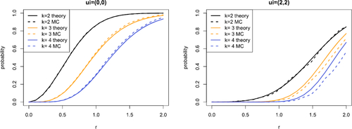
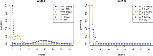
Theorem 4.1 and Proposition 4.1 allow us to evaluate properties of the node degree of order k = 2 hyperedges, where the intractable integrals (13) and (14) are evaluated using numerical methods. It is straightforward to calculate (16) when the variances are constant, but for general diagonal Σ, we require numerical evaluation as implemented in the R package CompQuadForm (Duchesne and de Micheaux 2010). The expression for the connection probabilities in Proposition 4.1 is validated for an example in Figure 4.

Fig. 4 Comparison of theoretical (solid) and Monte Carlo (dashed) estimates of $p(y_{e_{k,i}}^{(g)}=1|u_i,r_k,\mu ,\Sigma )$ for varying r_k . We take $\Sigma =\text{diag}(1,1),\mu =(0,0)$ and consider connection probabilities for k = 2, 3, 4. In the left plot $u_i=\mu$ and in the right plot $u_i=(1,2)$. The same study with $\Sigma =\text{diag}(1,2)$ is provided in Supplement F.3.

4.2 Degree Properties for $k\ge 3$

We now present some results for the order k degree distribution. First, note that the expression for the degree distribution of order k = 2 hyperedges, given in Theorem 4.1, arises since hyperedges {i, j} occur independently given u_i . This is no longer true for higher-order hyperedges since, for example, if k = 3 it is clear that hyperedges {i, j, l} and {i, j, m} are not independent given i. Deriving an exact expression for the order k degree distribution is therefore challenging, and we consider an approximation of this in the following proposition where we denote an order k hyperedge containing node i as $e_{k,i}$.

Proposition 4.2

(Approximate order k degree distribution). Let $p_{e_{k,i}}(y_{e_{k,i}}^{(g^{*})}=1|{\theta }_k)$ denote the probability of node i with latent position u_i belonging to an order k hyperedge, denoted as $e_{k,i}$, in the model detailed in Section 3.3, conditional on ${\theta }_k=(u_i,r_k,{\phi }_k,\mu ,\Sigma )$. Conditional on $r_k,{\phi }_k,\mu$, and Σ, the degree distribution of order $k\ge 3$ hyperedges for the ith node for our hypergraph model is approximately (17) $$\begin{array}{c}p\left({\mathrm{Deg}}_{i,k}^{(g^{*})}=l|\theta \right)\\ \mathrm{\hspace{1em}}\mathrm{\hspace{1em}}\approx \int p(u_i|\mu ,\Sigma )\frac{{\left(\lambda (N,k,{\theta }_k)\right)}^l\hspace{0.17em}\exp \hspace{0.17em}\left(-\lambda (N,k,{\theta }_k)\right)}{l!} d{u}_i\end{array}$$(17) where $\lambda (N,k,{\theta }_k)=(\begin{array}{c}N-1\\ k-1\end{array})p(y_{e_{k,i}}^{(g^{*})}=1|{\theta }_k)$ and ${\mathrm{Deg}}_{(i,k)}^{(g^{*})}=\sum _{\{e_k\in {\mathcal{E}}_N^k|i\in e_k\}}{y}_{e_k}^{(g^{*})}$.

Proof.

See Supplement F. □

This proposition relies on a Poisson approximation to the sum of dependent Bernoulli trials. Bounds for the quality of this approximation have been studied (e.g., see Teerapabolarn 2014), and it is well-understood that this approximation will degrade as either the number of possible hyperedges, as controlled by N and k, or the connection probability $p_{e_{k,i}}(u_i|r_k,{\phi }_k,\mu ,\Sigma )$ grows, or both.

As in the previous section, we require an expression for $p_{e_{k,i}}(u_i|r_k,{\phi }_k,\mu ,\Sigma )$ to explore this distribution. As in Proposition 4.1, an order k hyperedge can be expressed either by the geometric or noise component of our model, where the probability of occurrence in $g_{N,K}(\mathit{U},\mathit{r})$ is the more challenging to determine. Recall that this quantity is given by the probability that the balls of radius r_k corresponding to the nodes in $e_{k,i}$ have a non-empty intersection, so that the hyperedge $e_{k,i}=\{i,i_2,i_3,\dots ,i_k\}$ is present in $g_{N,K}(\mathit{U},\mathit{r})$ if ${\cap }_{j\in e_{k,i}}{B}_{r_k}(u_j)\ne \varnothing$. This condition is equivalent to the coordinates ${\left\{u_j\right\}}_{j\in e_{k,i}}$ lying within a ball of radius r_k (see Supplement E.3.1). Since the latent coordinates are assumed to follow a Normal distribution, evaluating this probability requires the evaluation of an intractable integral (see Gilliland 1962). To address this we consider an approximation of this quantity in which the region of integration is approximated by a square of side length s_k , denoted as $S_{s_k}$. We choose $s_k=\sqrt{\pi }{r}_k$ so that it has an equal area to a disk of radius r_k . This choice simplifies the region of integration by allowing each dimension to be considered independently. Alternative choices for the distribution on the latent coordinates, such as the uniform, may be more amenable to analytic expressions for the degree distribution and we leave exploration of this to future work.

Lemma 4.1

(Probability of an order $k\ge 3$ hyperedges). We can express the probability of an order k hyperedge containing node i, denoted as $e_{k,i}$, being present in $g^{*}$ conditional on the latent coordinate u_i as (18) $$\begin{array}{c}p\left(y_{e_{k,i}}^{(g^{*})}=1|{\theta }_{1,k}\right)=p\left(y_{e_{k,i}}^{(g)}=1|{\theta }_{2,k}\right)(1-{\phi }_k)\\ \mathrm{\hspace{1em}}\mathrm{\hspace{1em}}+\left(1-p\left(y_{e_{k,i}}^{(g)}=1|{\theta }_{2,k}\right)\right){\phi }_k,\end{array}$$(18) where ${\theta }_{1,k}=(u_i,r_k,{\phi }_k,\mu ,\Sigma ),{\theta }_{2,k}=(u_i,r_k,\mu ,\Sigma )$ and $p(y_{e_{k,i}}^{(g)}=1|{\theta }_{2,k})$ is the probability of the order k hyperedge $e_{k,i}=\{i,i_2,i_3,$ $\dots ,i_k\}$ being present in $g_{N,K}(\mathit{U},\mathit{r})$ given u_i .

The probability of $e_{k,i}$ occurring in $g_{N,K}(\mathit{U},\mathit{r})$ with $U_j\sim \mathcal{N}(\mu ,\Sigma )$, conditional on u_i , can then be approximated as follows. (19) $$\begin{array}{c}p\left(y_{e_{k,i}}^{(g)}=1|{\theta }_{2,k}\right)\approx \prod _{l=1}^d[(k-1)\int f(u|{\mu }_l,{\sigma }_l)\\ \hspace{1em}\times {\left[F(u+\sqrt{\pi }{r}_k|{\mu }_l,{\sigma }_l)-F(u|{\mu }_l,{\sigma }_l)\right]}^{k-2}\\ \hspace{1em}\times \mathbb{1}(u_i\in (u,u+\sqrt{\pi }{r}_k)) du\\ \hspace{1em}+{\left[F(u_i+\sqrt{\pi }{r}_k|{\mu }_l,{\sigma }_l)-F(u_i|{\mu }_l,{\sigma }_l)\right]}^{k-1}\mathrm{}]\mathrm{},\end{array}$$(19) where $f(·|{\mu }_l,{\sigma }_l)$ and $F(·|{\mu }_l,{\sigma }_l)$ denote the pdf and cdf of the random variable with distribution $\mathcal{N}({\mu }_l,{\sigma }_l^2)$, μ_l denotes the lth element of μ and $\Sigma =\text{diag}({\sigma }_1^2,{\sigma }_2^2,\dots ,{\sigma }_d^2)$.

Proof.

See Supplement F. □

These results allow us to examine the behavior of the degree distribution. We consider the quality of the $p(y_{e_{k,i}}^{(g)}=1|u_i,r_k,\mu ,\Sigma )$ approximation and the Poisson approximation in Figures 4 and 5, respectively. Since hyperedges in our model may come from the latent coordinates and or the random noise, similar connection probabilities can occur through different parameter combinations. However, we should find such combinations have notable differences in the degree distribution and other properties such as, for instance, motif counts and measures of transitivity. The above calculations suggest that examining such properties theoretically is likely to be challenging. Techniques such as those used in Kahle (2017) may be applied here, however, our choice of underlying distribution on the latent coordinates is likely to limit their applicability.

Fig. 5 Comparison between empirical (dashed line) and Poisson approximation (points) of the order k = 3 degree distribution conditional on the latent coordinate u_i . We take $N=10,\mu =(0,0),\Sigma =\text{diag}(1,1)$ and evaluate the distribution for $r_3\in (0.1,0.4,1.0)$. The left plot shows $u_i=\mu$ and the right plot shows $u_i=(1,2)$. The equivalent Figures with $\Sigma =\text{diag}(1,2)$ and N = 20 are given in Supplement F.3.

5 Posterior Sampling

Here we outline our posterior sampling scheme for the model detailed in Section 3.3 and note that this can be modified to sample from the model in Section 3.4. Posterior samples are obtained via a Metropolis-Hastings-within-Gibbs MCMC scheme (Gamerman and Lopes 2006, sec. 6.4.2) with a delayed acceptance (DA) update (Banterle et al. 2019) for the latent positions and algorithmic details of our MCMC scheme are given in Supplement E.

First, recall that we define U on the Bookstein space of coordinates (Section 3.5) so that a set of anchor points remain fixed throughout estimation. For $u_i\in {\mathbb{R}}^d$, let the d anchor points be denoted by $\{u_{B_1},u_{B_2},\dots ,u_{B_d}\}$. Then, for $i\in \{1,2,\dots ,N\}\backslash \{B_1,B_2,\dots ,B_d\}$ we propose ${\mathit{U}}^{*}$ with ith entry $u_i^{*}=u_i+{ϵ}_u$ where ${ϵ}_u\sim \mathcal{N}(0,{\sigma }_u{I}_d)$ and $u_j^{*}=u_j$ for $j\ne i$. This proposal is then accepted as a sample from $p(\mathit{U}|\mu ,\Sigma ,\mathit{r},{\mathit{\psi }}^0,{\mathit{\psi }}^1,h_{N,K})$ with probability (20) $$A{R}_{u_i}=\min \left\{1,\frac{\mathcal{L}({\mathit{U}}^{*},\mathit{r},{\mathit{\psi }}^1,{\mathit{\psi }}^0;h_{N,K})p(u_i^{*}|\mu ,\Sigma )}{\mathcal{L}(\mathit{U},\mathit{r},{\mathit{\psi }}^1,{\mathit{\psi }}^0;h_{N,K})p(u_i|\mu ,\Sigma )}\right\}\mathrm{}.$$(20)

Calculating the hypergraph $g_{N,K}(\mathit{U},\mathit{r})$ presents a computational bottleneck in evaluating the likelihood (20). We utilize the GUDHI library (The GUDHI Project 2021) to perform this calculation and find that the cost of calculating the order k hyperedges in $g_{N,K}(\mathit{U},\mathit{r})$ grows with both N and k. This suggests our target is a natural candidate for delayed acceptance in which terms of the likelihood are sequentially included in order of increasing computational cost, allowing for a faster and computationally cheaper rejection of poor proposals. Let $h_N^k$ denote the observed hyperedges of order k and write (21) $$\begin{array}{c}A{R}_{u_i}=\min \{1,\underset{{\rho }_2(\mathit{U},{\mathit{U}}^{*})}{\underbrace{\frac{p(h_{N,2}|{\mathit{U}}^{*},r_2,{\psi }_2^1,{\psi }_2^0)p(u_i^{*}|\mu ,\Sigma )}{p(h_{N,2}|\mathit{U},r_2,{\psi }_2^1,{\psi }_2^0)p(u_i|\mu ,\Sigma )}}}\\ \times \underset{{\rho }_k(\mathit{U},{\mathit{U}}^{*})}{\underbrace{\prod _{k=3}^K\frac{p(h_N^k|{\mathit{U}}^{*},r_k,{\psi }_k^1,{\psi }_k^0)}{p(h_N^k|\mathit{U},r_k,{\psi }_k^1,{\psi }_k^0)}}}\}\mathrm{},\end{array}$$(21) where $p(h_N^k|\mathit{U},r_k,{\psi }_k^1,{\psi }_k^0)$ denotes the contribution of the order k hyperedge terms in (10), for $k=2,3,\dots ,K$. Following Banterle et al. (2019), we take ${\rho }_k(\mathit{U},{\mathit{U}}^{*})$ as specified in (21) and accept ${\mathit{U}}^{*}$ if each intermediary rate $\min \{1,{\rho }_k(\mathit{U},{\mathit{U}}^{*})\}$ indicates acceptance as outlined in Algorithm E.1 in the supplement.

The kth radii is updated according to a standard random-walk MH step, where the proposal $r_k^{*}=r_k+{ϵ}_r$ with ${ϵ}_r\sim \mathcal{N}(0,{\sigma }_r)$, is accepted with probability (22) $$\min \left\{1,\frac{p(h_N^k|\mathit{U},r_k^{*},{\phi }_k)p(r_k^{*}|{\lambda }_k)}{p(h_N^k|\mathit{U},r_k,{\phi }_k)p(r_k|{\lambda }_k)}\right\}\mathrm{}.$$(22)

The remaining parameters can be sampled directly from their full conditionals and updated via a Gibbs step. Full details are presented in the supplement and we note here that our implementation also incorporates adaptive updates for U and r as detailed in Vihola (2012) and implemented in the R library ramcmc (Helske 2021).

6 Simulations

Sections 6.1 evaluate the efficacy of our approach by investigating predictive distributions, and Section 6.2 explores the scalability of our sampling procedure. Additional simulation studies on model-depth and misspecification are presented in supplements H and K.

6.1 Assessing Model Fit

For this study, we simulate a hypergraph from the model outlined in Algorithm 1 with $N=50,d=2,K=3,\mathit{r}=(0.35,0.45),{\mathbf{\phi }}_0={\mathbf{\phi }}_1=(0.001,0.001),\mu =(0,0)$ and $\Sigma =(\begin{array}{cc}1& 0\\ 0& 1\end{array})$ and examine the performance of our MCMC scheme through inspection of the predictive degree distribution. After 5000 post burn-in iterations we obtain posterior mean estimates to (2 significant figures) $\widehat{\mathit{U}}$, $\widehat{\mathit{r}}=(0.11,0.15),{\widehat{\mathit{\psi }}}^0={\widehat{\mathit{\psi }}}^1=(0.00108,0.00011),\widehat{\mu }=(0.081,0.12)$ and $\widehat{\Sigma }=(\begin{array}{cc}0.082& 0.015\\ 0.015& 0.091\end{array})$. Since the anchor coordinates specify a scaling on the estimated latent positions, we cannot make a direct comparison between the true and estimated model parameters (see supplementary Figures I.8 and I.9).

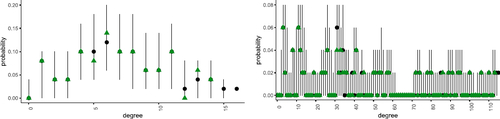
We can instead examine the posterior predictive distribution and compare this to the simulated hypergraph. If the sampling procedure has produced meaningful estimates, we expect a reasonable correspondence between these two quantities. Since a hypergraph is a complex object, we make a comparison by summarising each hypergraph by its degree distribution. Figure 6 shows this separately for the degree distributions of order k = 2 and k = 3 hyperedges. Overall we see that there is reasonable overlap between these distributions. For completeness, we also summarize the output of the MCMC scheme in Supplement I where we see that the sampling procedure appears to have converged and the estimated latent coordinates correspond reasonably to the truth.

Fig. 6 Comparison of true and posterior predictive degree distributions for hyperedges of order k = 2 (left) and k = 3 (right). Vertical lines and black dots correspond to the range and median of the probabilities of observing each degree as calculated via the posterior predictive. The observed degree is shown as green triangles.

6.2 Scalability Study

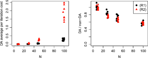
Our MCMC scheme (see Section 5) updates the latent coordinates via a delayed acceptance (DA) step that allows poor proposals to be quickly rejected on a subset of the likelihood. Here we substantiate our claim that this offers computational advantages over a standard Metropolis-Hastings update on data simulated according to Algorithm 1 by comparing average per-iteration cost times for an MCMC scheme implemented with and without DA. Since the computational cost is closely connected to the number of nodes N and the density of the hypergraphs, we consider timings for hypergraphs with increasing N under two different density regimes, referred to as (R1) and (R2). We specify the parameters for each regime so that (R1) generates sparser hypergraphs than (R2). Details of the specific parameters are given in Supplement J alongside plots of the density of the simulated data.

This study allows us to examine the scalability of our approach as N grows and to demonstrate the reduction in computational cost offered by DA. Figure 7 reports average per-iteration times for the DA MCMC scheme for both regimes in addition to the ratio of average per-iteration times for a DA and non-DA MCMC scheme. This figure confirms our intuitions that hypergraphs with a larger N are more computationally challenging, and this cost increases as the density of the hypergraphs grows. By inspecting the right-hand plot of Figure 7, we observe that incorporating DA into our MCMC offers a significant improvement in average per-iteration cost. We note that this relative improvement increases with N and is largely unaffected by the density of the hypergraphs. Whilst K remains fixed throughout this section, we do expect the improvements offered by DA to increase with K.

Fig. 7 Summary of average per-iteration costs after 200 iterations for an MCMC implemented with and without delayed acceptance (DA) for 10 datasets sampled from data regimes (R1) (black, circle) and (R2) (red, triangle). Left: average per-iteration cost in seconds for a DA scheme. Right: ratio of average per-iteration cost for a DA scheme and a scheme without DA. Numbers less than 1 imply DA offers a computational speed-up.

7 Real Data Examples

In this section we analyze two hypergraph datasets using the model from Algorithm A.1 of the supplement. These examples describe grocery co-purchases and academic coauthorship (Figure 8).

Fig. 8 Visualization of the datasets considered in Section 7. The hyperedges correspond to the observations for each dataset. Each figure shows the full hypergraph (left) and a subset sampled according to a random walk (right).

7.1 Grocery Items

Here we consider a subset of the grocery transaction data available as part of the R package arules (Hahsler et al. 2007). Here, each node corresponds to a category of items and each hyperedge indicates whether a set of items were bought together. To analyze this data we take a random subset of size N = 41 with K = 6 and hold back $N^{*}=4$ nodes for validation of the predictive distribution for additional nodes. Since the hyperedges can be expressed through the geometric or noise component of our model, we impose constraints on the noise terms to ensure that the set of hyperedges explained by the latent positions is non-empty. More specifically, we limit the order k noise terms so that they cannot exceed 90% of the density of the order k hyperedges in the observed hypergraph. With these constraints, we implemented our MCMC scheme for 100,000 iterations and discarded the first three quarters as burn-in. Figure L.14 in the supplement depicts the observed hypergraph with the nodes positioned at posterior mean of the latent coordinates $\widehat{\mathit{U}}$ and we obtain the posterior mean estimate of the radii $\widehat{\mathit{r}}=(1.096,1.097,1.101,1.107,1.11)$. Traceplots for each parameter are shown in Supplement L and the average per-iteration cost was 0.012 min.

To select the $N^{*}$ nodes for which we evaluate the predictive distribution, we take the nodes with the smallest eigen-centralities in the graph obtained by connecting all node pairs who share a hyperedge. 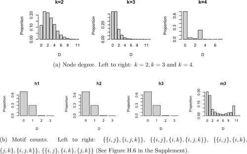To reflect how these nodes were selected, we then sample additional latent coordinates from the posterior predictive by first obtaining $N+N^{*}$ samples from $\mathcal{N}({\mu }^{(i)},{\Sigma }^{(i)})$ and then selecting the $N^{*}$ coordinates that are furthest from the mode ${\mu }^{(i)}$ in terms of Euclidean distance. Similarly to Section 6.1, we summarize the predictive hypergraphs by considering node degree and motif counts and Figure 9 reports the results of this. In particular, for each measure, we report the proportion of predictive samples which have discrepancy D from the true observed value where D denotes the absolute difference between the prediction and the truth. Overall, we see that the majority of samples have either zero or close to zero discrepancy from the observed values, suggesting that we reasonably capture the unobserved interaction patterns. We believe that the uptick in the upper tail for some of the motif counts does not have a structural explanation and is simply an artifact of this particular data example. Note that we do not observe this behavior for the coauthorship dataset presented in Section 7.2.

Fig. 9 Summary of predictive distributions for $N^{*}$ additional nodes for the Grocery dataset. For each measure we report the proportion of predictions which are distance D from the truth, where D is the absolute difference between the predictive and the truth.

7.2 Coauthorship for Statisticians

We now repeat the analysis from the previous section for a hypergraph with larger N. In this section we consider a coauthorship hypergraph constructed from the DBLP dataset,¹ presented in Mao, Sarkar, and Chakrabarti (2020) and available online.² From this dataset we construct a subset of size N = 99 with K = 4 via a random walk and, similarly to Section 7.1, we hold out $N^{*}=10$ of these nodes according to the graph eigen-centrality and use these to validate predictive inference. We fit the model outlined in Section 3.4 by implementing our MCMC for 400,000 iterations and taking the initial 3/4th of these as burn-in. Given equivalent restrictions on the noise parameters as described for the previous example, we obtain the posterior mean of the radii $\widehat{\mathit{r}}=(0.23,0.25,0.31)$ and the posterior means of the latent position as shown in Figure L.14 in the supplement. The average per-iteration cost for our scheme was 0.012 min and traceplots showing convergence for the model parameters are given in supplement L. 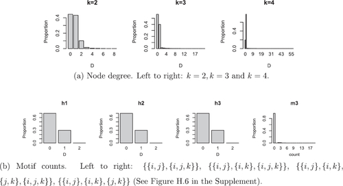A summary of the predictive distribution of the $N^{*}$ additional nodes is given in Figure 10 and, for all summaries of the predicted interactions, we find that the majority of the discrepancies between the predicted and true values are zero or close to zero. This suggests the predicted interaction patterns are close to the truth.

Fig. 10 Summary of predictive distributions for $N^{*}$ additional nodes for the coauthorship dataset. For each measure we report the proportion of predictions which are distance D from the truth, where D is the absolute difference between the predictive and the truth.

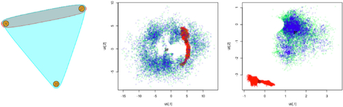
To provide further justification for our assumption of increasing radii we compare our model to a restricted version with a simplicial geometric component in which r_k = r for $k=2,3,\dots ,K$. Since this data example is non-simplicial, we expect that the latent representation in the restricted model will be less informative for the hyperedges than the latent representation for our model. To verify this, we present the latent coordinate traceplots for a subset of the data in Figure 11 for both models. By comparing the middle and right panels of this figure, we see that the latent coordinates are more constrained for our model with a non-simplicial geometric component. This behavior occurs because the restricted model expresses the observed interactions by deleting hyperedges from a simplicial motif whilst our model aims to express the non-simplicial motif directly through the geometric component. Since a simplicial motif occurs when all latent positions are sufficiently close, this means that the traceplot does not allow us to distinguish between the latent positions in the restricted model. Contrast this with our model in which the node labeled “22” is distinctly separated from the nodes labeled “27” and “31”.

Fig. 11 Comparison between latent positions for subset of the coauthorship network on nodes {22, 27, 31}. Left: observed interactions. Middle: traceplot of latent positions for model with r_k = r. Right: traceplot of latent positions for our model with $r_k>r_{k-1}$.

8 Discussion

Our proposed model allows hyperedges to be expressed by a geometric or noise component, and we keep the noise term small to impose desirable properties on the hypergraphs. The geometric component of our model may be unable to express certain hypergraph relationships and this is made clear by considering, for example, that the maximum number of leaves in a star is limited by the latent space dimension. This may be mediated by choosing an alternative geometric simplicial complex to generate the nerve, increasing the probability of hyperedge modification, or taking a different specification for the latent positions.

There exist several modeling extensions which could be considered for our framework, such as modeling nonbinary hyperedges, the addition of community structure analogously to Handcock, Raftery, and Tantrum (2007), or the introduction of covariate information. Additional avenues for future work follow from considering other choices for the nerve construction, latent geometry and restrictions on the radii. For example, we could instead use the more scalable Vietoris-Rips complex (Edelsbrunner and Harer 2010), consider non-Euclidean embeddings (Krioukov et al. 2010) or explore models with node-specific radii. However, it is important to stress that estimation for a given modification of our model may be challenging. Even for our proposed model, scalability remains a key limitation and this may be exacerbated by certain extensions. While we found that delayed acceptance offered computational improvements, it remains an open line of enquiry to consider how methodology to improve scalability for latent space networks (Raftery et al. 2012; Salter-Townshend and Murphy 2013) may be adapted to this setting.

Acknowledgments

Thank you to Tin Lok James Ng for providing the Star Wars dataset analyzed in a previous version of this work and Matthew Kahle, Sandipan Roy, Brendan Murphy and Marco Battiston for helpful comments. We acknowledge the High End Computing facility at Lancaster University and are grateful to Daniel Grose for creating the associated R package.

Supplementary Materials

The supplementary materials contain additional details on Bookstein coordinates.

Disclosure Statement

No potential conflict of interest was reported by the author(s).

Additional information

Funding

We acknowledge the support of the EPSRC funded EP/L015692/1 STOR-i CDT and EPSRC grants EP/S00159X/1, EP/R01860X/1 and EP/V022636/1. This work was supported, in part, by NSF awards CAREER IIS-1149662 and IIS-1409177, by ONR awards YIP N00014-14-1-0485 and N00014-17-1-2131.

Notes

1 https://dblp.uni-trier.de/xml/

2 https://xueyumao.github.io/coauthorship

References

- Balasubramanian, K. (2021), “Nonparametric Modeling of Higher-Order Interactions via Hypergraphons,” Journal of Machine Learning Research, 22, 1–35.
- Banterle, M., Grazian, C., Lee, A., and Robert, C. P. (2019), “Accelerating Metropolis-Hastings Algorithms by Delayed Acceptance,” Foundations of Data Science, 1, 103–128. DOI: 10.3934/fods.2019005.
- Battiston, F., Cencetti, G., Iacopini, I., Latora, V., Lucas, M., Patania, A., Young, J.-G., and Petri, G. (2020), “Networks Beyond Pairwise Interactions: Structure and Dynamics,” Physics Reports, 874, 1–92. DOI: 10.1016/j.physrep.2020.05.004.
- Bianconi, G., and Rahmede, C. (2017), “Emergent Hyperbolic Network Geometry,” Scientific Reports, 7, 41974. DOI: 10.1038/srep41974.
- Bobrowski, O., and Kahle, M. (2018), “Topology of Random Geometric Complexes: A Survey,” Journal of Applied and Computational Topology, 1, 331–364. DOI: 10.1007/s41468-017-0010-0.
- Bookstein, F. L. (1986), “Size and Shape Spaces for Landmark Data in Two Dimensions,” Statistical Science, 1, 181–222. DOI: 10.1214/ss/1177013696.
- Chazal, F., and Michel, B. (2017), “An Introduction to Topological Data Analysis: Fundamental and Practical Aspects for Data Scientists,” Frontiers in Artificial Intelligence, 4, 667963. DOI: 10.3389/frai.2021.667963.
- Chien, I., Lin, C.-Y., and Wang, I.-H. (2018), “Community Detection in Hypergraphs: Optimal Statistical Limit and Efficient Algorithms,” in International Conference on Artificial Intelligence and Statistics (Vol. 84), pp. 871–879, PMLR.
- Csardi, G., and Nepusz, T. (2006), “The igraph Software Package for Complex Network Research,” InterJournal, complex systems, 1695.5, 1–9.
- Doreian, P., Batagelj, V., and Ferligoj, A. (2004), “Generalized Blockmodeling of Two-Mode Network Data,” Social Networks, 26, 29–53. DOI: 10.1016/j.socnet.2004.01.002.
- Dryden, I. L., and Mardia, K. V. (1998), Statistical Shape Analysis, Chichester: Wiley.
- Duchesne, P., and de Micheaux, P. L. (2010), “Computing the Distribution of Quadratic Forms: Further Comparisons between the Liu-Tang-Zhang Approximation and Exact Methods,” Computational Statistics and Data Analysis, 54, 858–862. DOI: 10.1016/j.csda.2009.11.025.
- Edelsbrunner, H., and Harer, J. (2010), Computational Topology - an Introduction, Providence, RI: American Mathematical Society.
- Friel, N., Rastelli, R., Wyse, J., and Raftery, A. E. (2016), “Interlocking Directorates in Irish Companies Using a Latent Space Model for Bipartite Networks,” Proceedings of the National Academy of Sciences, 113, 6629–6634. DOI: 10.1073/pnas.1606295113.
- Gamerman, D., and Lopes, H. F. (2006), Markov Chain Monte Carlo: Stochastic Simulation for Bayesian Inference (2nd ed.), London: Chapman and Hall/CRC.
- Ghoshdastidar, D., and Dukkipati, A. (2017), “Consistency of Spectral Hypergraph Partitioning Under Planted Partition Model,” The Annals of Statistics, 45, 289–315. DOI: 10.1214/16-AOS1453.
- Gilliland, D. C. (1962), “Integral of the Bivariate Normal Distribution over an Offset Circle,” Journal of the American Statistical Association, 57, 758–768. DOI: 10.1080/01621459.1962.10500813.
- Hahsler, C. B., Buchta, C., Gruen, B., Hornik, K., Borgelt, C., Johnson, I., and Ledmi, M. (2021), arules: Mining Association Rules and Frequent Itemsets, R package version 1.6-8.
- Handcock, M. S., Raftery, A. E., and Tantrum, J. M. (2007), “Model-based Clustering for Social Networks,” Journal of the Royal Statistical Society, Series A, 170, 301–354. DOI: 10.1111/j.1467-985X.2007.00471.x.
- Helske, J. (2021), ramcmc: Robust Adaptive Metropolis Algorithm, R package version 0.1.1.
- Hoff, P. D., Raftery, A. E., and Handcock, M. S. (2002), “Latent Space Approaches to Social Network Analysis,” Journal of the American Statistical Association, 97, 1090–1098. DOI: 10.1198/016214502388618906.
- Ji, P., and Jin, J. (2016), “Coauthorship and Citation Networks for Statisticians,” The Annals of Applied Statistics, 10, 1779–1812. DOI: 10.1214/15-AOAS896.
- Kahle, M. (2017), “Random Simplicial Complexes,” in Handbook of Discrete and Computational Geometry, eds. J. E. Goodman, J. O’Rourke, and C. D. Tóth, pp. 581–604, Boca Raton, FL: CRC Press.
- Kahle, M. (2014), “Topology of Random Simplicial Complexes: A Survey,” AMS Contemporary Mathematics, 620, 201–222.
- Kolaczyk, E. D. (2009), Statistical Analysis of Network Data: Methods and Models (1st ed.), New York: Springer.
- Krioukov, D., Papadopoulos, F., Kitsak, M., Vahdat, A., and Boguñá, M. (2010), “Hyperbolic Geometry of Complex Networks,” Physical Review E, 82, 036106. DOI: 10.1103/PhysRevE.82.036106.
- Lunagómez, S., Mukherjee, S., Wolpert, R. L., and Airoldi, E. M. (2017), “Geometric Representations of Random Hypergraphs,” Journal of the American Statistical Association, 112, 363–383. DOI: 10.1080/01621459.2016.1141686.
- Lunagómez, S., Olhede, S. C., and Wolfe, P. J. (2020), “Modeling Network Populations via Graph Distances,” Journal of the American Statistical Association, 116, 2023–2040. DOI: 10.1080/01621459.2020.1763803.
- Mao, X., Sarkar, P., and Chakrabarti, D. (2020), “Estimating Mixed Memberships with Sharp Eigenvector Deviations,” Journal of the American Statistical Association, 116, 1928–1940. DOI: 10.1080/01621459.2020.1751645.
- Marchette. (2021), HyperG: Hypergraphs in R, R package version 1.0.0.
- Ng, T. L. J., and Murphy, T. B. (2021), “Model-based Clustering for Random Hypergraphs,” Advances in Data Analysis and Classification, 16, 691–723. DOI: 10.1007/s11634-021-00454-7.
- Penrose, M. (2003), Random Geometric Graphs. Oxford Studies in Probability. Oxford: Oxford University Press.
- Raftery, A. E., Niu, X., Hoff, P. D., and Yeung, K. Y. (2012), “Fast Inference for the Latent Space Network Model Using a Case-Control Approximate Likelihood,” Journal of Computational and Graphical Statistics, 21, 901–919. DOI: 10.1080/10618600.2012.679240.
- Rastelli, R., Friel, N., and Raftery, A. E. (2016), “Properties of Latent Variable Network Models,” Network Science, 4, 407–432. DOI: 10.1017/nws.2016.23.
- Salter-Townshend, M., and Murphy, T. B. (2013), “Variational Bayesian Inference for the Latent Position Cluster Model for Network Data,” Computational Statistics & Data Analysis, 57, 661–671. DOI: 10.1016/j.csda.2012.08.004.
- Stasi, D., Sadeghi, K., Rinaldo, A., Petrović, S., and Fienberg, S. E. (2014), “β Models for Random Hypergraphs with a Given Degree Sequence,” ArXiv e-prints.
- Teerapabolarn, K. (2014), “An Improvement of Poisson Approximation for Sums of Dependent Bernoulli Random Variables,” Communications in Statistics - Theory and Methods, 43, 1758–1777. DOI: 10.1080/03610926.2012.674606.
- The GUDHI Project (2021), GUDHI User and Reference Manual. GUDHI Editorial Board, 3.4.1 edition.
- Vihola, M. (2012), “Robust Adaptive Metropolis Algorithm with Coerced Acceptance Rate,” Statistics and Computing, 22, 997–1008. DOI: 10.1007/s11222-011-9269-5.
- Wang, J.-W., Rong, L.-L., Deng, Q.-H., and Zhang, J.-Y. (2010), “Evolving Hypernetwork Model,” The European Physical Journal B, 77, 493–498. DOI: 10.1140/epjb/e2010-00297-8.
- Wang, P., Pattison, P., and Robins, G. (2013), “Exponential Random Graph Model Specifications for Bipartite Networks—A Dependence Hierarchy,” Social Networks, 35, 211–222. DOI: 10.1016/j.socnet.2011.12.004.
- Young, J.-G., Petri, G., Vaccarino, F., and Patania, A. (2017), “Construction of and Efficient Sampling from the Simplicial Configuration Model,” Physical Review E, 96, 032312. DOI: 10.1103/PhysRevE.96.032312.
- Zhong, Y., Arandjelovic, R., and Zisserman, A. (2018), “Compact Deep Aggregation for Set Retrieval,” in Proceedings of the European Conference on Computer Vision Workshops.
- Zuev, K., Eisenberg, O., and Krioukov, D. (2015), “Exponential Random Simplicial Complexes,” Journal of Physics A: Mathematical and Theoretical, 48, 465002. DOI: 10.1088/1751-8113/48/46/465002.