Bayesian Spline-Based Hidden Markov Models with Applications to Actimetry Data and Sleep Analysis

Abstract

B-spline-based hidden Markov models employ B-splines to specify the emission distributions, offering a more flexible modeling approach to data than conventional parametric HMMs. We introduce a Bayesian framework for inference, enabling the simultaneous estimation of all unknown model parameters including the number of states. A parsimonious knot configuration of the B-splines is identified by the use of a trans-dimensional Markov chain sampling algorithm, while model selection regarding the number of states can be performed based on the marginal likelihood within a parallel sampling framework. Using extensive simulation studies, we demonstrate the superiority of our methodology over alternative approaches as well as its robustness and scalability. We illustrate the explorative use of our methods for data on activity in animals, that is whitetip-sharks. The flexibility of our Bayesian approach also facilitates the incorporation of more realistic assumptions and we demonstrate this by developing a novel hierarchical conditional HMM to analyse human activity for circadian and sleep modeling. Supplementary materials for this article are available online.

KEYWORDS:

• Accelerometer data
• Bayesian hidden Markov models
• Bayesian splines
• Circadian and sleep modeling
• Model selection
• Reversible-jump MCMC

1 Introduction

The class of hidden Markov models (HMMs) offers a powerful approach for extracting information from sequential data (Rabiner 1989). A basic N-state HMM consists of a discrete-time stochastic process $(x_t,y_t)$ where x_t is an unobserved N-state time-homogeneous Markov chain, and $y_t|x_t\sim f_{x_t}(y_t)$ with the emission distributions $f_{x_t}$ belonging to some parametric family such as normal or gamma. However, a parametric HMM is often too restrictive for complex real data (Zucchini, MacDonald, and Langrock 2016). It is recognized that simple parametric choices for the emission distributions are not always justified, and moreover, their misspecification can lead to seriously erroneous inference on the number and classification of hidden states (Yau et al. 2011; Pohle et al. 2017). Semi- and nonparametric modeling of emission distributions offer more flexibility and/or may serve as exploratory tools to investigate the suitability of a parametric family; see Piccardi and Pérez (2007) for activity recognition in videos, Yau et al. (2011) for the analysis of genomic copy number variation, Langrock et al. (2015, 2018) for modeling animal movement data and Kang et al. (2019) for delineating the pathology of Alzheimer’s disease, among many others. Theoretical guarantees for inference in such models have been studied in a number of recent papers. Notably Alexandrovich, Holzmann, and Leister (2016) proved that model parameters and the order of the Markov chain are identifiable (up to permutations of the hidden states labels) if the transition probability matrix of $\left\{x_t\right\}$ has full rank and is ergodic, and if the emission distributions are distinct. These conditions are fairly generic and in practice will usually be satisfied. We also refer to Gassiat, Cleynen, and Robin (2016a), Gassiat and Rousseau (2016b) for further identifiability results, and to Vernet (2015), De Castro, Gassiat, and Le Corff (2017), and references therein, for further theoretical results on inference under nonparametric settings. The increased flexibility and modeling accuracy obtained by nonparametric emission distributions comes at a higher computational cost. For instance, the cost of the standard HMM algorithms (e.g., the forward-backward algorithm of Rabiner 1989) for kernel-based HMMs (Piccardi and Pérez 2007) is subject to a quadratic growth with data size n and thus can be prohibitive for long time series data. Bayesian nonparametric HMMs (Yau et al. 2011) built on Dirichlet process mixture models pose challenges to the existing sampling methods due to the increased complexity of the model space (Hastie, Liverani, and Richardson 2015).

Splines have good approximation properties for a rich class of functions (De Boor et al. 1978; Schumaker 2007). A spline function of order O is a piecewise polynomial function of degree O – 1 where the polynomial pieces are connected at the so-called knot points. Provided these are distinct, the derivatives of piecewise polynomials are (O – 2)-times continuously differentiable at the knots. B-splines (short for basis splines) of order O provide basis functions for representing spline functions of the same order defined over the same set of knots (De Boor et al. 1978). The great flexibility and nice computational properties of the B-splines make them a popular tool in semi-/nonparametric statistical modeling, especially in nonlinear regression analysis (Denison et al. 2002; Zanini et al. 2020) and density estimation (Koo 1996; Edwards, Meyer, and Christensen 2019). Incorporating B-splines into HMMs is attractive for real applications as two powerful aspects can be exploited, the forward-backward algorithm for efficient HMM inference, and the flexibility for estimating the emission densities. A frequentist estimation approach for HMM based on penalized B-splines (P-splines) was introduced by Langrock et al. (2015, 2018). It requires pre-specifying the number and positions of knots where, in practice, a large number of knots are needed to ensure flexibility, leading to computational challenges (e.g., convergence to suboptimal local extreme of the likelihood) and cost. Also to date the selection of the state-specific smoothing parameters and the quantification of parameter uncertainty remain challenging inferential tasks in the frequentist framework. Current methods rely on cross-validation and parametric bootstrap techniques (Langrock et al. 2015), which are extremely computationally intensive and can be numerically unstable especially for increasing cardinality N. Hence, their approach is so far only feasible for models with a small N which may severely limit its applicability.

As far as we are aware spline-based methods have not yet been considered for emission density estimation in a Bayesian formulation of HMMs. The aim of this article is to propose and develop a methodology that achieves exactly this by means of an almost “tuning-free” reversible jump Markov chain Monte Carlo (RJMCMC) algorithm (Green 1995), which exploits (i) the forward filtering backward sampling (FFBS) procedure for efficient simulation of the hidden state process, (ii) a stochastic approximation based adaptive MCMC scheme for automatic tuning, (iii) a reparameterization scheme for enhancing the sampling efficiency and (iv) an adaptive knot selection scheme that modifies and extends ideas considered in other scenarios such as DiMatteo, Genovese, and Kass (2001) and Sharef et al. (2010) for flexible emission modeling. We report results demonstrating significant advantages of our proposed adaptive spline based algorithm. Compared to current alternative spline-based approaches, namely the frequentist P-spline approach of Langrock et al. (2015), and a Bayesian adaptive P-spline (Lang and Brezger 2004) approach which is newly adapted here for density estimation in HMMs, our method generally achieves higher estimation accuracy and efficiency while maintaining a much lower model complexity. It also performs favorably over the Gaussian mixture based HMM in more challenging data-generating scenarios.

Estimating N is often a question of scientific interest in itself and introduces an additional level of complexity to HMM inference. While order estimation has been extensively studied for parametric HMMs, such as in Celeux and Durand (2008), Pohle et al. (2017), and Frühwirth-Schnatter and Frèuhwirth-Schnatter (2006), few theoretical or practical results have been obtained for the semi- or nonparametric case, which often requires the number of states to be known or fixed in advance (Piccardi and Pérez 2007; Yau et al. 2011; Lehéricy 2018). Recently, Lehéricy (2019) proposed two estimators for N, which are theoretically attractive but suffer from implementation difficulties such as non-convex optimization problems and heuristic tuning. In this article, we address this issue with a fully Bayesian approach to the selection of N through a parallel sampling scheme that is both easy to implement and computationally efficient. Quantities such as the marginal likelihood for each model can be easily estimated.

Among the numerous application fields of HMMs, there is a growing interest within the context of e-Health to gain insight into an individual’s health status based on relevant biomarker data. Physical activity (PA) is receiving much attention as an important biomarker of the sleep-wake cycle and circadian timing system, which is closely associated with our physical and mental health (Roenneberg and Merrow 2016). PA can be easily and objectively measured in a non-obtrusive way under normal living conditions using accelerometry or actigraphy through wearable sensing devices. Huang et al. (2018) investigated PA using a HMM with circadian-clock driven transition probabilities and, amongst various circadian parameters of interest, they proposed a novel model-derived circadian parameter for monitoring and quantifying a subject’s circadian rhythm. An advantage of a further Bayesian formulation is that the modularity of its components can be used to perform inference rigorously even in a more complex hierarchical HMM model. As a further contribution based on our proposed Ansatz, we develop a hierarchical conditional HMM that may be applied to (i) characterize the sleep-wake patterns in the overall PA data of an individual and (ii) analyze sleep patterns of an individual in a refined way through a “sub-HMM” that is conditional on the “rest” state inferred from (i).

The article is structured as follows: Section 2 provides details of a Bayesian formulation of the spline-based HMM, Section 3 details the structure of our proposed inference algorithms including model selection on the number of states and summarizes the performance of our methods in comparison to other related methods under various simulation settings. Section 4 illustrates our methods on animal activity data and introduces the conditional HMM approach that is applied to human PA data from the Multi-Ethnic Study of Atherosclerosis (MESA).¹ Section 5 provides a discussion and possible directions of further work.

2 A Bayesian HMM with Spline-Based Emissions

We approximate the emission densities $f_1,\dots ,f_N$, focusing on univariate emissions, using mixtures of standardized cubic B-spline basis functions of order O = 4 (Langrock et al. 2015). The knots are located between boundary knots a and b (assumed fixed), and we use $R_K=(r_1,\dots ,r_K)$ to denote the interior knot configuration shared across states, with the left and right external knots set to a and b, respectively (Friedman, Hastie, and Tibshirani 2001). Note that K = k corresponds to the case of k + 4 B-spline basis functions, and we assume $K\ge 2$ for identifiability. Under these settings, f_i is formulated as (1) $$f_i(y_t)=\sum _{k=1}^{K+4}{a}_{i,k}{B}_k(y_t),\hspace{1em}i=1,\dots ,N,$$(1) where $B_k(y),k=1,\dots ,K+4$, denotes the kth normalized (such that it integrates to one) B-spline basis function of degree 3, and the $a_{i,k}$ are the corresponding coefficients such that ${\sum }_{k=1}^{K+4}{a}_{i,k}=1$ and $a_{i,k}\ge 0$ for all $k=1,\dots ,K+4$. In the time-homogeneous case, that is, where the transition probabilities of the Markov chain are constant over time, the resulting class of HMMs is fully specified by the initial state distribution, $\mathit{\delta }=({\delta }_1,\dots ,{\delta }_N)$, with ${\delta }_i=P(x_1=i)$, the transition probability matrix, $\Gamma ={({\gamma }_{i,j})}_{i,j=1,\dots ,N}$, with ${\gamma }_{i,j}=P(x_t=j|x_{t-1}=i)$, and the emission densities defined in (1). The joint (complete) likelihood of observations ${\mathbf{y}}^{(n)}=(y_1,\dots ,y_n)$ and the hidden states ${\mathbf{x}}^{(n)}=(x_1,\dots ,x_n)$ is (2) $$f({\mathbf{y}}^{(n)},{\mathbf{x}}^{(n)}|K,R_K,\mathit{\delta },A_K,\Gamma )={\delta }_{x_1}\prod _{t=2}^{n}f(x_t|x_{t-1},\Gamma )\prod _{t=1}^n{f}_{x_t}(y_t),$$(2) where here, and throughout this article, we use $f(·|·)$ as a generic notation to represent conditional densities as specified by their arguments and A_K denotes the set of spline coefficients $a_{i,k},i=1,\dots ,N,k=1,\dots ,K+4$. Integrating out the hidden states the marginal likelihood can be evaluated in $O(N^{2}n)$ steps using the forward algorithm (in the form of Zucchini, MacDonald, and Langrock 2016), via the matrix product expression (3) $$\begin{array}{cc}f({\mathbf{y}}^{(n)}|K,R_K,\mathit{\delta },A_K,\Gamma )\hfill & =\int f({\mathbf{y}}^{(n)},{\mathbf{x}}^{(n)}|K,R_K,\mathit{\delta },A_K,\Gamma )d{\mathbf{x}}^{(n)}\hfill \\ \hfill & =\mathit{\delta }P(y_1)\Gamma P(y_2)\cdots \Gamma P(y_n)\mathbf{1},\hfill \end{array}$$(3) where $P(y_t)$ is a diagonal matrix with ith diagonal entry given by $f_i(y_t)$ and $\mathbf{1}$ is a column vector of dimension N of ones.

To complete the Bayesian formulation of the model, we assume the following factorization of the complete joint density $$\begin{array}{c}f(K,R_K,\mathit{\delta },A_K,\Gamma ,{\mathbf{y}}^{(n)},{\mathbf{x}}^{(n)})=f(K)f(\mathit{\delta })f(\Gamma )f(R_K|K)f(A_K|K).\\ \times f({\mathbf{y}}^{(n)},{\mathbf{x}}^{(n)}|K,R_K,\mathit{\delta },A_K,\Gamma ).\end{array}$$

The assumption that the parameters associated with the observed and hidden process are a-priori independent is commonly adopted in Bayesian HMMs. We use a uniform prior on $\{2,\dots ,K_{\max }\}$ for K, with $K_{\max }$ fixed to 50 in our examples² where a preliminary study suggested that this was large enough to cover the support of K. For the knot positions, we propose that the r_k are taken to be the kth order statistics of K independent uniform random variables on $[a,b]$, that is $f(R_K|K)=K!/{(b-a)}^K$. The state-specific spline coefficients $(a_{i,1},\dots ,a_{i,K+4}),i=1,\dots ,N$, are reparameterized as $a_{i,j}=\hspace{0.17em}\exp \hspace{0.17em}({\tilde{a}}_{i,j})/{\sum }_{l=1}^{K+4}\hspace{0.17em}\exp \hspace{0.17em}({\tilde{a}}_{i,l})$, ${\tilde{a}}_{i,j}\in \mathbb{R}$, so that the positivity and unit sum constraints will not hinder the design of our RJ moves. The fact that the ${\tilde{a}}_{i,j}$ are not identifiable is not a concern as we are only interested in the $a_{i,j}$, which are identifiable, and in this way the mixing of the MCMC may be improved (Cappé, Robert, and Rydé 2003). We choose to use a log-gamma prior with shape parameter ζ and rate parameter 1 on the ${\tilde{a}}_{i,j}$, that is $\hspace{0.17em}\exp \hspace{0.17em}({\tilde{a}}_{i,j})\sim$ Gamma $(\zeta ,1)$, giving a symmetric Dirichlet, that is Dir($\zeta ,\dots ,\zeta$) distribution on the corresponding $(a_{i,1},\dots ,a_{i,K+4})$. We choose a vague Gamma(1, 1) hyperprior³ on ζ to reflect our uncertainty on ζ and our prior belief of sparse distributions on the spline coefficients (when $\zeta <1$). For the transition probability matrix we followed the literature (see, e.g., Rydén 2008) assuming that the rows are a-priori independent, each of which has a vague Dirichlet prior $({\gamma }_{i,1},\dots ,{\gamma }_{i,N})\sim \text{Dir}(1,\dots ,1)$, $i=1,\dots ,N$, where we assume that the initial distribution⁴ is fixed and uniform on $\{1,\dots ,N\}$. Thus the complete joint density incorporating the reparameterization can be rewritten as (4) $$\begin{array}{c}f(\zeta ,K,R_K,{\tilde{A}}_K,\Gamma ,{\mathbf{y}}^{(n)},{\mathbf{x}}^{(n)})\\ \mathrm{\hspace{1em}}\mathrm{\hspace{1em}}=f(\zeta )f(K)f(\Gamma )f(R_K|K)f({\tilde{A}}_K|K,\zeta )\\ \mathrm{\hspace{1em}}\mathrm{\hspace{1em}}\hspace{1em}\times f({\mathbf{y}}^{(n)},{\mathbf{x}}^{(n)}|K,R_K,{\tilde{A}}_K,\Gamma ),\end{array}$$(4) where ${\tilde{A}}_K$ represents the set of ${\tilde{a}}_{i,k}$ ($i=1,\dots ,N,k=1,\dots ,K+4$). We remark that in cases where N is large, using state-specific knot configurations for emissions may be preferred over a shared knot configuration across states, and our Bayesian model can be readily adapted. See supplementary Section A.6 for more details. ___________________________________________________________________________________________________

Algorithm 1:

Reversible jump MCMC algorithm for spline-based HMMs

___________________________________________________________________________________________________

Initialize K, R_K, ζ, ${\tilde{A}}_K$, Γ;for i = 1, …, T do

(a) update the hidden state sequence ${\mathbf{x}}^{(n)}$;

(b) update the transition probability matrix Γ;

(c) update the knot location vector R_K;

(d) update the set of B-spline coefficients A_K (via ${\tilde{A}}_K$);

(e) update the hyperparameter ζ;draw $U\sim U(0,1)$;if $U<b_K$ then   consider the birth of a knot point in the B-spline representation in (1);else   consider the death of a knot point in the B-spline representation in (1);end end

___________________________________________________________________________________________________

3 Inference

Our aim is to obtain samples from the posterior distribution of $(K,R_K,A_K,\Gamma ,\zeta ,{\mathbf{x}}^{(n)}|{\mathbf{y}}^{(n)})$, which can be achieved by simulating from the joint posterior density defined via (4). To allow for model searches between parameter subspaces of different dimensionality, we develop a RJMCMC algorithm which combines a Metropolis-within-Gibbs sampler with trans-dimensional moves generated by births and deaths of knot points. The structure of our algorithm is listed in Algorithm 1, where $b_K=\mathbf{I}(K=2)+0.5\times \mathbf{I}(3\le K<K_{\max })$ and $\mathbf{I}(·)$ is the indicator function (therefore $b_K=0.5$ for $3\le K<K_{\max }$). The RJMCMC algorithm is conditioned on the cardinality N noting that model selection will be addressed in Section 3.3. Steps (a)–(e) propose moves within a dimension while the last step proposes a birth or death of a knot point which changes the model dimension. We now outline the rules for each of the updating steps while further details of this algorithm together with an extension assuming state-specific knots are provided in the supplementary Section A.6.

3.1 Within-Model Moves

The moves in steps (a) and (b) are of Gibbs type whereas those in steps (c) to (e) are of Metropolis-Hastings (MH) type, all of which are conditioned on the current number of knot points K. In step (a), ${\mathbf{x}}^{(n)}$ can be simulated exactly and efficiently from its full conditional distribution, $f({\mathbf{x}}^{(n)}|{\mathbf{y}}^{(n)},K,R_K,A_K,\Gamma )$, via a standard FFBS procedure with transition matrix Γ and emission densities $f_i(y_t)$ given in (1) (see e.g., Cappé, Moulines, and Rydén 2005). In step (b), the rows of Γ are conditionally independent and are updated from their conjugate Dirichlet posterior $$({\gamma }_{i,1},\dots ,{\gamma }_{i,N})\sim \text{Dir}(1+n_{i,1},\dots ,1+n_{i,N}),\hspace{1em}i=1,\dots ,N,$$where $n_{i,j}$ denotes the number of transitions from state i to j in ${\mathbf{x}}^{(n)}$. In step (c) a knot $r_{k^{*}}$ is chosen uniformly from the set of existing knots $\{r_1,\dots ,r_K\}$ and proposed to be moved to a candidate point, r_c, which is generated from a normal distribution with mean $r_{k^{*}}$ and standard deviation τ₁, truncated to $[a,b]$ (DiMatteo, Genovese, and Kass 2001). The proposal in step (d) is generated by a random walk on the reparameterized spline coefficients ${\tilde{a}}_{i,j}$ $(i=1,\dots ,N;j=1,\dots ,K+4)$, that is ${\tilde{a}}_{i,j}^{\prime }={\tilde{a}}_{i,j}+{\eta }_{i,j}$, where ${\eta }_{i,j}\sim \mathcal{N}(0,{\tau }_2^2)$. In step (e), we update ζ via a log-normal random walk $\hspace{0.17em}\log \hspace{0.17em}({\zeta }^{\prime })=\hspace{0.17em}\log \hspace{0.17em}(\zeta )+\nu$, where $\nu \sim \mathcal{N}(0,{\tau }_3^2)$. To allow for automatic tuning of the variance parameters τ₁, τ₂, and τ₃, we adopt a simple well-used adaptive MCMC scheme based on a stochastic approximation procedure (Atchade et al. 2011), without incurring additional computational burden. More details are given in supplementary Section A.

3.2 Birth and Death Moves

The birth and death moves allow for increasing or decreasing the number of knots, or equivalently, the number of B-spline basis elements. Our design extends the ideas of DiMatteo, Genovese, and Kass (2001) and Sharef et al. (2010) to the framework of HMMs. Suppose that the current model has knot configuration $(K,R_K)$, we make a random choice between birth or death with probabilities b_K and $d_K=1-b_K$, respectively. In the birth move, we select a knot, $r_{b^{*}}$, at random from the existing knots and create a candidate new knot, r_c, by drawing from a normal distribution (truncated to $[a,b]$) with mean $r_{b^{*}}$ and standard deviation $\tau (R_K,b^{*})$, where τ is chosen as a function having the form ${(r_{b^{*}+1}-r_{b^{*}-1})}^{\alpha }$ and α is a positive real constant. The intuition here is that a new knot is more likely to be needed in locations where existing knots are relatively “dense”. To complete the birth step we update the corresponding spline coefficients, which now has dimension K + 5 for each state. Here, our design is guided by the deterministic knot insertion rule described in De Boor (2001) which allows a new knot to be inserted without changing the shape of the overall B-spline curve, noting that this exact relationship becomes approximate in our context as we are working with normalized basis functions. We extend the scheme by adding more degrees of freedom in order to meet the dimension matching condition required for the validity of the RJMCMC algorithm. More specifically, for the birth of a candidate knot point $r_c\in (r_{n^{*}},r_{n^{*}+1})$, the associated spline parameters ${\tilde{a}}_{i,j}^{\prime }$, for $i=1,\dots ,N$, are created as (5) $${\tilde{a}}_{i,j}^{\prime }=\{\begin{array}{cc}{\tilde{a}}_{i,j}\hfill & 1\le j\le n^{*}+1\hfill \\ c_j{\tilde{a}}_{i,j}+(1-c_j){\tilde{a}}_{i,j-1}\hfill & n^{*}+1<j<n^{*}+4\hfill \\ u_i{\tilde{a}}_{i,j}+(1-u_i){\tilde{a}}_{i,j-1}\hfill & j=n^{*}+4\hfill \\ {\tilde{a}}_{i,j-1}\hfill & n^{*}+4<j\le K+5\hfill \end{array}$$(5) where $c_j=(r_c-r_{j-4})/(r_{j-1}-r_{j-4})$ and $u_i\stackrel{\text{iid}}{\sim }U(0,1)$. Here the ${\tilde{a}}_{i,j}^{\prime }$ are generated using the deterministic rule in De Boor (2001), except for ${\tilde{a}}_{i,n^{*}+4}^{\prime }$ where we introduce one degree of freedom through u_i. This way of updating allows us to effectively use knowledge from current spline parameters, while also allowing for a possible improvement on the fit resulting from the introduction of a new knot point. This design can also be related to the idea of “centering” reversible jump proposals proposed in Brooks, Giudici, and Roberts (2003) where current and proposed parameters produce similar likelihoods.

Next, consider the death of a knot point from the current knot configuration $(K,R_K)$. A knot, $r_{d^{*}}$, is chosen at random from the set of existing knots $\{r_1,\dots ,r_K\}$ and then deleted. The spline parameters associated with this move are updated according to the inverse transformation of (5): $${\tilde{a}}_{i,j}^{\prime }=\{\begin{array}{cc}{\tilde{a}}_{i,j}\hfill & 1\le j\le d^{*}\hfill \\ \frac{{\tilde{a}}_{i,j}-(1-c_j){\tilde{a}}_{i,j-1}^{\prime }}{c_j}\hfill & d^{*}<j<d^{*}+3\hfill \\ {\tilde{a}}_{i,j+1}\hfill & d^{*}+3\le j\le K+3\hfill \end{array}$$where $c_j=(r_{d^{*}}-r_{j-4})/(r_{j-1}-r_{j-4})$. The parameters for the state process remain unaltered in either birth or death move.⁵

3.3 Bayesian Model Selection: Estimating the Cardinality N

While it is theoretically possible to extend Algorithm 1 by introducing an additional reversible jump step on the number of states, or by using a product space search algorithm to sample from the joint posterior of parameters from all competing models (e.g., Carlin and Chib 1995), it is challenging to design computationally practical trans-dimensional algorithms in the HMM setting due to the large and complex parameter space. Another potential strategy is to use Dirichlet process based priors for the transition matrix, which allows for a potentially infinitely large state space (see e.g., Fox et al. 2011). However, combining such a framework with the spline-based emission model would pose significant computational challenges. Instead, we propose to perform model selection based on the marginal likelihood, also known as “evidence” (6) $$\begin{array}{c}f({\mathbf{y}}^{(n)}|N=j)=\int f({\mathbf{y}}^{(n)}|{\mathit{\theta }}_j,N=j)f({\mathit{\theta }}_j|N=j)d{\mathit{\theta }}_j,\\ j=1,\dots ,M,\end{array}$$(6) where ${\mathit{\theta }}_j$ is the parameter set (excluding ${\mathbf{x}}^{(n)}$) associated with the j-state model, $f({\mathbf{y}}^{(n)}|{\mathit{\theta }}_j,N=j)$ is the observed likelihood given in (3) and M denotes some maximum number of states that we want to consider. Given prior model probabilities $P(N=j)$ and evidences, the posterior model probabilities can be computed using Bayes’ theorem. Following Bayesian decision theory we can pick the model that gives the highest posterior probability, that is $N^{*}={\text{argmax}}_{k=1,\dots ,M}P(N=k|{\mathbf{y}}^{(n)})$. For most models of interest (including HMMs), however, the integral in (6) has no closed-form expression and needs to be approximated. Various Monte Carlo based approximation schemes have been proposed, see Friel and Wyse (2012) and Llorente et al. (2020) for recent reviews.

We propose to approximate the evidence of a spline-based HMM by using a harmonic mean estimator (Gelfand and Dey 1994), which allows direct estimation of the evidence using the simulation output and thus is straightforward to implement. The estimator relies on the simple fact that for any proper density function h, we have for the expectation $$\begin{array}{c}{\mathbf{E}}_{{\mathit{\theta }}_j|{\mathbf{y}}^{(n)}}\left[\frac{h({\mathit{\theta }}_j)}{f({\mathit{\theta }}_j)f({\mathbf{y}}^{(n)}|{\mathit{\theta }}_j)}\right]\\ \hspace{1em}=\int \frac{h({\mathit{\theta }}_j)}{f({\mathit{\theta }}_j)f({\mathbf{y}}^{(n)}|{\mathit{\theta }}_j)}f({\mathit{\theta }}_j|{\mathbf{y}}^{(n)})d{\mathit{\theta }}_j=\frac{1}{{\mathbf{M}}_j},\end{array}$$where ${\mathbf{M}}_j=\int f({\mathit{\theta }}_j)f({\mathbf{y}}^{(n)}|{\mathit{\theta }}_j)d{\mathit{\theta }}_j$. A Monte Carlo approximation of the evidence is thus obtained as $${\widehat{\mathbf{M}}}_j={\left\{\frac{1}{T}\sum _{i=1}^T\frac{h({\mathit{\theta }}_j^{(i)})}{f({\mathit{\theta }}_j^{(i)})f({\mathbf{y}}^{(n)}|{\mathit{\theta }}_j^{(i)})}\right\}}^{-1},$$ where ${\mathit{\theta }}_j^{(i)}$ is the ith sample simulated from the posterior $f({\mathit{\theta }}_j|{\mathbf{y}}^{(n)})$. This estimator enjoys a finite variance if $\int h^2(\mathit{\theta })/(f(\mathit{\theta })f({\mathbf{y}}^{(n)}|\mathit{\theta }))d\mathit{\theta }<\infty$, that is $h(\mathit{\theta })$ must have lighter tails than $f(\mathit{\theta })f({\mathbf{y}}^{(n)}|\mathit{\theta })$ (DiCiccio et al. 1997). To ensure this we follow Robert and Wraith (2009) and Marin and Robert (2009) to construct an appropriate density h based on truncated highest posterior density (HPD) regions derived from the MCMC samples. The resulting estimator is known as a truncated harmonic mean estimator and has been successfully used in various other model settings, see for instance Durmus, Moulines, and Pereyra (2018) and Acerbi et al. (2018). More specifically, we define a sample-based $100\beta \%$ HPD region as (omitting the dependence on the index of state j for clarity) ${\tilde{\mathbf{H}}}_{\beta }=\{{\mathit{\theta }}^{(i)}:f({\mathit{\theta }}^{(i)})f({\mathbf{y}}^{(n)}|{\mathit{\theta }}^{(i)})>{\tilde{q}}_{\beta }\}$, where ${\tilde{q}}_{\beta }$ is the empirical upper β quantile of the $(f({\mathit{\theta }}^{(i)})f({\mathbf{y}}^{(n)}|{\mathit{\theta }}^{(i)}))$ produced in the output of the MCMC. Here we propose to construct the density h as $$h(\mathit{\theta })=\frac{1}{V(\xi )\beta T}\sum _{j:{\mathit{\theta }}^{(j)}\in {\tilde{\mathbf{H}}}_{\beta },\mathit{dim}({\mathit{\theta }}^{(j)})=\mathit{dim}(\mathit{\theta })}\mathbf{I}(d({\mathit{\theta }}^{(j)},\mathit{\theta })<\xi ),$$ where $V(\xi )$ is the volume of a ball centered at $\mathit{\theta }$ with radius ξ (small), $\mathit{dim}(·)$ is the dimensionality of the argument and $d(·,·)$ is a suitable distance measure. It is easy to check that h is a proper density function and has a finite support, noting that in our context the parameter space of $\mathit{\theta }=(K,\zeta ,R_K,A_K,\Gamma )$ is a union of subspaces of varying dimension. Our proposal h can be viewed as a histogram-like nonparametric estimator of the posterior $f(\mathit{\theta }|{\mathbf{y}}^{(n)})$ based solely on samples in the HPD regions. Note that $V(\xi )$ does not need to be computed as it cancels out when computing posterior model probabilities, provided that ξ is fixed across models.

3.4 Performance in Simulations

To thoroughly evaluate the empirical performance of our proposed adaptive spline (adSP) Bayesian methodology, we conducted simulation studies in various hypothetical and realistic settings. Here we briefly summarize the design and results, with additional details provided in supplementary Sections B and C.

We first compared our adSP with three other relevant candidate methods: (i) the frequentist P-spline (fpSP) approach of Langrock et al. (2015), (ii) a Bayesian adaptive P-spline approach (bpSP) that, to the best of our knowledge, represents the first implementation within HMMs, and (iii) a frequentist Gaussian mixture-based HMM (GMM) motivated by Volant et al. (2014). Our comparison is based on estimation accuracy, using two criteria, namely the average Kullback-Leibler divergence (KLD) from the true emission distributions, and the decoding accuracy/error, quantified via the proportion of correctly/incorrectly classified states, as well as computational cost. We generated artificial data from four simulation models with emissions exhibiting features such as multi-modality, skewness, heavy-tailedness and excess kurtosis. Model 1 is a 2-state HMM with a normal and a normal mixture emission as considered in Langrock et al. (2015). Model 2 is a 3-state HMM with a unimodal positively skewed emission distribution in state 1, a bimodal distribution in state 2, and a unimodal negatively skewed distribution in state 3. Model 3 is motivated by the bimod model considered in Yau et al. (2011) with emissions using a mixture of a Laplace and a generalized Student’s t distribution. Model 4 corresponds to the trimod case of Yau et al. (2011), a 2-state HMM with emissions specified as a mixture of three well-separated normal distributions. Models 3 and 4 pose the most serious challenges, even when the correct number of states is assumed to be known as in Yau et al. (2011).

First, we verified the performance of our model selection method, which is based on the marginal likelihood, for the two Bayesian approaches, adSP and bpSP. We found that the adSP method identified the correct number of states in all 60 replicates for each of the four simulation models, with averaged posterior probability of the correct model equal to one. In contrast, bpSP had a lower accuracy and underestimated the number of states in some repetitions. Furthermore, comparing the performance of the four methods across the simulation models for fixed cardinality N, we conclude that the proposed adSP method is the only method that performs consistently well in all scenarios, with a particular advantage in decoding. Within the spline-based methods, adSP and bpSP had roughly comparable accuracy in the easier settings (Models 1 and 2), while the advantages of using adSP became apparent in the more challenging scenarios (Models 3 and 4) where bpSP suffered from poor mixing or convergence issues. Although fpSP was found to have better convergence than bpSP, it yielded lower accuracy than adSP in almost all cases. The GMM method performs well when the true emissions were close to Gaussian or Gaussian mixtures, but its performance was weak when emissions possessed non-Gaussian properties (e.g., skewness or heavy tails). The choices of its associated hyperparameters are influential to the results (overfitting or over-penalization), which is in agreement with previous findings (Baudry and Celeux 2015; Fan, Wang, and Bouguila 2021). It also suffered from serious convergence issues in challenging scenarios like Model 4. In terms of computational efficiency, the adSP was generally the second most efficient approach after GMM, while bpSP was the most computationally costly. It is important to note that when calculating the computational time for the frequentist approaches, that is fpSP and GMM, the additional time required for performing uncertainty quantification of the parameters was not included. In practice this poses a significant computational burden, especially for fpSP, while it is provided by the Bayesian methods without extra cost.

We considered two additional simulation scenarios to further assess the applicability of our proposed methods (see supplementary Section C). We examined the robustness of adSP in the presence of misspecified transition dynamics, where data were generated using either a semi-Markov or non-homogeneous state process. We also tested the feasibility and scalability of the algorithm based on state-specific knot configurations in handling systems with a larger cardinality N. In both cases, our proposed methods showed strong performance in estimation accuracy and efficiency.

4 Applications

4.1 Analysis of Oceanic Whitetip Shark Acceleration Data

HMMs provide a useful tool for modeling animal movement metrics to study the dynamic patterns of an animal’s behavioural states (e.g., resting, foraging or migrating) in ecology (Langrock et al. 2012, 2018). Here we consider a time series of the overall dynamic body acceleration (ODBA) collected from an oceanic whitetip shark at a rate of 16 Hz over a time span of 24 hr. A larger replicate dataset was analyzed in Langrock et al. (2018). For our analysis, the raw ODBA values are averaged over nonoverlapping windows of length 15 sec and log transformed (lODBA), resulting in a total of 5760 observations. The marginal distribution of the transformed data is shown in Figure 1. We modeled the lODBA values using our adSP with cardinality set to N = 3 as in Langrock et al. (2018), who present biological reasons for this assumption. Implementational details of the MCMC algorithm are provided in supplementary Section D. Figure 1 (left panel) shows the estimated emission densities (obtained as in supplementary Section B.1) along with pointwise 95% credible intervals. The posterior modal number of knots is 13, with $\widehat{P}(K=13|\mathit{data})=0.689$. For comparison, we also fitted a B-spline HMM using the method of Langrock et al. (2018), where we have set K = 39 to ensure enough flexibility and selected $\lambda =(300,1,400)$ for the smoothing parameters based on our experiments. While the resulting transition probability estimates and the density fits seem to be comparable between the two approaches (see Figure 1 middle panel), their method uses approximately three times the number of parameters as our method for estimating the emissions, for which we experienced numerical stability issues during estimation.⁶ Therefore, the bootstrap-based uncertainty quantification approach would be challenging and costly to implement, whereas we obtained posterior uncertainties for the parameters at no extra cost.

Fig. 1 Left, middle and right panels show the histogram of 15s-averaged lODBA values along with the estimated emission densities (weighted according to their proportion in the stationary distribution of the estimated Markov chain) obtained from our method (N = 3), Langrock et al.’s method (N = 3) and the 9-state model, respectively. Here the state labels are sorted according to their mean lODBA levels.

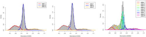
The computational feasibility and stability of the proposed algorithm allowed us to increase the value of N and perform model selection. Preliminary runs indicated that N > 5 was likely to be favored, so we used adSP with state-specific knots along with the marginal likelihood approach described above. Using a discrete uniform prior over $\{2,\dots ,10\}$, the posterior modal number of states was estimated to be N = 9, with a posterior probability of 1, thus the data strongly support a considerably larger number of states than was originally assumed in Langrock et al. (2018). In addition, individual emissions of the 9-state model now appear unimodal (see right panel of Figure 1). This is interesting: apart from investigating the biological interpretation of these states, our results suggest that one might consider fitting a fully parametric HMM with standard unimodal forms of emission densities for N = 9. Further detailed results of the application to the shark data can be found in supplementary Section D.

4.2 A Conditional HMM for Analysing Circadian and Sleep Patterns in Human PA Data

4.2.1 The Model

The use of PA data obtained from wearable sensors for monitoring circadian rhythm and sleep pattern outside laboratory settings is well justified (Ancoli-Israel et al. 2015; Quante et al. 2018). We next use our proposed Ansatz to introduce a conditional hidden Markov model in its general form and illustrate the method using publicly available human PA data from MESA. The conditional HMM consists of a “main model” to characterize the general pattern of the overall time series, and a “sub-HMM” that is invoked based on a specific state i of the main model with N_S possible sub-states. Without loss of generality, we set i = 1 and for simplicity omit this subscript in what follows. The posterior distribution of the parameters in the sub-HMM can be expressed as (7) $$f({\mathit{\theta }}^S|{\mathbf{y}}^{(n)})=\int f({\mathit{\theta }}^S|{\mathbf{x}}^{(n)},{\mathbf{y}}^{(n)})f({\mathbf{x}}^{(n)}|{\mathbf{y}}^{(n)})d{\mathbf{x}}^{(n)},$$(7) where ${\mathit{\theta }}^S$ is the parameter set for a N_S-state sub-HMM, ${\mathbf{x}}^{(n)}$ is the hidden state sequence associated with the main-HMM and we assume that (8) $$f({\mathit{\theta }}^S|{\mathbf{x}}^{(n)},{\mathbf{y}}^{(n)})\propto f({\mathit{\theta }}^S)f({\mathbf{y}}^{(n)}|{\mathit{\theta }}^S,{\mathbf{x}}^{(n)}).$$(8)

We refer to the second term in (8) as the “conditional likelihood” for the sub-HMM. The key idea here is that by conditioning on state 1 of the main-HMM, we want to restrict the observations that contribute to the likelihood to only those associated with the time points where x_t = 1, while also maintaining the temporal dependence of these observations. To achieve this, we could simply treat observations $\{y_t:x_t\ne 1\}$ as “missing data”. This strategy offers the advantage that the resulting conditional likelihood can be easily evaluated in the HMM framework. More specifically, let $(t_1,\dots ,t_{T_1})$ be the collection of time points in ascending order such that $x_{t_j}=1,j=1,\dots ,T_1$. Using the notation of Section 2, we have (9) $$\begin{array}{cc}f({\mathbf{y}}^{(n)}|{\mathit{\theta }}^S,{\mathbf{x}}^{(n)})\hfill & =f(y_{t_1},\dots ,y_{t_{T_1}}|{\mathit{\theta }}^S)\hfill \\ \hfill & =\sum _{x_{t_1},\dots ,x_{t_{T_1}}}f(y_{t_1},\dots ,y_{t_{T_1}},x_{t_1},\dots ,x_{t_{T_1}}|{\mathit{\theta }}^S)\hfill \\ \hfill & =\mathit{\delta }P(y_1)\Gamma P(y_2)\cdots \Gamma P(y_n)\mathbf{1}\hfill \end{array},$$(9) where $P(y_t)=I_{N_S}$, the identity matrix of dimension N_S, for $t\ne t_1,\dots ,t_{T_1}$. The last row of (9) takes the same form as the marginal likelihood of a standard HMM, and therefore, the standard forward algorithm can be used to efficiently evaluate the conditional likelihood. Note that the uncertainty regarding the state classification is properly taken into account, as the state sequence will be integrated out to obtain the marginal posterior as defined in (7), on which our inference for the sub-HMM will be based.

It should be pointed out that our conditional HMM approach is different from what is called the hierarchical HMM (see e.g., Adam et al. 2019) in that for the latter, a joint model is formulated for multiple observed processes at different temporal resolutions, each of which is modeled via a hidden Markov process and the process at the coarser level determines the onset of a specific finer level process for each epoch. In contrast, our method may operate on a single time scale and allows us to refine our analysis of a chosen state. It is also important to note that fitting the main HMM with $N+N_S-1$ states will not necessarily split state 1 of the original model into N_S sub-states as desired, whereas in our framework we control this directly through the conditioning.

In our application we are interested in studying sleep from accelerometer data, where state 1 corresponds to the lowest activity state that contains the sleep bouts. However, accelerometer data often contain a large number of zeros during a rest or sleep state (Ae Lee and Gill 2018), which could cause issues for the spline-based model. To address this, we assume a “zero inflation” of the emissions at both HMM levels⁷ $$f_{x_t}(y_t)=w_{x_t,1}{\delta }_0+w_{x_t,2}{f}_{x_t}^B(y_t),$$where x_t indicates the underlying state at time t, $w_{x_t,1}$ represents the state-specific zero weight such that $0\le w_{x_t,1}\le 1$ and $w_{x_t,1}+w_{x_t,2}=1$, δ₀ is the Dirac delta distribution and $f_{x_t}^B(y_t)$ is a spline-based emission density as defined in Section 2. Following Gassiat, Cleynen, and Robin (2016a) we can establish identifiability of the resulting HMM provided that at most one $w_{x_t,1}$ is equal to one and that $\{{\delta }_0,f_1^B,\dots ,f_N^B\}$ are linearly independent. In our analysis these conditions are always satisfied.

4.2.2 Application to the MESA Dataset

To illustrate our proposed method, we consider two example subjects, A and B, corresponding to subjects 921 and 3439 in the MESA dataset, respectively, who both have no diagnosed sleep related diseases. Subjects wore an actigraph (Actiwatch Spectrum) on the non-dominant wrist for one week and activity was measured in each 30-sec epoch by counting the number of times movement intensity crossed a threshold. The resulting values reflect the overall activity intensity in each epoch. Additionally, each subject undertook a polysomnography (PSG) session for one night during the monitoring period. PSG is a multi-sensor approach that collects multiple physiological signals from the body and is considered as the gold standard of measuring sleep (Berry et al. 2012). Wake and four sleep stages (N1, N2, N3, and REM) were identified for every 30-sec epoch using the criteria set out by the American Academy of Sleep Medicine. Among these, N1 and N3 correspond to light and deep sleep, respectively, while N2 is an intermediate stage. N1, N2, and N3 are collectively referred to as non-REM stages (Berry et al. 2012). The REM stage is physiologically distinct from the other stages and associated with dreaming (Stein and Pu 2012). Typically, individuals go through the four stages several times during a night’s sleep. For the main-HMM, we used 5-min averaged PA and set N = 3 as in Huang et al. (2018).⁸ For the sub-HMM we assume 2 sub-states, 1.1 and 1.2, to potentially capture the ultradian oscillations between higher and lower intensity of movement during sleep. Such were found in accelerometer data by Winnebeck et al. (2018) who concluded that they correspond to the circa 120-min periodic transitions between the Non-REM and REM stages of sleep. However, their Ansatz could not account for a stochastic oscillating pattern. We based inference for the sub-HMM on the finest possible time resolution of the raw 30-sec PA counts to focus on the detail of activity during sleep. The implementational details of the MCMC algorithm are provided in supplementary Section E.

The left panels of Figure 2 depict the 5-min averaged PA data for subjects A and B, along with the locally decoded states and the cumulative posterior probabilities of the three states at each time point (i.e., $P(x_t\le i|\widehat{\mathit{\theta }},{\mathbf{y}}^{(n)});i=1,2,3$) under the fitted main-HMMs. State 1 (in blue) is characterized by periods of immobility, usually occurring at night time. Other states (in pink and red shades) usually correspond to day-time activities of varying intensity, which depend on the subject’s lifestyle and may be interrupted by daytime naps, as seen for subject B. The estimated main-HMM suggests that subject A has a more active lifestyle and a more regular sleep-wake routine, with no significant sleep disruptions during the monitoring period. In contrast, subject B appears to suffer from a more disturbed circadian rhythm. These visual impressions are supported by estimating additional HMM-derived parameters that can be used to quantify an individual’s circadian rhythm, such as the dichotomy I < O and rhythm indices (computed as in Huang et al. 2018), where lower values indicate more disrupted circadian rhythms. For B, these values were 96.4% and 0.553 while A had higher values of 99.4% and 0.774, respectively. These findings are consistent with the sleep questionnaires completed by the subjects, where B reported having generally restless sleep and sometimes having trouble falling asleep. We also evaluated the performance of our main-HMM in classifying sleep (state 1) versus wake (states 2 and 3) by comparing its decoding output to PSG-derived sleep/wake labels (available for one night) on an epoch-by-epoch basis, where the PSG stage for each 5-min epoch are determined by the most frequent stage of the corresponding ten 30-sec bins in the raw PSG labels. Our main-HMM achieved state-of-the-art performance in terms of overall accuracy, sensitivity for sleep (proportion of true sleep epochs identified correctly) and specificity for wake (proportion of true wake epochs identified correctly), with values of 88.2%, 100%, 70.7% for subject A and 89.9%, 94.4%, and 79.5% for B, respectively. The relatively lower accuracy for detecting wake is expected as there are usually in-bed times before falling asleep or gentle sleep interruptions that are characterized by low or no activity. Our main-HMM provides useful quantitative summaries of an individual’s rest-activity profile, as proposed in a parametric approach in Huang et al. (2018), but with the added benefit of a more flexible modeling of the emissions. The parameter ${\widehat{\gamma }}_{1,1}$ is of particular interest for circadian and sleep analysis as low values suggest interrupted or fragmented sleep and thus a low quality of sleep, which is another indicator of circadian disruption. For subject B, the posterior mean for ${\gamma }_{1,1}$ was 0.916, which is lower than 0.98 obtained for subject A.

Fig. 2 Left: Results from main-HMM fitted to 5-min averaged PA data over a monitoring period of 7 days (Top panel: data with colors indicating the locally decoded state at each time; bottom panel: cumulative posterior probability of the state at each time, that is $P(x_t\le i|\mathit{\theta },{\mathbf{y}}^{(n)});i=1,2,3$). Right: Results of sub-HMM fitted to the 30-sec PA data, focusing on the one-night PSG monitoring period (Top panel: locally decoded state at each time; bottom panel: corresponding cumulative probability of each sub-state at each time. Data in red represent those assigned to states outside of state 1 by the local decoding result for the main-HMM).

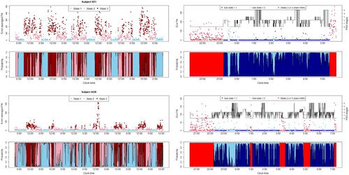
The right panels of Figure 2 show the locally decoded time series of the 30-sec PA data during the PSG monitoring period along with the cumulative probability of the two sub-states. As observed, for both subjects, the transitions between and the times spent in the two sub-states are highly stochastic. State 1.1 has a high probability of observing zero, with a posterior mean of zero weight ${\widehat{w}}_{1.1,1}$ of 0.908 and 0.963 for subjects A and B, while state 1.2 captures a moderately higher level of activity where the posterior mean ${\widehat{w}}_{1.2,1}$ for A and B are 0.325 and 0.463, respectively. To investigate the link between the sub-states in our HMM and the true sleep stages from PSG, we computed the proportion of the five PSG stages (wake, N1, N2, N3, REM) contained in each of the two HMM sub-states (see Table 1).⁹ We can see that while both sub-states contain a mix of all the PSG stages, only state 1.1 contained any deep sleep stages (N3) and had smaller proportions of wake and light sleep stages (N1) compared to state 1.2. This can also be seen by looking at the percentage of the PSG stages decoded as State 1.1, which are $(23.8\%,82.1\%,96.1\%,100\%,92.9\%)$ for subject A and $(26\%,67.4\%,77\%,100\%,67.9\%)$ for subject B for (wake, N1, N2, N3, REM). In contrast, State 1.2 tends to be associated with lighter sleep stages as well as disruptions into wake which were not identified by the main-HMM. We therefore anticipate that state 1.2 provides additional useful information regarding the sleep quality of a subject.

Table 1 Composition of the states of the sub-HMM with respect to PSG stages.

Subject	sub-state	Wake	N1	N2	N3	REM
Subject A	1.1	0.155	0.098	0.569	0.038	0.14
	1.2	0.568	0.162	0.176	0	0.095
Subject B	1.1	0.174	0.167	0.529	0.051	0.078
	1.2	0.264	0.224	0.398	0	0.114

The estimated transition probabilities of the fitted sub-HMM provide a systematic quantitative summary which could be used, for example, to compare sleep behaviour between subjects. For subject A, the diagonal entries of Γ have posterior means (±1 standard deviation) of ${\widehat{\gamma }}_{1.1,1.1}=0.966$ (±0.01) and ${\widehat{\gamma }}_{1.2,1.2}=0.665$ (±0.056), and those for subject B are ${\widehat{\gamma }}_{1.1,1.1}=0.908$ (±0.009) and ${\widehat{\gamma }}_{1.2,1.2}=0.727$ (±0.047). B has a lower ${\widehat{\gamma }}_{1.1,1.1}$ and higher ${\widehat{\gamma }}_{1.2,1.2}$, indicating a higher probability of leaving state 1.1 and a longer expected staying time in state 1.2, which may be associated with poorer sleep quality during the monitoring period. Indeed, according to the MESA database, subject B has a lower sleep efficiency 63.15% (computed from PSG) compared to 66.37% for A. Our results are also consistent with Table 2, which shows that subject B spent a larger proportion of sleep time in wake and N1 stages while having a lower proportion of time in the deeper N2 and N3 stages. The decoding and state probabilities of the sub-HMM also allow us to investigate the dynamic variation within and between bouts of sleep. For instance, the fragmentation of the blue region in the state probability plots of Figure 2 suggests that subject A seems to experience more interruptions and lighter sleep during the earlier phase of the sleep bout, whereas subject B suffers from sleep interruptions and transitions to lighter sleep throughout the entire bout. These observations are consistent with their own reports in the sleep questionnaire and the PSG recordings during the single night.

Table 2 Proportions of time spent in different PSG stages during sleep for the example subjects.

Subject	Wake	N1	N2	N3	REM
Subject A	0.21	0.105	0.519	0.035	0.132
Subject B	0.369	0.143	0.394	0.03	0.066

5 Summary and Further Discussion

In this article, we propose and develop a Bayesian methodology for inference in spline-based HMMs, which offer attractive properties compared to alternative nonparametric HMMs in terms of simplicity in model interpretation and flexibility in modeling. Our method allows for the number of states, N, to be unknown along with all other model parameters including the spline knot configuration(s). Compared with a P-spline-based construction, we achieve a parsimonious and efficient positioning of the spline knots via a RJMCMC algorithm, where the knots can either be shared across states or be state-specific. Model selection on N is based on the marginal likelihood, which can be effectively estimated via a truncated harmonic mean estimator under an easy-to-implement parallel sampling scheme. Through extensive simulation studies, we demonstrated the effectiveness and superiority of our proposed methods over alternative comparators, including the Gaussian mixture based HMM, the frequentist P-spline-based approach of Langrock et al. (2015), and a Bayesian adaptive P-spline approach which is investigated here for the first time. Importantly, the computational efficiency and flexibility of our algorithm allows us to deal with more states, which is a challenging problem even for parametric approaches due to convergence problems with increasing N. We highlight this advantage in the application to the animal movement data and illustrate the use of our method as a nonparametric approach for explorative data analysis.

The application to human PA data highlights the flexibility of our Bayesian modeling approach that can be extended in a relatively straightforward way to hierarchical scenarios such as the conditional HMM. The extension to a hierarchical framework of a sub-HMM within an overall HMM here allows us to estimate many important parameters that characterize an individual’s circadian rhythm, and to model the individual stochastic dynamics of the rest state activity where the sub-states may be associated with deeper and lighter or interrupted sleep stages. Another feature of our method is that the algorithm operates in an unsupervised manner, that is it does not require PSG labels for learning the model, which is desirable in applied settings as these labels are very costly or even impossible to acquire (Li et al. 2020). The method developed here is thus of imminent interest to sleep and circadian biology researchers using data from wearable sensors.

Our modeling framework opens up several possible extensions in further research. For instance, the homogeneous assumption on the hidden Markov chain can be relaxed by reparameterizing Γ in terms of the covariates via multinomial logistic link functions (Zucchini, MacDonald, and Langrock 2016). Efficient MCMC inference can be achieved by incorporating the Polya-Gamma data augmentation scheme of Polson, Scott, and Windle (2013), which was successfully applied to parametric nonhomogeneous HMMs in Holsclaw et al. (2017), into the present modeling framework. Our methodology can also be extended in a relatively straightforward manner to Markov switching (generalized) additive models as studied in Langrock et al. (2017, 2018) using frequentist approaches, where the splines can be used to model the functional effects of the covariates instead of the emissions. Without the density constraints on the spline parameters, the design of the RJMCMC algorithm can be simplified, and the efficiency of the resulting algorithm may be further improved. We believe that the advantages of using a Bayesian approach over a frequentist penalized approach as observed in this article would carry over to this context. Additionally, it would be interesting to explore the combination of the modern deep-learning-based methods, which excel at handling highly complex temporal dependence in the series and using historical information sets, with the conventional HMM probabilistic framework for achieving better predictive ability while maintaining model interpretability.

Supplementary Materials

Supplementary document: Provides additional details and results related to the proposed methods, simulation studies, and case studies. (.pdf file)

Code: Contains the code used in the simulation studies and case studies. (.zip file)

Acknowledgments

We wish to thank Prof. Roland Langrock, Dr. Yannis Papastamatiou and Dr. Yuuki Watanabe for providing the Oceanic Whitetip shark data. We wish to acknowledge Dr. Qi Huang for her support on the analysis of human accelerometer data. We would also like to acknowledge the Warwick Statistics Department and MRC Biostatistics Unit, University of Cambridge for the support of Sida Chen’s research. We are grateful to the editors and the reviewers for their constructive comments that have significantly improved the manuscript.

Disclosure Statement

The authors declare no competing financial or nonfinancial interests.

Additional information

Funding

The authors received no external funding for this research.

Notes

1 We refer to Chen et al. (2015) and Zhang et al. (2018) for more background information on the MESA dataset.

2 Clearly larger default values, including the sample size n, may be used instead and the estimation results do not appear to be sensitive to its choice as long as $K_{\max }$ is large enough.

3 In our experiments we did not find the values of these hyperparameters to be very influential, and other reasonable values may be used.

4 Note that it is not possible to estimate it consistently as there is only one unobserved variable associated with it.

5 We note the difference between our birth and death proposals to those in Sharef et al. (2010) (see eq. 3.1(3) $$\begin{array}{cc}f({\mathbf{y}}^{(n)}|K,R_K,\mathit{\delta },A_K,\Gamma )\hfill & =\int f({\mathbf{y}}^{(n)},{\mathbf{x}}^{(n)}|K,R_K,\mathit{\delta },A_K,\Gamma )d{\mathbf{x}}^{(n)}\hfill \\ \hfill & =\mathit{\delta }P(y_1)\Gamma P(y_2)\cdots \Gamma P(y_n)\mathbf{1},\hfill \end{array}$$(3) therein), who propose a parameterization where the transformation acts on the exponentials of the spline coefficients (restricted to be positive). Such a scheme may be problematic as the proposed parameters from the death step based on the deterministic rules are not guaranteed to be positive.

6 This finding is consistent with our experience in the simulation studies.

7 The model can be easily adapted to applications where further discrete mass points for low observations are needed.

8 One could first perform model selection with the marginal method introduced earlier. However, for comparison and since model selection is not the main theme of this application we use the settings of Huang et al. (2018). They found that N = 3 tended to be the optimal choice in parametric HMM modeling of this kind of data, which, furthermore, consistently over many individuals, assigned the rest/sleep periods to night times

9 Here we present only results for our two example subjects. Such an analysis could be extended to include all MESA subjects but this is beyond the remit of this article.

References

- Acerbi, L., Dokka, K., Angelaki, D. E., and Ma, W. J. (2018), “Bayesian Comparison of Explicit and Implicit Causal Inference Strategies in Multisensory Heading Perception,” PLoS Computational Biology, 14, e1006110. DOI: 10.1371/journal.pcbi.1006110.
- Adam, T., Griffiths, C. A., Leos-Barajas, V., Meese, E. N., Lowe, C. G., Blackwell, P. G., Righton, D., and Langrock, R. (2019), “Joint Modelling of Multi-Scale Animal Movement Data Using Hierarchical Hidden Markov Models,” Methods in Ecology and Evolution, 10, 1536–1550. DOI: 10.1111/2041-210X.13241.
- Ae Lee, J., and Gill, J. (2018), “Missing Value Imputation for Physical Activity Data Measured by Accelerometer,” Statistical Methods in Medical Research, 27, 490–506. DOI: 10.1177/0962280216633248.
- Alexandrovich, G., Holzmann, H., and Leister, A. (2016), “Nonparametric Identification and Maximum Likelihood Estimation for Hidden Markov Models,” Biometrika, 103, 423–434. DOI: 10.1093/biomet/asw001.
- Ancoli-Israel, S., Martin, J. L., Blackwell, T., Buenaver, L., Liu, L., Meltzer, L. J., Sadeh, A., Spira, A. P., and Taylor, D. J. (2015), “The SBSM Guide to Actigraphy Monitoring: Clinical and Research Applications,” Behavioral Sleep Medicine, 13, S4–S38. DOI: 10.1080/15402002.2015.1046356.
- Atchade, Y., Fort, G., Moulines, E., and Priouret, P. (2011), “Adaptive Markov Chain Monte Carlo: Theory and Methods,” Bayesian Time Series Models, eds. D. Barber, A. Taylan Cemgil, and S. Chiappa, pp. 32–47, New York: Cambridge University Press.
- Baudry, J.-P., and Celeux, G. (2015), “EM for Mixtures,” Statistics and Computing, 25, 713–726. DOI: 10.1007/s11222-015-9561-x.
- Berry, R. B., Brooks, R., Gamaldo, C. E., Harding, S. M., Marcus, C., Vaughn, B. V., et al. (2012), “The AASM Manual for the Scoring of Sleep and Associated Events,” Rules, Terminology and Technical Specifications, Darien, Illinois, American Academy of Sleep Medicine, 176, 2012.
- Brooks, S. P., Giudici, P., and Roberts, G. O. (2003), “Efficient Construction of Reversible Jump Markov Chain Monte Carlo Proposal Distributions,” Journal of the Royal Statistical Society, Series B, 65, 3–39. DOI: 10.1111/1467-9868.03711.
- Cappé, O., Moulines, E., and Rydén, T. (2005), Inference in Hidden Markov Models, New York: Springer.
- Cappé, O., Robert, C. P., and Rydén, T. (2003), “Reversible Jump, Birth-and-Death and More General Continuous Time Markov Chain Monte Carlo Samplers,” Journal of the Royal Statistical Society, Series B, 65, 679–700. DOI: 10.1111/1467-9868.00409.
- Carlin, B. P., and Chib, S. (1995), “Bayesian Model Choice via Markov Chain Monte Carlo Methods,” Journal of the Royal Statistical Society, Series B, 57, 473–484. DOI: 10.1111/j.2517-6161.1995.tb02042.x.
- Celeux, G., and Durand, J.-B. (2008), “Selecting Hidden Markov Model State Number With Cross-Validated Likelihood,” Computational Statistics, 23, 541–564. DOI: 10.1007/s00180-007-0097-1.
- Chen, X., Wang, R., Zee, P., Lutsey, P. L., Javaheri, S., Alcántara, C., Jackson, C. L., Williams, M. A., and Redline, S. (2015), “Racial/Ethnic Differences in Sleep Disturbances: The Multi-Ethnic Study of Atherosclerosis (MESA),” Sleep, 38, 877–888. DOI: 10.5665/sleep.4732.
- De Boor, C. (2001), A Practical Guide to Splines, Applied Mathematical Sciences, New York: Springer.
- De Boor, C., De Boor, C., Mathématicien, E.-U., De Boor, C., and De Boor, C. (1978). A Practical Guide to Splines (Vol. 27), New York: Springer-Verlag.
- De Castro, Y., Gassiat, E., and Le Corff, S. (2017), “Consistent Estimation of the Filtering and Marginal Smoothing Distributions in Nonparametric Hidden Markov Models,” IEEE Transactions on Information Theory, 63, 4758–4777. DOI: 10.1109/TIT.2017.2696959.
- Denison, D. G., Holmes, C. C., Mallick, B. K., and Smith, A. F. (2002), Bayesian Methods for Nonlinear Classification and Regression (Vol. 386), Chichester: Wiley.
- DiCiccio, T. J., Kass, R. E., Raftery, A., and Wasserman, L. (1997), “Computing Bayes Factors by Combining Simulation and Asymptotic Approximations,” Journal of the American Statistical Association, 92, 903–915. DOI: 10.1080/01621459.1997.10474045.
- DiMatteo, I., Genovese, C. R., and Kass, R. E. (2001), “Bayesian Curve-Fitting with Free-Knot Splines,” Biometrika, 88, 1055–1071. DOI: 10.1093/biomet/88.4.1055.
- Durmus, A., Moulines, E., and Pereyra, M. (2018), “Efficient Bayesian Computation by Proximal Markov Chain Monte Carlo: When Langevin Meets Moreau,” SIAM Journal on Imaging Sciences, 11, 473–506. DOI: 10.1137/16M1108340.
- Edwards, M. C., Meyer, R., and Christensen, N. (2019), “Bayesian Nonparametric Spectral Density Estimation Using b-spline Priors,” Statistics and Computing, 29, 67–78. DOI: 10.1007/s11222-017-9796-9.
- Fan, W., Wang, R., and Bouguila, N. (2021), “Simultaneous Positive Sequential Vectors Modeling and Unsupervised Feature Selection via Continuous Hidden Markov Models,” Pattern Recognition, 119, 108073. DOI: 10.1016/j.patcog.2021.108073.
- Fox, E. B., Sudderth, E. B., Jordan, M. I., and Willsky, A. S. (2011), “A Sticky HDP-HMM with Application to Speaker Diarization,” The Annals of Applied Statistics, 5, 1020–1056. DOI: 10.1214/10-AOAS395.
- Friedman, J., Hastie, T., and Tibshirani, R. (2001), The Elements of Statistical Learning, Springer Series in Statistics (Vol. 1), New York, Springer.
- Friel, N., and Wyse, J. (2012), “Estimating the Evidence–A Review,” Statistica Neerlandica, 66, 288–308. DOI: 10.1111/j.1467-9574.2011.00515.x.
- Frühwirth-Schnatter, S., and Frèuhwirth-Schnatter, S. (2006), Finite Mixture and Markov Switching Models (Vol. 425), New York: Springer.
- Gassiat, É., Cleynen, A., and Robin, S. (2016a), “Inference in Finite State Space Non Parametric Hidden Markov Models and Applications,” Statistics and Computing, 26, 61–71. DOI: 10.1007/s11222-014-9523-8.
- Gassiat, E., and Rousseau, J. (2016b), “Nonparametric Finite Translation Hidden Markov Models and Extensions,” Bernoulli, 22, 193–212. DOI: 10.3150/14-BEJ631.
- Gelfand, A. E., and Dey, D. K. (1994), “Bayesian Model Choice: Asymptotics and Exact Calculations,” Journal of the Royal Statistical Society, Series B, 56, 501–514. DOI: 10.1111/j.2517-6161.1994.tb01996.x.
- Green, P. J. (1995), “Reversible Jump Markov Chain Monte Carlo Computation and Bayesian Model Determination,” Biometrika, 82, 711–732. DOI: 10.1093/biomet/82.4.711.
- Hastie, D. I., Liverani, S., and Richardson, S. (2015), “Sampling from Dirichlet Process Mixture Models with Unknown Concentration Parameter: Mixing Issues in Large Data Implementations,” Statistics and Computing, 25, 1023–1037. DOI: 10.1007/s11222-014-9471-3.
- Holsclaw, T., Greene, A. M., Robertson, A. W., and Smyth, P. (2017), “Bayesian Nonhomogeneous Markov Models via Pólya-Gamma Data Augmentation with Applications to Rainfall Modeling,” The Annals of Applied Statistics, 11, 393–426. DOI: 10.1214/16-AOAS1009.
- Huang, Q., Cohen, D., Komarzynski, S., Li, X.-M., Innominato, P., Lévi, F., and Finkenstädt, B. (2018), “Hidden Markov Models for Monitoring Circadian Rhythmicity in Telemetric Activity Data,” Journal of The Royal Society Interface, 15, 20170885. DOI: 10.1098/rsif.2017.0885.
- Kang, K., Cai, J., Song, X., and Zhu, H. (2019), “Bayesian Hidden Markov Models for Delineating the Pathology of Alzheimer’s Disease,” Statistical Methods in Medical Research, 28, 2112–2124. DOI: 10.1177/0962280217748675.
- Koo, J.-Y. (1996), “Bivariate b-splines for Tensor Logspline Density Estimation,” Computational Statistics & Data Analysis, 21, 31–42. DOI: 10.1016/0167-9473(95)00003-8.
- Lang, S., and Brezger, A. (2004), “Bayesian p-Splines,” Journal of Computational and Graphical Statistics, 13, 183–212. DOI: 10.1198/1061860043010.
- Langrock, R., Adam, T., Leos-Barajas, V., Mews, S., Miller, D. L., and Papastamatiou, Y. P. (2018), “Spline-based Nonparametric Inference in General State-Switching Models,” Statistica Neerlandica, 72, 179–200. DOI: 10.1111/stan.12133.
- Langrock, R., King, R., Matthiopoulos, J., Thomas, L., Fortin, D., and Morales, J. M. (2012), “Flexible and Practical Modeling of Animal Telemetry Data: Hidden Markov Models and Extensions,” Ecology, 93, 2336–2342. DOI: 10.1890/11-2241.1.
- Langrock, R., Kneib, T., Glennie, R., and Michelot, T. (2017), “Markov-Switching Generalized Additive Models,” Statistics and Computing, 27, 259–270. DOI: 10.1007/s11222-015-9620-3.
- Langrock, R., Kneib, T., Sohn, A., and DeRuiter, S. L. (2015), “Nonparametric Inference in Hidden Markov Models Using p-splines,” Biometrics, 71, 520–528. DOI: 10.1111/biom.12282.
- Lehéricy, L. (2018), “State-by-State Minimax Adaptive Estimation for Nonparametric Hidden Markov Models,” The Journal of Machine Learning Research, 19, 1432–1477.
- Lehéricy, L. (2019), “Consistent Order Estimation for Nonparametric Hidden Markov Models,” Bernoulli, 25, 464–498. DOI: 10.3150/17-BEJ993.
- Li, X., Zhang, Y., Jiang, F., and Zhao, H. (2020), “A Novel Machine Learning Unsupervised Algorithm for Sleep/Wake Identification Using Actigraphy,” Chronobiology International, 37, 1002–1015. DOI: 10.1080/07420528.2020.1754848.
- Llorente, F., Martino, L., Delgado, D., and Lopez-Santiago, J. (2020), “Marginal Likelihood Computation for Model Selection and Hypothesis Testing: An Extensive Review,” arXiv preprint arXiv:2005.08334.
- Marin, J.-M., and Robert, C. P. (2009), “Importance Sampling Methods for Bayesian Discrimination between Embedded Models,” arXiv preprint arXiv:0910.2325.
- Piccardi, M., and Pérez, Ó. (2007), “Hidden Markov Models with Kernel Density Estimation of Emission Probabilities and their Use in Activity Recognition,” in CVPR, Citeseer.
- Pohle, J., Langrock, R., van Beest, F. M., and Schmidt, N. M. (2017), “Selecting the Number of States in Hidden Markov Models: Pragmatic Solutions Illustrated Using Animal Movement,” Journal of Agricultural, Biological and Environmental Statistics, 22, 270–293. DOI: 10.1007/s13253-017-0283-8.
- Polson, N. G., Scott, J. G., and Windle, J. (2013), “Bayesian Inference for Logistic Models Using Pólya–Gamma Latent Variables,” Journal of the American statistical Association, 108, 1339–1349. DOI: 10.1080/01621459.2013.829001.
- Quante, M., Kaplan, E. R., Cailler, M., Rueschman, M., Wang, R., Weng, J., Taveras, E. M., and Redline, S. (2018), “Actigraphy-based Sleep Estimation in Adolescents and Adults: A Comparison with Polysomnography Using Two Scoring Algorithms,” Nature and Science of Sleep, 10, 13–20. DOI: 10.2147/NSS.S151085.
- Rabiner, L. R. (1989), “A Tutorial on Hidden Markov Models and Selected Applications in Speech Recognition,” Proceedings of the IEEE, 77, 257–286. DOI: 10.1109/5.18626.
- Robert, C. P., and Wraith, D. (2009), “Computational Methods for Bayesian Model Choice,” AIP Conference Proceedings 1193, 251–262.
- Roenneberg, T., and Merrow, M. (2016), “The Circadian Clock and Hhuman Health,” Current Biology, 26, R432–R443. DOI: 10.1016/j.cub.2016.04.011.
- Rydén, T. (2008), “EM versus Markov Chain Monte Carlo for Estimation of Hidden Markov Models: A Computational Perspective,” Bayesian Analysis, 3, 659–688. DOI: 10.1214/08-BA326.
- Schumaker, L. (2007). Spline Functions: Basic Theory, Cambridge: Cambridge University Press.
- Sharef, E., Strawderman, R. L., Ruppert, D., Cowen, M., Halasyamani, L., et al. (2010), “Bayesian Adaptive b-spline Estimation in Proportional Hazards Frailty Models,” Electronic Journal of Statistics, 4, 606–642. DOI: 10.1214/10-EJS566.
- Stein, P. K., and Pu, Y. (2012), “Heart Rate Variability, Sleep and Sleep Disorders,” Sleep Medicine Reviews, 16, 47–66. DOI: 10.1016/j.smrv.2011.02.005.
- Vernet, E. (2015), “Posterior Consistency for Nonparametric Hidden Markov Models with Finite State Space,” Electronic Journal of Statistics, 9, 717–752. DOI: 10.1214/15-EJS1017.
- Volant, S., Bérard, C., Martin-Magniette, M.-L., and Robin, S. (2014), “Hidden Markov Models with Mixtures as Emission Distributions,” Statistics and Computing, 24, 493–504. DOI: 10.1007/s11222-013-9383-7.
- Winnebeck, E. C., Fischer, D., Leise, T., and Roenneberg, T. (2018), “Dynamics and Ultradian Structure of Human Sleep in Real Life,” Current Biology, 28, 49–59. DOI: 10.1016/j.cub.2017.11.063.
- Yau, C., Papaspiliopoulos, O., Roberts, G. O., and Holmes, C. (2011), “Bayesian Non-parametric Hidden Markov Models with Applications in Genomics,” Journal of the Royal Statistical Society, Series B, 73, 37–57. DOI: 10.1111/j.1467-9868.2010.00756.x.
- Zanini, E., Eastoe, E., Jones, M., Randell, D., and Jonathan, P. (2020), “Flexible Covariate Representations for Extremes,” Environmetrics, 31, e2624. DOI: 10.1002/env.2624.
- Zhang, G.-Q., Cui, L., Mueller, R., Tao, S., Kim, M., Rueschman, M., Mariani, S., Mobley, D., and Redline, S. (2018), “The National Sleep Research Resource: Towards a Sleep Data Commons,” Journal of the American Medical Informatics Association, 25, 1351–1358. DOI: 10.1093/jamia/ocy064.
- Zucchini, W., MacDonald, I. L., and Langrock, R. (2016), Hidden Markov Models for Time Series: An Introduction Using R, Boca Raton, FL: Chapman and Hall/CRC.