Dissecting Gene Expression Heterogeneity: Generalized Pearson Correlation Squares and the K-Lines Clustering Algorithm

Abstract

Motivated by the pressing needs for dissecting heterogeneous relationships in gene expression data, here we generalize the squared Pearson correlation to capture a mixture of linear dependences between two real-valued variables, with or without an index variable that specifies the line memberships. We construct the generalized Pearson correlation squares by focusing on three aspects: variable exchangeability, no parametric model assumptions, and inference of population-level parameters. To compute the generalized Pearson correlation square from a sample without a line-membership specification, we develop a K-lines clustering algorithm to find K clusters that exhibit distinct linear dependences, where K can be chosen in a data-adaptive way. To infer the population-level generalized Pearson correlation squares, we derive the asymptotic distributions of the sample-level statistics to enable efficient statistical inference. Simulation studies verify the theoretical results and show the power advantage of the generalized Pearson correlation squares in capturing mixtures of linear dependences. Gene expression data analyses demonstrate the effectiveness of the generalized Pearson correlation squares and the K-lines clustering algorithm in dissecting complex but interpretable relationships. The estimation and inference procedures are implemented in the R package gR2 (https://github.com/lijy03/gR2). Supplementary materials for this article are available online, including a standardized description of the materials available for reproducing the work.

KEYWORDS:

• Asymptotic distribution
• Mixture of linear dependences
• Specified and unspecified generalized Pearson correlation squares

1 Introduction

In biomedical research, Pearson correlation and its rank-based variant Spearman correlation remain the most widely used association measures for describing the relationship between two scalar-valued variables, for example, two genes’ expression levels. The reason underlying the two measures’ popularity is 2-fold: linear and monotone relationships¹ are widespread in nature and interpretable to researchers. In many cases, however, the interesting relationship between two variables often depends on another hidden categorical variable.

For example, in a gene expression dataset of Arabidopsis thaliana, a plant model organism, many genes exhibit different linear dependences between root and shoot tissues (Li et al. 2008; Kim et al. 2012). Figure 1(A) shows pairwise relationships of flavin-monooxygenase (FMO) genes’ expression levels, and all these relationships differ between root and shoot tissues. In particular, FMO GS-OX2 and FMO GS-OX5 exhibit a positive (sample-level Pearson) correlation in shoots (black dots) but a negative correlation in roots (gray circles). Imagine an idealistic, extreme scenario (Figure 1(B)) where two genes have a positive (population-level Pearson) correlation $\rho \in (0,1)$ in the shoot tissue but a negative correlation $-\rho$ in the root tissue, and the two tissues are equally sampled; then the two genes would have a zero correlation if not conditional on the tissue.

Fig. 1 A: Pairwise expression levels of A. thaliana genes. B: A simulated toy example. Gray circles and black dots indicate data from root and shoot tissues, respectively.

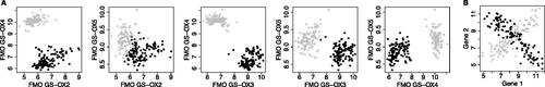
Real scenarios are usually not so extreme, but many of them exhibit a mixture relationship composed of two linear dependences (Li 2002), and they may show the “Simpson’s Paradox” where the overall correlation and the conditional correlations have opposite signs. Under such scenarios, Pearson correlation is a misleading measure, as it specifically looks for a single linear dependence. These scenarios often lack an index variable (e.g., the shoot/root tissue type) that segregates observations into distinct linear relationships. Moreover, numerous variable pairs (e.g.,10⁸ gene pairs) often need to be examined to discover unknown, but interesting and interpretable associations. Therefore, an association measure is in much demand to capture such relationships that are decomposable into a (possibly unknown) number of linear dependences, in a powerful and efficient way.

In the literature of scalar-valued association measures (also known as dependence measures), many measures have been developed to capture dependent relationships more general than the linear dependence. The first type of measures aims to capture more general functional (i.e., one-to-one) relationships. For monotone relationships, the Spearman’s rank correlation and the Kendall’s τ are commonly used. For functional relationships more general than monotonicity, there are measures including the maximal correlation efficient, measures based on nonparametric estimation of correlation curves (Bjerve and Doksum 1993) or principal curves (Delicado and Smrekar 2009), generalized measures of correlation that deals with asymmetrically explained variances and nonlinear relationships (Zheng, Shi, and Zhang 2012), measures for detecting local monotone patterns using count statistics (Wang, Waterman, and Huang 2014), the G² statistic derived from a regularized likelihood ratio test for piecewise-linear relationships (Wang, Jiang, and Liu 2017), and the recently proposed Chatterjee’s rank correlation ξ (Chatterjee 2021). The second type of measures aims to capture general dependence so that they only give zero values to independent random variable pairs. Examples include the maximal correlation coefficient and Chatterjee’s rank correlation ξ, which also belong to the first type, and other measures including the Hoeffding’s D, the mutual information, kernel-based measures such as the Hilbert-Schmidt Independence Criterion (HSIC) (Gretton et al. 2005), the distance correlation (Székely, Rizzo, and Bakirov 2007; Székely and Rizzo 2009) and its generalization as the multiscale graph correlation (MGC) (Shen, Priebe, and Vogelstein 2019), the maximal information coefficient (Reshef et al. 2011), the Heller-Heller-Gorfine (HHG) association test statistic based on ranks of distances (Heller, Heller, and Gorfine 2012), and the semiparametric kernel independence test for handling excess zeros (Lee and Zhu 2021). Specifically, the following measures are not restricted to comparing real-valued random variables: the Hoeffding’s D, the mutual information, the HSIC, the HHG test statistic, the distance correlation, and the MGC, among which the first four measures have the range $[0,\infty )$ instead of having absolute values under 1.

The aforementioned two types of measures have complementary advantages and disadvantages. Measures of the first type are generally interpretable but cannot capture the widespread nonfunctional (i.e., not one-to-one) relationships. In contrast, measures of the second type, though being versatile and having desirable theoretical properties, do not provide a straightforward interpretation of their captured relationships. As Figure 1 shows, many relationships are decomposable into a small number of linear dependences. Since the linear dependence is the simplest and most interpretable relationship, a mixture of a small number of linear dependences is also interpretable and often of great interest in biomedical research. For example, if researchers observe that a gene positively regulates a vital cancer gene in one cancer subtype but exhibits adverse regulatory effects in another subtype, different treatment strategies may be designed for the two cancer subtypes. However, mixtures of linear dependences remain challenging to capture: they are often missed by the first type of measures and cannot be distinguished from other less interpretable relationships by the second type of measures. Although mixtures of linear regression models have been of broad interest in fields including statistics, economics, social sciences, and machine learning for over 40 years (Quandt and Ramsey 1978; Murtaph and Raftery 1984; De Veaux 1989; Jacobs et al. 1991; Jones and McLachlan 1992; Wedel and DeSarbo 1994; Turner 2000; Hawkins, Allen, and Stromberg 2001; Hurn, Justel, and Robert 2003; Leisch 2008; Benaglia et al. 2009; Scharl, Grün, and Leisch 2009), they did not propose an association measure to capture mixtures of linear dependences, and neither do they trivially lead to a reasonable association measure, as we will explain below.

In this work, we propose generalized Pearson correlation squares, for which the squared Pearson correlation is a special case, to capture a mixture of linear dependences. Our proposal addresses the practical need to screen variable pairs that exhibit complex yet interpretable relationships. These relationships can be decomposed into linear components, where at least one component demonstrates statistical significance. We consider two scenarios: the specified scenario where an index variable indicates the line membership of each observation, and the more common unspecified scenario where no index variable is available. Under the specified scenario, we aim for our new measure to quantify the “informativeness” of the index variable, indicating whether it specifies distinct linear relationships. To achieve a reasonable generalization of the Pearson correlation, our new measures adhere to an essential property embraced by most existing association measures—the exchangeability of the two variables.² Additionally, we seek to provide both population-level parameters and sample-level statistics for our measures, enabling statistical inference and the assessment of statistical significance for observed measure values.

First, under the unspecified scenario, can we directly use the existing work on mixtures of linear regression models? The answer is no because these models require a specification of the response and predictor variables; that is, they do not consider the two variables symmetric. Except for the degenerate case where only one linear component exists, that is, the linear model, these models do not lead to a measure exchangeable for the two variables.

Second, still under the unspecified scenario, how to assign observations to lines to ensure the exchangeability? A good assignment should be able to handle general cases where observations from each line do not follow a specific distribution (as is required by model-based clustering) or have a spherical shape (as is required by the K-means clustering). To handle such cases, we propose the K-lines clustering algorithm in Section 2.2.1.

Third, how to define population-level measures to enable proper inference? A critical point is that the specified and unspecified scenarios need different population-level measures; otherwise, it would be impossible to construct unbiased estimators for both scenarios without distributional assumptions. We will elaborate on this point in Section 3.

Fourth, when an index variable is available, should we always use it to specify line memberships? Surprisingly, the answer is no because the index variable may be uninformative or irrelevant to the segregation of lines. In that case, it can be more informative to directly estimate line memberships from data by clustering. We will demonstrate this point using real data in Section 5.1.

This article is organized as follows. In Section 2, we define generalized Pearson correlation squares at the population and sample levels, under the line-membership specified and unspecified scenarios. For the unspecified scenario, we develop a K-lines clustering algorithm, following the subspace clustering literature (Vidal 2010). In Section 3, we derive the asymptotic distributions of the corresponding sample-level measures to enable efficient statistical inference. In Section 4, we conduct simulation studies under various settings to verify the asymptotic distributions and evaluate the finite-sample statistical power of the proposed measures. In Section 5, we demonstrate the use of the generalized Pearson correlation squares and the K-lines clustering algorithm for dissecting gene expression heterogeneity in two real datasets, followed by discussions in Section 6. Supplementary material includes all the proofs of lemmas and theorems, convergence properties of the K-lines algorithm, more simulation results, another real data application, real data description, more tables and figures, and additional references.

2 Generalized Pearson Correlation Squares and K-Lines Clustering Algorithm

The Pearson correlation is the most widely used measure to describe the relationship between two random variables $X,Y\in R$. At the population level, the Pearson correlation of X and Y is defined as $\rho =\text{cov}(X,Y)/{\{\text{var}(X)\text{var}(Y)\}}^{-1/2}\in [-1,1]$, where $\text{cov}(X,Y)=E[\{X-E(X)\left\}\right\{Y-E(Y)\}],\text{ var}(X)=E\left\{{[X-E(X)]}^2\right\}$, and $\text{var}(Y)=E\left\{{[Y-E(Y)]}^2\right\}$ denote the covariance between X and Y, the variance of X, and the variance of Y, respectively. We say that X and Y are linearly dependent if $\rho \ne 0$.

At the sample level, the Pearson correlation $R=\{{\sum }_{i=1}^n(X_i-\overline{X})(Y_i-\overline{Y})\}/{\left\{{\sum }_{i=1}^n{(X_i-\overline{X})}^2{\sum }_{i=1}^n{(Y_i-\overline{Y})}^2\right\}}^{1/2}$ is defined based on a sample ${\{(X_i,Y_i)\}}_{i=1}^n$ from the joint distribution of (X, Y), where $\overline{X}=n^{-1}{\sum }_{i=1}^n{X}_i$ and $\overline{Y}=n^{-1}{\sum }_{i=1}^n{Y}_i$. Motivated by the fact that R², the Pearson correlation square, is commonly used to describe the observed linear dependence in a bivariate sample, we develop generalized Pearson correlation squares to capture a mixture of linear dependences.

We define the line-membership specified scenario as the case where we also observe an index random variable $Z\in \{1,\dots ,K\}$ that specifies the linear dependence between X and Y, and K is the number of linear dependences. In parallel, we define the line-membership unspecified scenario as the case where no index variable is available. In the special case of K = 1, we have $Z\equiv 1$.

There may exist more than one index variable, and correspondingly there could be multiple specified scenarios. For example, in the A. thaliana gene expression dataset (Table S4 in the supplementary material), there are four index variables (condition, treatment, replicate, and tissue) that correspond to four different specified scenarios. As we will show in Section 5.1, only the tissue specification leads to a reasonable separation of linear relationships (Figures 1 and S5–S8 in the supplementary material). Hence, a specified scenario is not always preferred to the unspecified scenario when the goal is to capture an informative mixture of linear dependences.

2.1 Line-Membership Specified Scenario

2.1.1 Population-Level Generalized Pearson Correlation Square (Specified)

As the index variable Z is observable under the line-membership specified scenario, we denote $p_{\mathit{\text{kS}}}=P(Z=k),k=1,\dots ,K$. Conditional on Z = k, the population-level Pearson correlation between X and Y is ${\rho }_{\mathit{\text{kS}}}=\text{cov}(X,Y|Z=k)/{\{\text{var}(X|Z=k)\text{var}(Y|Z=k)\}}^{1/2}$, if $\text{var}(X|Z=k)>0$ and $\text{var}(Y|Z=k)>0$; otherwise, ${\rho }_{\mathit{\text{kS}}}=0$. In the special case of K = 1, ${\rho }_{1S}^2={\rho }^2={\text{cov}}^2(X,Y)/\{\text{var}(X)\text{var}(Y)\}$ is the population-level Pearson correlation square that indicates the population-level strength of a linear dependence. Motivated by this, we combine ${\rho }_{1S}^2,\dots ,{\rho }_{\mathit{\text{KS}}}^2$ into one measure to indicate the overall strength of K linear dependences.

Definition 2.1.

At the population level, when the line membership variable Z is specified, the generalized Pearson correlation square between X and Y is defined as (2.1) $${\rho }_{\mathit{\text{GS}}}^2=E_Z\left({\rho }_{\mathit{\text{ZS}}}^2\right)=E_Z\left\{\frac{{\text{cov}}^2(X,Y|Z)}{\text{var}(X|Z)\text{var}(Y|Z)}\right\}=\sum _{k=1}^K{p}_{\mathit{\text{kS}}}{\rho }_{\mathit{\text{kS}}}^2,$$(2.1) a weighted sum of ${\rho }_{1S}^2,\dots ,{\rho }_{\mathit{\text{KS}}}^2$, that is, the strengths of the K linear dependences, with weights as $p_{1S},\dots ,p_{\mathit{\text{KS}}}$. Note that the subindex G stands for generalized, and S stands for specified.

2.1.2 Sample-Level Generalized Pearson Correlation Square (Specified)

To estimate ${\rho }_{\mathit{\text{GS}}}^2$, we consider a sample ${\{(X_i,Y_i,Z_i)\}}_{i=1}^n$ from the joint distribution of $(X,Y,Z)\in R^2\times \{1,\dots ,K\}$.

Definition 2.2.

At the sample level, when observations ${\{(X_i,Y_i)\}}_{i=1}^n$ have line memberships ${\left\{Z_i\right\}}_{i=1}^n$ specified, the generalized Pearson correlation square is defined as (2.2) $$R_{\mathit{\text{GS}}}^2=\sum _{k=1}^K{\widehat{p}}_{\mathit{\text{kS}}}{\widehat{\rho }}_{\mathit{\text{kS}}}^2,$$(2.2) where the subindex G stands for generalized, S stands for specified, ${\widehat{p}}_{\mathit{\text{kS}}}=\frac{1}{n}{\sum }_{i=1}^{n}I(Z_i=k)$, $${\widehat{\rho }}_{\mathit{\text{kS}}}^2=\frac{{\left\{\sum _{i=1}^n(X_i-{\overline{X}}_{\mathit{\text{kS}}})(Y_i-{\overline{Y}}_{\mathit{\text{kS}}})I(Z_i=k)\right\}}^2}{\left\{\sum _{i=1}^n{(X_i-{\overline{X}}_{\mathit{\text{kS}}})}^{2}I(Z_i=k)\right\}\left\{\sum _{i=1}^n{(Y_i-{\overline{Y}}_{\mathit{\text{kS}}})}^{2}I(Z_i=k)\right\}},$$

${\overline{X}}_{\mathit{\text{kS}}}=n_{\mathit{\text{kS}}}^{-1}{\sum }_{i=1}^n{X}_{i}I(Z_i=k)$, ${\overline{Y}}_{\mathit{\text{kS}}}=n_{\mathit{\text{kS}}}^{-1}{\sum }_{i=1}^n{Y}_{i}I(Z_i=k)$, and $n_{\mathit{\text{kS}}}={\sum }_{i=1}^{n}I(Z_i=k)$.

The $R_{\mathit{\text{GS}}}^2$ measure is a weighted sum of the R²’s of all line components, that is, ${\widehat{\rho }}_{1S}^2,\dots ,{\widehat{\rho }}_{\mathit{\text{KS}}}^2$. Note that X and Y are exchangeable in $R_{\mathit{\text{GS}}}^2$. We next define the counterpart of $R_{\mathit{\text{GS}}}^2$ under the more common scenario in which no index variable Z is observable.

2.2 Line-Membership Unspecified Scenario

Under the line-membership unspecified scenario, we investigate a mixture of K linear dependences between X and Y without observing any index variable Z. For this scenario, we start with formulating the sample-level measure as a counterpart of $R_{\mathit{\text{GS}}}^2$ because generalization from the specified scenario to the unspecified scenario is more straightforward at the sample level than the population level. We consider a sample ${\{(X_i,Y_i)\}}_{i=1}^n$ from the joint distribution of $(X,Y)\in R^2$.

2.2.1 K-Lines Clustering Algorithm

As no line-membership information is available, we will first assign each (X_i, Y _i) to a line. Because we would like X and Y to be exchangeable in the new measure, a reasonable way is to assign (X_i, Y _i) to the closest line in the perpendicular distance. We use a shorthand notation $\beta ={(\theta ,c)}^{\mathsf{T}},\theta \in [0,2\pi ]$ and $c\in R$, to denote the line $\{{(x,y)}^{\mathsf{T}}:\hspace{0.17em}\mathrm{\text{cos}}\hspace{0.17em}\theta ·x+\hspace{0.17em}\mathrm{\text{sin}}\hspace{0.17em}\theta ·y-c=0\}\subset R^2$. The perpendicular distance from ${(x,y)}^{\mathsf{T}}$ to β is (2.3) $$d_{\perp }\left({(x,y)}^{\mathsf{T}},\beta \right)=|\hspace{0.17em}\mathrm{\text{cos}}\hspace{0.17em}\theta ·x+\hspace{0.17em}\mathrm{\text{sin}}\hspace{0.17em}\theta ·y-c|.$$(2.3)

Then we define the sample-level unspecified line centers as the K lines that minimize the average squared perpendicular distance of data points to their closest line.

Definition 2.3.

Let $B_K=\{{\beta }_1,\dots ,{\beta }_K\}$ be a multiset of K lines with possible repeats. We define the average within-cluster squared perpendicular distance as (2.4) $$W(B_K,P_n)=\frac{1}{n}\sum _{i=1}^n\underset{\beta \in B_K}{\mathrm{\text{min}}}{d}_{\perp }^2\left({(X_i,Y_i)}^{\mathsf{T}},\beta \right),$$(2.4) where P_n is the empirical measure that places mass $n^{-1}$ at each of $(X_1,Y_1),\dots ,(X_n,Y_n)$. Then we define the multiset of sample-level unspecified line centers as (2.5) $${\widehat{B}}_{\mathit{\text{KU}}}\in \underset{B_K}{\text{arg} \mathrm{\text{min}}}W(B_K,P_n),$$(2.5) where the subindex U stands for unspecified. We write each solution to (2.5) as ${\widehat{B}}_{\mathit{\text{KU}}}=\{{\widehat{\beta }}_{1U},\dots ,{\widehat{\beta }}_{\mathit{\text{KU}}}\}$, where ${\widehat{\beta }}_{\mathit{\text{kU}}}={({\widehat{\theta }}_{\mathit{\text{kU}}},{\widehat{c}}_{\mathit{\text{kU}}})}^{\mathsf{T}}$ is the kth line center.

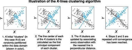
To find ${\widehat{B}}_{\mathit{\text{KU}}}$, we propose the K-lines clustering algorithm, which is inspired by the well-known K-means algorithm (Lloyd 1982). The K-means algorithm cannot account for within-cluster correlation structures but can only identify spherical clusters under a distance metric, for example, the Euclidean distance. In contrast, the K-lines algorithm finds clusters that exhibit strong within-cluster correlations; it is specifically designed for applications where two real-valued variables have distinct correlations in different hidden clusters. We note that the K-lines algorithm is a special case of subspace clustering (Vidal 2010).

As an iterative procedure, the K-lines clustering algorithm includes two alternating steps in each iteration. The recentering step uses the current cluster assignment (i.e., line memberships) to update each cluster line center, which minimizes the within-cluster sum of squared perpendicular distances of data points to the line center. The assignment step updates the cluster assignment based on the current cluster line centers: assign every data point to its closest cluster line center in the perpendicular distance. The two steps alternate until the algorithm converges. Figure 2 illustrates the K-lines clustering algorithm.

Fig. 2 An illustration of the K-lines clustering algorithm.

Algorithm 1:

K-lines clustering algorithm

Initialization: Assign random initial clusters ${\mathcal{C}}_1^{(0)},\dots ,{\mathcal{C}}_K^{(0)}$, such that ${\cup }_{k=1}^K{\mathcal{C}}_k^{(0)}=\{1,\dots ,n\}$.

The algorithm proceeds by alternating between two steps. In the tth iteration, $t=1,2,\dots$

Recentering step: Calculate the cluster line centers ${\widehat{\beta }}_{1U}^{(t)},\dots ,{\widehat{\beta }}_{\mathit{\text{KU}}}^{(t)}$ based on the cluster assignment ${\mathcal{C}}_1^{(t-1)},\dots ,{\mathcal{C}}_K^{(t-1)}$ by (2.6).

Assignment step: Update the cluster assignment for $k=1,\dots ,K$ $${\mathcal{C}}_k^{(t)}=\left\{i:d_{\perp }\left({(X_i,Y_i)}^{\mathsf{T}},{\widehat{\beta }}_{\mathit{\text{kU}}}^{(t)}\right)\le d_{\perp }\left({(X_i,Y_i)}^{\mathsf{T}},{\widehat{\beta }}_{\mathit{\text{sU}}}^{(t)}\right),\text{ for all }s=1,\dots ,K\right\}.$$

Stop the iteration when the cluster assignment no longer changes.

Output: Cluster assignment ${\mathcal{C}}_1,\dots ,{\mathcal{C}}_K$; Sample-level unspecified line centers ${\widehat{\beta }}_{1U},\dots ,{\widehat{\beta }}_{\mathit{\text{KU}}}$.

The recentering step updates each cluster center using the major axis regression, which minimizes the sum of squares of the perpendicular distances from points to the regression line. The major axis regression line is the first principal component of the two variables’ sample covariance matrix (Jolliffe 1982; Smith 2009). Given the cluster assignment in the $(t-1)$th iteration: ${\mathcal{C}}_1^{(t-1)},\dots ,{\mathcal{C}}_K^{(t-1)}$, the updated kth cluster center is (2.6) $$\begin{array}{c}{\widehat{\beta }}_{\mathit{\text{kU}}}^{(t)}=\underset{\beta }{\text{arg} \mathrm{\text{min}}}\sum _{i\in {\mathcal{C}}_k^{(t-1)}}{d}_{\perp }^2\left({(X_i,Y_i)}^{\mathsf{T}},\beta \right)\\ ={\left({\widehat{\theta }}_{\mathit{\text{kU}}},{\widehat{u}}_{12,k}{\overline{X}}_{\mathit{\text{kU}}}-{\widehat{u}}_{11,k}{\overline{Y}}_{\mathit{\text{kU}}}\right)}^{\mathsf{T}},\end{array}$$(2.6) where $\hspace{0.17em}\mathrm{\text{cos}}\hspace{0.17em}{\widehat{\theta }}_{\mathit{\text{kU}}}={\widehat{u}}_{12,k}$, $\hspace{0.17em}\mathrm{\text{sin}}\hspace{0.17em}{\widehat{\theta }}_{\mathit{\text{kU}}}=-{\widehat{u}}_{11,k}$, and ${({\widehat{u}}_{11,k},{\widehat{u}}_{12,k})}^{\mathsf{T}}$ is the first eigenvector of the sample covariance matrix $${\left|{\mathcal{C}}_k^{(t-1)}\right|}^{-1}\left[\begin{array}{cc}\sum _{i\in {\mathcal{C}}_k^{(t-1)}}{(X_i-{\overline{X}}_{\mathit{\text{kU}}})}^2& \sum _{i\in {\mathcal{C}}_k^{(t-1)}}(X_i-{\overline{X}}_{\mathit{\text{kU}}})(Y_i-{\overline{Y}}_{\mathit{\text{kU}}})\\ \sum _{i\in {\mathcal{C}}_k^{(t-1)}}(X_i-{\overline{X}}_{\mathit{\text{kU}}})(Y_i-{\overline{Y}}_{\mathit{\text{kU}}})& \sum _{i\in {\mathcal{C}}_k^{(t-1)}}{(Y_i-{\overline{Y}}_{\mathit{\text{kU}}})}^2\end{array}\right],$$ with ${\overline{X}}_{\mathit{\text{kU}}}=|{\mathcal{C}}_k^{(t-1)}{|}^{-1}\sum _{i\in {\mathcal{C}}_k^{(t-1)}}{X}_i$ and ${\overline{Y}}_{\mathit{\text{kU}}}=|{\mathcal{C}}_k^{(t-1)}{|}^{-1}$ $\sum _{i\in {\mathcal{C}}_k^{(t-1)}}{Y}_i$.

Similar to the K-means clustering algorithm, the K-lines clustering algorithm is not guaranteed to find the global minimizer, $\text{arg} {\mathrm{\text{min}}}_{{\mathrm{B}}_{\mathrm{K}}}\mathrm{W}({\mathrm{B}}_{\mathrm{K}},{\mathrm{P}}_{\mathrm{n}})$. Empirically, we run the K-lines clustering algorithm for M times with random initializations and obtain M multisets of unspecified line centers $B_K^{(1)},\dots ,B_K^{(M)}$. Then we set ${\widehat{B}}_{\mathit{\text{KU}}}\in \text{arg} {\mathrm{\text{min}}}_{{\mathrm{B}}_{\mathrm{K}}\in \{{\mathrm{B}}_{\mathrm{K}}^{(1)},\dots ,{\mathrm{B}}_{\mathrm{K}}^{(\mathrm{M})}\}}\mathrm{W}({\mathrm{B}}_{\mathrm{K}},{\mathrm{P}}_{\mathrm{n}})$. Regarding the effects of M, see Section B.3 in the supplementary material. In the R package gR2, the default setting is M = 30 if $n\ge 50$, and $M=\lfloor 1500/n\rfloor$ if n < 50.

Remark 2.1.

Normalization. Regarding whether $X_1,\dots ,X_n$ and $Y_1,\dots ,Y_n$ should be separately normalized before the K-lines algorithm is applied, the decision is problem-specific and depending on the scales of X and Y, same as for K-means clustering.

Remark 2.2.

Computational complexity. The complexity of the K-lines algorithm is O(nKT), the same as Lloyd’s implementation of the K-means algorithm for a given initialization with T iterations. The reason is that the K-lines algorithm and Loyld’s K-means algorithm have only two differences: (a) calculation of K cluster centers, whose complexity is $O(2^{2}n+2^3)=O(n)$ for finding the first principal components in K-lines versus O(n) for calculating the arithmetic means in K-means; (b) calculation of distances from data points to cluster centers, whose complexity is O(n) in both K-means and K-lines.

Remark 2.3.

Data-driven choice of K. When users do not have prior knowledge about the value of K, how to choose K becomes an important question in practice. Some methods for choosing K in K-means clustering can be adapted. For example, the elbow method, though not theoretically principled, is visually appealing to practitioners and widely used. It employs a scree plot whose horizontal axis displays a range of K values, and whose vertical axis shows the average within-cluster sum of squared distances corresponding to each K. For our K-lines algorithm, it is reasonable to use a scree plot to show how $W(B_K,P_n)$, the average within-cluster squared perpendicular distance defined in (2.4), decreases as K increases.

Alternatively, when it is reasonable to assume that $(X,Y)|(Z=k)$ follows a bivariate Gaussian distribution for all $k=1,\dots ,K$, one may use the Akaike information criterion (AIC) to choose K. Specifically, AIC is defined as (2.7) $$\begin{array}{c}\text{AIC}(K)=2(6K-1)-2\sum _{i=1}^n\hspace{0.17em}\mathrm{\text{log}}\hspace{0.17em}p\left(X_i,Y_i|{\{{\widehat{p}}_{\mathit{\text{kU}}},{\widehat{\mu }}_{\mathit{\text{kU}}},{\widehat{\Sigma }}_{\mathit{\text{kU}}}\}}_{k=1}^K\right)\\ \hspace{1em}=2(6K-1)-{\pi }^{-1}\sum _{i=1}^n\hspace{0.17em}\mathrm{\text{log}}\hspace{0.17em}[\sum _{k=1}^K{\widehat{p}}_{\mathit{\text{kU}}}{\left|{\widehat{\Sigma }}_{\mathit{\text{kU}}}\right|}^{-1/2}\\ \mathrm{\hspace{1em}}\mathrm{\hspace{1em}}\hspace{0.17em}\mathrm{\text{exp}}\hspace{0.17em}\left\{-\frac{1}{2}{\left({(X_i,Y_i)}^{\mathsf{T}}-{\widehat{\mu }}_{\mathit{\text{kU}}}\right)}^{\mathsf{T}}{\widehat{\Sigma }}_{\mathit{\text{kU}}}^{-1}\left({(X_i,Y_i)}^{\mathsf{T}}-{\widehat{\mu }}_{\mathit{\text{kU}}}\right)\right\}],\end{array}$$(2.7) where the first term is $2(6K-1)$ because there are 6 parameters for each component and the component proportions sum to 1; in the second term, ${\widehat{p}}_{\mathit{\text{kU}}}=\left|{\mathcal{C}}_k\right|/n,{\widehat{\mu }}_{\mathit{\text{kU}}}={({\overline{X}}_{\mathit{\text{kU}}},{\overline{Y}}_{\mathit{\text{kU}}})}^{\mathsf{T}}$, $$\begin{array}{c}{\widehat{\Sigma }}_{\mathit{\text{kU}}}=|{\mathcal{C}}_k{|}^{-1}\\ \left[\begin{array}{cc}\sum _{i\in {\mathcal{C}}_k}{(X_i-{\overline{X}}_{\mathit{\text{kU}}})}^2& \sum _{i\in {\mathcal{C}}_k}(X_i-{\overline{X}}_{\mathit{\text{kU}}})(Y_i-{\overline{Y}}_{\mathit{\text{kU}}})\\ \sum _{i\in {\mathcal{C}}_k}(X_i-{\overline{X}}_{\mathit{\text{kU}}})(Y_i-{\overline{Y}}_{\mathit{\text{kU}}})& \sum _{i\in {\mathcal{C}}_k}{(Y_i-{\overline{Y}}_{\mathit{\text{kU}}})}^2\end{array}\right].\end{array}$$

We will demonstrate the elbow method and the AIC method in Section 4.2.

2.2.2 Sample-Level Generalized Pearson Correlation Square (Unspecified)

Powered by the K-lines algorithm, we introduce the sample surrogate indices ${\widehat{Z}}_i\in \{1,\dots ,K\},i=1,\dots ,n$, based on which we then define the sample-level generalized Pearson correlation square for this line-membership unspecified scenario.

Definition 2.4.

Suppose that Algorithm 1 outputs K unspecified line centers ${\widehat{\beta }}_{1U},\dots ,{\widehat{\beta }}_{\mathit{\text{KU}}}$. Also suppose that the probability that (X_i, Y _i) is equally close to more than one line center is zero. For each (X_i, Y _i), we define its sample surrogate index (2.8) $${\widehat{Z}}_i=\underset{k\in \{1,\dots ,K\}}{\text{arg} \mathrm{\text{min}}}{d}_{\perp }\left({(X_i,Y_i)}^{\mathsf{T}},{\widehat{\beta }}_{\mathit{\text{kU}}}\right),i=1,\dots ,n.$$(2.8)

Definition 2.5.

At the sample level, when observations ${\{(X_i,Y_i)\}}_{i=1}^n$ have line memberships unspecified, the generalized Pearson correlation square is defined as (2.9) $$R_{\mathit{\text{GU}}}^2=\sum _{k=1}^K{\widehat{p}}_{\mathit{\text{kU}}}·{\widehat{\rho }}_{\mathit{\text{kU}}}^2,$$(2.9) where G stands for generalized, U stands for unspecified, ${\widehat{p}}_{\mathit{\text{kU}}}=\frac{1}{n}{\sum }_{i=1}^{n}I({\widehat{Z}}_i=k)$, $${\widehat{\rho }}_{\mathit{\text{kU}}}^2=\frac{{\left\{\sum _{i=1}^n\left(X_i-{\overline{X}}_{\mathit{\text{kU}}}\right)\left(Y_i-{\overline{Y}}_{\mathit{\text{kU}}}\right)I({\widehat{Z}}_i=k)\right\}}^2}{\left\{\sum _{i=1}^n{\left(X_i-{\overline{X}}_{\mathit{\text{kU}}}\right)}^{2}I({\widehat{Z}}_i=k)\right\}\left\{\sum _{i=1}^n{\left(Y_i-{\overline{Y}}_{\mathit{\text{kU}}}\right)}^{2}I({\widehat{Z}}_i=k)\right\}},$$ $${\overline{X}}_{\mathit{\text{kU}}}=n_{\mathit{\text{kU}}}^{-1}\sum _{i=1}^n{X}_{i}I({\widehat{Z}}_i=k),{\overline{Y}}_{\mathit{\text{kU}}}=n_{\mathit{\text{kU}}}^{-1}\sum _{i=1}^n{Y}_{i}I({\widehat{Z}}_i=k),\mathit{\text{and }}{n}_{\mathit{\text{kU}}}=\sum _{i=1}^{n}I({\widehat{Z}}_i=k).$$

Remark 2.4.

Besides $R_{\mathit{\text{GU}}}^2$, the cluster-specific Pearson correlation squares ${\widehat{\rho }}_{1U}^2,\dots ,{\widehat{\rho }}_{\mathit{\text{KU}}}^2$ are useful for identifying the clusters (subgroups of data points) that exhibit distinct, strong linear dependences.

2.2.3 Population-Level Generalized Pearson Correlation Square (Unspecified)

Analogous to the definition of sample-level unspecified line centers (Definition 2.3), we define the population-level unspecified line centers as the K lines that minimize the expected squared perpendicular distance of (X, Y) to its closest line.

Definition 2.6.

We define the expected within-cluster squared perpendicular distance as (2.10) $$W(B_K,P)=E\left\{\underset{\beta \in B_K}{\mathrm{\text{min}}}{d}_{\perp }^2\left({(X,Y)}^{\mathsf{T}},\beta \right)\right\},$$(2.10) where P is the joint probability measure of (X, Y). Then we define a multiset of population-level unspecified line centers, $B_{\mathit{\text{KU}}}=\{{\beta }_{1U},\dots ,{\beta }_{\mathit{\text{KU}}}\}$, where ${\beta }_{\mathit{\text{kU}}}={({\theta }_{\mathit{\text{kU}}},c_{\mathit{\text{kU}}})}^{\mathsf{T}}$ is the kth line center, as (2.11) $$B_{\mathit{\text{KU}}}\in \underset{B_K}{\text{arg} \mathrm{\text{min}}}W(B_K,P),$$(2.11) where the subindex U stands for unspecified.

Provided that B_KU is uniquely determined, we define a random surrogate index $\tilde{Z}\in \{1,\dots ,K\}$ as the index of the line center to which (X, Y) is closest.

Definition 2.7.

Suppose that the unspecified line centers ${\beta }_{1U},\dots ,{\beta }_{\mathit{\text{KU}}}$ at the population level are unique. Also, suppose that the probability that (X, Y) is equally close to multiple line centers is zero. We define a random surrogate index as (2.12) $$\tilde{Z}=\underset{k\in \{1,\dots ,K\}}{\text{arg} \mathrm{\text{min}}}{d}_{\perp }\left({(X,Y)}^{\mathsf{T}},{\beta }_{\mathit{\text{kU}}}\right).$$(2.12)

Motivated by ${\rho }_{\mathit{\text{GS}}}^2$, we define the population-level generalized Pearson correlation square for the line-membership unspecified scenario, based on $(X,Y,\tilde{Z})$.

Definition 2.8.

At the population level, when no line membership variable is specified (the “unspecified scenario”), the generalized Pearson correlation square between X and Y is (2.13) $${\rho }_{\mathit{\text{GU}}}^2=\sum _{k=1}^K{p}_{\mathit{\text{kU}}}{\rho }_{\mathit{\text{kU}}}^2,$$(2.13) where the subindex G stands for generalized, U stands for unspecified, $p_{\mathit{\text{kU}}}=P(\tilde{Z}=k)$, and ${\rho }_{\mathit{\text{kU}}}^2={\text{cov}}^2(X,Y|\tilde{Z}=k)/\{\text{var}(X|\tilde{Z}=k)\text{var}(Y|\tilde{Z}=k)\}$.

Remark 2.5.

Relations and distinctions between the specified and unspecified scenarios.

1. ${\rho }_{\mathit{\text{GU}}}^2\ge {\rho }_{\mathit{\text{GS}}}^2$. The proof is in the supplementary material.

2. $R_{\mathit{\text{GU}}}^2$ is not an estimator of ${\rho }_{\mathit{\text{GS}}}^2$; rather, it is an estimator of ${\rho }_{\mathit{\text{GU}}}^2$. Hence, the consistency of $R_{\mathit{\text{GU}}}^2$ does not rely on a specific distributional assumption, for example, bivariate Gaussian mixture model, just like the R². If the goal were to use $R_{\mathit{\text{GU}}}^2$ as an estimator of ${\rho }_{\mathit{\text{GS}}}^2$, a specific mixture model must be assumed. Then the K-lines algorithm should be replaced by the Expectation-Maximization (EM) algorithm to decide the sample surrogate indices ${\widehat{Z}}_1,\dots ,{\widehat{Z}}_n$. When the EM algorithm converges to the global optimum and returns the maximum-likelihood estimates of mixture model parameters, the corresponding $R_{\mathit{\text{GU}}}^2$ will be an asymptotically unbiased estimator of ${\rho }_{\mathit{\text{GS}}}^2$.

3 Asymptotic Distributions of Sample-Level Generalized Pearson Correlation Squares

To enable statistical inference of the population-level measures ${\rho }_{\mathit{\text{GS}}}^2$ (2.1) and ${\rho }_{\mathit{\text{GU}}}^2$ (2.13), we derive the first-order asymptotics of the sample-level measures $R_{\mathit{\text{GS}}}^2$ (2.2) and $R_{\mathit{\text{GU}}}^2$ (2.9). In the asymptotic results below, we consider all parameters as fixed and only allow the sample size n to go to infinity.

Theorem 3.1.

Under the line-membership specified scenario, we define $$\begin{array}{c}{\mu }_{X^c{Y}^d,\mathit{\text{kS}}}=E\{{\left(\frac{X-E(X|Z=k)}{\text{var}{(X|Z=k)}^{1/2}}\right)}^c\\ \mathrm{\hspace{1em}}\mathrm{\hspace{1em}}\hspace{1em}{\left(\frac{Y-E(Y|Z=k)}{\text{var}{(Y|Z=k)}^{1/2}}\right)}^d|Z=k\},c,d\in N.\end{array}$$

Assume ${\mu }_{X^4,\mathit{\text{kS}}}<\infty$ and ${\mu }_{Y^4,\mathit{\text{kS}}}<\infty$ for all $k=1,\dots ,K$. Then (3.1) $$\sqrt{n}\left(R_{\mathit{\text{GS}}}^2-{\rho }_{\mathit{\text{GS}}}^2\right)\stackrel{d}{\to }N\left(\mathrm{}0,\sum _{k=1}^K\left(A_{\mathit{\text{kS}}}+B_{\mathit{\text{kS}}}\right)+2\underset{1\le k<r\le K}{\sum \sum }{C}_{\mathit{\text{krS}}}\mathrm{}\right),$$(3.1) where $$\begin{array}{c}{A}_{\mathit{\text{kS}}}=p_{\mathit{\text{kS}}}[{\rho }_{\mathit{\text{kS}}}^4\left({\mu }_{X^4,\mathit{\text{kS}}}+2{\mu }_{X^2{Y}^2,\mathit{\text{kS}}}+{\mu }_{Y^4,\mathit{\text{kS}}}\right)\\ -4{\rho }_{\mathit{\text{kS}}}^3\left({\mu }_{X^{3}Y,\mathit{\text{kS}}}+{\mu }_{X{Y}^3,\mathit{\text{kS}}}\right)+4{\rho }_{\mathit{\text{kS}}}^2{\mu }_{X^2{Y}^2,\mathit{\text{kS}}}],\\ B_{\mathit{\text{kS}}}=p_{\mathit{\text{kS}}}\left(1-p_{\mathit{\text{kS}}}\right){\rho }_{\mathit{\text{kS}}}^4,\hspace{1em}\text{and}\hspace{1em}{C}_{\mathit{\text{krS}}}=-p_{\mathit{\text{kS}}} p_{\mathit{\text{rS}}} {\rho }_{\mathit{\text{kS}}}^2 {\rho }_{\mathit{\text{rS}}}^2.\end{array}$$

Note that Theorem 3.1 does not rely on any distributional assumptions. When it is applied to the special case where $(X,Y)|Z$ follows a bivariate Gaussian distribution, we obtain a much simpler form of the first-order asymptotic distribution of $R_{\mathit{\text{GS}}}^2$.

Corollary 3.1.

Under the special case where $(X,Y)|(Z=k)$ follows a bivariate Gaussian distribution for all $k=1,\dots ,K$, the asymptotic variance of $\sqrt{n}(R_{\mathit{\text{GS}}}^2-{\rho }_{\mathit{\text{GS}}}^2)$ in Theorem 3.1 is simplified and becomes (3.2) $$\sum _{k=1}^K\left[4 p_{\mathit{\text{kS}}} {\rho }_{\mathit{\text{kS}}}^2{\left(1-{\rho }_{\mathit{\text{kS}}}^2\right)}^2+p_{\mathit{\text{kS}}}\left(1-p_{\mathit{\text{kS}}}\right){\rho }_{\mathit{\text{kS}}}^4\right]$$(3.2) (3.3) $$\hspace{1em}-2\underset{1\le k<r\le K}{\sum \sum }{p}_{\mathit{\text{kS}}} p_{\mathit{\text{rS}}} {\rho }_{\mathit{\text{kS}}}^2 {\rho }_{\mathit{\text{rS}}}^2,$$(3.3) which only depends on p_kS and ${\rho }_{\mathit{\text{kS}}}^2,k=1,\dots ,K$.

To derive an analog of Theorem 3.1 and Corollary 3.1 for the unspecified scenario, we need to show that each sample surrogate index ${\widehat{Z}}_i,i=1,\dots ,n$, converges in distribution to the random surrogate index $\tilde{Z}$. A sufficient condition is the strong consistency of the K sample-level unspecified line centers ${\widehat{B}}_{\mathit{\text{KU}}}=\{{\widehat{\beta }}_{1U},\dots ,{\widehat{\beta }}_{\mathit{\text{KU}}}\}$ to the K population-level unspecified line centers $B_{\mathit{\text{KU}}}=\{{\beta }_{1U},\dots ,{\beta }_{\mathit{\text{KU}}}\}$.

Theorem 3.2.

Suppose that $\int {\Vert {(x,y)}^{\mathsf{T}}\Vert }^{2}P({(\mathit{\text{dx}},\mathit{\text{dy}})}^{\mathsf{T}})<\infty$ and that for each $k=1,\dots ,K$ there is a unique multiset $B_{\mathit{\text{kU}}}=\text{arg} {\mathrm{\text{min}}}_{{\mathrm{B}}_{\mathrm{k}}}\mathrm{W}({\mathrm{B}}_{\mathrm{k}},\mathrm{P})$. Also assume that the globally optimal sample-level unspecified line centers ${\widehat{B}}_{\mathit{\text{KU}}}=\text{arg} {\mathrm{\text{min}}}_{{\mathrm{B}}_{\mathrm{K}}}\mathrm{W}({\mathrm{B}}_{\mathrm{K}},{\mathrm{P}}_{\mathrm{n}})$ is attained and unique. Then as $n\to \infty ,{\widehat{B}}_{\mathit{\text{KU}}}\to B_{\mathit{\text{KU}}}$ and $W({\widehat{B}}_{\mathit{\text{KU}}},P_n)\to W(B_{\mathit{\text{KU}}},P)$ almost surely.

The first statement of Theorem 3.2 means that there exists an ordering of the elements in ${\widehat{B}}_{\mathit{\text{KU}}}=\{{\widehat{\beta }}_{1U},\dots ,{\widehat{\beta }}_{\mathit{\text{KU}}}\}$ and $B_{\mathit{\text{KU}}}=\left\{{\beta }_{1U},\dots ,{\beta }_{\mathit{\text{KU}}}\right\}$ such that as the sample size $n\to \infty$, $${\widehat{\beta }}_{\mathit{\text{kU}}}\to {\beta }_{\mathit{\text{kU}}}\text{ almost surely},k=1,\dots ,K.$$

Based on Theorems 3.1 and 3.2, we derive the asymptotic distribution of $R_{\mathit{\text{GU}}}^2$.

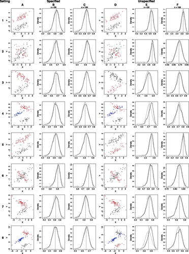
Fig. 3 Comparison of the asymptotic distributions and the finite-sample distributions of $R_{\mathit{\text{GS}}}^2$ and $R_{\mathit{\text{GU}}}^2$. A: Example samples with n = 100; colors and symbols represent values of Z. B–C: Finite-sample distributions n = 50 or 100 (black solid curves) versus the asymptotic distribution (black dotted curves) of $R_{\mathit{\text{GS}}}^2$; the vertical dashed lines mark the values of ${\rho }_{\mathit{\text{GS}}}^2$. D: Example samples with n = 100; colors and symbols represent values of $\tilde{Z}$ inferred by the K-lines algorithm. E–F: Finite-sample distributions of n = 50 or 100 (black solid curves) versus the asymptotic distribution (black dotted curves) of $R_{\mathit{\text{GU}}}^2$; the vertical dashed lines mark the values of ${\rho }_{\mathit{\text{GU}}}^2$.

Theorem 3.3.

Under the line-membership unspecified scenario, we define $$\begin{array}{c}{\mu }_{X^c{Y}^d,\mathit{\text{kU}}}=E\{{\left(\frac{X-E\left[X\right|\tilde{Z}=k]}{\text{var}{(X|\tilde{Z}=k)}^{1/2}}\right)}^c\\ \mathrm{\hspace{1em}}\mathrm{\hspace{1em}}\hspace{1em}{\left(\frac{Y-E\left[Y\right|\tilde{Z}=k]}{\text{var}{(Y|\tilde{Z}=k)}^{1/2}}\right)}^d|\tilde{Z}=k\},c,d\in N,\end{array}$$where $\tilde{Z}$ is the random surrogate index defined in (2.12). Assume ${\mu }_{X^4,\mathit{\text{kU}}}<\infty$ and ${\mu }_{Y^4,\mathit{\text{kU}}}<\infty$ for all $k=1,\dots ,K$. Then (3.4) $$\begin{array}{c}\sqrt{n}\left(R_{\mathit{\text{GU}}}^2-{\rho }_{\mathit{\text{GU}}}^2\right)\\ \stackrel{d}{\to }N\left(0,\sum _{k=1}^K\left(A_{\mathit{\text{kU}}}+B_{\mathit{\text{kU}}}\right)+2\underset{1\le k<r\le K}{\sum \sum }{C}_{\mathit{\text{krU}}}\right)\text{ ,}\end{array}$$(3.4) where $$\begin{array}{c}{A}_{\mathit{\text{kU}}}=p_{\mathit{\text{kU}}}[{\rho }_{\mathit{\text{kU}}}^4\left({\mu }_{X^4,\mathit{\text{kU}}}+2{\mu }_{X^2{Y}^2,\mathit{\text{kU}}}+{\mu }_{Y^4,\mathit{\text{kU}}}\right)\\ \mathrm{\hspace{1em}}\mathrm{\hspace{1em}}-4{\rho }_{\mathit{\text{kU}}}^3\left({\mu }_{X^{3}Y,\mathit{\text{kU}}}+{\mu }_{X{Y}^3,\mathit{\text{kU}}}\right)+4{\rho }_{\mathit{\text{kU}}}^2{\mu }_{X^2{Y}^2,\mathit{\text{kU}}}],\\ B_{\mathit{\text{kU}}}=p_{\mathit{\text{kU}}}\left(1-p_{\mathit{\text{kU}}}\right){\rho }_{\mathit{\text{kU}}}^4,\hspace{1em}\text{and}\hspace{1em}{C}_{\mathit{\text{krU}}}=-p_{\mathit{\text{kU}}} p_{\mathit{\text{rU}}} {\rho }_{\mathit{\text{kU}}}^2 {\rho }_{\mathit{\text{rU}}}^2.\end{array}$$

Corollary A.1 presents a simpler form of Theorem 3.3 under an unrealistic assumption that $(X,Y)|\tilde{Z}$ follows a bivariate Gaussian distribution. Despite being unrealistic, this simpler form empirically works well in numerical simulations (Section 4.1).

Remark 3.1.

When K = 1, the asymptotic distributions of $R_{\mathit{\text{GS}}}^2$ and $R_{\mathit{\text{GU}}}^2$ in Theorems 3.1 and 3.3 both reduce to the asymptotic distribution of R². In the special case that K = 1 and (X, Y) follows bivariate Gaussian distribution with correlation ρ, the asymptotic distribution of $R_{\mathit{\text{GS}}}^2$ in Corollary 3.1 reduces to $\sqrt{n}(R^2-{\rho }^2)\stackrel{d}{\to }N(0,4{\rho }^2{(1-{\rho }^2)}^2)$.

Proofs are in the supplementary material. In Section 4.1, we will numerically show that the asymptotic distribution in Theorem 3.3 works well when K is chosen by the AIC.

4 Numerical Simulations

In this section, we perform simulation studies to numerically verify the theoretical results in Section 3 and to compare our generalized Pearson correlation squares with multiple existing association measures in terms of statistical power. We also demonstrate the effectiveness of our proposed approaches for choosing K, the number of line components in the line-membership unspecified scenario.

4.1 Numerical Verification of Theoretical Results

We first compare the asymptotic distributions in Section 3 with numerically simulated finite-sample distributions under 8 settings (Table 1), where $(X,Y)|Z$ follows a bivariate Gaussian distribution under the first 4 settings and a bivariate t distribution under the latter 4 settings. Under each setting, we generate B = 1000 samples with sizes n = 50 or 100, calculate $R_{\mathit{\text{GS}}}^2$ and $R_{\mathit{\text{GU}}}^2$ on each sample, and compare the simulated finite-sample distributions of $R_{\mathit{\text{GS}}}^2$ and $R_{\mathit{\text{GU}}}^2$ to the corresponding asymptotic distributions. In the first 4 settings, the asymptotic distributions are from Corollaries 3.1 and A.1 (the bivariate Gaussian results); in the latter 4 settings, the asymptotic distributions are from Theorems 3.1 and 3.3 (the general results). The comparison results (Figure 3) show that the finite-sample distributions and the asymptotic results have good agreement, justifying the use of the asymptotic distributions for statistical inference of ${\rho }_{\mathit{\text{GS}}}^2$ or ${\rho }_{\mathit{\text{GU}}}^2$ on a finite sample.

Table 1 Eight settings in simulation studies (Section 4), with each setting indicating a mixture of linear dependences.

Setting	K	Population	Parameters
1	K = 2		$p_1=p_2=0.5$
			${\mu }_1={(0,-2)}^{\mathsf{T}},{\mu }_2={(0,2)}^{\mathsf{T}}$
			${\Sigma }_1={\Sigma }_2=\left[\begin{array}{cc}1& 0.8\\ 0.8& 1\end{array}\right]$
2	K = 2	Specified:	$p_1=p_2=0.5$
		$P(Z=k)=p_k$	${\mu }_1={\mu }_2={(0,0)}^{\mathsf{T}}$
		$(X,Y)|(Z=k)\sim N({\mu }_k,{\Sigma }_k)$	${\Sigma }_1=\left[\begin{array}{cc}1& 0.8\\ 0.8& 1\end{array}\right],{\Sigma }_2=\left[\begin{array}{cc}1& -0.8\\ -0.8& 1\end{array}\right]$
		$k=1,\dots ,K$
3	K = 2		$p_1=0.3,p_2=0.7$
		Unspecified:	${\mu }_1={(0,-2)}^{\mathsf{T}},{\mu }_2={(0,2)}^{\mathsf{T}}$
		${\sum }_{k=1}^K{p}_k N({\mu }_k,{\Sigma }_k)$	${\Sigma }_1=\left[\begin{array}{cc}1& 0.8\\ 0.8& 1\end{array}\right],{\Sigma }_2=\left[\begin{array}{cc}1& -0.8\\ -0.8& 1\end{array}\right]$
4	K = 3		$p_1=0.25,p_2=0.5,p_3=0.25$
			${\mu }_1={(0,-2)}^{\mathsf{T}},{\mu }_2={(0,6)}^{\mathsf{T}},{\mu }_3={(-2,2)}^{\mathsf{T}}$
			${\Sigma }_1=\left[\begin{array}{cc}1& 0.8\\ 0.8& 1\end{array}\right],{\Sigma }_2=\left[\begin{array}{cc}1& -0.7\\ -0.7& 1\end{array}\right],{\Sigma }_3=\left[\begin{array}{cc}1& 0.9\\ 0.9& 1\end{array}\right]$
5	K = 2		$p_1=p_2=0.5,{\nu }_1={\nu }_2=8$
			${\mu }_1={(0,-2)}^{\mathsf{T}},{\mu }_2={(0,2)}^{\mathsf{T}}$
			${\Sigma }_1={\Sigma }_2=\left[\begin{array}{cc}1& 0.8\\ 0.8& 1\end{array}\right]$
6	K = 2	Specified:	$p_1=p_2=0.5,{\nu }_1={\nu }_2=8$
		$P(Z=k)=p_k$	${\mu }_1={\mu }_2={(0,0)}^{\mathsf{T}}$
		$(X,Y)|(Z=k)\sim t_{{\nu }_k}({\mu }_k,{\Sigma }_k)$	${\Sigma }_1=\left[\begin{array}{cc}1& 0.8\\ 0.8& 1\end{array}\right],{\Sigma }_2=\left[\begin{array}{cc}1& -0.8\\ -0.8& 1\end{array}\right]$
		$k=1,\dots ,K$
7	K = 2		$p_1=0.3,p_2=0.7,{\nu }_1={\nu }_2=8$
		Unspecified:	${\mu }_1={(0,-2)}^{\mathsf{T}},{\mu }_2={(0,2)}^{\mathsf{T}}$
		${\sum }_{k=1}^K{p}_k t_{{\nu }_k}({\mu }_k,{\Sigma }_k)$	${\Sigma }_1=\left[\begin{array}{cc}1& 0.8\\ 0.8& 1\end{array}\right],{\Sigma }_2=\left[\begin{array}{cc}1& -0.8\\ -0.8& 1\end{array}\right]$
8	K = 3		$p_1=0.25,p_2=0.5,p_3=0.25$
			${\nu }_1={\nu }_2={\nu }_3=8$
			${\mu }_1={(0,-2)}^{\mathsf{T}},{\mu }_2={(0,6)}^{\mathsf{T}},{\mu }_3={(-2,2)}^{\mathsf{T}}$
			${\Sigma }_1=\left[\begin{array}{cc}1& 0.8\\ 0.8& 1\end{array}\right],{\Sigma }_2=\left[\begin{array}{cc}1& -0.7\\ -0.7& 1\end{array}\right],{\Sigma }_3=\left[\begin{array}{cc}1& 0.9\\ 0.9& 1\end{array}\right]$

NOTE: In the settings 1–4, $N({\mu }_k,{\Sigma }_k)$ represents a bivariate Gaussian distribution with the mean vector μ_k and the covariance matrix Σ_k. In the settings 5–8, $t_{{\nu }_k}({\mu }_k,{\Sigma }_k)$ represents a bivariate t distribution with the degrees of freedom ν_k, the location vector μ_k and the shape matrix Σ_k.

In practice, K often needs to be found in a data-driven way under the line-membership unspecified scenario. To verify the behavior of $R_{\mathit{\text{GU}}}^2$ when K is chosen by the AIC in (2.7), we conduct another simulation study to compare $R_{\mathit{\text{GU}}}^2$’s finite-sample distributions with the asymptotic distributions. The results (Fig. S1 in the supplementary material) show that when n = 100, finite-sample and asymptotic distributions still agree well.

However, the asymptotic distributions in Section 3 involve unobservable parameters in the asymptotic variance terms. A classical solution is to plug-in estimates of these parameters. Another common inferential approach is to use the bootstrap, which is computationally more intensive, instead of the closed-form asymptotic distributions. Here we numerically verify whether the plug-in approach works reasonably well for statistical inference of ${\rho }_{\mathit{\text{GS}}}^2$ and ${\rho }_{\mathit{\text{GU}}}^2$. Under each of the eight settings, we simulate two samples with sizes n = 50 and 100, respectively. We then use each sample to construct a 95% confidence interval (CI) of ${\rho }_{\mathit{\text{GS}}}^2$ and ${\rho }_{\mathit{\text{GU}}}^2$ as $R_{\mathit{\text{GS}}}^2\pm 1.96\text{se}(R_{\mathit{\text{GS}}}^2)$ and $R_{\mathit{\text{GU}}}^2\pm 1.96\text{se}(R_{\mathit{\text{GU}}}^2)$, respectively. We construct the standard errors $\text{se}(R_{\mathit{\text{GS}}}^2)$ and $\text{se}(R_{\mathit{\text{GU}}}^2)$ in two ways: square roots of (a) the plug-in estimates of the asymptotic variances of $R_{\mathit{\text{GS}}}^2$ and $R_{\mathit{\text{GU}}}^2$, or (b) the bootstrap estimates of $\text{var}(R_{\mathit{\text{GS}}}^2)$ and $\text{var}(R_{\mathit{\text{GU}}}^2)$. We also calculate the true asymptotic variances of $R_{\mathit{\text{GS}}}^2$ and $R_{\mathit{\text{GU}}}^2$ based on true parameter values and use them to construct the theoretical CIs. The results (Figure S2 in the supplementary material) show that the plug-in and bootstrap approaches construct similar CIs on the same sample. When n increases from 50 to 100, the CIs constructed by both approaches agree better with the theoretical CIs.

We also evaluate the coverage probabilities of the 95% CIs constructed by the plug-in approach and compare them with those of the theoretical CIs. Table S3 in the supplementary material summarizes the results. The theoretical CIs have coverage probabilities close to 95% under all the eight settings, providing additional verification of the asymptotic distributions. Overall, the plug-in confidence intervals have good coverage probabilities, which are increasingly closer to 95% as n increases; their coverage probabilities are in general closer to 95% under the first four bivariate Gaussians settings than under the last four bivariate t settings. The reason is that mixtures of bivariate Gaussians are more concentrated on K lines and better allow the K-lines algorithm to find the sample-level unspecified line centers, thus, reducing the unwanted variance due to failed algorithm convergence and making the plug-in variance estimate of $R_{\mathit{\text{GU}}}^2$ more accurate. Comparing the line-membership specified and unspecified scenarios, the plug-in confidence intervals, as expected, have better coverage probabilities under the specified scenario that has less uncertainty. Table S3 also shows that the two plug-in options do not have obvious differences, suggesting that the first plug-in option (“P1”), which uses the asymptotic variances in the special bivariate Gaussian forms (Corollaries 3.1 and A.1), is robust and can be used in practice for its simplicity.

4.2 Use of Scree Plot and AIC to Choose K

Following Section 2.2, here we demonstrate the performance of the scree plot and the AIC in choosing K under the eight simulation settings. For each setting, we simulate a sample of size n = 100 and evaluate $W(B_K,P_n)$ in (2.4) and $\text{AIC}(K)$ in (2.7) on this sample for K ranging from 1 to 10 (Figure S3 in the supplementary material). For all the eight settings, the scree plots and the AIC both suggest the correct K values. Even though Settings 5–8 violate the bivariate Gaussian assumption required by the AIC, the AIC results are still reasonable. In practice, users may use the scree plot together with the AIC to choose K.

4.3 Power Analysis

To confirm that $R_{\mathit{\text{GU}}}^2$ is a powerful measure for capturing mixed linear dependences, we conduct a simulation study to compare $R_{\mathit{\text{GU}}}^2(K=2)$ with six popular association measures or tests: the squared Pearson correlation (R²), the maximal correlation (maxCor) estimated by the alternating conditional expectation algorithm (Breiman and Friedman 1985), the distance correlation (dCor) Székely, Rizzo, and Bakirov 2007; Székely and Rizzo 2009, the maximal information coefficient (MIC) (Reshef et al. 2011), Chatterjee’s rank correlation ξ (xiCor), and the Heller-Heller-Gorfine (HHG) test for independence.³ All these measures⁴ have values in $[0,1]$.⁵ Our simulation procedure follows Simon and Tibshirani (2014), where each relationship between two real-valued random variables X and Y is composed of a marginal distribution of $X\sim N(0,5^2)$, a noiseless pattern (i.e., relationship) between X and Y, and a random error from $N(0,{\sigma }^2)$ added to Y. The null hypothesis is that X and Y are independent, while the alternative hypothesis is specified by the noiseless pattern and σ. Given a sample size n = 30, 50 or 200, we simulate B = 1000 samples from the alternative hypothesis. On each of these alternative samples, we randomly permute the Y observations to create a null sample. Then for each n we calculate the association measures on the B null samples and decide a rejection threshold for each measure as the $(1-\alpha )$ quantile of its B null values, where $\alpha =0.05$ is the significance level. Next, we calculate the association measures on the B alternative samples, compare each measure’s B alternative values to its rejection threshold, and estimate the measure’s power as the proportion of alternative values above the rejection threshold. Figure S4 in the supplementary material illustrates each measure’s empirical distribution across alternative samples at each n and σ; all measures’ variances decrease as n increases.⁶

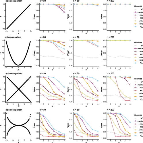
Figure 4 shows that $R_{\mathit{\text{GU}}}^2$ is the most powerful measure when the pattern is a mixture of positive and negative linear dependences. When the pattern is a mixture of nonlinear relationships that can be approximated by a mixture of linear dependences, $R_{\mathit{\text{GU}}}^2$ is still the most powerful. When the pattern is linear, R² is expectedly the most powerful, and the other measures including $R_{\mathit{\text{GU}}}^2$ also have perfect power up to σ = 3 at n = 30. Under a parabola pattern, which can be approximated by two intersecting lines (i.e., the “V” pattern), $R_{\mathit{\text{GU}}}^2$ still has good power and is comparable to xiCor, maxCor, dCor, HHG, and MIC. These results confirm the application potential of $R_{\mathit{\text{GU}}}^2$ in capturing complex relationships that can be approximated by mixtures of linear dependences.

Fig. 4 Power analysis. Simulation studies that compare the statistical power of seven measures/tests: the squared Pearson correlation (R²), the maximal correlation (maxCor), the distance correlation (dCor), the maximal information coefficient (MIC), Chatterjee’s rank correlation (xiCor), the Heller-Heller-Gorfine (HHG) test, and $R_{\mathit{\text{GU}}}^2$ with K = 2. In each row, the noiseless pattern illustrates a relationship between two real-valued random variables X and Y when no noise is added (σ = 0). Under the null hypothesis, X and Y are independent. Varying alternative hypotheses are formed by the noiseless pattern with noise $\sim N(0,{\sigma }^2)$ at varying σ added to Y. Under each alternative hypothesis corresponding to one σ, we estimate the power of the seven measures/tests given each sample size n (columns 2–4).

5 Real Data Applications

5.1 Analysis of the A. thaliana Gene Expression Dataset

Back to our motivating example in A. thaliana, here we use this gene expression dataset (Li et al. 2008) to demonstrate the use of our generalized Pearson correlation squares to capture biologically meaningful gene–gene relationships. The glucosinolate (GSL) biosynthesis pathway has been well studied in A. thaliana, and 31 genes in this pathway have been experimentally identified (Kim et al. 2012). Since genes in the same pathway are functionally related, their relationships should be distinct from their relationships with the other genes outside of the pathway. Hence, a powerful association measure should distinguish the pairwise gene–gene relationships within the GSL pathway from the relationships of randomly paired GSL and non-GSL genes.

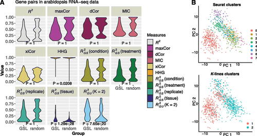
The dataset (Table S4 in the supplementary material) contains n = 232 samples, 26 GSL genes, and four index variables: condition (oxidation, wounding, UV-B light, and drought), treatment (yes and no), replicate (1 and 2), and tissue (root and shoot). We observe that only the tissue variable is a good indicator of linear dependences, as illustrated in Figures 1 and S5–S8 in the supplementary material.

Figure 5(A) shows the values of R², maxCor, dCor, MIC, xiCor, HHG,⁷ and $R_{\mathit{\text{GU}}}^2(K=2)$, all of which do not use index variables, as well as $R_{\mathit{\text{GS}}}^2$, which uses the index variable as condition, treatment, replicate, or tissue. All these measures are computed for the $(\begin{array}{c}26\\ 2\end{array})=325$ GSL gene pairs and 2600 random gene pairs, each of which consists of a GSL gene (out of 26 GSL genes) and a randomly selected non-GSL gene (out of 100 randomly selected non-GSL genes). Among these measures, only $R_{\mathit{\text{GS}}}^2(\text{tissue})$ and $R_{\mathit{\text{GU}}}^2(K=2)$ show significantly stronger relationships (at the significance level of 0.01) within the GSL pathway than in random gene pairs (with respective p-values $1.29\times {10}^{-28}$ and $7.65\times {10}^{-20}$ from one-sided Wilcoxon rank-sum test). Hence, $R_{\mathit{\text{GS}}}^2$ is a useful and powerful measure when a good index variable is available; otherwise, $R_{\mathit{\text{GU}}}^2$ is advantageous in capturing complex but interpretable gene–gene relationships without knowledge of index variables⁸.

Fig. 5 Real data applications of $R_{\mathit{\text{GS}}}^2,R_{\mathit{\text{GU}}}^2$, and the K-lines clustering algorithm. A: Analysis of the Arabidopsis gene expression dataset. We compare 11 measures, including seven unspecified measures (R², maxCor, dCor, MIC, xiCor, HHG, and $R_{\mathit{\text{GU}}}^2$ with K = 2) and four $R_{\mathit{\text{GS}}}^2$ measures with different index variables, in terms of measuring pairwise gene relationships within the GSL pathway (“GSL”) versus relationships between a GSL gene and a randomly paired non-GSL gene (“random”). For each measure, the one-sided Wilcoxon rank-sum test is used to compare the measure’s values in the two groups (“GSL” vs. “random”), and the resulting p-value is marked in each panel. At the significance level of 0.01, $R_{\mathit{\text{GS}}}^2(\text{tissue})$ and $R_{\mathit{\text{GU}}}^2(K=2)$ are the only two measures indicating that the gene pairs within the GSL pathway have significantly stronger relationships than the random GSL-nonGSL gene pairs do. B: Beta cell clusters found by Seurat (left) or the K-lines clustering algorithm (right).

To verify the agreement between the K-lines clusters and the tissue index variable, for every GSL gene pair, we compare the K = 2 sample clusters identified by the K-lines algorithm with the sample groups defined by each of the four index variables (condition, treatment, replicate, and tissue) using Fisher’s exact test⁹ and the adjusted mutual information¹⁰. The results in Table 2 confirm that the K-lines clusters exhibit higher consistency with the tissue variable compared to the other three index variables across the 325 GSL gene pairs, suggesting that the K-lines algorithm separates the samples in good accordance with their tissue types.

Table 2 Comparison of the K-lines clusters and the four index variables (condition, treatment, replicate, and tissue) in the A. thaliana gene expression dataset.

	Fisher’s exact test p-value			Adjusted mutual information
	$<0.05$	$<0.005$	$<0.0005$	Mean	3rd quartile	Max
condition	29.54%	19.69%	11.08%	0.007	0.010	0.090
treatment	34.15%	22.46%	14.77%	0.013	0.019	0.152
replicate	1.85%	0.00%	0.00%	−0.001	0.000	0.019
tissue	72.00%	63.38%	58.77%	0.293	0.578	1.000

NOTE: In columns 1–3, each percentage represents the percentage of the 325 GSL gene pairs whose K-lines clusters have a significant p-value (given a threshold) when compared with an index variable by Fisher’s exact test. In columns 4–6, the mean, 3rd quartile, and maximum of the adjusted mutual information values are reported for the 325 GSL gene pairs whose K-lines clusters are compared with each index variable.

5.2 Identification of Beta Cell Subtypes by K-Lines Clustering

The second example is from a single-cell gene expression dataset of mouse pancreas (Baron et al. 2016). A previous study found that using projective nonnegative matrix factorization (PNMF) to project cells from a high-dimensional (7838) gene expression space to a low-dimensional space of PNMF factors, some PNMF factors exhibited heterogeneous linear relationships with the cell library size (i.e., the total number of sequencing reads mapped to each cell), and each relationship corresponded to a known cell type (Song et al. 2021). Motivated by this finding, here we apply the K-lines clustering algorithm to n = 894 beta cells’ PNMF factors and library sizes. For each of 10 PNMF factors, we pair it up with the cell library size and apply the K-lines clustering algorithm,¹¹ which finds a notable K = 2 pattern (by AIC) for PNMF factor 4 versus cell library size (Figure S9A). Comparing the resulting two beta cell clusters to the default clustering results by the most popular pipeline Seurat using PCA and UMAP visualization, we find that the default Seurat leads to eight clusters including many hardly separable ones, while the two K-lines clusters are distinct in both PCA and UMAP visualization (Figures 5(B) and S9B).

We verify the two K-lines clusters by conducting literature review and performing KEGG pathway enrichment analysis. First, based on the review by Miranda, Macias-Velasco, and Lawson (2021), we map the clusters 1 and 2 to the immature and mature beta subtypes respectively by verifying that mature cell marker genes Gck, Ins1, and Iapp are significantly more highly expressed in cluster 2 than cluster 1 (with one-sided Wilcoxon rank-sum test p-values 0.001001, $<2.2\times {10}^{-16}$, and $<2.2\times {10}^{-16}$, respectively). Second, we confirm this mapping result by using (a) the FindMarkers() function in Seurat to find clusters 1 and 2’s respective marker genes and (b) the R package clusterProfiler 4.0 to find the enriched KEGG pathways within each cluster’s marker genes (Tables S5–S6 in the supplementary material). The results suggest that beta cell cluster 1 is related to the insulin resistance, while cluster 2 is related to the insulin signaling pathway, consistent with previous findings that immature beta cells are over-represented in insulin resistant patients and mature beta cells are responsible for regular insulin secretion, respectively (Miranda, Macias-Velasco, and Lawson 2021).

6 Discussion

The generalized Pearson correlation squares extend the classic and popular Pearson correlation to capturing heterogeneous linear relationships. This new suite of measures has broad potential use in scientific applications. In addition to gene expression analysis, statistical genetics is a potential application domain because genetic variants could exhibit heterogeneous effects on a phenotype. When known subpopulations, for example, race, gender, and geography, cannot explain heterogenous associations between a genetic variant and a phenotype, $R_{\mathit{\text{GU}}}^2$ and the K-lines algorithm could be useful.

A future direction is to extend the generalized Pearson correlation squares to be rank-based. This extension will make the measures robust to outliers and capable of capturing a mixture of monotone relationships.

Another future direction is to generalize the K-lines clustering algorithm to the K-hyperplanes clustering algorithm, following the subspace clustering literature (Vidal 2010). Specifically, for $p\ge 2$ variables, the kth cluster center becomes the $(p-1)$-dimensional hyperplane defined by the top $(p-1)$ principal components of the data points (p-dimensional vectors) assigned to the kth cluster, $k=1,\dots ,K$. In this generalization, we only need to generalize the recentering step in the K-lines clustering algorithm (Algorithm 1) while keeping the assignment step as assigning every data point to the closest hyperplane based on the perpendicular distance. Then, we can generalize a multivariate dependence measure by calculating the weighted sum of the measure’s values across the K clusters.

Supplementary Materials

The online supplementary materials (Supplements.zip) contain 1. the Author Contributions Checklist form (acc_form.pdf); 2. the Supplementary Material file (supplementary_material.pdf) containing proofs of theorems, convergence properties of the K-lines algorithm, more simulation results, another real data application about the dependence of glioma patient survival on CD44 expression, real data description, more tables and figures, and additional references; 3. the reproducibility_materials.zip file including (1) a README.md file, (2) an Rmd file to reproduce the results and the html file knitted from the Rmd file, (3) a data folder containing the datasets and data_description.txt, (4) a results folder containing the intermediate results, (5) a code folder containing R code used in the Rmd file, and (6) the pdf files of Figure S9A and Figure S9B.

Disclosure Statement

The authors report there are no competing interests to declare.

Additional information

Funding

The authors gratefully acknowledge NSF DBI-1846216 and DMS-2113754, NIH/NIGMS R01GM120507 and R35GM140888, Johnson and Johnson WiSTEM2D Award, Sloan Research Fellowship, and UCLA David Geffen School of Medicine W.M. Keck Foundation Junior Faculty Award.

Notes

1 Monotone relationships becomes linear after values of each variable are transformed into ranks.

2 Note that a linear model with group-specific slopes and intercepts (groups specified by the index variable Z) does not provide a desirable measure under the specified scenario. The reason is that the exchangeability is not satisfied: the linear model R² would be different if we swap the two variables X and Y; that is, the two linear models (written in R commands) lm(Y ˜ Z + X:Z) and lm(X ˜ Z + Y:Z) do not give the same R².

3 For the implementation of these measures, see Table S2 in the supplementary material.

4 The HHG test statistic is not an association measure, so ($1-$ HHG test p-value) is used as a measure.

5 Note that xiCor may take negative values at the sample level.

6 The HHG test is not included because ($1-$ HHG test p-value) is too close to 1 most of the time.

7 The HHG test statistic is not an association measure, so ($1-$ HHG test p-value) is used as a measure.

8 In this application, the two variables X and Y refer to two genes with comparable expression levels, so no normalization is performed before K-lines clustering.

9 A smaller p-value more strongly rejects the null hypothesis that the K-lines clusters are independent of an index variable.

10 A larger adjusted mutual information indicates a better agreement between the K-lines clusters and an index variable.

11 In this application, the two variables X and Y refer to the cell library size and a PNMF factor, whose values are on the same scale, so no normalization is performed before K-lines clustering.

References

- Baron, M., Veres, A., Wolock, S. L., Faust, A. L., Gaujoux, R., Vetere, A., Ryu, J. H., Wagner, B. K., Shen-Orr, S. S., Klein, A. M. et al. (2016), “A Single-Cell Transcriptomic Map of the Human and Mouse Pancreas Reveals Inter-and Intra-cell Population Structure,” Cell Systems, 3, 346–360. DOI: 10.1016/j.cels.2016.08.011.
- Benaglia, T., Chauveau, D., Hunter, D., and Young, D. (2009), “mixtools: An r Package for Analyzing Finite Mixture Models,” Journal of Statistical Software, 32, 1–29. DOI: 10.18637/jss.v032.i06.
- Bjerve, S., and Doksum, K. (1993), “Correlation Curves: Measures of Association as Functions of Covariate Values,” The Annals of Statistics, 21, 890–902. DOI: 10.1214/aos/1176349156.
- Breiman, L., and Friedman, J. H. (1985), “Estimating Optimal Transformations for Multiple Regression and Correlation,” Journal of the American Statistical Association, 80, 580–598. DOI: 10.1080/01621459.1985.10478157.
- Chatterjee, S. (2021), “A New Coefficient of Correlation,” Journal of the American Statistical Association, 116, 2009–2022. DOI: 10.1080/01621459.2020.1758115.
- De Veaux, R. D. (1989), “Mixtures of Linear Regressions,” Computational Statistics & Data Analysis, 8, 227–245. DOI: 10.1016/0167-9473(89)90043-1.
- Delicado, P., and Smrekar, M. (2009), “Measuring Non-linear Dependence for Two Random Variables Distributed Along a Curve,” Statistics and Computing, 19, 255–269. DOI: 10.1007/s11222-008-9090-y.
- Gretton, A., Bousquet, O., Smola, A., and Schölkopf, B. (2005), “Measuring Statistical Dependence with Hilbert-Schmidt Norms,” in International Conference on Algorithmic Learning Theory, pp. 63–77, Springer.
- Hawkins, D. S., Allen, D. M., and Stromberg, A. J. (2001), “Determining the Number of Components in Mixtures of Linear Models,” Computational Statistics & Data Analysis, 38, 15–48. DOI: 10.1016/S0167-9473(01)00017-2.
- Heller, R., Heller, Y., and Gorfine, M. (2012), “A Consistent Multivariate Test of Association based on Ranks of Distances,” Biometrika, 100, 503–510. DOI: 10.1093/biomet/ass070.
- Hurn, M., Justel, A., and Robert, C. P. (2003), “Estimating Mixtures of Regressions,” Journal of Computational and Graphical Statistics, 12, 55–79. DOI: 10.1198/1061860031329.
- Jacobs, R. A., Jordan, M. I., Nowlan, S. J., and Hinton, G. E. (1991), “Adaptive Mixtures of Local Experts,” Neural Computation, 3, 79–87. DOI: 10.1162/neco.1991.3.1.79.
- Jolliffe, I. T. (1982), “A Note on the Use of Principal Components in Regression,” Applied Statistics, 31, 300–303. DOI: 10.2307/2348005.
- Jones, P., and McLachlan, G. (1992), “Fitting Finite Mixture Models in a Regression Context,” Australian & New Zealand Journal of Statistics, 34, 233–240.
- Kim, K., Jiang, K., Teng, S. L., Feldman, L. J., and Huang, H. (2012), “Using Biologically Interrelated Experiments to Identify Pathway Genes in Arabidopsis,” Bioinformatics, 28, 815–822. DOI: 10.1093/bioinformatics/bts038.
- Lee, D., and Zhu, B. (2021), “A Semiparametric Kernel Independence Test with Application to Mutational Signatures,” Journal of the American Statistical Association, 116, 1648–1661. DOI: 10.1080/01621459.2020.1871357.
- Leisch, F. (2008), “Modelling Background Noise in Finite Mixtures of Generalized Linear Regression Models,” in COMPSTAT 2008, pp. 385–396, Springer.
- Li, J., Hansen, B. G., Ober, J. A., Kliebenstein, D. J., and Halkier, B. A. (2008), “Subclade of Flavin-Monooxygenases Involved in Aliphatic Glucosinolate Biosynthesis,” Plant Physiology, 148, 1721–1733. DOI: 10.1104/pp.108.125757.
- Li, K.-C. (2002), “Genome-Wide Coexpression Dynamics: Theory and Application,” Proceedings of the National Academy of Sciences, 99, 16875–16880. DOI: 10.1073/pnas.252466999.
- Lloyd, S. (1982), “Least Squares Quantization in PCM,” IEEE Transactions on Information Theory, 28, 129–137. DOI: 10.1109/TIT.1982.1056489.
- Miranda, M. A., Macias-Velasco, J. F., and Lawson, H. A. (2021), “Pancreatic β-cell Heterogeneity in Health and Diabetes: Classes, Sources, and Subtypes,” American Journal of Physiology-Endocrinology and Metabolism, 320, E716–E731. DOI: 10.1152/ajpendo.00649.2020.
- Murtaph, F., and Raftery, A. (1984), “Fitting Straight Lines to Point Patterns,” Pattern Recognition, 17, 479–483. DOI: 10.1016/0031-3203(84)90045-1.
- Quandt, R. E., and Ramsey, J. B. (1978), “Estimating Mixtures of Normal Distributions and Switching Regressions,” Journal of the American Statistical Association, 73, 730–738. DOI: 10.1080/01621459.1978.10480085.
- Reshef, D. N., Reshef, Y. A., Finucane, H. K., Grossman, S. R., McVean, G., Turnbaugh, P. J., Lander, E. S., Mitzenmacher, M., and Sabeti, P. C. (2011), “Detecting Novel Associations in Large Data Sets,” Science, 334, 1518–1524. DOI: 10.1126/science.1205438.
- Scharl, T., Grün, B., and Leisch, F. (2009), “Mixtures of Regression Models for Time Course Gene Expression Data: Evaluation of Initialization and Random Effects,” Bioinformatics, 26, 370–377. DOI: 10.1093/bioinformatics/btp686.
- Shen, C., Priebe, C. E., and Vogelstein, J. T. (2019), “From Distance Correlation to Multiscale Graph Correlation,” Journal of the American Statistical Association, 115, 280–291. DOI: 10.1080/01621459.2018.1543125.
- Simon, N., and Tibshirani, R. (2014), Comment on “Detecting Novel Associations in Large Data Sets” by Reshef et al, Science Dec 16, 2011,” arXiv preprint arXiv:1401.7645.
- Smith, R. J. (2009), “Use and Misuse of the Reduced Major Axis for Line-Fitting,” American Journal of Physical Anthropology: The Official Publication of the American Association of Physical Anthropologists, 140, 476–486. DOI: 10.1002/ajpa.21090.
- Song, D., Li, K., Hemminger, Z., Wollman, R., and Li, J. J. (2021), “scPNMF: Sparse Gene Encoding of Single Cells to Facilitate Gene Selection for Targeted Gene Profiling,” Bioinformatics, 37, i358–i366. DOI: 10.1093/bioinformatics/btab273.
- Székely, G. J., Rizzo, M. L., and Bakirov, N. K. (2007), “Measuring and Testing Dependence by Correlation of Distances,” The Annals of Statistics, 35, 2769–2794. DOI: 10.1214/009053607000000505.
- Székely, G. J., and Rizzo, M. L. (2009), “Brownian Distance Covariance,” The Annals of Applied Statistics, 3, 1236–1265. DOI: 10.1214/09-AOAS312.
- Turner, T. R. (2000), “Estimating the Propagation Rate of a Viral Infection of Potato Plants via Mixtures of Regressions,” Journal of the Royal Statistical Society, Series C, 49, 371–384. DOI: 10.1111/1467-9876.00198.
- Vidal, R. (2010), “A Tutorial on Subspace Clustering,” https://api.semanticscholar.org/CorpusID:7099537
- Wang, X., Jiang, B., and Liu, J. S. (2017), “Generalized R-squared for Detecting Dependence,” Biometrika, 104, 129–139. DOI: 10.1093/biomet/asw071.
- Wang, Y. R., Waterman, M. S., and Huang, H. (2014), “Gene Coexpression Measures in Large Heterogeneous Samples Using Count Statistics,” Proceedings of the National Academy of Sciences, 111, 16371–16376. DOI: 10.1073/pnas.1417128111.
- Wedel, M., and DeSarbo, W. S. (1994), “A Review of Recent Developments in Latent Class Regression Models,” in Advanced Methods of Marketing Research, ed. R.P. Bagozzi, pp. 352–388, Cambridge: Blackwell Publishers.
- Zheng, S., Shi, N.-Z., and Zhang, Z. (2012), “Generalized Measures of Correlation for Asymmetry, Nonlinearity, and Beyond,” Journal of the American Statistical Association, 107, 1239–1252. DOI: 10.1080/01621459.2012.710509.