Sparse Independent Component Analysis with an Application to Cortical Surface fMRI Data in Autism

Abstract

Independent component analysis (ICA) is widely used to estimate spatial resting-state networks and their time courses in neuroimaging studies. It is thought that independent components correspond to sparse patterns of co-activating brain locations. Previous approaches for introducing sparsity to ICA replace the non-smooth objective function with smooth approximations, resulting in components that do not achieve exact zeros. We propose a novel Sparse ICA method that enables sparse estimation of independent source components by solving a non-smooth non-convex optimization problem via the relax-and-split framework. The proposed Sparse ICA method balances statistical independence and sparsity simultaneously and is computationally fast. In simulations, we demonstrate improved estimation accuracy of both source signals and signal time courses compared to existing approaches. We apply our Sparse ICA to cortical surface resting-state fMRI in school-aged autistic children. Our analysis reveals differences in brain activity between certain regions in autistic children compared to children without autism. Sparse ICA selects coactivating locations, which we argue is more interpretable than dense components from popular approaches. Sparse ICA is fast and easy to apply to big data. Supplementary materials for this article are available online, including a standardized description of the materials available for reproducing the work.

KEYWORDS:

• ASD
• Functional connectivity
• ICA
• Neuroimaging
• Sparsity

1 Introduction

Autism spectrum disorder (ASD) is a developmental disorder associated with challenges in social interaction, communication, and repetitive behaviors. ASD is believed to be associated with altered communication between brain regions (Di Martino, Al, and Milham, 2013). Functional connectivity characterizes the co-activation of brain regions (Yeo et al., 2011). To identify areas of the brain that tend to co-activate, independent component analysis (ICA) is commonly applied to resting-state functional magnetic resonance imaging (fMRI) data (Damoiseaux et al., 2006). The independent components (ICs) are known as “resting-state networks,” and the correlations between the time courses of the components reveal brain communication patterns. It is believed that the components should be sparse since most areas of the brain are not part of any given component (Daubechies et al., 2009). However, current approaches usually estimate dense components. The components are typically thresholded in graphical summaries to eliminate inactive locations, while the time courses used in downstream analyses correspond to the original non-sparse components (Erhardt et al., 2011). The thresholded maps are used to aid the interpretation of brain communication patterns, but directly estimating sparse components and their time courses may better reveal the underlying patterns of brain activity.

Our motivating data contain resting-state fMRI measurements from school-age children in the Autism Brain Imaging Exchange (ABIDE) (Di Martino, Al, and Milham, 2013; Di Martino et al., 2017). Our overall scientific goal is to estimate functional connectivity differences between autistic children and children without autism in which functional connectivity is defined by correlations between independent component time courses. The use of ICA to study functional connectivity in autistic children has gained favor in recent years because the standard brain atlases based on adults are not ideal for developmental cohorts. The estimated spatial components play the role of a study-specific brain parcellation (Lombardo et al., 2019; Lidstone et al., 2021; Nebel et al., 2022). Correlations or partial correlations between the time courses of components are analyzed in downstream analyses (Smith et al., 2015).

Fast ICA and Infomax ICA are two of the most popular ICA algorithms (Bell and Sejnowski, 1995; Hyvarinen, 1999). These approaches easily scale to large fMRI datasets and have been popularized in the Group ICA of fMRI Toolbox (GIFT) (Calhoun et al., 2001) and Melodic software (Smith et al., 2004). Although other ICA algorithms exist, neuroimaging studies commonly use either Infomax ICA via GIFT (Lidstone et al., 2021; Nebel et al., 2022) or Fast ICA in Melodic (Smith et al., 2015; Lombardo et al., 2019). However, these popular methods do not produce sparse components, so post-estimation thresholding is typically used for interpretation. As an alternative to thresholding, Melodic includes a post-ICA option that fits a bivariate mixture of Gaussians to Fast ICA components, but the time courses are unchanged. In general, bivariate mixture modeling in ICA is challenging, as its complexity grows exponentially with the number of components. Directly estimating sparse components may improve accuracy and decrease computational costs.

Sparse methods exist in the literature, but they do not estimate simultaneously sparse and independent components. We define a component as sparse if it has a large proportion of elements that are exactly equal to zero. In compressed sensing, sparse dictionary learning estimates a sparse or nearly sparse basis that can reduce noise and achieve data compression (Lee et al., 2006). However, sparse dictionary learning can lead to multiple representations of the same signal, which creates interpretation issues in fMRI. Sparsity has been incorporated into principal component analysis (PCA) through penalized reconstruction error or singular value decomposition (Zou, Hastie, and Tibshirani, 2006; Shen and Huang, 2008; Erichson et al., 2020). Neither sparse dictionary learning nor sparse PCA methods enforce independence among components. Early work on sparse ICA approximates sparse sources by applying a clustering algorithm to principal components (Babaie-Zadeh, Jutten, and Mansour, 2006), but is not scalable to fMRI data. Sparse Fast ICA (Ge et al., 2016) adds a second stage to the Fast ICA algorithm to constrain the source sparsity through a smooth approximation to the l₀ norm, and involves several tuning parameters. Sparse ICA entropy-bound minimization (SICA-EBM) (Boukouvalas et al., 2018; Long et al., 2019) strives to combine sparse dictionary learning with the independence in ICA by incorporating a smooth approximation to l₁ regularization with two tuning parameters. However, it is unclear how to choose the best values and the method is computationally costly. Neither Sparse Fast ICA nor SICA-EBM achieves exact sparsity due to their reliance on smooth approximations. Recently, Lukemire, Pagnoni, and Guo (2023) developed Sparse Bayes ICA, which uses horseshoe priors to select sparse covariate effects in ICA, and thus has a different goal than our present work.

In summary, there are three main challenges in estimating sparse independent components. First, existing ICA methods, including Sparse Fast ICA and SICA-EBM, are only capable of handling smooth objective functions, which limits their ability to impose exact sparsity. Second, ICA optimization involves an orthogonality constraint leading to non-convex optimization, which subsequently necessitates the use of specialized algorithms and may lead to problems with local minima. Thirdly, in fMRI data analysis, the input data is often high-dimensional. An ICA method should be computationally feasible when applied to millions of data points.

In this article, we introduce a novel Sparse Independent Component Analysis (Sparse ICA) method that can be used for both subject and group-level fMRI data analysis. The method achieves precise sparsity by employing the Laplace density and ensures computational efficiency through the relax-and-split framework (Zheng and Aravkin, 2020). A tuning parameter is used to control sparsity, which is selected using a BIC-like criterion. In numerical experiments, our proposed Sparse ICA outperforms existing methods in terms of the accuracy of estimating source signals and time courses, and is computationally efficient. When applied to fMRI data from autistic children, Sparse ICA extracts sparse components that correspond to resting-state networks, and we discover functional connectivity differences between autistic and typically developing children.

The rest of this article is structured as follows. In Section 2, we present the Sparse ICA model from an optimization perspective and introduce the relax-and-split framework for model estimation. We extend Sparse ICA to perform group-level analysis and introduce the BIC criterion for selecting the tuning parameter. In Section 3, we conduct simulation studies to compare the performance of the proposed Sparse ICA with existing ICA approaches. In Section 4, we apply our Sparse ICA method to cortical surface fMRI data from ABIDE (Di Martino, Al, and Milham, 2013; Di Martino et al., 2017). In Section 5, we conclude with a discussion.

Notation: For a vector $\mathit{v}\in {\mathbb{R}}^p$, we let $⏧\mathit{v}{⏧}_2={({\sum }_{j=1}^p{v}_j^2)}^{1/2},⏧\mathit{v}{⏧}_1={\sum }_{j=1}^p\left|v_j\right|$. We let ${\mathbf{1}}_p\in {\mathbb{R}}^p$ be a vector with all elements equal to 1, and ${\mathbf{0}}_p\in {\mathbb{R}}^p$ be a zero vector. For a matrix $\mathbf{A}\in {\mathbb{R}}^{n\times p}$, we let $⏧\mathbf{A}{⏧}_F={({\sum }_{i=1}^n{\sum }_{j=1}^p{a}_{\mathit{\text{ij}}}^2)}^{1/2},⏧\mathbf{A}{⏧}_0$ be the number of its nonzero elements, and ${\mathbf{A}}^{-}$ be its Moore-Penrose inverse. We let ${\mathbf{I}}_p$ be the p × p identity matrix, and ${\mathcal{O}}^{p\times p}$ denotes the class of orthogonal matrices such that if $\mathbf{A}\in {\mathcal{O}}^{p\times p}$, then ${\mathbf{A}}^{\top }\mathbf{A}=\mathbf{A}{\mathbf{A}}^{\top }={\mathbf{I}}_p$.

2 Methods

2.1 Sparse ICA Model

Let $\mathbf{X}\in {\mathbb{R}}^{P\times T}$ represent the fMRI time series for a single subject (pre-processed as in Section 4), where each column is a vectorized image of dimension P (the number of voxels for volume data or vertices for cortical surface data) and T is the number of time points. The noisy ICA model is defined as (1) $$\mathbf{X}=\mathbf{\text{SM}}+\mathbf{N}.$$(1)

Here $\mathbf{S}\in {\mathbb{R}}^{P\times Q}$ is the matrix of non-Gaussian components, also called sources, with Q < T, where each row of S is a realization from a random vector of mutually independent non-Gaussian random variables. Each column in S represents a vectorized spatial map of brain regions that exhibit a tendency to co-activate. Components that are common across different rs-fMRI studies are referred to as resting-state networks (Damoiseaux et al., 2006). $\mathbf{M}\in {\mathbb{R}}^{Q\times T}$ is the mixing matrix, where each row corresponds to the resting-state network’s time course. $\mathbf{N}\in {\mathbb{R}}^{P\times T}$ is a matrix of isotropic normal random variables. This model is equivalent to the classic noise-free ICA model if Q = T and N equals zero. Given X, we aim to estimate S and the corresponding mixing matrix M. The sign and order of the components in S are not identifiable. For sign identifiability, we assume the components have positive skewness (Eloyan and Ghosh, 2013). In this article, we treat the number of components Q as known, which is common in the statistical and scientific literature, as discussed in Section 5. In our data application, we select Q based on similar previous studies. In the Web Supplement Section 6.2, we discuss the choice of Q and conduct a simulation study examining robustness.

To estimate S and M in (1), we adopt a two-stage PCA + ICA procedure: PCA is applied prior to ICA and then the ICs are estimated from the Q-dimensional principal subspace (Beckmann and Smith, 2004; Mejia et al., 2020). This preprocessing step is effective if the noise N is isotropic. When performing PCA, we first center (and optionally normalize, see Section 4.1 for details) X. Then we apply the singular value decomposition (SVD) $\mathbf{X}=\mathbf{L}\mathbf{\Sigma }{\mathbf{R}}^{\top }$, where ${\mathbf{L}}_{1:Q}$ denotes the first Q left singular vectors. We define the whitened data matrix $\tilde{\mathbf{X}}=\sqrt{P-1}{\mathbf{L}}_{1:Q}$, and subsequently use $\tilde{\mathbf{X}}$ to estimate ICs.

We approach the ICs estimation problem from an optimization perspective. Given the whitened $\tilde{\mathbf{X}}\in {\mathbb{R}}^{P\times Q}$, the goal is to find an unmixing matrix U such that the independence of the components in the source signal matrix $\mathbf{S}=\tilde{\mathbf{X}}\mathbf{U}$ is maximized. A widely used metric in the literature for quantifying the degree of dependence among the components is mutual information (MI), which is minimized to achieve independence (Hyvarinen, 1999). Mathematically, this is equivalent to maximizing the likelihood of the components under the assumption of an orthogonal transformation. Let U be a Q × Q matrix such that ${\mathbf{U}}^{\top }\mathbf{U}=\mathbf{I}$ and let p_j be a density function corresponding to the jth source signal. The negative log-likelihood is (2) $$J(\tilde{\mathbf{X}}\mathbf{U})=-\sum _{i=1}^P\sum _{j=1}^Q\hspace{0.17em}\mathrm{\text{log}}\hspace{0.17em}{p}_j\left\{{(\tilde{\mathbf{X}}\mathbf{U})}_{\mathit{\text{ij}}}\right\}=-\sum _{i=1}^P\sum _{j=1}^Q\hspace{0.17em}\mathrm{\text{log}}\hspace{0.17em}{p}_j({\tilde{x}}_i^{\top }{u}_j),$$(2) where ${\tilde{x}}_i^{\top }$ is the ith row of $\tilde{\mathbf{X}}$, u_j is the jth column of U. Thus, we aim to solve (3) $$\underset{\mathbf{U}}{\text{minimize}}\hspace{1em}J(\tilde{\mathbf{X}}\mathbf{U})\hspace{1em}\mathrm{s}.\mathrm{t}.\hspace{1em}{\mathbf{U}}^{\top }\mathbf{U}={\mathbf{I}}_Q.$$(3)

Remark.

Our use of the square unmixing matrix U aligns with the common practice in ICA fMRI literature. Specifically, in most fMRI studies, PCA is applied first, with the subsequent ICA step used to estimate the square unmixing matrix. Retaining a smaller number of principal components results in large-scale networks while retaining a larger number of principal components results in smaller-scale networks (Smith et al., 2013). In contrast, in the linear non-Gaussian component analysis (LNGCA) model (Risk, Matteson, and Ruppert, 2019), the PCA step is omitted altogether and the unmixing matrix U belongs to the class of $T\times Q$ semi-orthogonal matrices ${\mathcal{O}}^{T\times Q}$, which is the Stiefel Manifold. LNGCA and group LNGCA can better recover non-Gaussian components under certain noise regimes, but have additional challenges with local optima that make them less computationally competitive with ICA (Zhao et al., 2022). We conjecture that LNGCA would result in smaller features that may split the “classic” resting-state networks (i.e., those resulting from a PCA step retaining 20 to 30 components) into multiple, sparser components. The supporting R package also includes the implementation of a sparse LNGCA (without the PCA step), but further investigation is beyond the scope of this article.

The choice of source density p_j in (2) determines how the non-Gaussianity of components is measured, with common choices including the logistic density, Jarque-Bera (JB) test statistic, and log hyperbolic cosine (Bell and Sejnowski, 1995; Hyvarinen, 1999). Unlike these existing approaches, we use the Laplace distribution, $p_j(s)=f_S(s)=e^{-\frac{|s-\mu |}{\lambda }}/2\lambda$. Unlike the commonly used measures of non-Gaussianity mentioned above, the Laplace density extracts sparse independent source components in $\tilde{\mathbf{X}}\mathbf{U}$ in which the sparsity is promoted by the absolute operator. We refer to the optimization problem (3) with the proposed choice of p_j as the Sparse ICA model.

Even though we assume the Laplace density in the objective function, Sparse ICA can accurately estimate the mixing matrix for other heavy-tailed and skewed source distributions, which are common in ICA of fMRI. However, it is inaccurate for sub-Gaussian distributions. This is examined in the Web Supplement Section 3. For a broader discussion of how the proposed densities can mismatch the true source densities but still result in consistent source estimation, see Risk, Matteson, and Ruppert (2019) and Wei (2015).

2.2 Model Estimation

2.2.1 Relax-and-Split Framework

Solving (3) is challenging due to the orthogonality constraint on U, which is nonconvex, and the non-smoothness of the objective function, which creates issues with gradient descent and Newton-type algorithms. To overcome both of these challenges, we use the Relax-and-Split framework (Zheng and Aravkin, 2020). The latter separates the non-smooth objective function from the constraint via the introduction of an auxiliary variable V, and substitutes the equality constraint on the auxiliary variable with a convex smooth penalty term in the objective function. The relaxed problem corresponding to (3) is (4) $$\underset{\mathbf{U},\mathbf{V}}{\text{minimize}}\hspace{1em}J(\mathbf{V})+\frac{1}{2\nu }{\Vert \mathbf{V}-\tilde{\mathbf{X}}\mathbf{U}\Vert }_F^2\hspace{1em}\mathrm{s}.\mathrm{t}.\hspace{1em}{\mathbf{U}}^{\top }\mathbf{U}={\mathbf{I}}_Q,$$(4) where the auxiliary V explicitly models the independent components S, and parameter ν controls the level of relaxation. On the one hand, as ν approaches zero, problems (3) and (4) coincide. On the other hand, a value of ν that is too large negatively impacts the accuracy as the objective term involving the data $\tilde{\mathbf{X}}$ is effectively ignored. In practice, the value of ν controls the sparsity of resulting estimated components. In Section 2.4, we propose a BIC-like criterion for selecting the value of tuning parameter ν. To solve (4) for a given ν, we alternate updates of U and V. Each update is described below.

We first consider the update of V for any density $\hspace{0.17em}\mathrm{\text{log}}\hspace{0.17em}{f}_S$. Given U, we aim to find $$\begin{array}{cc}{\mathbf{V}}^{+}\hfill & =\underset{\mathbf{V}}{\text{argmin}}\hspace{1em}J(\mathbf{V})+\frac{1}{2\nu }⏧\mathbf{V}-\tilde{\mathbf{X}}\mathbf{U}{⏧}_F^2\hfill \\ \hfill & =\underset{\mathbf{V}}{\text{argmin}}\hspace{1em}\sum _{i=1}^P\sum _{j=1}^Q\left\{-\hspace{0.17em}\mathrm{\text{log}}\hspace{0.17em}{f}_S\left({\mathbf{V}}_{\mathit{\text{ij}}}\right)+\frac{1}{2\nu }{\left({\mathbf{V}}_{\mathit{\text{ij}}}-{(\tilde{\mathbf{X}}\mathbf{U})}_{\mathit{\text{ij}}}\right)}^2\right\}.\hfill \end{array}$$

Thus, the update can be performed element-wise with $${\mathbf{V}}_{\mathit{\text{ij}}}^{+}=\underset{{\mathbf{V}}_{\mathit{\text{ij}}}}{\text{argmin}}\left\{-\hspace{0.17em}\mathrm{\text{log}}\hspace{0.17em}{f}_S({\mathbf{V}}_{\mathit{\text{ij}}})+\frac{1}{2\nu }{({\mathbf{V}}_{\mathit{\text{ij}}}-{(\tilde{\mathbf{X}}\mathbf{U})}_{\mathit{\text{ij}}})}^2\right\},$$ $$\mathrm{\hspace{1em}}\mathrm{\hspace{1em}}1\le i\le P,1\le j\le Q.$$

Specifically, for the proposed Laplace density, the solution has a closed form: (5) $${\mathbf{V}}_{\mathit{\text{ij}}}^{+}={\left(\left|{(\tilde{\mathbf{X}}\mathbf{U})}_{\mathit{\text{ij}}}\right|-\sqrt{2}\nu \right)}_{+}·\mathrm{\text{sign}}\left({(\tilde{\mathbf{X}}\mathbf{U})}_{\mathit{\text{ij}}}\right),$$(5) where we define $x_{+}=\mathrm{\text{max}}(0,x)$. Details of derivations are in the Web Supplement Section 1.1.

Now consider the update of U. For a fixed V, we aim to find (6) $${\mathbf{U}}^{+}=\underset{\mathbf{U}}{\text{argmin}}⏧\mathbf{V}-\tilde{\mathbf{X}}\mathbf{U}{⏧}_F^2\hspace{1em}\mathrm{s}.\mathrm{t}.\hspace{1em}{\mathbf{U}}^{\top }\mathbf{U}={\mathbf{I}}_Q.$$(6)

This is the orthogonal Procrustes problem with closed-form solution ${\mathbf{U}}^{+}=\tilde{\mathbf{U}}{\tilde{\mathbf{V}}}^T$, where $\tilde{\mathbf{U}}$ and $\tilde{\mathbf{V}}$ are obtained from the SVD decomposition ${\tilde{\mathbf{X}}}^T\mathbf{V}=\tilde{\mathbf{U}}\tilde{\mathbf{\Sigma }}{\tilde{\mathbf{V}}}^T$. Details regarding the derivations can be found in the Web Supplement Section 1.2.

As both updates are closed-form, the sequence of objective function values across iterations is nonincreasing, guaranteeing convergence in objective function values (Erichson et al., 2020). We further prove the sublinear convergence of Algorithm 1 to a stationary point. See Web Supplement Section 1.3 for details.

2.2.2 Mixing Matrix Estimation and Full Algorithm

We define the estimated sparse components $\widehat{\mathbf{S}}$ as the value of V at convergence. Given $\widehat{\mathbf{S}}$, the mixing matrix $\widehat{\mathbf{M}}$ consisting of time courses can be estimated as $\widehat{\mathbf{M}}={({\widehat{\mathbf{S}}}^{\top }\widehat{\mathbf{S}})}^{-1}{\widehat{\mathbf{S}}}^{\top }\mathbf{X}$. Note that ${\widehat{\mathbf{S}}}^{\top }\widehat{\mathbf{S}}$ is approximately equal to the identity matrix, but not exactly, which contrasts with classic ICA. In fMRI, the ith row of the mixing matrix M is a time series with length T of the independent source brain map contained in the ith column of S.

Algorithm 1 summarizes the full estimation procedure from data normalization and PCA step to the estimation of S and M. We call it Single-subject Sparse ICA Algorithm. Since problem (4) is nonconvex, we consider multiple initializations ${\mathbf{U}}^0$ and use the estimate corresponding to the smallest value of the objective function in (4) as the final estimate. In our data application in Section 4, we use 40 initial values. The number of required initial values was examined in Fan (2020). We implement Sparse ICA using Rcpp for fast estimation. Notably, the Sparse ICA algorithm demonstrates fast convergence and the comparisons with existing ICA methods are discussed in Section 3.

Algorithm 1

Pseudo Code for Single-subject Sparse ICA

1: Inputs: $\mathbf{X}\in {\mathbb{R}}^{P\times T},\mathbf{Q}\in {\mathbb{Z}}^{+},\nu \in {\mathbb{R}}^{+},{\mathrm{\text{max}}}_{\mathit{\text{iter}}}\in {\mathbb{Z}}^{+},ϵ\in {\mathbb{R}}^{+}$.

2: Preprocess:

3: Center X such that ${\mathbf{1}}_P^{\top }\mathbf{X}={\mathbf{0}}_P^{\top }$.

4: Optional (recommended for fMRI): Iteratively center and scale X such that row means equal 0, row variances equal 1, column means equal 0, and column variances equal 1. Five iterations are recommended in practice.

5: Apply PCA on X and obtain the whitened matrix $\tilde{\mathbf{X}}\in {\mathbb{R}}^{P\times Q}$.

6: Initialize:

7: ${\mathbf{U}}^0\in {\mathcal{O}}^{Q\times Q}$ ← A random orthogonal matrix;

8: ${\mathbf{V}}^0\in {\mathbb{R}}^{P\times Q}$ ← $\tilde{\mathbf{X}}{\mathbf{U}}^0$

9: while $\mathit{\text{iter}}<{\mathrm{\text{max}}}_{\mathit{\text{iter}}}$ and $\mathrm{\text{max}}(|(|\text{diag}({\mathbf{U}}^{\mathit{\text{iter}}+1}({\mathbf{U}}^{\mathit{\text{iter}}})\prime )|)-1|)>ϵ$ do

10: Update V: For $1\le i\le P,1\le j\le Q$,

11: ${\mathbf{V}}_{\mathit{\text{ij}}}^{\mathit{\text{iter}}+1}$ ← ${\left(\left|{(\tilde{\mathbf{X}}{\mathbf{U}}^{\mathit{\text{iter}}})}_{\mathit{\text{ij}}}\right|-\sqrt{2}\nu \right)}_{+}·\mathrm{\text{sign}}({(\tilde{\mathbf{X}}{\mathbf{U}}^{\mathit{\text{iter}}})}_{\mathit{\text{ij}}})$

12: Update U:

13: $\hspace{1em}$ Apply SVD decomposition ${\tilde{\mathbf{X}}}^{\top }{\mathbf{V}}^{\mathit{\text{iter}}+1}=\tilde{\mathbf{U}}\tilde{\mathbf{\Sigma }}{\tilde{\mathbf{V}}}^{\top }$

14: ${\mathbf{U}}^{\mathit{\text{iter}}+1}$ ← $\tilde{\mathbf{U}}{\tilde{\mathbf{V}}}^{\top }$

15: iter ← iter + 1

16: end while

17: Outputs: $\widehat{\mathbf{S}}={\mathbf{V}}^{\mathit{\text{iter}}},\widehat{\mathbf{M}}={({\widehat{\mathbf{S}}}^{\top }\widehat{\mathbf{S}})}^{-1}{\widehat{\mathbf{S}}}^{\top }\mathbf{X}$.

2.3 Group Sparse ICA

In this section, we extend the proposed Single-subject Sparse ICA framework to the analysis of fMRI data collected from multiple subjects. We follow the temporal concatenation-based group ICA approach which is widely adopted in the literature, and is implemented in the software GIFT (Calhoun et al., 2001). This approach is based on the assumption that the spatial brain maps (ICs) are common across subjects, while the time courses of these independent source signals are subject-specific. This assumption leads to a scalable, easy-to-implement algorithm as we describe below, but has some limitations which will be discussed in the Section 5.

For a group of n subjects with fMRI data ${\mathbf{X}}_i\in {\mathbb{R}}^{P\times T_i},i=1,2,\dots ,n$, we assume that each ${\mathbf{X}}_i$ is centered or iteratively normalized by centering and scaling both spatially and temporally as described in Section 4.1. The temporal concatenation-based group ICA approach performs separate SVD on the normalized data from each subject i, extracts the top Q_i left singular vectors, concatenates these singular vectors across subjects, and then applies the Single-subject PCA + ICA Algorithm 1 to obtain the group-level sparse independent components ${\widehat{\mathbf{S}}}_g$. The subject-specific time courses (mixing matrices) are then back-constructed. Algorithm 1 in the Web Supplement details the proposed Group Sparse ICA algorithm. The number Q_i of retained singular vectors for subject i can be fixed in advance, or chosen using an information criterion (Calhoun et al., 2001; Beckmann and Smith, 2004). The proposed framework is computationally efficient as it only requires one ICA step across all subjects.

2.4 Tuning Parameter Selection

Both the proposed Single-subject and Group Sparse ICA algorithms have the tuning parameter ν, which controls the sparsity level of estimated independent components. We propose a BIC-like criterion to select ν in the Single-subject Sparse ICA: $$\mathit{\text{BIC}}(\nu )=\hspace{0.17em}\mathrm{\text{log}}\hspace{0.17em}\left(\frac{⏧{\mathbf{X}}^0-\widehat{\mathbf{S}}(\nu ){\left(\widehat{\mathbf{S}}{(\nu )}^{\top }\widehat{\mathbf{S}}(\nu )\right)}^{-}\widehat{\mathbf{S}}{(\nu )}^{\top }\tilde{\mathbf{X}}{⏧}_F^2}{P\times T}\right)$$ (7) $$\hspace{1em}+⏧\widehat{\mathbf{S}}(\nu ){⏧}_0\frac{\hspace{0.17em}\mathrm{\text{log}}\hspace{0.17em}(P\times T)}{P\times T},$$(7) where ${\mathbf{X}}^0$ is the centered data matrix, $\widehat{\mathbf{S}}(\nu )$ is the estimated source signals (ICs) when the tuning parameter is set as ν, ${(\widehat{\mathbf{S}}{(\nu )}^{\top }\widehat{\mathbf{S}}(\nu ))}^{-}$ is the Moore - Penrose inverse of $\widehat{\mathbf{S}}{(\nu )}^{\top }\widehat{\mathbf{S}}(\nu )$, and $⏧\widehat{\mathbf{S}}(\nu ){⏧}_0$ is the number of nonzero elements in $\widehat{\mathbf{S}}(\nu )$. Similar criteria are widely adopted in the sparse methods literature (Allen and Maletić-Savatić, 2011). We adopt warm start initializations to speed up computations when comparing multiple values of ν. For Group Sparse ICA, we use the same criteria but with the whitened group PC matrix in place of the centered data matrix, see Web Supplement Section 2.

2.5 Choosing the Number of Components

There is no consensus in the literature regarding how to select the number of components in the PCA step. There are several existing order selection methods, but they have limitations. Minka’s method (Minka, 2000) and PESEL (Sobczyk, Bogdan, and Josse, 2017) have been used to select the number of independent components in the fMRI literature (Beckmann and Smith, 2004; Mejia et al., 2020; Lukemire, Pagnoni, and Guo, 2023). Minimum description length (MDL) has been implemented in the popular GIFT software (Calhoun et al., 2001; Li, Adal i, and Calhoun, 2007). In Web Supplement Section 6.1, we investigated Minka’s method, PESEL, and MDL in simulations, but the results were unsatisfactory. However, in Web Supplement Section 6.2, we conduct simulations indicating Sparse ICA is robust across moderately mis-specified Q, where a subset of components are accurately estimated for under-specified Q and all components are accurately estimated for over-specified Q along with some noise components.

In previous studies, the choice of the number of components has been informed by the desired scale of brain networks that researchers aim to delineate (Sadaghiani et al., 2010). A larger number of components can result in a finer parcellation, for example, splitting the default mode network into more components (Smith et al., 2013). The Human Connectome Project (HCP) provides multiple resolutions of ICA (15, 25, 50, 100, 200, 300) to allow the user to choose a resolution appropriate to the scientific question. In the Web Supplement Section 7.7, we demonstrate that an advantage of Sparse ICA over existing methods is that it is more robust to the choice of the number of components, in the sense that key resting state networks are similar across a range of Q. In our data application, we choose the number of components based on similar previous studies (see Section 4.1).

3 Simulations

We evaluate the performance of our proposed Sparse ICA method with selected ν on synthetic single-subject and group-level data, and compare it with four existing methods: Fast ICA with tanh non-linearity (Hyvarinen, 1999), Infomax ICA (Bell and Sejnowski, 1995), SICA-EBM (Boukouvalas et al., 2018), and Sparse Fast ICA with tanh non-linearity (Ge et al., 2016). For all simulations, we use 100 replications.

3.1 Single-Subject Simulations

3.1.1 Spatio-Temporal Simulation Design

We simulate three true source signals (Q = 3) mixed over 50 time points (T = 50). Each IC is a 33 × 33 image, which can be represented as a vector of length P = 1089. The active pixels are in the shape of “1”, “2 2”, or “3 3 3” with values varying from 0.5 to 1 and inactive pixels set to 0 (Figure 1(A)). The time series in the mixing matrix are simulated to mimic fMRI patterns using neuRosim (Welvaert et al., 2011) by convolving the gamma function with onsets at {1, 20.6}, {10.8, 40.2}, and {10.8, 30.4} for each IC, respectively, with a duration of 5 time points.

Fig. 1 The true and estimated independent components from a single replication under SNR = 0.4. A: The true ICs. B: Sparse ICA. C: Infomax ICA. D: Fast ICA. E: SICA-EBM. F: Sparse Fast ICA.

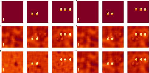
When generating noise, we consider three settings: low, medium, and high signal-to-noise ratio (SNR). First, the noise components are generated from Gaussian random fields using neuRosim and a first-order autoregressive process. At the first time point, we use a 33 × 33 Gaussian random field. The standard deviation is set to 1, and the full-width at half maximum of the Gaussian kernel (FWHM), which controls spatial correlation, is set to 6. At times $T=2,3,\dots ,50$, the noise components are generated recursively by multiplying the T – 1 component by 0.47, and adding an independent Gaussian random field with FWHM = 6. Second, to achieve the desired SNR ratio, we adjust the variance ${\sigma }^2$ of the Gaussian random noise N as follows. Let ${\lambda }_1,{\lambda }_2,\dots ,{\lambda }_Q$ be the nonzero eigenvalues of the covariance matrix of $\mathbf{\text{SM}}$. Then we define $\text{SNR}={\sum }_{i=1}^Q{\lambda }_i/T{\sigma }^2$, and consider $\text{SNR}=0.4$ (low SNR), $\text{SNR}=1.5$ (medium SNR), and $\text{SNR}=3$ (high SNR). To evaluate the performance of each method, we use the scale and permutation invariant root mean squared error (PRMSE) (Risk, Matteson, and Ruppert, 2019).

Since the ICA problem is nonconvex, convergence to a local rather than a global optimum is a well-known issue that can affect estimation accuracy (Risk et al., 2014). We implement both single and 40 random initializations for Sparse ICA, Fast ICA, and Infomax ICA, to examine possible issues with local optima. The results are highly similar in single-subject simulations (See the Web Supplement Section 4.1.1). Moreover, the available implementations of Sparse ICA-EBM and Sparse Fast ICA methods do not allow for multiple random initializations, and modifying these procedures accordingly is not straightforward as they lack an explicit objective function. For fair cross-comparison, we only consider a single initialization for all ICA methods in single-subject simulations.

3.1.2 Results

Figure 1 shows the true source signal matrix S and estimates $\widehat{\mathbf{S}}$ from one replication in the low SNR regime. Sparse ICA recovers the true components (Panel B), while component 2 and component 3 in Infomax ICA (Panel C), Fast ICA-tanh (Panel D), SICA-EBM (Panel E), and Sparse Fast ICA (Panel F) are contaminated by the other components. The remaining inactive pixels for all components using all ICA methods except Sparse ICA are nonzero with contamination from the Gaussian random field noise. We highlight that our Sparse ICA with BIC-selected ν not only selects the true active pixels in estimated ICs but also achieves exact zeros in inactive pixels. Our Sparse ICA achieves high detection performance at the BIC-selected ν, which is measured by Matthew’s correlation coefficient and F1 score (See Web Supplement Section 4.1.2). These measurements for the other methods are all 0 because they do not select for sparsity.

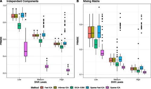
Our Sparse ICA method outperforms the other methods across all SNR settings in both the source signal and mixing matrices estimations (Figure 2(A) and (B), respectively). According to Figure 2(A), the estimation of source signal matrices using all five ICA methods becomes more accurate as the SNR level increases. At each SNR level, Fast ICA and Infomax ICA behave similarly, while SICA-EBM shows a slight improvement Sparse Fast ICA exhibits similar behavior under the low SNR level but becomes unstable in medium and high SNR settings. Sparse Fast ICA involves multiple tuning parameters and stop criteria options. There is no clear way to optimize these arguments, and thus we used the value from the authors’ original paper. Our Sparse ICA demonstrates the largest improvements at the low SNR setting. These substantial improvements imply that when the underlying true source signals are sparse, imposing sparsity constraints leads to better decomposition of source signals. Moreover, accurate estimates of time courses in the mixing matrix will benefit downstream analyses such as brain functional connectivity analysis.

Fig. 2 The PRMSE of estimated source signal matrices ($\widehat{\mathbf{S}}$) and mixing matrices ($\widehat{\mathbf{M}}$). Results represent 100 replications with a single initiation for each SNR level. A: PRMSE of estimated $\widehat{\mathbf{S}}$. B: PRMSE of estimated $\widehat{\mathbf{M}}$.

Table 1 shows the computation time of all five ICA algorithms. Note Sparse ICA is implemented in Rcpp, Fast ICA is implemented in R package fastICA with method=“C”, Infomax ICA is a pure R implementation, while SICA-EBM and Sparse Fast ICA are implemented in MATLAB using their authors’ codes. Sparse ICA is faster than Infomax ICA but is slower than Fast ICA. Sparse Fast ICA is comparable and even faster than Fast ICA, which is probably due to the fact that it’s implemented in MATLAB. However, SICA-EBM is considerably slower than other methods even though it is implemented in MATLAB.

Table 1 Average computation times in seconds over 100 replications for Sparse ICA and other methods.

	Sparse ICA ($\mathsf{\text{Rcpp}}$)	Fast ICA ($\mathsf{\text{Rcpp}}$)	Infomax ICA ($\mathsf{R}$)	SICA-EBM ($\mathsf{\text{MATLAB}}$)	Sparse fast ICA ($\mathsf{\text{MATLAB}}$)
Low SNR	0.0080	0.0022	0.0141	16.0053	0.0055
Medium SNR	0.0079	0.0023	0.0186	22.9243	0.0024
High SNR	0.0081	0.0023	0.0177	19.9347	0.0019
High-dimensional	1.9147	0.4323	2.3359	2233.4951	0.0253

NOTE: SICA-EBM and Sparse fast ICA are implemented in $\mathsf{\text{MATLAB}}$, other ICA methods are in $\mathsf{R}$ and $\mathsf{\text{Rcpp}}$.

In the Web Supplement Section 4.1.3, we examine the setting where the true source signals are non-sparse. Our estimates of source signals using Sparse ICA are less accurate than Fast ICA and Infomax ICA, though more accurate than SICA-EBM and comparable to Sparse Fast ICA (Web Supplement Figure 3(A)). Estimation of the mixing matrix is more robust, as the accuracy of Sparse ICA is similar to Fast ICA and Infomax ICA, and even outperforms Fast ICA in the low SNR setting, while outperforming SICA-EBA and Sparse Fast ICA (Web Supplement Figure 3(B)).

Fig. 3 The true and estimated IC-2 (Default Mode Network A) from a single repetition. A: The true IC-2. B: Sparse ICA. C: Infomax ICA. D: Fast ICA. D: SICA-EBM. F: Sparse Fast ICA.

3.1.3 High-Dimensional Simulation Design

We simulate high-dimensional data that mimics the real fMRI data. We specify three independent components selected from 30 sparse group components in a preliminary analysis of group Sparse ICA on the school-age ABIDE cortical surface fMRI data used in Section 4 with ν = 1. The values of active vertices vary from –1.74 to 5.59, while the values of inactive vertices are set to exact zeros. These three components were used to back-construct the ICA time series of a randomly chosen subject (sub-29286) in the ABIDE data, which were then used as the true time courses. The noise components are generated from the standard normal distribution and then spatially smoothed using the ciftiTools package (Pham, Muschelli, and Mejia, 2022). We simulate 120 time points with SNR = 0.4. The correlations between the true and estimated source signals or rows of the mixing matrices are calculated for each IC as a measure of estimation accuracy.

We implement both single and 40 random initializations for Sparse ICA, Fast ICA, and Infomax ICA. The results are highly similar in single-subject simulations (See the Web Supplement Section 4.2.2). Moreover, due to the difficulties of implementing Sparse ICA-EBM and Sparse Fast ICA methods using multiple random initializations, we only consider the single random initialization versions of all five ICA methods for fair cross-comparison.

3.1.4 Results

Figure 3 shows the second true independent component (IC-2), which is part of the default mode network (DMN) estimated from ABIDE data, as well as corresponding estimates using five ICA methods. Other components are depicted in the Web Supplement Section 4.2.1. Similar to other simulations, all other ICA methods capture the true source signals with noise components in the background, and have similar performance. In contrast, the proposed Sparse ICA is superior by estimating zeros at most of the locations that are truly zero, thus, boosting the accuracy and interpretability of both estimated independent components and the mixing matrix. The median Matthew’s correlation at the selected ν is 0.730, and the median F1 score is 0.983 (Web Supplement Table 1). Additionally, most true nonzeros are nonzero in the Sparse ICA estimates, although a few areas with true nonzeros that are close to zero are shrunk to zero in our Sparse ICA (examples are in the frontal lobe).

As shown in Table 2, our Sparse ICA method outperforms other ICA algorithms in recovering the source signals across all independent components in high-dimensional simulations. The behaviors of Fast ICA, Infomax ICA, and Sparse Fast ICA are similar, while Sparse ICA achieves improved estimation for both source signals and mixing matrices. SICA-EBM also shows slight improvements for IC 2 and 3 relative to Fast ICA and Infomax ICA. As shown in the last row in Table 1, our Sparse ICA method takes about 2 seconds to recover ICs, which is faster than Infomax ICA and SICA-EBM but slower than Fast ICA and Sparse Fast ICA.

Table 2 Mean (standard deviation) of the correlations between the true and estimated source signals and mixing matrices based on different ICA methods with 100 simulation runs in the high-dimensional setting.

Correlations	Sparse ICA	Fast ICA	Infomax ICA	SICA-EBM	Sparse Fast ICA
IC1—Source	0.975(0.002)	0.927(0.003)	0.929(0.003)	0.903(0.108)	0.921(0.036)
IC2—Source	0.969(0.002)	0.917(0.003)	0.918(0.003)	0.944(0.002)	0.917(0.003)
IC3—Source	0.983(0.002)	0.920(0.003)	0.921(0.003)	0.949(0.002)	0.913(0.037)
IC1—Mixing	0.997(0.000)	0.995(0.001)	0.994(0.001)	0.996(0.001)	0.989(0.049)
IC2—Mixing	0.996(0.001)	0.993(0.001)	0.992(0.001)	0.994(0.002)	0.993(0.001)
IC3—Mixing	0.997(0.000)	0.995(0.001)	0.994(0.001)	0.883(0.257)	0.986(0.054)

Bold values indicate the method that has the highest correlation with the truth.

In the Web Supplement Section 4.2.3, we examine the non-sparse case by setting the true components to be the non-sparse Fast ICA solution on ABIDE data. Unsurprisingly, Sparse ICA does worse than other methods on the source signals when the truth is non-sparse. However, on mixing matrices, Sparse ICA is highly accurate and performs similarly to Fast ICA and Infomax ICA.

3.2 Group Level Simulations

3.2.1 Simulation Design

We use 20 subjects, and simulate 3 group components, 22 individual components, and 25 Gaussian noise components for each subject. Web Supplement Section 5.2 contains example components. The group components have active pixels in the shape of “1”, “2 2” and “3 3 3” with values varying from 0.5 to 1. The inactive pixels are exact zeros. Individual components were simulated from Gamma random fields with shape parameter 0.02 and rate parameter ${10}^{-4}$. The noise components were simulated from standard Gaussian random fields. All the random fields were generated using the R package neuRosim (Welvaert et al., 2011). While we do not enforce the orthogonality of components, the model assumptions are approximately met since the active areas of group components are disjoint and the individual components are independent. The time courses with 50 time units in the mixing matrices were simulated using AR(1) processes with $\varphi =0.47$. Thus, subjects in the group have different randomly generated individual components and corresponding time series.

To control the strength levels of signals and noises, we controlled the proportion of variance from the group components, individual components, and the Gaussian noise components. In this group-level simulation, we focused on the signal-to-noise ratio (SNR) between group components and noise components. The definition of SNR is described in Section 3.1. We defined three SNR settings, low SNR (proportion of variance in group, individual, and noise components = 35%, 15%, 50%), medium SNR (variance proportion = 40%, 20%, 40%), and high SNR (variance proportion = 50%, 20%, 30%). We use PRMSE, which is also defined in Section 3.1, to evaluate the performance of each group method. Since each subject has its own estimated mixing matrix, we use the average PRMSE of mixing matrices in the group as the measurement of mixing matrix estimation.

Subject-level PCA in which the number of PCs selected to retain at least 80% of the total variance was conducted for each subject, and the subject PCs were then concatenated together for input to Sparse ICA. The group Fast ICA and group Infomax ICA were implemented based on the same procedure to ensure fair comparisons. After extracting group components, the corresponding subject-specific time courses were back-constructed. We then calculated the PRMSE between estimated group components and true group components, and the group average PRMSE between estimated subject-specific mixing matrices and true mixing matrices.

Unlike the single-subject simulations, we found that employing multiple random initializations improved accuracy. Since the available implementations of SICA-EBM and Sparse Fast ICA do not allow for multiple random initializations, we did not estimate group ICs for SICA-EBM or Sparse Fast ICA. Sparse ICA, Fast ICA, and Infomax ICA were repeated under 50 replications for each SNR setting with 40 random initializations.

We also record computation times for all group ICA methods. Since there is not a multiple initialization option in the R package fastICA, we wrote a for-loop in R to select the estimate with the highest objective function value. In contrast, the implementation of our Sparse ICA method implements a for-loop in Rcpp, and is thus much faster than Fast ICA with the for-loop in $\mathsf{R}$. For a fair comparison, we report the computation time of ICA methods with a single initialization.

3.2.2 Results

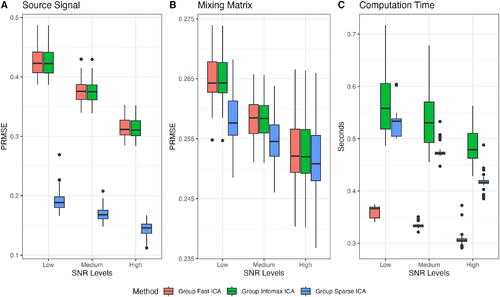
The accuracy of the estimated components in group Fast ICA and group Infomax ICA is similar, while our group Sparse ICA demonstrates substantial improvements across all SNR settings (Panel A in Figure 4). As for the estimation of the mixing matrix in Panel B, our group Sparse ICA shows improvements over group Fast ICA and group Infomax ICA in the low and medium SNR settings, while the mixing matrix accuracy is similar in the high SNR setting. In Panel C, our group Sparse ICA is computationally faster and more stable than group Infomax ICA, but is slower than group Fast ICA.

Fig. 4 The PRMSE of estimated group components (${\widehat{\mathbf{S}}}_g$) and mixing matrices (${\widehat{\mathbf{M}}}_i,i=1,2,\dots ,20$). Results represent 50 replications with 40 random initializations for each SNR level. A: PRMSE between estimated ${\widehat{\mathbf{S}}}_g$ and true S_g. B: Average PRMSE between estimated subject ${\widehat{\mathbf{M}}}_i$ and true ${\mathbf{M}}_i,i=1,2,\dots ,20$. C: The computation time of a single initialization in seconds.

4 Application to Cortical Surface fMRI Data

4.1 Data and Methods

We processed resting-state fMRI data from school-age children selected from the Autism Brain Imaging Data Exchange (ABIDE) using a cortical surface fMRI pipeline. We used both the ABIDE-I (Di Martino, Al, and Milham, 2013) and ABIDE-II datasets (Di Martino et al., 2017), and selected 396 children (103 females) aged 8–13 (mean = 10.4, sd = 1.4) from two sites: the Kennedy Krieger Institute (KKI) and NYU Langone Medical Center (NYU). The sample included 252 typically developing (TD) (78 females) and 144 ASD children (25 females). Details on the preprocessing are in Web Supplement Section 7.1. Nineteen participants were excluded due to poor T1 images or cortical registration failure. We then adopted a motion quality control criterion based on Power et al. (2014) in which participants were excluded if they had less than 5 min of data with framewise displacement less than 0.2 mm. Consequently, 65 participants were marked as having excessive motion. In total, 84 participants were removed in the quality control procedure.

We applied group Sparse ICA using Web Supplement Algorithm 1 to our pre-processed cortical surface fMRI data that passed manual inspection and motion quality control criteria (n = 312). In ICA, it is typical to normalize the time course for each voxel to have zero mean and unit variance (normalize each row) before centering and scaling each image (normalize each column). We use an iterative approach with five iterations to achieve standardization across both rows and columns (Risk and Gaynanova, 2021). The subject-level dimension reduction step was performed by PCA with 85 principle components retained for each participant (Nebel et al., 2022), see Web Supplement Section 7.3. Thirty group components as in (Lombardo et al., 2019; Nebel et al., 2022) were extracted in the final Sparse ICA step with the tuning parameter ν = 2 selected by our proposed BIC-like criterion (Web Supplement Figure 18). We found that results were sensitive to initialization (see Web Supplement Section 7.4). We ran the algorithms for two independent runs with 40 random initializations each. The argmax from these two runs were equivalent, indicating a sufficient number of restarts. Since the sign of the components is not identifiable, we choose the sign to result in positive skewness (Eloyan and Ghosh, 2013). We also examined the sensitivity to the specified number of components and found that Sparse ICA estimates on ABIDE data are similar across a range of specifications, in agreement with what we also observed in simulations (Web Supplement Section 6.2).

We used the subject-specific time courses to construct the subject-specific Pearson correlation matrices. We Fisher z-transformed the correlation matrices and extracted the lower triangle resulting in 435 edges. We applied ComBat for site harmonization (Yu et al., 2018) in which “site” was a factor with three levels (NYU, KKI-8 channel, KKI-32 channel) with the following covariates: diagnosis, mean framewise displacement, full-scale intelligence quotient, autism diagnostic observation schedule (a measure of autism severity), stimulant medication status, non-stimulant medication status, proportion of framewise displacement greater than 0.2 mm, proportion of root mean square displacement greater than 0.25 mm, handedness (right or left handed), age at scan, and sex. We included all variables used in downstream analyses in the ComBat step in order to avoid over-correction of site effects.

Although the exclusion of participants with excessive motion can improve the quality of resting-state fMRI data, it may alter the distribution of clinically relevant covariates. We follow Nebel et al. (2022) to account for possible demographic confounders and selection biases due to motion exclusion criteria. Details are in Web Supplement Section 7.9 and summarized here. We use the augmented inverse probability of inclusion weighted estimator (AIPWE) (Robins, Rotnitzky, and Zhao, 1994) to estimate the debiased group difference in functional connectivity between ASD and TD children. The propensity model and the outcome model were fitted using the super learner algorithm (Van der Laan, Polley, and Hubbard, 2007). The learners for the propensity model included multivariate adaptive regressions splines, lasso, generalized additive models, generalized linear models, random forests, step-wise regression, xgboost, and mean. In the outcome model, we added ridge regression and support vector machines. The same set of predictors was used in both the propensity and outcome models, including sex, age at scan, FIQ, handedness, diagnosis, stimulant medication status, non-stimulant medication status, and ADOS. p-values were corrected for multiple comparisons using the false discovery rate.

4.2 Results

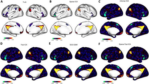
The functional connectivity between IC-18 and IC-20 and the functional connectivity between IC-5 and IC-13 were significantly lower in ASD than TD at FDR = 0.05 (adjusted p-value = 0.011). We depict these components in the top two rows of Figure 5 as estimated using Sparse ICA (A and B) and the corresponding matched components from Fast ICA (C and D), with Infomax components in the Web Supplement Section 7.8. The z-scores for all AIPWE-adjusted group differences are depicted in the Web Supplement Section 7.9. Sparse ICA identifies activated vertices as nonzero values with inactive vertices being exact zeros. Interestingly, all of the nonzero values are positive. In contrast, the matched components from Fast ICA are dense with both positive and negative values. The Sparse ICA components represent vertices that co-activate, whereas the Fast ICA components include dense locations with opposing directions of “activation.”

Fig. 5 ICs selected for significant edge differences between ASD and TD. Columns A and B: Sparse ICA. Column A row 1 (IC-18): posterior cingulate and precuneus areas of the default mode network. Column A row 2 (IC-20): medial prefrontal regions of the default mode. Column A row 3: subject-specific correlations between IC time courses with the AIPWE-adjusted estimate of the means (red square, FDR-adjusted p = 0.011). Column B row 1 (IC-13): temporal parietal junction. Column B row 2 (IC-5): frontal areas of executive function. Column B row 3: subject-specific correlations (FDR-adjusted p = 0.011). Columns C and D: matched components from Fast ICA.

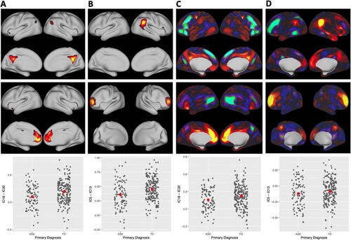
By examining the overlap between the nonzero ICs and the resting-state networks from Yeo et al. (2011), IC-18 corresponds to the medial posterior default mode network, highlighting regions in the posterior cingulate cortex and precuneus, and IC-20 corresponds to the medial prefrontal cortex region of the default mode network. Alterations in the default mode network were also found in an analysis of all ages in the ABIDE-I dataset using a seed-based correlation analysis (Di Martino, Al, and Milham, 2013). Our sparse components depicted in A and B are more easily related to the seed-based correlation analyses in Di Martino, Al, and Milham (2013), since a positive correlation between IC-18 and IC-20 is interpreted as increased brain connectivity in the same way as a positive correlation in a seed-based analysis is interpreted as increased brain connectivity. In contrast, the matched components in Fast ICA in Panel C contain negative values in the components as well, such that an increased correlation between time courses means opposite things for the locations with positive versus negative values, which is scientifically harder to understand. IC-13 (top row, column B) corresponds to portions of the temporal parietal junction, which is associated with salience, control, auditory, and default mode networks, and IC-5 corresponds to the frontoparietal network (middle row, column B), which is associated with executive function.

5 Discussion

In this work, we propose a new ICA method that estimates sparse independent components leveraging a relax-and-split algorithm. Our method is very fast and can be easily applied to big data. In contrast to the common practice of post-hoc thresholding the components, our method estimates sparse components and corresponding time courses directly via the Laplace density. Through simulation studies, we show that the proposed method can accurately select nonzero spatial locations and improve accuracy. In addition, our analysis of the resting state fMRI data from the school-age children demonstrates the ability of our Sparse ICA method to handle high-dimensional fMRI data and produce sparse spatial maps that are easy to interpret.

Some studies suggest that ASD is characterized by overall hypoconnectivity alongside specific local hyperconnectivity (Di Martino, Al, and Milham, 2013; Lord et al., 2018). Other authors emphasize that no clear picture has emerged from neuroimaging (Müller and Fishman, 2018). Using Sparse ICA, we find that anterior-to-posterior functional connectivity in the default mode network is lower in autistic children. This altered connectivity may relate to atypical integration of information pertaining to self-referential thought (Padmanabhan et al., 2017). In an analysis of the first ABIDE data release including adults and children (ages 7–64), Di Martino, Al, and Milham (2013) also found posterior to anterior hypoconnectivity in the default mode network. Second, we found reduced functional connectivity between the temporal parietal junction and frontal areas of executive function, which may also be related to impairment in information integration (Lord et al., 2020). One strength of our analysis is that we focus on school-age children, which is an important age for behavioral interventions. Another strength is that we excluded high motion participants and used the debiased group difference to account for possible selection bias (Nebel et al., 2022). It is scientifically important to note that the results are highly variable. ASD is a very heterogeneous disorder. As of 2013, ASD is a single spectrum that includes Asperger’s syndrome and pervasive developmental disorder not otherwise specified (Lord et al., 2018). Our findings represent general patterns in autism rather than biomarkers. Studies examining autism subtypes hold promise for translational findings (Müller and Fishman, 2018). Lombardo et al. (2019) found large effect sizes between the default mode and attention networks in a subtype with social-visual engagement difficulties. We hope future studies will combine Sparse ICA with subtype analysis to improve our understanding of brain connectivity in autism.

There is disagreement about whether ICA algorithms applied to fMRI data are targeting independence or in fact indirectly approximating sparse latent factors. Daubechies et al. (2009) argued that the most used ICA algorithms, including Infomax ICA and Fast ICA, handle the sparsity rather than the independence in brain fMRI studies. However, Calhoun et al. (2013) argued that ICA algorithms do indeed estimate maximally independent components. Our Sparse ICA method contributes to this topic by formally establishing a mathematical framework that directly introduces sparsity to the independent components, and finds the balance between the independence and sparsity of the source signals.

Compared to existing work, the use of the relax-and-split algorithm in our Sparse ICA method overcomes challenges of the non-smooth objective function and orthogonal constraints. Our approach achieves exact zeros, which contrasts with SICA-EBM and Sparse Fast ICA. Moreover, there is only one tuning parameter controlling the level of independence and sparsity in our method. In the existing sparse methods in ICA, there are multiple tuning parameters whose selection procedures are ambiguous, and the resulting components do not contain exact zeros. Furthermore, we show that the computation time of our Sparse ICA method is much shorter than Infomax ICA and SICA-EBM, and easily applied to high dimensions, where components are estimated in seconds.

There are a number of limitations of our approach and directions for future research. We follow the group ICA framework popularized in GIFT (Rachakonda et al., 2007) by assuming the subjects in the group analysis share the same group independent components with different corresponding time courses, which has been previously applied in functional connectivity studies of autistic children (Lombardo et al., 2019; Lidstone et al., 2021; Nebel et al., 2022). A limitation of our approach is that there is no variation in components across subjects. Additionally, we use regression to estimate subject time courses. It would be preferable to formulate a unified statistical model with population and subject-level effects. Future work can investigate the incorporation of random effects as in Guo and Tang (2013). However, these methods tend to be computationally costly as their complexity grows exponentially with the number of components. Ultimately, widespread adoption of ICA methods depends on scientists’ assessments of possible, but unknown, benefits of statistical improvements with the computational costs, which are known.

Another limitation is that we selected the number of components in our data analysis based on the results from previous studies with similar data (Lombardo et al., 2019; Nebel et al., 2022), rather than a data-driven approach. We have found that data-driven selection of the number of components using information criteria as in GIFT or Melodic can produce variable estimates. In fact, it is common for the authors of the software packages that provide automated dimension estimation to specify the number of group components (Smith et al., 2015; Du et al., 2020). Recent statistical papers on ICA also specify the number of group components (Guo and Tang, 2013; Mejia et al., 2020). In general, automated methods do not work well when there is a small gap between the eigenvalues in the principal subspace and the noise variance, which is common in fMRI. We made progress on this issue in the related class of models in LNGCA using a parametric bootstrap accounting for spatially correlated noise components (Zhao et al., 2022). A similar procedure could be pursued here by using a parametric bootstrap to estimate the null distribution of eigenvalues of spatially correlated noise components, but again the widespread implementation may be limited by computational costs.

Supplementary Materials

The Web Supplement contains detailed derivations of alternating updates, the proof of algorithmic convergence, additional simulation results and the real data analysis. $\mathsf{R}$-package SparseICA can be obtained from https://github.com/thebrisklab/SparseICA.

Acknowledgments

The authors are thankful to Dr. Peng Zheng for his help in the development and implementation of the relax-and-split ICA algorithm. We are also thankful to Sijian Fan for his help on $\mathsf{R}$ implementations of the relax-and-split algorithm and to Jialu Ran and Liangkang Wang for help with the data processing. We also thank Dr. Lei Zhou for computing support.

Disclosure Statement

The authors report there are no competing interests to declare.

Additional information

Funding

This work was supported by the National Institute of Mental Health of the National Institutes of Health under award number R01 MH129855 (BR), NSF DMS 2044823 (IG), and the Washington Research Foundation Data Science Professorship (AA).

References

- Allen, G. I., and Maletić-Savatić, M. (2011), “Sparse Non-negative Generalized PCA with Applications to Metabolomics,” Bioinformatics, 27, 3029–3035. DOI: 10.1093/bioinformatics/btr522.
- Babaie-Zadeh, M., Jutten, C., and Mansour, A. (2006), “Sparse ICA via Cluster-Wise PCA,” Neurocomputing, 69, 1458–1466. DOI: 10.1016/j.neucom.2005.12.022.
- Beckmann, C. F., and Smith, S. M. (2004), “Probabilistic Independent Component Analysis for Functional Magnetic Resonance Imaging,” IEEE Transactions on Medical Imaging, 23, 137–152. DOI: 10.1109/TMI.2003.822821.
- Bell, A. J., and Sejnowski, T. J. (1995), “An Information-Maximization Approach to Blind Separation and Blind Deconvolution,” Neural Computation, 7, 1129–1159. DOI: 10.1162/neco.1995.7.6.1129.
- Boukouvalas, Z., Levin-Schwartz, Y., Calhoun, V. D., and Adal i, T. (2018), “Sparsity and Independence: Balancing Two Objectives in Optimization for Source Separation with Application to fMRI Analysis,” Journal of the Franklin Institute, 355, 1873–1887. DOI: 10.1016/j.jfranklin.2017.07.003.
- Calhoun, V. D., Adali, T., Pearlson, G. D., and Pekar, J. J. (2001), “A Method for Making Group Inferences from Functional MRI Data Using Independent Component Analysis,” Human Brain Mapping, 14, 140–151. DOI: 10.1002/hbm.1048.
- Calhoun, V. D., Potluru, V. K., Phlypo, R., Silva, R. F., Pearlmutter, B. A., Caprihan, A., et al. (2013), “Independent Component Analysis for Brain fMRI Does Indeed Select for Maximal Independence,” PloS One, 8, e73309. DOI: 10.1371/journal.pone.0073309.
- Damoiseaux, J. S., Rombouts, S., Barkhof, F., Scheltens, P., Stam, C. J., Smith, S. M., et al. (2006), “Consistent Resting-State Networks Across Healthy Subjects,” Proceedings of the National Academy of Sciences, 103, 13848–13853. DOI: 10.1073/pnas.0601417103.
- Daubechies, I., Roussos, E., Takerkart, S., Benharrosh, M., Golden, C., D’ardenne, K., et al. (2009), “Independent Component Analysis for Brain fMRI Does Not Select for Independence,” Proceedings of the National Academy of Sciences, 106, 10415–10422. DOI: 10.1073/pnas.0903525106.
- Di Martino, A., Al, E., and Milham, M. P. (2013), “The Autism Brain Imaging Data Exchange: Towards a Large-Scale Evaluation of the Intrinsic Brain Architecture in Autism,” Molecular Psychiatry, 19, 659–667. DOI: 10.1038/mp.2013.78.
- Di Martino, A., O’connor, D., Chen, B., Alaerts, K., Anderson, J. S., Assaf, M., et al. (2017), “Enhancing Studies of the Connectome in Autism Using the Autism Brain Imaging Data Exchange II,” Scientific Data, 4, 1–15. DOI: 10.1038/sdata.2017.10.
- Du, Y., Fu, Z., Sui, J., Gao, S., Xing, Y., Lin, D., et al. (2020), “Neuromark: An Automated and Adaptive ICA based Pipeline to Identify Reproducible fMRI Markers of Brain Disorders,” NeuroImage: Clinical, 28, 102375. DOI: 10.1016/j.nicl.2020.102375.
- Eloyan, A., and Ghosh, S. K. (2013), “A Semiparametric Approach to Source Separation Using Independent Component Analysis,” Computational Statistics & Data Analysis, 58, 383–396. DOI: 10.1016/j.csda.2012.09.012.
- Erhardt, E. B., Rachakonda, S., Bedrick, E. J., Allen, E. A., Adali, T., and Calhoun, V. D. (2011), “Comparison of Multi-Subject ICA Methods for Analysis of fMRI Data,” Human Brain Mapping, 32, 2075–2095. DOI: 10.1002/hbm.21170.
- Erichson, N. B., Zheng, P., Manohar, K., Brunton, S. L., Kutz, J. N., and Aravkin, A. Y. (2020), ‘Sparse Principal Component Analysis via Variable Projection,” SIAM Journal on Applied Mathematics, 80, 977–1002. DOI: 10.1137/18M1211350.
- Fan, S. (2020), “Improved Algorithm for Independent Component Analysis (ICA) with the Relax and Split Approximation,” Emory Theses and Dissertations.
- Ge, R., Wang, Y., Zhang, J., Yao, L., Zhang, H., and Long, Z. (2016), “Improved Fastica Algorithm in fMRI Data Analysis Using the Sparsity Property of the Sources,” Journal of Neuroscience Methods, 263, 103–114. DOI: 10.1016/j.jneumeth.2016.02.010.
- Guo, Y., and Tang, L. (2013), “A Hierarchical Model for Probabilistic Independent Component Analysis of Multi-Subject fMRI Studies,” Biometrics, 69, 970–981. DOI: 10.1111/biom.12068.
- Hyvarinen, A. (1999), “Fast and Robust Fixed-Point Algorithms for Independent Component Analysis,” IEEE Transactions on Neural Networks, 10, 626–634. DOI: 10.1109/72.761722.
- Lee, H., Battle, A., Raina, R., and Ng, A. (2006), “Efficient Sparse Coding Algorithms,” in Advances in Neural Information Processing Systems (Vol. 19).
- Li, Y.-O., Adal i, T., and Calhoun, V. D. (2007), “Estimating the Number of Independent Components for Functional Magnetic Resonance Imaging Data,” Human Brain Mapping, 28, 1251–1266. DOI: 10.1002/hbm.20359.
- Lidstone, D. E., Rochowiak, R., Mostofsky, S. H., and Nebel, M. B. (2021), “A Data Driven Approach Reveals that Anomalous Motor System Connectivity is Associated with the Severity of Core Autism Symptoms,” Autism Research, 1–18. DOI: 10.1002/aur.2476.
- Lombardo, M. V., Eyler, L., Moore, A., Datko, M., Carter Barnes, C., Cha, D., et al. (2019), “Default Mode-Visual Network Hypoconnectivity in An Autism Subtype with Pronounced Social Visual Engagement Difficulties,” elife, 8, e47427. DOI: 10.7554/eLife.47427.
- Long, Q., Bhinge, S., Levin-Schwartz, Y., Boukouvalas, Z., Calhoun, V. D., and Adal i, T. (2019), “The Role of Diversity in Data-Driven Analysis of Multi-Subject fMRI Data: Comparison of Approaches based on Independence and Sparsity Using Global Performance Metrics,” Human Brain Mapping, 40, 489–504. DOI: 10.1002/hbm.24389.
- Lord, C., Brugha, T. S., Charman, T., Cusack, J., Dumas, G., Frazier, T., Jones, E. J., Jones, R. M., Pickles, A., State, M. W., et al. (2020), “Autism Spectrum Disorder,” Nature Reviews Disease Primers, 6, 1–23. DOI: 10.1038/s41572-019-0138-4.
- Lord, C., Elsabbagh, M., Baird, G., and Veenstra-Vanderweele, J. (2018), “Autism Spectrum Disorder,” The Lancet, 392, 508–520. DOI: 10.1016/S0140-6736(18)31129-2.
- Lukemire, J., Pagnoni, G., and Guo, Y. (2023), “Sparse Bayesian Modeling of Hierarchical Independent Component Analysis: Reliable Estimation of Individual Differences in Brain Networks,” Biometrics, 79, 3599–3611. DOI: 10.1111/biom.13867.
- Mejia, A. F., Nebel, M. B., Wang, Y., Caffo, B. S., and Guo, Y. (2020), “Template Independent Component analysis: Targeted and Reliable Estimation of Subject-Level Brain Networks Using Big Data Population Priors,” Journal of the American Statistical Association, 115, 1151–1177. DOI: 10.1080/01621459.2019.1679638.
- Minka, T. (2000), “Automatic Choice of Dimensionality for PCA,” in Advances in Neural Information Processing Systems (Vol. 13).
- Müller, R.-A., and Fishman, I. (2018), “Brain Connectivity and Neuroimaging of Social Networks in Autism,” Trends in Cognitive Sciences, 22, 1103–1116. DOI: 10.1016/j.tics.2018.09.008.
- Nebel, M. B., Lidstone, D. E., Wang, L., Benkeser, D., Mostofsky, S. H., and Risk, B. B. (2022), “Accounting for Motion in Resting-State fMRI: What Part of the Spectrum are We Characterizing in Autism Spectrum Disorder?” NeuroImage, 257, 119296. DOI: 10.1016/j.neuroimage.2022.119296.
- Padmanabhan, A., Lynch, C. J., Schaer, M., and Menon, V. (2017), “The Default Mode Network in Autism,” Biological Psychiatry: Cognitive Neuroscience and Neuroimaging, 2, 476–486. DOI: 10.1016/j.bpsc.2017.04.004.
- Pham, D. D., Muschelli, J., and Mejia, A. F. (2022), “ciftitools: A Package for Reading, Writing, Visualizing, and Manipulating Cifti Files in r,” NeuroImage, 250, 118877. DOI: 10.1016/j.neuroimage.2022.118877.
- Power, J. D., Mitra, A., Laumann, T. O., Snyder, A. Z., Schlaggar, B. L., and Petersen, S. E. (2014), “Methods to Detect, Characterize, and Remove Motion Artifact in Resting State fMRI,” NeuroImage, 84, 320–341. DOI: 10.1016/j.neuroimage.2013.08.048.
- Rachakonda, S., Egolf, E., Correa, N., and Calhoun, V. (2007), “Group ICA of fMRI Toolbox (gift) Manual,” Dostupnez [cit 2011-11-5].
- Risk, B. B., and Gaynanova, I. (2021), “Simultaneous Non-Gaussian Component Analysis (sing) for Data Integration in Neuroimaging,” The Annals of Applied Statistics, 15, 1431–1454. DOI: 10.1214/21-AOAS1466.
- Risk, B. B., Matteson, D. S., and Ruppert, D. (2019), “Linear Non-Gaussian Component Analysis via Maximum Likelihood,” Journal of the American Statistical Association, 114, 332–343. DOI: 10.1080/01621459.2017.1407772.
- Risk, B. B., Matteson, D. S., Ruppert, D., Eloyan, A., and Caffo, B. S. (2014), “An Evaluation of Independent Component Analyses with an Application to Resting-State fMRI,” Biometrics, 70, 224–236. DOI: 10.1111/biom.12111.
- Robins, J. M., Rotnitzky, A., and Zhao, L. P. (1994), “Estimation of Regression Coefficients When Some Regressors are not always Observed,” Journal of the American statistical Association, 89, 846–866. DOI: 10.1080/01621459.1994.10476818.
- Sadaghiani, S., Hesselmann, G., Friston, K. J., and Kleinschmidt, A. (2010), “The Relation of Ongoing Brain Activity, Evoked Neural Responses, and Cognition,” Frontiers in Systems Neuroscience, 4, 1424. DOI: 10.3389/fnsys.2010.00020.
- Shen, H., and Huang, J. Z. (2008), ‘Sparse Principal Component Analysis via Regularized Low Rank Matrix Approximation,” Journal of Multivariate Analysis, 99, 1015–1034. DOI: 10.1016/j.jmva.2007.06.007.
- Smith, S. M., Jenkinson, M., Woolrich, M. W., Beckmann, C. F., Behrens, T. E., Johansen-Berg, H., et al. (2004), “Advances in Functional and Structural MR Image Analysis and Implementation as fsl,” Neuroimage, 23, S208–S219. DOI: 10.1016/j.neuroimage.2004.07.051.
- Smith, S. M., Nichols, T. E., Vidaurre, D., Winkler, A. M., Behrens, T. E., et al. (2015), “A Positive-Negative Mode of Population Covariation Links Brain Connectivity, Demographics and Behavior,” Nature Neuroscience, 18, 1565–1567. DOI: 10.1038/nn.4125.
- Smith, S. M., Vidaurre, D., Beckmann, C. F., Glasser, M. F., et al. (2013), “Functional Connectomics from Resting-State fMRI,” Trends in Cognitive Sciences, 17, 666–682. DOI: 10.1016/j.tics.2013.09.016.
- Sobczyk, P., Bogdan, M., and Josse, J. (2017), “Bayesian Dimensionality Reduction with PCA Using Penalized Semi-integrated Likelihood,” Journal of Computational and Graphical Statistics, 26, 826–839. DOI: 10.1080/10618600.2017.1340302.
- Van der Laan, M. J., Polley, E. C., and Hubbard, A. E. (2007), “Super Learner,” Statistical Applications in Genetics and Molecular Biology, 6, 1–21. DOI: 10.2202/1544-6115.1309.
- Wei, T. (2015), “A Convergence and Asymptotic Analysis of the Generalized Symmetric {FastICA} Algorithm,” IEEE Transactions on Signal Processing, 63, 6445–6458. DOI: 10.1109/TSP.2015.2468686.
- Welvaert, M., Durnez, J., Moerkerke, B., Verdoolaege, G., and Rosseel, Y. (2011), “neurosim: An r Package for Generating fMRI Data,” Journal of Statistical Software, 44, 1–18. DOI: 10.18637/jss.v044.i10.
- Yeo, B. T., Krienen, F. M., Sepulcre, J., Sabuncu, M. R., Lashkari, D., Hollinshead, M. et al. (2011), “The Organization of the Human Cerebral Cortex Estimated by Intrinsic Functional Connectivity,” Journal of Neurophysiology, 10, 1125–1165. DOI: 10.1152/jn.00338.2011.
- Yu, M., Linn, K. A., Cook, P. A., Phillips, M. L., McInnis, M., Fava, M. et al. (2018), “Statistical Harmonization Corrects Site Effects in Functional Connectivity Measurements from Multi-Site fMRI Data,” Human Brain Mapping, 39, 4213–4227. DOI: 10.1002/hbm.24241.
- Zhao, Y., Matteson, D. S., Mostofsky, S. H., Nebel, M. B., and Risk, B. B. (2022), “Group Linear Non-Gaussian Component Analysis with Applications to Neuroimaging,” Computational Statistics & Data Analysis, 171, 107454. DOI: 10.1016/j.csda.2022.107454.
- Zheng, P., and Aravkin, A. (2020), “Relax-and-Split Method for Nonconvex Inverse Problems,” Inverse Problems, 36, 095013. DOI: 10.1088/1361-6420/aba417.
- Zou, H., Hastie, T., and Tibshirani, R. (2006), “Sparse Principal Component Analysis,” Journal of Computational and Graphical Statistics, 15, 265–286. DOI: 10.1198/106186006X113430.