Synthetic likelihood in misspecified models

Abstract

Bayesian synthetic likelihood is a widely used approach for conducting Bayesian analysis in complex models where evaluation of the likelihood is infeasible but simulation from the assumed model is tractable. We analyze the behaviour of the Bayesian synthetic likelihood posterior when the assumed model differs from the actual data generating process. We demonstrate that the Bayesian synthetic likelihood posterior can display a wide range of non-standard behaviours depending on the level of model misspecification, including multimodality and asymptotic non-Gaussianity. Our results suggest that likelihood tempering, a common approach for robust Bayesian inference, fails for synthetic likelihood whilst recently proposed robust synthetic likelihood approaches can ameliorate this behavior and deliver reliable posterior inference under model misspecification. All results are illustrated using a simple running example.

Keywords:

• Synthetic likelihood
• Approximate Bayesian computation
• Model misspecification
• Likelihood tempering

Disclaimer

As a service to authors and researchers we are providing this version of an accepted manuscript (AM). Copyediting, typesetting, and review of the resulting proofs will be undertaken on this manuscript before final publication of the Version of Record (VoR). During production and pre-press, errors may be discovered which could affect the content, and all legal disclaimers that apply to the journal relate to these versions also.

1 Introduction

Approximate Bayesian methods, sometimes called likelihood-free methods, have become a common approach to conduct Bayesian inference in situations where the likelihood function is intractable. Two of the most prominent statistical methods in this paradigm are approximate Bayesian computation, see Marin et al. (2012) for a review and Sisson et al. (2018) for a handbook treatment, and the method of synthetic likelihood (Wood, 2010). Synthetic likelihood-based inference is often conducted by placing a prior over the unknown model parameters and using Markov chain Monte Carlo methods to sample the resulting posterior. Throughout the remainder we refer to such methods as Bayesian synthetic likelihood, and refer to Price et al. (2018) for an introduction.

The goal of both approximate Bayesian computation (ABC) and Bayesian synthetic likelihood (BSL) is to conduct inference on the unknown model parameters by simulating summary statistics under the assumed model and matching them against observed summaries calculated from the data. The simulated summary statistics are used to construct an estimate of the likelihood, which is then used to conduct posterior inference on the model unknowns. While ABC implicitly constructs a nonparametric estimate of the likelihood for the summaries, synthetic likelihood uses a Gaussian approximation with an estimated mean and variance.

As these methods have grown in prominence, much research has been conducted to understand the benefits and disadvantages of different approximate Bayesian approaches. In terms of statistical regularity, i.e., large sample behavior, the method of approximate Bayesian computation behaves quite regularly in the context of correct model specification (see, e.g., Li and Fearnhead, 2018, and Frazier et al., 2018), with Frazier et al. (2022) demonstrating that BSL displays similar large sample behavior to ABC, while scaling to higher-dimensional summaries more easily than simple implementations of ABC. For a more in-depth comparison of ABC and BSL, we refer to Section 3.1.3 of Martin et al. (2023).

The goal of both methods is to conduct inference in models that are so complicated that the resulting likelihood is intractable. However, models are only ever an approximation of reality and, thus, correct specification is unlikely. Hence, for a diverse collection of summary statistics, it is unlikely that the assumed model can exactly match all the summaries calculated from the observed data; with this problem likely exacerbated in early phases of model exploration, design, and formulation. When the summaries simulated under the assumed model cannot match the observed summaries for any value of the unknown model parameters, we say that the model is misspecified. This notion of misspecification is consistent with previous analyses of misspecification in ABC (see, e.g., Marin et al., 2014, and Frazier et al., 2020).

Several authors have now discussed the impacts of model misspecification in likelihood-based Bayesian inference (see, e.g., Kleijn and van der Vaart, 2012, Miller and Dunson, 2019, Bhattacharya et al., 2019), and it is known that ABC posteriors display non-standard asymptotic behaviors in misspecified models (Frazier et al., 2020). Given the links between ABC and BSL, it is critical for us to understand the behavior of the BSL posterior in misspecified models. However, we are unaware of any research that rigorously characterises the behavior of BSL under model misspecification.

The need to theoretically examine the behavior of the BSL posterior in misspecified models is also motivated by the empirical analysis carried out in Frazier and Drovandi (2021), where the authors present an empirical example showing that the BSL posterior displays non-standard behavior at a small sample size. Critically, Frazier and Drovandi (2021) did not explore whether this behavior abated as the sample size increased, or whether it was an artefact of their Monte Carlo approximation; nor did the authors explore the mechanism causing this non-standard posterior behavior, or present any theoretical results on the behavior of the BSL posterior in misspecified models.

In this manuscript we make four contributions to the literature on approximate Bayesian methods, and BSL methods more particularly. Our first contribution is to formally demonstrate that the BSL posterior is sensitive to model misspecification: depending on the nature of the model misspecification, we prove that the BSL posterior can display non-standard asymptotic concentration or standard (i.e., Gaussian) concentration. These results deviate from those in correctly specified models, where Frazier et al. (2022) demonstrate that the BSL posterior displays standard concentration.¹

Our second contribution is to categorise the wide behaviours that the BSL posterior can present in misspecified models, which we illustrate empirically using a running example, while also verifying the technical conditions needed for our theoretical results in this example. As part of this analysis, we significantly extend the initial findings of Frazier and Drovandi (2021) by empirically demonstrating novel behaviours that the BSL posterior exhibits in misspecified models, including concentration onto a boundary point, multi-modality, and regions of posterior flatness. Critically, our theoretical analysis demonstrates that the non-standard behavior of the BSL posterior is not caused by Monte Carlo approximations, or a small sample issue, but is driven by the asymptotic behavior of the synthetic likelihood.

The third contribution of this work is to highlight the differing behaviour of the BSL and ABC posteriors in misspecified models. In contrast to the case of correct model specification, the ABC and BSL posteriors concentrate onto different points in the parameter space when the model is misspecified. Our final contribution is an in-depth comparison of three possible approaches for dealing with model misspecification when conducting likelihood-free Bayesian inference. In this comparison, we theoretically demonstrate that a popular approach to robust Bayesian inference, likelihood tempering, does not ameliorate the non-standard behavior of the BSL posterior. However, we show empirically and theoretically that certain “robust” BSL approaches deliver reliable approximate Bayesian inference even when the model is misspecified. In particular, we propose a novel modification of the BSL adjustment procedure in Frazier et al. (2022) that can adequately handle model misspecification, and we formally demonstrate that this procedure delivers valid uncertainty quantification in misspecified models.

To motivate our analysis, we first illustrate the sensitivity of the BSL posterior to model misspecification in a simple example.

Running example: moving average model of order one

The researcher believes the observed data $y={(y_1,\dots ,y_n)}^{\mathrm{\top }}$ is generated according to a moving average model of order one(1) $$y_t=e_t+{\theta }_{}{e}_{t-1}\hspace{1em}(t=1,\dots ,n),$$(1) with e_t independent and identically distributed standard normal, and our prior beliefs are uniform over $\theta \in [-1,1]$. We take as summary statistics the sample autocovariances ${\gamma }_j(y_{1:n})=\frac{1}{n}{\sum }_{t=1+j}^n{y}_t{y}_{t-j}$, for $j\in \{0,1\}$, and let $S_n\left(y\right)={({\gamma }_0(y_{1:n}),{\gamma }_1(y_{1:n}))}^{\mathrm{\top }}$ denote the observed summaries we will use to conduct inference on θ.

While the assumed model is (1), the data actually evolves according to a stochastic volatility model: for $0<\rho <1,0<{\sigma }_v<1$, and u_t , v_t independent standard normal errors(2) $$y_t=\hspace{0.17em}\exp \hspace{0.17em}(h_t/2)u_t,\hspace{0.17em}\hspace{0.17em}{h}_t=\omega +\rho h_{t-1}+v_t{\sigma }_v\hspace{1em}(t=1,\dots ,n).$$(2)

Under the process in (2), the assumed model in (1) is misspecified, however, for any value of $\omega ,\rho ,{\sigma }_v$ above, the population autocovariances are zero. Therefore, a priori we expect the Bayesian synthetic likelihood posterior for θ to have significant mass near θ = 0, as this yields simulated data with no autocorrelation, and would most closely “match” the observed summaries. Throughout the remainder, unless otherwise stated, we use the term posterior to refer to the Bayesian synthetic likelihood posterior.

We generate data from the model in (2) with parameter values $\omega =-0.10,\rho =0.90$ and ${\sigma }_v=0.40$, which produces a series that displays many of the same features as monthly asset returns, and we consider three different sample sizes: n = 100, 500, 1000. For each sample size and dataset, we plot the exact posterior in Figure 1; we refer to Supplementary Appendix E.1 for further details regarding construction of the exact posterior in this example.

At a small sample size (n = 100), the posterior appears to be well-behaved with a single mode around θ = 0. However, as the sample size increases the posterior becomes bi-modal with well-separated modes of nearly equal height that both lie in the interior of the parameter space (n = 1000).² The emergence of this bi-modality as the sample size increases signals the presence of a non-standard asymptotic phenomena, and suggests that the posterior will not concentrate onto a single point. Moreover, in this example the normality of the summary statistics is reasonable: both summaries can be verified to satisfy a central limit theorem under the process in (2). This behavior is surprising, and worrisome, given that the value of θ that (asymptotically) minimizes the Euclidean distance between the observed and simulated summaries is θ = 0. While θ = 0 ensures that the simulated summaries are as close as possible to the observed summaries, the posterior has little mass near this point at large samples sizes. Instead, at larger sample sizes the posterior gives the impression that we require meaningful autocorrelation to match the observed summaries, when in fact the observed data has no autocorrelation.

In the remainder of the paper, we elaborate on the above behavior and characterize the asymptotic behavior of the posterior in misspecified models. The remainder of the paper is organized as follows. In Section 2, we discuss the relevant concept of model misspecification in synthetic likelihood. In Section 3, we characterize the asymptotic behavior of the BSL posterior in misspecified models and demonstrate that the posterior may be asymptotically non-Gaussian. We also compare this theoretical behavior to what is obtained in the case of ABC. In Section 4, we obtain new insights into approaches aimed at dealing with model misspecification. Section 5 concludes. Proofs of all results are contained in the Supplementary Appendix.

2 Synthetic likelihood and model misspecification

Let $y={(y_1,\dots ,y_n)}^{\mathrm{\top }}$ denote the observed data and define $P_{•}^{(n)}$ as the true distribution of y. The observed data is assumed to be generated from a class of parametric models $\{P_{\theta }^{(n)}:\theta \in \Theta \subseteq {ℝ}^{d_{\theta }}\}$ for which the likelihood function is intractable, but from which we can easily simulate pseudo-data z for any $\theta \in \Theta$. Let Π denote the prior measure for θ and $\pi (\theta )$ its density.

Since the likelihood function is intractable, we conduct inference using approximate Bayesian methods. The main idea is to search for values of θ that produce pseudo-data z which is “close enough” to y, and then retain these values to build an approximation to the posterior. To make the problem computationally practical, the comparison is generally carried out using summaries of the data. Let $S_n:{ℝ}^n\to {ℝ}^d,d\ge d_{\theta }$, denote the vector summary statistic mapping used in the analysis. Where there is no confusion, we write S_n for the mapping or its value when evaluated at the observed data y.

The method of BSL approximates the intractable distribution of $S_n(y)|\theta$ using a Gaussian distribution with mean $b(\theta )=\mathbb{E}\{S_n(z)|\theta \}$ and variance ${\Sigma }_n(\theta )=\text{var}\{S_n(z)|\theta \}$, both of which are calculated under $P_{\theta }^{(n)}$. The map $\theta \mapsto \mathbb{E}\{S_n(z)|\theta \}$ may technically depend on n, however, if the data are iid or weakly dependent, and S_n takes the form of an average, then $\mathbb{E}\{S_n(z)|\theta \}$ will not depend on n in any meaningful way. As the majority of summaries used in BSL take the form of averages, it is reasonable to neglect the potential dependence on n. We also note that the notation $b(\theta )$ has also been used in several papers on ABC and BSL; see, e.g., Frazier et al. (2018), and Frazier et al. (2022).

The synthetic likelihood is denoted as $N\{S_n;b(\theta ),{\Sigma }_n(\theta )\}$, where $N(x;\mu ,\Sigma )$ is the normal density function evaluated at x with mean μ and covariance matrix Σ. In typical applications $b(\theta )$ and ${\Sigma }_n(\theta )$ are unknown, and are estimated using the sample mean ${\widehat{b}}_n(\theta )$ and sample variance ${\widehat{\Sigma }}_n(\theta )$ calculated using m independent simulated datasets. These sample quantities are depicted as n-dependent, rather than m-dependent, as we later take m to diverge as n diverges.

Wood (2010) and Price et al. (2018) suggest exploring the estimated synthetic likelihood $N\{S_n;{\widehat{b}}_n(\theta ),{\widehat{\Sigma }}_n(\theta )\}$ and obtaining point estimates of θ using Markov chain Monte Carlo. Following Andrieu and Roberts (2009), the use of $N\{S_n;{\widehat{b}}_n(\theta ),{\widehat{\Sigma }}_n(\theta )\}$ within Markov chain Monte Carlo results in draws from the target posterior$$\begin{array}{c}\widehat{\pi }(\theta |S_n)\propto \pi (\theta ){\widehat{g}}_n(S_n|\theta ),\\ {\widehat{g}}_n(S_n|\theta )=\int N\{S_n;{\widehat{b}}_n(\theta ),{\widehat{\Sigma }}_n(\theta )\left\}\prod _{i=1}^m\mathrm{d}{P}_{\theta }^{(n)}\right\{S_n(z^i)\}\mathrm{d}{S}_n(z^1)\dots \mathrm{d}{S}_n(z^m),\end{array}$$where ${\widehat{g}}_n(S_n|\theta )$ is the expectation of the estimated synthetic likelihood. See Price et al. (2018) and Frazier et al. (2022) for a discussion on the connection between pseudo-marginal methods and BSL. In contrast, if $b(\theta )$ and ${\Sigma }_n(\theta )$ were known, we could target the exact posterior(3) $$\pi (\theta |S_n)\propto \pi (\theta )N\{S_n;b_{}(\theta ),{\Sigma }_n(\theta )\}$$(3)

2.1 Model misspecification

While Bayesian synthetic likelihood is based on a likelihood, it is not a likelihood for y but for $S_n(y)$, and this “likelihood” is itself a normal approximation of the sampling distribution for the summaries. As such, interpreting the impact of model misspecification requires us to consider the loss of information that results from replacing the data by the summaries, as well as the use of an approximation for the likelihood of the summaries. To cultivate intuition regarding the impact of these approximations when the model is misspecified, we explore these approximations when the mean and variance of the summaries are known. The same general conclusions will follow in the case where the synthetic likelihood is estimated, but does not seem to add additional insights.

Let $f_{•}^{(n)}$ denote the density function for the summary statistics $S_n(y)$ under $P_{•}^{(n)}$. The Kullback-Leibler divergence between the synthetic likelihood, $N\{·;b(\theta ),{\Sigma }_n(\theta )\}$, and the density function of the summaries, $f_{•}^{(n)}$, is$$\begin{array}{c}\mathrm{kl}[f_{•}^{(n)}(·)|\left|N\right\{·;b(\theta ),{\Sigma }_n(\theta )\left\}\right]=\int \hspace{0.17em}\log \hspace{0.17em}\left[\frac{f_{•}^{(n)}(s)}{N\{s;b(\theta ),{\Sigma }_n(\theta )\}}\right]f_{•}^{(n)}(s)\mathrm{d}s\\ =\frac{1}{2}\log \hspace{0.17em}\left\{|{\Sigma }_n(\theta )|\right\}+\frac{1}{2}\int {\left\{s-b(\theta )\right\}}^{\mathrm{\top }}{\Sigma }_n{(\theta )}^{-1}\left\{s-b(\theta )\right\}{f}_{•}^{(n)}(s)\mathrm{d}s+C,\end{array}$$where C is a constant that does not depend on θ. For $b_{•}=\int s{f}_{•}^{(n)}(s)\mathrm{d}s$, and $V=\int \left(s-b_{•}\right){\left(s-b_{•}\right)}^{\mathrm{\top }}{f}_{•}^{(n)}(s)\mathrm{d}s$, using properties of quadratic forms,$$\begin{array}{c}\mathrm{kl}[f_{•}^{(n)}(·)|\left|N\right\{·;b(\theta ),{\Sigma }_n(\theta )\left\}\right]=\frac{1}{2}\log \hspace{0.17em}\left\{|{\Sigma }_n(\theta )|\right\}+\frac{1}{2}\text{tr}\left\{{\Sigma }_n{(\theta )}^{-1}V\right\}\\ +\frac{1}{2}{\{b(\theta )-b_{•}\}}^{\mathrm{\top }}{\Sigma }_n{(\theta )}^{-1}\{b(\theta )-b_{•}\}+C.\end{array}$$

Thus, outside of cases where $f_{•}^{(n)}$ is a Gaussian density, the synthetic likelihood is always misspecified. In addition, the asymptotic behavior of the Kullback-Leibler divergence is governed by the term ${\{b(\theta )-b_{•}\}}^{\mathrm{\top }}{\Sigma }_n{(\theta )}^{-1}\{b(\theta )-b_{•}\}.$ Since the summaries are generally an average, ${\Sigma }_n^{}(\theta )$ is generally of order $n^{-1}$, and when ${\Sigma }_n^{}(\theta )$ is positive-definite it will be the case that$$c_1\left|\right|\sqrt{n}\{b(\theta )-b_{•}\}|{|}^2\le |\left|{\Sigma }_n{(\theta )}^{-1/2}\right\{b(\theta )-b_{•}\left\}\right|{|}^2\le c_2\left|\right|\sqrt{n}\{b(\theta )-b_{•}\}|{|}^2,$$

for some $0<c_1\le c_2<\infty$. Therefore, if there exists no $\theta \in \Theta$ such that $b(\theta )=b_{•}$ as $n\to \infty$, then$$\underset{\theta \in \Theta }{\inf }\mathrm{kl}[f_{•}^{(n)}(·)|\left|N\right\{·;b(\theta ),{\Sigma }_n(\theta )\left\}\right]\to \infty .$$

The above shows that the meaningful concept of model misspecification in synthetic likelihood is that there does not exist any $\theta \in \Theta$ such that $b_{}(\theta )=b_{•}$. This condition is called model incompatibility by Marin et al. (2014), and features in the literature on model misspecification in approximate Bayesian computation (Frazier et al., 2020). We then say that the model is misspecified, or incompatible, if(4) $$\underset{n\to \infty }{\lim }\underset{\theta \in \Theta }{\inf }{\{b_{}(\theta )-b_{•}\}}^{\mathrm{\top }}{\left\{n{\Sigma }_n(\theta )\right\}}^{-1}\{b_{}(\theta )-b_{•}\}>0.$$(4)

Throughout the remainder, model misspecification is interpreted in terms of equation (4).

2.2 Consequences of model misspecification

We briefly demonstrate the consequences of model misspecification in BSL by returning to the simple running example (see Section 1 for details). Depending on the level of model misspecification, the posterior can display Gaussian-like posterior concentration, bi-modality, and/or concentration onto the boundary of the parameter space.

Example: Moving Average model

The researcher believes $y_1,\dots ,y_n$ is generated according to an MA(1) model, see equation (1), and our prior beliefs are uniform over $[-1,1]$. The summary statistics are ${\gamma }_j(y_{1:n})=\frac{1}{n}{\sum }_{t=1+j}^n{y}_t{y}_{t-j}$, for $j\in \{0,1\}$, and $S_n\left(y\right)={({\gamma }_0(y_{1:n}),{\gamma }_1(y_{1:n}))}^{\mathrm{\top }}$. In this example, the mean and variance of the summaries can be calculated exactly, with these quantities then used to construct the exact Bayesian synthetic likelihood posterior. The mean of the summaries is $b(\theta )=\mathbb{E}\{S_n(z_{1:n})|\theta \}={\left(1+{\theta }^2,\theta \right)}^{\mathrm{\top }}.$

The variance of the summaries also has a closed-form, and can be derived using the results of De Gooijer (1981) on the variance and covariance of sample autocorrelations in autoregressive integrated moving average models. Partitioning ${\Sigma }_n(\theta )$ as$${\Sigma }_n(\theta )=\left(\begin{array}{cc}{\Sigma }_{11,n}(\theta )& {\Sigma }_{12,n}(\theta )\\ {\Sigma }_{12,n}(\theta )& {\Sigma }_{22,n}(\theta )\end{array}\right),$$the leading terms in the components of ${\Sigma }_n(\theta )$ are as follows:³ $$\begin{array}{c}{\Sigma }_{11,n}(\theta )=(2/n^4)\left[n^3·{(1+{\theta }^2)}^2+2·n^2·(n-1)·{\theta }^2\right]+O(n^{-2})\\ {\Sigma }_{22,n}(\theta )=(1/n^2)\left[(n-1)·({(1+{\theta }^2)}^2+{\theta }^2)+2·(n-2)·{\theta }^2\right]+O(n^{-2})\\ {\Sigma }_{12,n}(\theta )=(2/n^4)\left[n^2·((n-1)·(2·(1+{\theta }^2)·\theta ))\right]+O(n^{-2}).\end{array}$$

From this representation, it is clear that each term has a dominant $O(n^{-1})$ term, and that $n{\Sigma }_n(\theta )$ is positive-definite for all $\theta \in [-1,1]$.

Recall that the actual data generating process (DGP) for $y_{1:n}$ evolves according to the stochastic volatility (SV) model in equation (2). Under this DGP the summaries $S_n(y)$ converge in probability towards$$b_{•}:={(b_{•,0},b_{•,1})}^{\mathrm{\top }}={\left(\begin{array}{cc}\hspace{0.17em}\exp \hspace{0.17em}\left(\frac{\omega }{1-\rho }+\frac{1}{2}\frac{{\sigma }_v^2}{1-{\rho }^2}\right),& 0\end{array}\right)}^{\mathrm{\top }}.$$

Therefore, if for given values of $\omega ,{\sigma }_v$ and ρ there does not exist a value of θ such that$$\hspace{0.17em}\exp \hspace{0.17em}\left\{\omega /(1-\rho )+\frac{1}{2}{\sigma }_v^2/(1-{\rho }^2)\right\}=1+{\theta }^2,$$we cannot match the first summary, and the assumed model is misspecified. When $0<b_{•,0}\le 1$, the unique minimum of $\left|\right|b(\theta )-b_{•}\left|\right|$ is achieved at θ = 0, and it is this value onto which we would hope the BSL posterior would concentrate asymptotically. However, as we have already seen from Figure 1, for certain values of $\omega ,{\sigma }_v,\rho$, and depending on the sample size, the posterior can be bi-modal.

To help explain this phenomena, we now analyze the posterior across various levels of model misspecification by fixing the value of the observed summaries $S_n(y)$ at its limit $b_{•}={(b_{•,0},b_{•,1})}^{\mathrm{\top }}$, and by changing the value of $b_{•,0}$. To this end, we plot the posteriors for three values of n = 100, 500, 1000, and across six different values of the first summary statistic $b_{•,0}\in \{0.01,0.10,0.25,0.50,0.75,0.99\}$. These values represent a situation of significant misspecification, at $b_{•,0}=0.01$, tending towards no misspecification, $b_{•,0}=0.99$. We plot the resulting posteriors graphically in Figure 2. The results demonstrate that the behavior of the posterior varies markedly as the level of model misspecification changes.

At small samples sizes (n = 100) the posteriors are (nearly all) uni-modal with a mode whose location depends on the level of misspecification. However, for larger levels of misspecification, as the sample size increases the posterior concentrates mass on two distinct modes, with the heights of the two modes varying with the level of misspecification.

The results in Figure 2 are surprising, and show that depending on the level of model misspecification, the posterior can display concentration onto the boundary of the parameter space ( $b_{•,0}=0.01$); bi-modality with concentration occurring on the interior of the parameters space ( $b_{•,0}\in \{0.10,0.25\}$); a region of “flatness” ( $b_{•,0}=0.50$); and approximate Gaussianity ( $b_{•,0}\in \{0.75,0.99\}$). We speculate that the region of posterior flatness may be the result of two modes on either size of θ = 0, so that in neighbourhoods around θ = 0 the posterior appears flat.⁴ From a practical standpoint, however, whether the posterior is genuinely flat near θ = 0, or has two close modes on either side of θ = 0 is largely irrelevant as it would require a very large sample size to reliably distinguish between the two cases. In Supplementary Appendix E.3 we expand on the mechanisms causing this posterior behavior, and give additional discussion on the cause of the posterior “flatness” observed in Figure 2.

At larger levels of model misspecification, the values onto which the exact posterior in (3) is concentrating are not at all related to the values of θ under which $\left|\right|b(\theta )-b_{•}\left|\right|$ is small. In comparison, if one were to apply ABC based on $\left|\right|·\left|\right|$ in the same example, the resulting posterior would be uni-modal and have the majority of its mass near the origin (θ = 0). This is due to the fact that when $0<b_{•,0}\le 1$, the distance $\left|\right|b(\theta )-b_{•}\left|\right|$ is uniquely minimized at θ = 0; hence, following Theorem 1 in Frazier et al. (2020), the ABC posterior would concentrate mass onto θ = 0.

The behavior observed in the left-most panel of Figure 2 is similar to, but distinct from, the behavior documented by Frazier and Drovandi (2021) in the MA(1) model. In that work, for a sample size of n = 100 the authors empirically showed that an importance sampling estimate of the posterior $\widehat{\pi }(\theta |S_n)$ placed nearly all of its mass near the boundaries of the parameter space, i.e., $\theta \pm 1$. In contrast to Frazier and Drovandi (2021), all of the above results pertain to the exact posterior $\pi (\theta |S_n)$ that results from using the exact mean and variance of the summaries. As such, Figure 2 demonstrates the root cause of the irregular posterior behavior: the behavior is not due to small sample sizes, or Monte Carlo approximations, but is caused by the asymptotic (non-standard) behavior of the exact synthetic likelihood $N\{S_n;b(\theta ),{\Sigma }_n(\theta )\}$. Furthermore, we remark that the behavior observed in this current example is vastly more diverse than the behavior observed by Frazier and Drovandi (2021). It is the diversity of this behavior which we theoretically investigate in the following section.

3 Asymptotic behavior of BSL

We now characterize the behavior of $\widehat{\pi }(\theta |S_n)$ when the assumed model is misspecified. The following notations are used to make the results easier to state and follow. For $x\in ℝ,\left|x\right|$ denotes the absolute value of x, and for $x\in {ℝ}^p,\left|\right|x\left|\right|$ denotes the Euclidean norm of x. For A denoting a square matrix, we abuse notation and let $\left|A\right|$ denote the determinant of A and $\left|\right|A\left|\right|$ any convenient matrix norm. The terms ${\lambda }_{\max }(A)$ and ${\lambda }_{\min }(A)$ denote the maximal and minimal eigenvalues of A. Throughout, C denotes a generic positive constant that can change with each usage. For real-valued sequences ${\left\{a_n\right\}}_{n\ge 1}$ and ${\left\{d_n\right\}}_{n\ge 1}$: $a_n\mathrm{\lesssim }{d}_n$ implies $a_n\le C{d}_n$ for some finite C > 0 and all n large; $a_n\mathrm{\asymp }{d}_n$ implies $a_n\mathrm{\lesssim }{d}_n$ and $d_n\mathrm{\lesssim }{a}_n$. For x_n a random variable, $x_n=o_p(a_n)$ and $x_n=O_p(a_n)$ have their usual definitions. Likewise, ${\text{plim}}_{n\to \infty }{x}_n$ denotes the probability limit of x_n . All limits are taken as $n\to \infty$ so that when no confusion will result, we use $\underset{}{\lim }$ and $\text{plim}$ to denote $\underset{n\to \infty }{\lim }$ and ${\text{plim}}_{n\to \infty }$, respectively. The notation $\Rightarrow$ denotes weak convergence under $P_{•}^{(n)}$. Proofs of all stated results are given in the Supplementary Appendix.

3.1 Asymptotic behavior: multiple modes

Let $g_n(·|\theta ):=N\{·;b(\theta ),{\Sigma }_n(\theta )\}$ denote the synthetic likelihood with known mean and variance, and define its score and limit counterpart as$$M_n(\theta )=n^{-1}\partial \hspace{0.17em}\log \hspace{0.17em}{g}_n(S_n|\theta )/\partial \theta ,\hspace{1em}M(\theta )={\text{plim}}_{}{M}_n(\theta ).$$

Likewise, define the Hessian of $n^{-1}\hspace{0.17em}\log \hspace{0.17em}{g}_n(·|\theta )$ and its limit counterpart as$$H_n(\theta )=n^{-1}{\partial }^2\hspace{0.17em}\log \hspace{0.17em}{g}_n(S_n|\theta )/\partial \theta \partial {\theta }^{\mathrm{\top }},\hspace{1em}H(\theta )={\text{plim}}_{}{H}_n(\theta ).$$

The posterior multi-modality in the running example can be traced back to the existence of multiple roots to the score equation $0=M_n(\theta )$, e.g., ${\theta }_{1,n}$ and ${\theta }_{2,n}$. In such cases, if $-H_n({\theta }_{j,n})$ is positive-definite, for j = 1, 2, then the posterior will exhibit multiple modes (around ${\theta }_{1,n}$ and ${\theta }_{2,n}$). Let $\text{Int}\left(\Theta \right)$ denote the interior of Θ, and let ${\Theta }_{\mathrm{\star }}:=\left\{\theta \in \text{Int}\left(\Theta \right):0=M(\theta )\right\}$ denote the collection of asymptotic roots.

We maintain the following regularity conditions.

Assumption 1. (i) $\Theta \subset {ℝ}^{d_{\theta }}$ is compact; (ii) The map $\theta \mapsto \hspace{0.17em}\log \hspace{0.17em}{g}_n(·|\theta )$ is twice continuously differentiable on $\text{Int}(\Theta )$.

Assumption 2. There exist $b_{•}\in {ℝ}^d,d\ge d_{\theta }$, and a positive-definite matrix V such that $\sqrt{n}\left(S_n-b_{•}\right)\Rightarrow N(0,V)$.

Assumption 3. The set ${\Theta }_{\mathrm{\star }}$ is non-empty and finite. For some $\delta >0$, at least one $\theta \in {\Theta }_{\mathrm{\star }}$ satisfies $0<\delta \le {\lambda }_{\min }\left\{-H(\theta )\right\}\le 1/\delta$.

Remark 1. The compactness in Assumption 1(i) and the smoothness condition in Assumption 1(ii) ensure the existence of a solution to $0=M_n(\theta )$, and are standard regularity conditions employed in the analysis of frequentist point estimators (see, e.g., Jennrich, 1969 for a classical reference, and Chapter 5 of Van der Vaart, 2000 for a textbook treatment). We note, however, that both conditions can be relaxed by requiring stronger conditions on $M_n(\theta )$ and $H_n(\theta )$. Assumption 2 is standard in the literature on approximate Bayesian methods, and requires that the observed summary statistics are asymptotically Gaussian with a well-behaved covariance matrix. Assumption 3 restricts $\hspace{0.17em}\log \hspace{0.17em}{g}_n(·|\theta )$ to have a finite collection of local maxima, all of which lie in $\text{Int}(\Theta )$.⁵ Importantly, as illustrated in the simple running example, there is no reason to suspect that values in ${\Theta }_{\mathrm{\star }}$ deliver small values of $\left|\right|b(\theta )-b_{•}\left|\right|$. Recall that $b(\theta )$ denotes the (asymptotic) mean of the simulated summaries under $P_{\theta }^{(n)}$, while $b_{•}$ denotes the (asymptotic) mean of the observed summaries under $P_{•}^{(n)}$.

Lemma 1. If Assumptions 1-3 are satisfied, then there exists θ_n in Θ that solves $0=M_n(\theta )$, and $\left|\right|{\theta }_n-{\theta }_{\mathrm{\star }}\left|\right|=o_p(1)$ for some ${\theta }_{\mathrm{\star }}\in {\Theta }_{\mathrm{\star }}$.

Consider that $M(\theta )$ has zeros ${\theta }_{1,\mathrm{\star }}$ and ${\theta }_{2,\mathrm{\star }}$, with $-H({\theta }_{1,\mathrm{\star }})$ and $-H({\theta }_{2,\mathrm{\star }})$ both positive-definite. Since both values satisfy the sufficient conditions in Lemma 1, it follows that ${\theta }_{1,n}={\theta }_{1,\mathrm{\star }}+o_p(1)$ and ${\theta }_{2,n}={\theta }_{2,\mathrm{\star }}+o_p(1)$. Consequently, we should expect that the posterior assigns non-vanishing probability mass to both points. Therefore, if we wish to analyze $\widehat{\pi }(\theta |S_n)$ in misspecified models, we must restrict our attention to regions around roots of the synthetic likelihood score equation.

Assumption 4. For any ${\theta }_{\mathrm{\star }}\in {\Theta }_{\mathrm{\star }}$, and some $\delta >0$, for all $\left|\right|\theta -{\theta }_{\mathrm{\star }}\left|\right|\le \delta$, there exists a K > 0 such that $\left|\right|{\partial }^2\hspace{0.17em}\log \hspace{0.17em}{g}_n(S_n|\theta )/\partial {\theta }_j\partial {\theta }_i-{\partial }^2\hspace{0.17em}\log \hspace{0.17em}{g}_n(S_n|{\theta }_{\mathrm{\star }})/\partial {\theta }_j\partial {\theta }_i\left|\right|\le K\left|\right|\theta -{\theta }_{\mathrm{\star }}\left|\right|$ for $i,j\in \{1,\dots ,d_{\theta }\}.$

Remark 2. The smoothness condition in Assumption 1 is a commonly used sufficient condition to obtain second-order approximations of frequentist criterion functions (see, e.g., Chapter 5 in Van der Vaart, 2000), and ensures that $\hspace{0.17em}\log \hspace{0.17em}{g}_n(S_n|\theta )$ admits a valid expansion around each ${\theta }_{\mathrm{\star }}\in {\Theta }_{\mathrm{\star }}$. Assumption 4 gives sufficient regularity to ensure that the remainder term in such an expansion can be appropriately controlled. In this way, Assumptions 1, and 4 resemble commonly employed assumptions in frequentist point-estimation theory, and will be satisfied so long as the mappings $\theta \mapsto b(\theta )$ and $\theta \mapsto {\Sigma }_n(\theta )$ are smooth enough.⁶ However, the possible multi-modality of the limit synthetic likelihood (Assumption 3) requires that these assumptions hold at each ${\theta }_{\mathrm{\star }}\in {\Theta }_{\mathrm{\star }}$. The smoothness conditions in Assumptions 1 and 4 are stronger than those employed by Frazier et al. (2022) to analyze the posterior in correctly specified models. In Supplementary Appendix D.1, we show that the smoothness assumptions in Frazier et al. (2022) are insufficient to deduce the behavior of the posterior in misspecified models, and we discuss why additional smoothness conditions are necessary in misspecified models.

Assumption 5. Let $A_n(\theta )$ denote either ${\widehat{\Sigma }}_n(\theta )$ or ${\Sigma }_n(\theta )$. For some $\delta >0$, any ${\theta }_{\mathrm{\star }}\in {\Theta }_{\mathrm{\star }}$, and all $\left|\right|\theta -{\theta }_{\mathrm{\star }}\left|\right|\le \delta$, the sequence of matrices $A_n(\theta )$ satisfy: (i) for all n large enough, there exist positive constants $c_1\le c_2$, such that $0<c_1\le |n{A}_n(\theta )|\le c_2<\infty$; (ii) there exists a matrix function $\Sigma (\theta )$ that is continuous over Θ, is positive-definite for all $\left|\right|\theta -{\theta }_{\mathrm{\star }}\left|\right|\le \delta$, and any ${\theta }_{\mathrm{\star }}\in \Theta$, and is such that $\underset{\theta \in \Theta }{\sup }\Vert n{A}_n(\theta )-\Sigma (\theta )\Vert =o_p(1)$.

Assumption 6. For any $\delta >0$, and any $\theta \in {\Theta }_{\mathrm{\star }},\pi ({\theta }_{\mathrm{\star }})>0$, and $\pi (·)$ is continuous on $\{\theta \in \Theta :||\theta -{\theta }_{\mathrm{\star }}||\le \delta \}$.

Remark 3. Assumption 5 places sufficient regularity on the covariance matrix used in BSL to ensure the posterior asymptotically concentrates on ${\Theta }_{\mathrm{\star }}$, and is nearly identical to the regularity conditions for ${\Sigma }_n(\theta )$ used by Frazier et al. (2022) in correctly specified models (see their Assumption 3). For a detailed discussion on Assumption 5, we refer the interested reader to Frazier et al. (2022). Assumption 6 is a standard regularity condition in the theoretical analysis of Bayesian posterior distributions for Euclidean valued parameters.

Assumption 7. For all $\theta \in \Theta ,\mathbb{E}\left\{\left|\right|S_n(z)\left|{|}^4\right|\theta \right\}<\infty .$

Remark 4. Assumption 7 requires that the simulated summary statistics admit at least a finite fourth moment, which is required to ensure that the posterior $\widehat{\pi }(\theta |S_n)$ exists, and concentrates toward the exact posterior $\pi (\theta |S_n)$ as $m\to +\infty$. This condition is substantially weaker than the corresponding condition used in Frazier et al. (2022), which required that the summary statistics have a sub-Gaussian tail. Since the distribution of $S_n(z)$ is intractable, analytically verifying Assumption 7 is likely infeasible in complex models. However, it is relatively straightforward to verify Assumptions 1, 4, 5 and 7 using simulation from the assumed model. We refer the interested reader to Supplementary Appendix E.2 for additional discussion of this point, and for verification of Assumptions 1-7 in the running example.

To state our first result, let $\Delta ={\{-H({\theta }_{\mathrm{\star }})\}}^{-1}$, let $t=\sqrt{n}(\theta -{\theta }_n)$ be a local parameter, and $\widehat{\pi }(t|S_n)=\widehat{\pi }({\theta }_n+t/\sqrt{n}\left|S_n\right)/{\sqrt{n}}^{d_{\theta }}$ the posterior for t.

Theorem 1 (Asymptotic shape). If Assumptions 1-7 are satisfied, then for each ${\theta }_{\mathrm{\star }}\in {\Theta }_{\mathrm{\star }}$ the following is satisfied: for any finite $\gamma >0$, and $m\to \infty$ as $n\to \infty$, $$\left|{\int }_{\left|\right|t\left|\right|\le \gamma }\widehat{\pi }(t|S_n)\mathrm{d}t-{\int }_{\left|\right|t\left|\right|\le \gamma }{\pi }_{\mathrm{\star }}(t)\mathrm{d}t\right|=O_p(1/m),$$for some density function ${\pi }_{\mathrm{\star }}(t)\propto N\{t;0,\Delta \}$.

Consider again that ${\Theta }_{\mathrm{\star }}$ contains only ${\theta }_{1,\mathrm{\star }}$ and ${\theta }_{2,\mathrm{\star }}$; Theorem 1 then demonstrates that in a shrinking neighborhood of ${\theta }_{1,\mathrm{\star }}$ (respectively, ${\theta }_{2,\mathrm{\star }}$) the posterior $\widehat{\pi }(t|S_n)$ is proportional to $N\{t;0,{\Delta }_1\}$ (respectively, $N\{t;0,{\Delta }_2\}$), where ${\Delta }_j={\{-H({\theta }_{j,\mathrm{\star }})\}}^{-1}$. Thus, $\widehat{\pi }(t|S_n)$ is not asymptotically Gaussian, but is mixed Gaussian with modes near ${\theta }_{1,\mathrm{\star }}$ and ${\theta }_{2,\mathrm{\star }}$.

Remark 5. While multi-modality of the posterior $\widehat{\pi }(\theta |S_n)$ can result from model misspecification, nothing confines Theorem 1 exclusively to misspecified models. Consider that there are two values of θ, say ${\theta }_{1,\mathrm{\star }}$ and ${\theta }_{2,\mathrm{\star }}$, such that $b({\theta }_{j,\mathrm{\star }})=b_{•}$. In this case, the model is “correctly specified”, and both ${\theta }_{1,\mathrm{\star }}$ and ${\theta }_{2,\mathrm{\star }}$ solve $0=M(\theta )$. Theorem 1 then implies that the posterior will concentrate around ${\theta }_{1,\mathrm{\star }}$ and ${\theta }_{2,\mathrm{\star }}$. Therefore, if $\theta \mapsto b(\theta )$ does not identity a unique value of θ such that $b(\theta )=b_{•}$, then the result of Theorem 1 applies.⁷ An example demonstrating the conclusions of Theorem 1 in correctly specified models is given in Supplementary Appendix E.5.

Remark 6. One interpretation of the posterior $\widehat{\pi }(\theta |S_n)$ is that we are conducting generalized Bayesian inference using a scoring rule that assesses “goodness of fit” relative to the first two moments of the distribution for $S_n(y)$. Following Gneiting and Raftery (2007), a score which only depends on first and second moments “is strictly proper relative to any convex class of probability measures characterized by the first two moments.” However, even if the true distribution of $S_n(y)$ is asymptotically Gaussian with mean $b_{•}$ and variance V, there may be no value in Θ such that $b(\theta )=b_{•}$ and $\Sigma (\theta )=V$; since $b(\theta )$ does not span ${ℝ}^d$, nor does $\Sigma (\theta )$ span the space of possible variance matrices. Therefore, there is no guarantee in general that the posterior will concentrate onto a unique element even though our inferences are based on a strictly proper scoring rule.

Remark 7. The results and proof strategies used in Frazier et al. (2022) to deduce the asymptotic behavior of the posterior in correctly specified models are entirely dependent on the existence of a unique $\theta \in \Theta$ such that $b(\theta )=b_{•}$. In particular, the proof strategy used by Frazier et al. (2022) hinges on the validity of a particular global approximation to $\hspace{0.17em}\log \hspace{0.17em}{g}_n(S_n|\theta )$ which explicitly requires that $b(\theta )=b_{•}$ for some $\theta \in \Theta$. As such, when the model is misspecified, the results and arguments used in Frazier et al. (2022) are invalid, and we require novel arguments to derive the behavior of $\widehat{\pi }(\theta |S_n)$. For additional discussion of this point, we refer the interested reader to Supplementary Appendix D.1.

3.2 Asymptotic behavior: single mode

Even if the model is misspecified, if there exists a unique solution to $0=M(\theta )$, then $\widehat{\pi }(\theta |S_n)$ will be asymptotically Gaussian. To deduce such a result, we must restrict the set ${\Theta }_{\mathrm{\star }}$ in Assumption 3 to be a singleton.

Assumption 8. ${\Theta }_{\mathrm{\star }}=\left\{{\theta }_{\mathrm{\star }}\right\}$, and for some $\delta >0,0<\delta \le {\lambda }_{\min }\{-H({\theta }_{\mathrm{\star }})\}\le 1/\delta$.

Define the set ${\mathcal{T}}_n=\{t:t=\sqrt{n}(\theta -{\theta }_n),\theta \in \Theta \}$.

Theorem 2 (Asymptotic Shape). If Assumptions 1, 2, and Assumptions 4-8 are satisfied, then, for $m\to \infty$ as $n\to \infty$, ${\int }_{{\mathcal{T}}_n}|\left|t\right||\left|\widehat{\pi }(t|S_n)-N\{t;0,\Delta \}\right|\mathrm{d}t=O_p(1/m).$

Even when ${\Theta }_{\mathrm{\star }}$ is a singleton, the model is still misspecified; there does not exist a $\theta \in \Theta$ such that $b(\theta )=b_{•}$. Hence, as discussed in Remark 7, the results and arguments presented in Frazier et al. (2022) cannot be used to establish the behavior of $\widehat{\pi }(\theta |S_n)$ in this case; please see Supplementary Appendix D.1 for further details.

When ${\Theta }_{\mathrm{\star }}$ is a singleton, if the score equations $M_n({\theta }_{\mathrm{\star }})$ satisfy a central limit theorem, then the BSL posterior mean will be asymptotically Gaussian.

Assumption 9. For some matrix $W_{\mathrm{\star }},\sqrt{n}{M}_n({\theta }_{\mathrm{\star }})\Rightarrow N(0,W_{\mathrm{\star }})$.

Corollary 1. For ${\overline{\theta }}_n={\int }_{\Theta }\theta \widehat{\pi }(\theta |S_n)\mathrm{d}\theta$, if the conditions in Theorem 2 are satisfied and $\sqrt{n}/m=o(1)$, then $\sqrt{n}\left({\overline{\theta }}_n-{\theta }_{\mathrm{\star }}\right)\Rightarrow N\left(0,{\Delta }^{}{W}_{\mathrm{\star }}{\Delta }^{\mathrm{\top }}\right)$.

Theorem 2 demonstrates that if the model is misspecified, but the synthetic likelihood has a single mode asymptotically, then the BSL posterior resembles a shrinking Gaussian density in large samples. The posterior shape in Theorem 2 is in stark contrast to that exhibited by the approximate Bayesian computation posterior under model misspecification. Let ${\theta }_{•}$ denote the minimizer of $\left|\right|b(\theta )-b_{•}\left|\right|$ and let ${\mathrm{ϵ}}_{•}=\left|\right|b({\theta }_{•})-b_{•}\left|\right|$. If the tolerance ϵ_n satisfies $\sqrt{n}({\mathrm{ϵ}}_n-{\mathrm{ϵ}}_{•})\to 0$, from above, then Theorem 2 in Frazier et al. (2020) demonstrates that asymptotically the approximate Bayesian computation posterior is proportional to the following density:$$N\left\{{\left(\Vert A\{b({\theta }_{•})-b_{•}\}\Vert {\mathrm{ϵ}}_{•}\right)}^{-1}\left[-{\left\{A\sqrt{n}(S_n-b_{•})\right\}}^{\mathrm{\top }}\left[A\{b({\theta }_{•})-b_{•}\}\right]{\mathrm{ϵ}}_{•}-x^{\mathrm{\top }}L({\theta }_{•})x/4\right];0,I_{d_{\theta }}\right\},$$for $x=n^{1/4}(\theta -{\theta }_{•}),A=\Sigma {({\theta }_{•})}^{-1/2}$, and $L({\theta }_{•})=({\partial }^2/\partial \theta \partial {\theta }^{\mathrm{\top }})\left|\right|b(\theta )-b_{•}\left|\right|{|}_{\theta ={\theta }_{•}}$.

It is clear that the ABC and BSL posteriors produce significantly different inferences in misspecified models. Even in the case where the BSL posterior concentrates onto a single mode, the two posteriors will generally concentrate onto different points in Θ. This is an interesting contrast to the case of correctly specified models, where the two posteriors have the same shape asymptotically (see Li and Fearnhead, 2018, Frazier et al., 2018 and Frazier et al., 2022 for details).

Furthermore, the behavior of the approximate Bayesian computation posterior mean in misspecified models is currently unknown. However, the form of the above limiting posterior suggests that its behavior may be non-standard. If this is indeed the case, it would again be a contrast to the case of Bayesian synthetic likelihood, which, from Corollary 1, has a posterior mean that exhibits standard asymptotic behavior when the synthetic likelihood has a single mode asymptotically.

Remark 8. Theorem 2 implies that the width of posterior credible sets is determined by Δ. However, Corollary 1 implies that the asymptotic variance of the BSL posterior mean is $\Delta W_{\mathrm{\star }}{\Delta }^{\mathrm{\top }}$. If $b({\theta }_{\mathrm{\star }})\ne b_{•}$ and $\Delta \ne W_{\mathrm{\star }}$, we can immediately conclude that$${\int }_{{\mathcal{T}}_n}t{t}^{\mathrm{\top }}\widehat{\pi }(t|S_n)\mathrm{d}t={\Delta }^{}+o_p(1)\ne \text{Var}\{\sqrt{n}({\overline{\theta }}_n-{\theta }_{\mathrm{\star }})\}=\Delta W_{\mathrm{\star }}{\Delta }^{\mathrm{\top }}.$$

Consequently, the BSL posterior does not deliver asymptotically valid uncertainty quantification for ${\theta }_{\mathrm{\star }}$ in misspecified models. Moreover, in Supplementary Appendix C we show that Δ directly depends on the level of model misspecification, via $\{b({\theta }_{\mathrm{\star }})-b_{•}\}$, and in general satisfies $\Delta \ne W_{\mathrm{\star }}$ when $b({\theta }_{\mathrm{\star }})\ne b_{•}$.

Remark 9. The asymptotic covariance matrix of the BSL posterior mean, $\Delta W_{\mathrm{\star }}{\Delta }^{\mathrm{\top }}$, has the same structure as the sandwich covariance matrix for the exact Bayesian posterior mean: the “bread” of the covariance is the inverse Hessian of the synthetic likelihood, Δ, and the “meat” is the variance of the score equations, denoted by $W_{\mathrm{\star }}$. Since the synthetic likelihood $g_n(S_n|\theta )$ depends on the θ-dependent mean $b(\theta )$ and inverse covariance ${\Sigma }_n^{-1}(\theta )$, the inverse Hessian in the BSL case, Δ, depends on both the first and second derivatives of $b(\theta )$, and ${\Sigma }_n^{-1}(\theta )$, which ensures that this covariance matrix has a complicated form. We refer the interested reader to Supplementary Appendix C for further discussion.

4 Robustifying the synthetic likelihood

The asymptotic mixed Gaussianity that can result from applying Bayesian synthetic likelihood methods in misspecified models can produce inaccurate inferences, and irrelevant conclusions. Hence, there is a strong sense in which we should attempt to guard against this behavior when applying these methods. In this section, we compare different approaches for ameliorating the performance of Bayesian synthetic likelihood in misspecified models.

4.1 Tempering the synthetic likelihood

To obtain robustness in misspecified models several authors, including, Bhattacharya et al. (2019), Grünwald et al. (2017), Bissiri et al. (2016), and Miller and Dunson (2019), have proposed to temper the likelihood used in Bayesian inference. It is therefore tempting to apply this strategy to correct the behavior of synthetic likelihood under model misspecification.

For $\alpha \ge 0$ a positive constant, the standard approach to tempering would be to use a powered version of the assumed model density within an MCMC scheme in order to generate draws from the tempered posterior. Using likelihood tempering in the case of synthetic likelihood would then lead us to use the density $N{\{S_n;{\widehat{b}}_n(\theta ),{\widehat{\Sigma }}_n(\theta )\}}^{\alpha }$ within the corresponding MCMC scheme. The results of Bhattacharya et al. (2019) suggest that, in the case of a genuine likelihood, so long as $\alpha \in (0,1)$, the tempered likelihood can still display posterior concentration.

Following arguments in Andrieu and Roberts (2009), as well as those given in Price et al. (2018), using $N{\{S_n;{\widehat{b}}_n(\theta ),{\widehat{\Sigma }}_n(\theta )\}}^{\alpha }$ within the MCMC scheme results in draws from the target posterior$$\begin{array}{c}{\widehat{\pi }}_{\alpha }(\theta |S_n)\propto {\widehat{g}}_n^{\alpha }(S_n|\theta )\pi (\theta )\\ {\widehat{g}}_n^{\alpha }(S_n|\theta )=\int N{\{S_n;{\widehat{b}}_n(\theta ),{\widehat{\Sigma }}_n(\theta )\}}^{\alpha }\prod _{i=1}^m\mathrm{d}{P}_{\theta }^{(n)}\{S_n(z^i)\}\mathrm{d}{S}_n(z^1)\dots \mathrm{d}{S}_n(z^m).\end{array}$$

The posterior ${\widehat{\pi }}_{\alpha }(\theta |S_n)$ does not resemble a tempered posterior, but instead resembles a posterior based on an integrated likelihood.

We now return to the running example and examine the behavior of the tempered posterior ${\widehat{\pi }}_{\alpha }(\theta |S_n)$. Similar to the posterior $\widehat{\pi }(\theta |S_n)$, since we can compute the mean and variance of the summaries exactly, it is possible to compute an exact version of the tempered posterior. We apply the tempered version of the exact posterior using a fixed tempering schedule with $\alpha =1/2$ for each value of n. Following the introductory example, we plot the tempered posterior for n = 100, 500, 1000 and compare the results to those obtained in Figure 1.⁸

Figure 3 demonstrates that the tempered posterior displays similar behavior to the exact posterior in Figure 1, and does not lead to any meaningful increase in posterior mass near θ = 0, the point under which $\left|\right|b(\theta )-b_{•}\left|\right|$ is smallest. This result is perhaps unsurprising considering that the synthetic likelihood is Gaussian, and so tempering only changes the scaling of the posterior.

We now formally demonstrate that the tempered posterior ${\widehat{\pi }}_{\alpha }(\theta |S_n)$ produces qualitatively similar behavior to $\widehat{\pi }(\theta |S_n)$ when the results of Theorem 1 are valid. To state this result recall the local parameter $t=\sqrt{n}(\theta -{\theta }_n)$, let ${\widehat{\pi }}_{\alpha }(t|S_n)={\widehat{\pi }}_{\alpha }({\theta }_n+t/\sqrt{n}\left|S_n\right)/{\sqrt{n}}^{d_{\theta }}$ be the fractional posterior for t, and let ${\pi }_{\alpha }(t)$ be a density function that satisfies ${\pi }_{\alpha }(t)\propto N{\{t;0,\Delta \}}^{\alpha }$.

Corollary 2 (Fractional Posteriors). If Assumptions 1-7 are satisfied, then for any finite $\gamma >0$, and any fixed $\alpha \in [0,1]$, $\left|{\int }_{\left|\right|t\left|\right|\le \gamma }\widehat{\pi }(t|S_n)\mathrm{d}t-{\int }_{\left|\right|t\left|\right|\le \gamma }{\pi }_{\alpha }(t)\mathrm{d}t\right|=O_p(1/m)$ for $m\to \infty$ as $n\to \infty$.

4.2 Robust synthetic likelihood

The multi-modality observed in the running example exists because $\widehat{\pi }(\theta |S_n)$ assigns high probability mass to values of θ that ensure $\left|\right|{\widehat{\Sigma }}_n{(\theta )}^{-1/2}\{{\widehat{b}}_n(\theta )-S_n\}\left|\right|$ is small. Measuring differences between summary statistics using this relative distance, rather than an absolute distance like $\left|\right|{\widehat{b}}_n(\theta )-S_n\left|\right|$, means that there can exist values of θ such that $\left|\right|{\widehat{b}}_n(\theta )-S_n\left|\right|$ is large, while $\left|\right|{\widehat{\Sigma }}_n{(\theta )}^{-1/2}\{{\widehat{b}}_n(\theta )-S_n\}\left|\right|$ is small. With the above realization, there are several approaches for correcting this behavior. For brevity, we focus on two, leaving a detailed comparison and discussion on alternative approaches for future research.

4.2.1 Robust Bayesian Synthetic Likelihood

The first approach we consider is the robust Bayesian synthetic likelihood approach presented in Frazier and Drovandi (2021).⁹ This approach accounts for model misspecification by altering the covariance matrix used in the synthetic likelihood to ensure that the magnitude of $\left|\right|{\widehat{b}}_n(\theta )-S_n\left|\right|$ is properly taken into account. For $\Gamma =({\gamma }_1,\dots ,{\gamma }_d)\prime$ denoting a d-dimensional random vector with support $\mathcal{G}$, define the regularized covariance matrix ${\widehat{\Sigma }}_n(\theta ,\Gamma )={\widehat{\Sigma }}_n(\theta )+{\widehat{\Sigma }}_n^{1/2}(\theta )\text{diag}\{{\gamma }_1,\dots ,{\gamma }_d\}{\widehat{\Sigma }}_n^{1/2}(\theta ).$ Let$${\widehat{g}}_n(S_n|\theta ,\Gamma )=\int N\{S_n;{\widehat{b}}_n(\theta ),{\widehat{\Sigma }}_n(\theta ,\Gamma )\}\prod _{i=1}^m\mathrm{d}{P}_{\theta }^{(n)}\left\{S_n(z_{}^i)\right\}\mathrm{d}{S}_n(z_{}^1)\dots \mathrm{d}{S}_n(z_{}^m)$$denote the synthetic likelihood based on ${\widehat{\Sigma }}_n(\theta ,\Gamma )$.

The parameters Γ allow the variance of the synthetic likelihood to increase so that the weighted norm $\left|\right|{\widehat{\Sigma }}_n{(\theta ,\Gamma )}^{-1/2}\{{\widehat{b}}_n(\theta )-S_n\}\left|\right|$ can be made small even if there is no value in Θ under which $\left|\right|{\widehat{b}}_n(\theta )-S_n\left|\right|$ is small. For $\pi (\Gamma )$ denoting the prior density of Γ, Frazier and Drovandi (2021) use independent exponential priors, the joint posterior is $\widehat{\pi }(\theta ,\Gamma |S_n)\propto \pi (\theta )\pi (\Gamma ){\widehat{g}}_n(S_n|\theta ,\Gamma ),$ and Markov chain Monte Carlo methods can be used to sample from $\widehat{\pi }(\theta ,\Gamma |S_n)$.

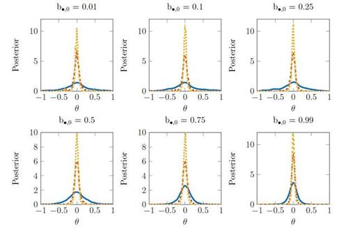
We now illustrate the behavior of the posterior $\widehat{\pi }(\theta ,\Gamma |S_n)$ under different levels of model misspecification in the running example. Following the analysis in Section 2.2, we consider three sample sizes n = 100, 500, 1000. The posterior is sampled using the robust option in the BSL package (An et al., 2022) under the default prior choice for Γ.¹⁰

We plot the robust posteriors in Figure 4. The results demonstrate that the robust posteriors for θ are Gaussian and concentrating around θ = 0, with the robust posterior seemingly being insensitive to the level of model misspecification. This behavior is due to the regularization of the covariance matrix, which ensures the criterion is globally concave and achieves its maximum at θ = 0. The results in Figure 4 provide convincing evidence that R-BSL yields reliable posteriors in a much broader set of circumstances than originally investigated in Frazier and Drovandi (2021), which considered the analysis of the R-BSL posterior in the MA(1) model but only considered a single misspecified DGP with sample size n = 100.

While Frazier and Drovandi (2021) prove posterior concentration of $\widehat{\pi }(\theta ,\Gamma |S_n)$ in the case of correctly specified models, as with the posterior $\widehat{\pi }(\theta |S_n)$, these arguments do not extend to the case of misspecified models. Determining the theoretical behavior of $\widehat{\pi }(\theta ,\Gamma |S_n)$ is significantly complicated by the introduction of Γ and the behavior of these components when the model is misspecified. While the authors have observed reliable behavior for $\widehat{\pi }(\theta ,\Gamma |S_n)$ across a multitude of examples, formal results on the asymptotic behavior of $\widehat{\pi }(\theta ,\Gamma |S_n)$ would require specific conditions on the prior $\pi (\Gamma )$, and the construction of novel arguments to deduce the asymptotic results. Given these complications, we leave a comprehensive study on the behavior of $\widehat{\pi }(\theta ,\Gamma |S_n)$ for future work.

4.2.2 A Robust Adjustment Approach

While the robust synthetic likelihood approach delivers reliable inference even in highly-misspecified models, it requires conducting posterior inference over $d_{\theta }+d$ (where $d\ge d_{\theta })$ elements, which can become cumbersome in cases where either θ or S_n is high-dimensional. However, the key insight of Frazier and Drovandi (2021) in regards to misspecification is that it can be handled by sufficiently altering the structure of the synthetic likelihood.

An alternative approach to deal with model misspecification in the case of high-dimensional summaries, or parameters, is to replace the covariance matrix ${\widehat{\Sigma }}_n(\theta )$ in $g_n(S_n|\theta )$ with a naive but fixed version A_n . Replacing ${\widehat{\Sigma }}_n(\theta )$ by the fixed matrix A_n means that $\hspace{0.17em}\log \hspace{0.17em}{g}_n(S_n|\theta )$ is roughly a weighted quadratic form based on a fixed covariance matrix, and thus should be well-behaved. As the result of Theorem 2 suggests, if this naive posterior is indeed uni-modal, then it will be approximately Gaussian in large samples, but with a covariance matrix that depends on the choice of A_n .

An unintended consequence of replacing ${\widehat{\Sigma }}_n(\theta )$ in $g_n(S_n|\theta )$ by the naive covariance matrix A_n is that the resulting posterior will concentrate onto values of θ under which $\left|\right|A_n^{-1/2}\{b(\theta )-S_n\}|{|}_{}$ is small. Therefore, such a procedure ensures that the specific choice of A_n influences the resulting pseudo-true value onto which the posterior will concentrate. To ensure that the pseudo-true value onto which the posterior concentrates remains meaningful, we suggest setting $A_n=I_d/n$, so that the naive posterior asymptotically concentrates onto the minimizer of $\left|\right|b(\theta )-b_{•}\left|\right|$. This choice ensures that the resulting pseudo-true value remains a meaningful quantity in approximate Bayesian inference.¹¹

While the naive posterior will concentrate onto a meaningful pseudo-true value, the coverage of the resulting posterior will not have the correct level (see Remark 8). However, we can adjust the posterior variance to ensure it attains the correct level of frequentist coverage. In particular, we can follow a similar idea to the adjustment procedure of Frazier et al. (2022) and adjust the posterior draws using the following algorithm.

1. Take ${\widehat{\Sigma }}_n(\theta )=A_n$, for all $\theta \in \Theta$, as the covariance matrix in the synthetic likelihood and obtain the corresponding naive posterior mean, ${\overline{\theta }}_n$, and posterior covariance, ${\widehat{\Delta }}_n$.

2. For θ^j , $j=1,\dots ,N$, a sample from the naive posterior, adjust θ^j according to ${\tilde{\theta }}^j={\overline{\theta }}_n+{\widehat{\Delta }}_n{\widehat{W}}_n^{1/2}{\widehat{\Delta }}_n^{-1/2}({\theta }^j-{\overline{\theta }}_n),$ where ${\widehat{W}}_n$ is any consistent estimator of the asymptotic variance $W_{\mathrm{\star }}:=\underset{n}{\lim }\text{var}\{\sqrt{n}{M}_n({\theta }_{\mathrm{\star }})\}$.

While the naive posterior in the first step ensures concentration onto values of θ under which $\left|\right|b(\theta )-b_{•}\left|\right|$ is small, this posterior has unreliable uncertainty quantification, and so the second step adjusts the posterior variance. When the model is misspecified, the most reliable estimator of $W_{\mathrm{\star }}:=\underset{n}{\lim }\text{var}\{\sqrt{n}{M}_n({\theta }_{\mathrm{\star }})\}$ is obtained using bootstrapping where we re-sample the summary statistics and recalculate the synthetic likelihood equations $M_n(\theta )$ at each bootstrapped summary statistic. In this way, we can interpret the above adjusted posterior as being similar to the “BayesBag” posterior (see Huggins and Miller, 2019), but in the synthetic likelihood context. However, unlike BayesBag our approach does not require re-running any posterior sampling mechanism, and only requires bootstrapping summary statistics and recalculating the synthetic likelihood score equations. Moreover, unlike BayesBag, the following result demonstrates that the adjusted posterior delivers asymptotically valid uncertainty quantification.

Let ${\theta }_n:=\arg {\min }_{\theta \in \Theta }\left|\right|b(\theta )-S_n\left|\right|,\vartheta :=\sqrt{n}(\tilde{\theta }-{\theta }_n)$, and ${\mathcal{T}}_n=\{t:\vartheta =\sqrt{n}(\tilde{\theta }-{\theta }_n),\tilde{\theta }\in \Theta \}$, where $\tilde{\theta }$ denotes the transformed version of θ given in the second step of the algorithm.

Corollary 3. Assume Assumptions 1, 2, and Assumptions 4-9 are satisfied, and that ${\widehat{\Delta }}_n$ and ${\widehat{W}}_n$ are consistent estimators for Δ and $W_{\mathrm{\star }}$, respectively. For $m\to \infty$ as $n\to \infty$, ${\int }_{{\mathcal{T}}_n}\left|\widehat{\pi }(\vartheta |S_n)-N\{\vartheta ;0,\Delta W_{\mathrm{\star }}{\Delta }^{\mathrm{\top }}\}\right|\mathrm{d}\vartheta =o_p(1)$, and for ${\tilde{\theta }}_n^{}:={\int }_{\Theta }\tilde{\theta }·\widehat{\pi }(\tilde{\theta }|S_n)\mathrm{d}\tilde{\theta }$, $\sqrt{n}({\tilde{\theta }}_n-{\theta }_{•})\Rightarrow N(0,{\Delta }^{}{W}_{\mathrm{\star }}{\Delta }^{\mathrm{\top }})$.

Remark 10. The adjusted BSL posterior concentrates onto the same limiting value as the ABC posterior under model misspecification. However, unlike the ABC posterior the adjusted BSL posterior displays Gaussian posterior concentration, and asymptotically correctly quantifies uncertainty about the pseudo-true value ${\theta }_{•}:=\arg {\min }_{\theta \in \Theta }\left|\right|b(\theta )-b_{•}\left|\right|$. Consequently, if the user is faced with a misspecified model in approximate Bayesian inference, and correct uncertainty quantification is desirable, then we recommend the use of robust BSL methods over ABC methods.

Remark 11. The above adjustment procedure is related to, but distinct from, the procedure discussed in Section 4 of Frazier et al. (2022). In correctly specified models, Frazier et al. (2022) use a similar approach to the second step of the above algorithm to correct the posterior covariance in cases where a computational convenient covariance matrix is initially used in BSL. We advise against using the approach outlined in Frazier et al. (2022) when the model is misspecified, since the resulting posterior will concentrate onto a point that is determined by the choice of computationally convenient covariance matrix. Due to space limitations, we forgo a detailed comparison with the adjustment approach of Frazier et al. (2022) to Appendix D.2.

We now examine the behavior of the adjusted posterior in the running example through a repeated sampling experiment. In particular, we generate five hundred datasets from the model in (2), where the parameter values are $\omega =-0.15,\rho =0.90$ and ${\sigma }_v=0.40$, and with n = 100, 500, 1000 observations. The adjusted posterior is obtained by calculating the exact naive posterior, setting A_n to be the identity covariance matrix, and then adjusting 10,000 samples from the naive posterior. The variance term ${\widehat{W}}_n$ used in the adjustment is estimated via the block bootstrap with a block size of 5 and using 1,000 bootstrap samples.

In Table 1 we record the posterior mean (multiplied by 10³), variance and Monte Carlo coverage for both the adjusted and naive approaches, and across each of the three samples sizes. The results demonstrate that both approaches give precise estimators for the location of the pseudo-true value, θ = 0, with the adjusted approach having a smaller posterior variance across all sample sizes. In terms of Monte Carlo coverage, both procedures display over-coverage for the unknown pseudo-true value. Therefore, given the tighter posteriors for the adjusted approach, and similar posterior means, we conclude that the adjusted approach is more accurate than the naive approach.

In Supplementary Appendix F we apply the robust procedures discussed in Section 4.2 to analyze a simple model of financial returns. Both methods behave similarly and suggest the presence of significant model misspecification.

5 Discussion

Over the last decade, approximate Bayesian methods like synthetic likelihood have gained acceptance in the statistical community for their ability to produce meaningful inferences in complex models. The ease with which these methods can be applied has also led to their use in diverse fields of research; see Sisson et al. (2018) for examples.

While the initial impetus for these methods was one of practicality, recent research has begun to focus on the theoretical behavior of these methods. In the context of BSL, Frazier et al. (2022) demonstrate that BSL posteriors are well-behaved in large samples, and can deliver inferences that are just as reliable as those obtained by ABC, assuming the model is correctly specified.

However, the important message delivered in this paper is that if the assumed model is misspecified, then synthetic likelihood-based inference can be unreliable, and the resulting posterior can be significantly different to those obtained from other approximate Bayesian methods. Critically, the type of behavior exhibited by the Bayesian synthetic likelihood posterior is intimately related to the form and degree of model misspecification, which cannot be reliably measured without first conducting some form of inference.

While our results have only focused on the most commonly applied variant of the synthetic likelihood posterior, we conjecture that recently proposed variations, such as the semiparametric approach of An et al. (2020) or the whitening approach of Priddle et al. (2021), will exhibit similar behavior. The semiparametric synthetic likelihood approach of An et al. (2020) allows the user to remove the implicit Gaussian assumption for the summary statistic likelihood and estimate the likelihood of the summaries using kernel smoothing methods. However, this more general approach will still suffer from the same issues as the original BSL posterior under model misspecification. Estimating the distribution of the summary statistics does not change the fact that when the model is misspecified the observed summary statistic cannot be matched by the simulated statistics. Consequently, changing the class of approximations used for the synthetic likelihood from the Gaussian to a more flexible class does not address the underlying issue of model misspecification, and so the resulting posterior will behave similarly to those analyzed herein.

Supplementary material. The supplementary material contains proofs of all technical results presented in the paper, additional numerical details and results, and an application of the adjustment procedures discussed in Section 4 to an empirical example on financial returns.

Acknowledgments. We are grateful to the Associate Editor and two referees for their very helpful comments and suggestions that have significantly improved the paper. All remaining errors are our own. Frazier and Drovandi were supported by Australian Research Council funding schemes DE200101070 and FT210100260, respectively. Nott was supported by a Singapore Ministry of Education Academic Research Fund Tier 1 grant.

Notes

¹ We later clarify that even the proof techniques used in Frazier et al. (2022) are not applicable in misspecified models, and that the posterior concentration results in Frazier and Drovandi (2021) do not extend to misspecified models.

² We note that the behavior observed in Figure 1 is in stark contrast to the findings in Frazier and Drovandi (2021), where the authors found that, under a different parameterization of the same model, at small sample sizes (n = 100) the BSL posterior placed most of its mass near the boundary of the parameter space.

³ The precise formulas are too long to state analytically. The interested reader is referred to the supplementary material where it is given in full detail.

⁴ We thank an anonymous referee for bringing this possible interpretation to our attention.

⁵ The behavior of the posterior when a root is on the boundary of the parameter space can be complicated, and so we leave a detailed study of this situation for future research.

⁶ Given Assumption 1, a sufficient condition for Assumption 4 is that $\theta \mapsto b(\theta )$ and $\theta \mapsto {\Sigma }_n(\theta )$ are twice continuously differentiable.

⁷ In the case of correctly specified models, Δ in Theorem 1 has the form $\Delta ={[{\{\partial b(\theta )/\partial {\theta }^{\mathrm{\top }}\}}^{\mathrm{\top }}\Sigma {(\theta )}^{-1}\{\partial b(\theta )/\partial {\theta }^{\mathrm{\top }}\}]}^{-1}$. However, when the model is misspecified this is not the case, and the general definition of Δ is given in Supplementary Appendix C.

⁸ The results displayed in Figure 3 are not overly sensitive to the choice of α.

⁹ For simplicity, we only focus on the variance adjustment approach detailed in Frazier and Drovandi (2021).

¹⁰ We start the sampler at θ = 0 and retain all resulting draws. In addition, we run the sampler for 50,000 iterations and use 10 synthetic datasets for each replication. These choices are fixed across the different sample size and misspecification combinations. The acceptance rates for the resulting procedure are reasonable, and between 20% and 60% across all combinations.

¹¹ Under the choice of $A_n=I_d/n$, the pseudo-true value onto which the posterior would concentrate would be ${\theta }_{•}:=\arg {\min }_{\theta \in \Theta }\left|\right|b(\theta )-b_{•}\left|\right|$, which can be interpreted as the value of $\theta \in \Theta$ that yields the closest match to the observed summaries in the Euclidean norm, and is the same value onto which the ABC posterior will concentrate if $\left|\right|·\left|\right|$ were used in ABC.

Table 1 Summary measures of posterior accuracy, calculated as averages across the replications. Mean - posterior mean multiplied by 10³, Variance - posterior variance, Coverage - Monte Carlo coverage. n-BSL refers to naive BSL, and a-BSL refers to adjusted BSL.

	n = 100		n = 500		n = 1,000
	a-BSL	n-BSL	a-BSL	n-BSL	a-BSL	n-BSL
Mean	−0.5691	−0.1955	−0.9916	0.0863	−0.2654	0.0191
Variance	0.0966	0.3322	0.0197	0.0668	0.0107	0.0334
Coverage	100%	100%	100%	100%	100%	100%

Figure 1 Bayesian synthetic likelihood posterior for θ in the misspecified moving average model.

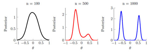
Figure 2 Comparison of the exact (synthetic likelihood) posterior under different levels of model misspecification. The solid line corresponds to n = 100, the dashed line to n = 500 and the dotted line to n = 1000.

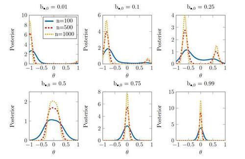
Figure 3 Tempered Bayesian synthetic likelihood posteriors for θ in the running example.

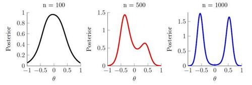
Figure 4 r-BSL Posteriors for θ in the misspecified MA(1) model across six different levels of model misspecification. The solid line corresponds to n = 100, the dashed line to n = 500 and the dotted line to n = 1000.