Dualization and Automatic Distributed Parameter Selection of Total Generalized Variation via Bilevel Optimization

Abstract

Total Generalized Variation (TGV) regularization in image reconstruction relies on an infimal convolution type combination of generalized first- and second-order derivatives. This helps to avoid the staircasing effect of Total Variation (TV) regularization, while still preserving sharp contrasts in images. The associated regularization effect crucially hinges on two parameters whose proper adjustment represents a challenging task. In this work, a bilevel optimization framework with a suitable statistics-based upper level objective is proposed in order to automatically select these parameters. The framework allows for spatially varying parameters, thus enabling better recovery in high-detail image areas. A rigorous dualization framework is established, and for the numerical solution, a Newton type method for the solution of the lower level problem, i.e. the image reconstruction problem, and a bilevel TGV algorithm are introduced. Denoising tests confirm that automatically selected distributed regularization parameters lead in general to improved reconstructions when compared to results for scalar parameters.

Keywords:

• Image denoising
• regularization parameter selection
• bilevel optimization
• total generalized variation

1. Introduction

In this work we analyze and implement a bilevel optimization framework for automatically selecting spatially varying regularization parameters $\mathit{\alpha }:=({\alpha }_0,{\alpha }_1)\in C{(\overline{\Omega })}^2,\mathit{\alpha }>0,$ in the following image reconstruction problem: (1.1) $$\text{minimize}\hspace{1em}\frac{1}{2}{\int }_{\Omega }{(Tu-f)}^{2}dx+{\text{TGV}}_{\mathit{\alpha }}^2(u)\hspace{1em}\text{over}\mathrm{ }u\in \text{BV}(\Omega ),$$(1.1) where the second-order Total Generalized Variation (TGV) regularization is given by (1.2) $$\begin{array}{c}{\text{TGV}}_{\mathit{\alpha }}^2(u)=\sup \{{\int }_{\Omega }u {\text{div}}^2\varphi dx:\varphi \in C_c^{\infty }(\Omega ,{\mathcal{S}}^{d\times d}),|\varphi (x)|\le {\alpha }_0(x),\hfill \\ |\text{div}\varphi (x)|\le {\alpha }_1(x),\mathrm{ }\text{for}\mathrm{ }\text{all}\mathrm{ }x\in \Omega \}.\hfill \end{array}$$(1.2)

Here, $\Omega \subseteq {\mathbb{R}}^d$ is a bounded, open image domain with Lipschitz boundary, ${\mathcal{S}}^{d\times d}$ denotes the space of d × d symmetric matrices, $T:L^2(\Omega )\to L^2(\Omega )$ is a bounded linear (output) operator, and f denotes given data which satisfies (1.3) $$f=T{u}_{\mathit{true}}+\eta .$$(1.3)

In this context, η models a highly oscillatory (random) component with zero mean and known quadratic deviation (variance) ${\sigma }^2$ from the mean. Further, $L^2(\Omega )$ denotes the standard Lebesgue space [1], and $|·|,$ represents the Euclidean vector norm or its associated matrix norm. The space of infinitely differentiable functions with compact support in $\Omega$ and values in ${\mathcal{S}}^{d\times d}$ is denoted by $C_c^{\infty }(\Omega ,{\mathcal{S}}^{d\times d}).$ Further, we refer to Section 2 for the definition of the first- and second-order divergences $\mathrm{div}$ and ${\mathrm{div}}^2,$ respectively.

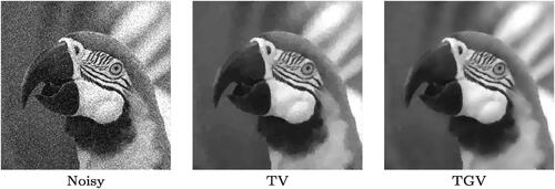
Originally, the TGV functional was introduced for scalar parameters ${\alpha }_0,{\alpha }_1>0$ only; see [2]. It serves as a higher order extension of the well-known Total Variation (TV) regularizer [3,4], preserves edges (i.e., sharp contrast) [5,6], and promotes piecewise affine reconstructions while avoiding the often adverse staircasing effect (i.e., piecewise constant structures) of TV [7–9]; see Figure 1 for an illustration. These properties of TGV have made it a successful regularizer in variational image restoration for a variety of applications [2, 10–16]. Extensions to manifold-valued data, multimodal and dynamic problems [17–22] have been proposed as well. In all of these works, the choice of the scalar parameters ${\alpha }_0,{\alpha }_1$ is made “manually” via a direct grid search. Alternatively, selection schemes relying on a known ground truth u_true have been studied; see [23–26]. The latter approach, however, is primarily of interest when investigating the mere capabilities of TGV regularization.

Figure 1. Gaussian denoising: Typical difference between TV (piecewise constant) and TGV reconstructions (piecewise affine).

While there exist automated parameter choice rules for TV regularization, see for instance [27] and the references therein, analogous techniques and results for the TGV parameters are very scarce. One of the very few contributions is [28] where, however, a spatially varying fidelity weight rather then regularization parameter is computed. Compared to the choice of the regularization weight in TV-based models, the infimal convolution type regularization incorporated into the TGV functional significantly complicates the selection; compare the equivalent definition (2.1) below. Further difficulties arise when these parameters are spatially varying as in (1.2). In that case, by appropriately choosing $\mathit{\alpha }=({\alpha }_0,{\alpha }_1),$ one wishes to smoothen homogeneous areas in the image while preserving fine scale details. The overall target is then to not only select the parameters in order to reduce noise while avoiding oversmoothing, as in the TV case, but also to ensure that the interplay of α₀ and α₁ will not produce any staircasing.

For this delicate selection task and inspired by [27, 29] for TV, in this work we propose a bilevel minimization framework for an automated selection of $\mathit{\alpha }$ in the TGV case. Formally, the setting can be characterized as follows: (1.4) $$\{\begin{array}{c}\mathit{minimize}\text{ a }\text{statistics}-\text{based}\mathrm{ }\mathrm{(}\text{upper}\mathrm{ }\text{level}\mathrm{)}\mathrm{ }\text{objective}\mathrm{ }\text{over}\mathrm{ }(u,\mathit{\alpha })\hfill \\ \mathit{subject}tou\text{solving}(1.1)\text{for a regularization weight}\mathit{\alpha }=({\alpha }_0,{\alpha }_1).\hfill \end{array}$$(1.4)

Note here that the optimization variable $\mathit{\alpha }$ enters the lower level minimization problem (1.1) as a parameter, thus giving rise to $u=u(\mathit{\alpha }).$ We also mention that this optimization format falls into the general framework which is discussed in our review paper [30] where the general opportunities and mathematical as well as algorithmic aspects of bilevel optimization in generating structured non-smooth regularization functionals are discussed in detail.

As our statistical set-up parallels the one in [27, 29], here we resort to the upper level objective proposed in that work. It is based on localized residuals $\mathrm{R}:L^2(\Omega )\to L^{\infty }(\Omega )$ with (1.5) $$\mathrm{R}u(x)={\int }_{\Omega }w(x,y){(Tu-f)}^2(y) dy,$$(1.5) where $w\in L^{\infty }(\Omega \times \Omega )$ with ${\int }_{\Omega }{\int }_{\Omega }w(x,y)\mathit{dxdy}=1.$ Note that $\mathrm{R}u(x)$ can be interpreted as a local variance keeping in mind that, assuming Gaussian noise of variance ${\sigma }^2,$ we have that ${\int }_{\Omega }{(T{u}_{\mathit{true}}-f)}^2 dx={\int }_{\Omega }{\eta }^2 dx={\sigma }^2\left|\Omega \right|.$ Consequently, if a reconstructed image u is close to u_true then it is expected that for every $x\in \Omega$ the value of $\mathrm{R}u(x)$ will be close to ${\sigma }^2.$ Hence it is natural to consider an upper level objective which aims to approximately keep $\mathrm{R}u$ within a corridor ${\underset{¯}{\sigma }}^2\le {\sigma }^2\le {\overline{\sigma }}^2$ with positive bounds ${\underset{¯}{\sigma }}^2,{\overline{\sigma }}^2.$ This can be achieved by utilizing the function $F:L^2(\Omega )\to \mathbb{R}$ with (1.6) $$F(v):=\frac{1}{2}{\int }_{\Omega }\max {(v-{\overline{\sigma }}^2,0)}^{2}dx+\frac{1}{2}{\int }_{\Omega }\min {(v-{\underset{¯}{\sigma }}^2,0)}^{2}dx.$$(1.6)

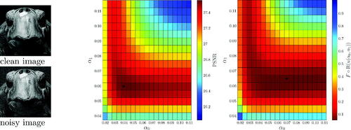
The function $F(\mathrm{R}·)$ is then indeed suitable as an upper level objective. This is demonstrated in Figure 2, where we show (in the middle and right plots) the objective values for a series of scalar TGV denoising results and for a variety of parameters $({\alpha }_0,{\alpha }_1)$ for the image depicted on the left. Regarding the choices of $\underset{¯}{\sigma },\overline{\sigma },w$ we refer to Section 5. Upon inspection of Figure 2 we find that the functional $F(\mathrm{R}·)$ is minimized for a pair of scalar parameters $({\alpha }_0,{\alpha }_1)$ that is close to the one maximizing the peak-signal-to-noise-ratio (PSNR). Note, however, that in order to truly optimize the PSNR, one would need the ground truth image u_true, which is of course typically not available. In contrast to this, we emphasize that $F(\mathrm{R}·)$ does not involve any ground truth information. Rather, it only relies on statistical properties of the noise.

Figure 2. Suitability of the functional $F(\mathrm{R}·)$ as an upper level objective. Evaluation of $F(\mathrm{R}u)$ where u solves the TGV denoising problem (1.1) (T = Id), for a variety of scalar parameters $({\alpha }_0,{\alpha }_1).$

For analytical and numerical reasons, rather than having (1.1) as the lower level problem for the bilevel minimization framework (1.4), one can use alternative formulations, as was done for instance in [27, 29] for TV models, where the Fenchel predual problem was used instead, see also [30] for a thorough discussion on the corresponding TGV model. This yields a bilevel problem which is expressed in terms of dual variables and is equivalent to the one stated in terms of the primal variable u. In this way, one has to treat a more amenable variational inequality of the first kind rather than one of second kind in the primal setting in the constraint system of the resulting bilevel optimization problem. Numerically, one may then utilize very efficient and resolution independent, function space based solution algorithms, like (inexact) semismooth Newton methods [31]. The other option that we will consider in this work, is to minimize the upper level objective subject to the primal-dual optimality conditions, for which Newton methods can also be applied for their solution, see for instance [32] for an inexact semismooth Newton solver which operates on the primal-dual optimality conditions for TV regularization. We should also mention that this approach requires $T^{\ast }T$ to be invertible, with $T^{\ast }$ being the adjoint of T, which is true when T is injective with closed range. We note that this does not exclude the use of our bilevel scheme to inverse problems whose forward operator does not satisfy this condition. A noninvertibility of $T^{\ast }T$ can for instance be treated by adding a small regularization term of the form $\frac{\kappa }{2}{\int }_{\Omega }{u}^2 dx,$ in combination with a Levenberg-Marquardt algorithmic scheme that sends the parameter κ to zero along the iterations. Alternatively, instead of Newton, one can resort to first-order methods for solving the lower level problem for which invertibility of $T^{\ast }T$ is not required. Such approaches are definitely interesting and necessary for many inverse problems however since they would deviate from the main focus of our paper which is the automatic computation of spatially distributed regularization weights, we will keep this invertibility assumption in the following.

2. The structure of the paper

Basic facts on the TGV functional with spatially varying parameters along with functional analytic foundations needed for (pre)dualization are the subjects of Section 2. Section 2.4 is concerned with the derivation of the predual problem of (1.1) and the corresponding primal-dual optimality conditions. Regularized versions of these conditions are the focus of Section 3. Besides respective primal-dual optimality conditions, we study the asymptotic behavior of these problems and their associated solutions under vanishing regularization. Section 4 introduces the bilevel TGV problem for which the primal-dual optimality conditions serve as constraints. The numerical solution of the proposed bilevel problem is the subject of Section 5. It is also argued that every regularized instance of the lower level problem can be solved efficiently by employing an (inexact) semismooth Newton method. The paper ends by a report on extensive numerical tests along with conclusions drawn from these computational results.

Summarizing, this work provides not only a user-friendly and novel hierarchical variational framework for automatic selection of the TGV regularization parameters, but by making these parameters spatially dependent it leads to an overall performance improvement; compare, e.g., the results in Section 5.

3. The dual form of the weighted TGV functional

3.1. Total generalized variation

We recall here some basic facts about the TGV functional (1.2) with constant parameters ${\alpha }_0,{\alpha }_1$ and assume throughout that the reader is familiar with the basic concepts of functions of bounded variation (BV); see [33] for a detailed account. For a function $\varphi \in C_c^{\infty }(\Omega ,{\mathcal{S}}^{d\times d})$ the first- and second-order divergences are, respectively, given by $${(\text{div}\varphi )}_i=\sum _{j=1}^d\frac{\partial {\varphi }_{ij}}{\partial x_j},i=1,\dots ,d,\hspace{1em}\text{and}\hspace{1em}{\text{div}}^2\varphi =\sum _{i=1}^d\frac{{\partial }^2{\varphi }_{ii}}{\partial x_i^2}+2\sum _{i<j}\frac{{\partial }^2{\varphi }_{ij}}{\partial x_i\partial x_j}.$$

In [14] it was shown that a function $u\in L^1(\Omega )$ has finite $\text{TGV}$ value if and only if it belongs to $\text{BV}(\Omega ).$ Here $\text{BV}(\Omega )$ denotes the Banach space of function of bounded variation over $\Omega$ with associated norm $\Vert ·{\Vert }_{\text{BV}(\Omega )}.$ Moreover, the bounded generalized variation norm $\Vert ·{\Vert }_{\text{BGV}}:=\Vert ·{\Vert }_{L^1(\Omega )}+{\text{TGV}}_{\mathit{\alpha }}^2(·)$ is equivalent to $\Vert ·{\Vert }_{\text{BV}(\Omega )}.$ Similarly to TV, TGV is a convex functional which is lower semicontinuous with respect to the strong L¹ convergence. In [14, 34] it is demonstrated that the TGV functional can be equivalently written as (2.1) $${\text{TGV}}_{\mathit{\alpha }}^2(u)=\underset{w\in \text{BD}(\Omega )}{\min }{\alpha }_1|Du-w|(\Omega )+{\alpha }_0\left|\mathcal{E}w\right|(\Omega ),$$(2.1) where $\text{BD}(\Omega )$ is the Banach space of functions of bounded deformation, with $\mathcal{E}$ denoting the distributional symmetrized gradient [35,36]. The asymptotical behavior of the TGV model in image restoration with respect to scalars ${\alpha }_0,{\alpha }_1$ was studied in [37]; see also [6]. For instance, when T = Id and either α₀ or α₁ converges to zero, then the corresponding solutions of (1.1) converge (weakly${}^{\ast }$ in $\text{BV}(\Omega )$) to f. When both of the parameters are sent to infinity, then the solutions converge weakly${}^{\ast }$ to the L²-linear regression solution for f. We further note that the set of affine functions constitutes the kernel of the TGV functional.

For specific symmetric functions u, there exist combinations of ${\alpha }_0,{\alpha }_1$ such that ${\text{TGV}}_{\mathit{\alpha }}(u)={\alpha }_1\text{TV}(u).$ In general one can show that there exists a constant C > 0 such that if ${\alpha }_0/{\alpha }_1>C,$ then the $\text{TGV}$ value does not depend on α₀ and, up to an affine correction, it is equivalent to $\text{TV}.$ In that case the reconstructed images still suffer from a kind of (affine) staircasing effect [37].

The fine structure of TGV reconstructions has been studied analytically mainly in dimension one in [5, 38–41]. Under some additional regularity assumptions (compare [6]) it can be shown that for TGV denoising the jump set of the solution is essentially contained in the jump set of the data; see [42] for the TV case.

3.2. The space $W_0^q({\text{div}}^2;\Omega )$

Next we introduce several function spaces which will be useful in our subsequent development. For this purpose, let $1\le q\le \infty$ and $p\in L^q(\Omega ,{\mathbb{R}}^d).$ Recall that $\text{div}p\in L^q(\Omega )$ if there exists $w\in L^q(\Omega )$ such that $${\int }_{\Omega }\nabla \varphi ·p dx=-{\int }_{\Omega }\varphi w dx,\hspace{1em}\text{for}\mathrm{ }\text{all}\mathrm{ }\varphi \in C_c^{\infty }(\Omega ).$$

In that case w is unique and we set $\text{div}p=w.$ Based on this first-order divergence, we define the Banach space $$W^q(\text{div};\Omega ):=\left\{p\in L^q(\Omega ,{\mathbb{R}}^d):\text{div}p\in L^q(\Omega )\right\},$$ endowed with the norm $\Vert p{\Vert }_{W^q(\text{div};\Omega )}^q:=\Vert p{\Vert }_{L^q(\Omega ,{\mathbb{R}}^d)}^q+\Vert \text{div}p{\Vert }_{L^q(\Omega )}^q.$ Similarly one obtains the Banach space $W^q({\text{div}}^2;\Omega )$ as the space of all functions $p\in L^q(\Omega ,{\mathcal{S}}^{d\times d})$ whose first- and second-order divergences, $\text{div}p$ and ${\text{div}}^{2}p,$ respectively, belong to $L^q(\Omega ).$ We note that for a $p\in L^q(\Omega ,{\mathcal{S}}^{d\times d}),$ we have that $\text{div}p\in L^q(\Omega ,{\mathbb{R}}^d)$ if there exists an $\omega \in L^q(\Omega ,{\mathbb{R}}^d)$ such that $${\int }_{\Omega }E\varphi ·p dx=-{\int }_{\Omega }\varphi ·\omega dx,\hspace{1em}\text{for}\mathrm{ }\text{all}\mathrm{ }\varphi \in C_c^{\infty }(\Omega ,{\mathbb{R}}^d),$$ with $E\varphi$ denoting the L¹ function representing the absolutely continuous part of $\mathcal{E}\varphi ,$ with respect to the Lebesgue measure. Note that since $\varphi$ is smooth, we have $\mathcal{E}\varphi =E\varphi .$ As before ω is unique and we set $\text{div}p=\omega .$ Finally ${\text{div}}^{2}p\in L^q(\Omega )$ if there exists a function $v\in L^q(\Omega )$ such that $${\int }_{\Omega }\nabla \varphi ·\text{div}p dx=-{\int }_{\Omega }\varphi v dx,\hspace{1em}\text{for}\mathrm{ }\text{all}\mathrm{ }\varphi \in C_c^{\infty }(\Omega ).$$

This space is equipped with the norm $\Vert p{\Vert }_{W^q({\text{div}}^2;\Omega )}^q:=\Vert p{\Vert }_{L^q(\Omega )}^q+\Vert \text{div}p{\Vert }_{L^q(\Omega ,{\mathbb{R}}^d)}^q+\Vert {\text{div}}^{2}p{\Vert }_{L^q(\Omega )}^q.$ We refer to [12] for a more general definition of these spaces. Note that when q = 2 these spaces are Hilbertian and then the standard notation is $H(\text{div};\Omega )$ and $H({\text{div}}^2;\Omega );$ see [43]. The Banach spaces $W_0^q(\text{div};\Omega )$ and $W_0^q({\text{div}}^2;\Omega )$ are defined as $$W_0^q(\text{div};\Omega )={\overline{C_c^{\infty }(\Omega ,{\mathbb{R}}^d)}}^{\Vert ·{\Vert }_{W^q(\text{div};\Omega )}},\mathrm{\hspace{1em}}\mathrm{\hspace{1em}}{W}_0^q({\text{div}}^2;\Omega )={\overline{C_c^{\infty }(\Omega ,{\mathcal{S}}^{d\times d})}}^{\Vert ·{\Vert }_{W^q({\text{div}}^2;\Omega )}},$$ with the analogous notation $H_0(\text{div};\Omega )$ and $H_0({\text{div}}^2;\Omega )$ for q = 2. Using the definitions above, the following integration by parts formulae hold true: (2.2) $${\int }_{\Omega }\nabla \varphi ·p dx=-{\int }_{\Omega }\varphi \text{div}p dx,\hspace{1em}\text{for}\mathrm{ }\text{all}\mathrm{ }p\in W_0^q(\text{div};\Omega ),\varphi \in C^{\infty }(\overline{\Omega },\mathbb{R}),$$(2.2) (2.3) $${\int }_{\Omega }E\varphi ·p dx=-{\int }_{\Omega }\varphi · \text{div}p dx,\hspace{1em}\text{for}\mathrm{ }\text{all}\mathrm{ }p\in W_0^q({\text{div}}^2;\Omega ),\varphi \in C^{\infty }(\overline{\Omega },{\mathbb{R}}^d),$$(2.3) (2.4) $${\int }_{\Omega }\nabla \varphi ·\text{div}p dx=-{\int }_{\Omega }\varphi {\text{div}}^{2}p dx,\hspace{1em}\text{for}\mathrm{ }\text{all}\mathrm{ }p\in W_0^q({\text{div}}^2;\Omega ),\varphi \in C^{\infty }(\overline{\Omega },\mathbb{R}).$$(2.4)

3.3. Weighted TGV

Throughout the remainder of this work we use the weighted TGV functional (1.2) with ${\alpha }_0,{\alpha }_1\in C(\overline{\Omega })$ and ${\alpha }_0(x),{\alpha }_1(x)>\underset{¯}{\alpha }>0,$ $\underset{¯}{\alpha }\in \mathbb{R},x\in \Omega .$ We denote by $|·|$ the finite dimensional Euclidean norm. We note that for an ${\mathbb{R}}^{\mathcal{\ell }}$-valued finite Radon measure $\mu =(m_1,\dots ,m_{\mathcal{\ell }}),$ we denote by $\left|\mu \right|$ its total variation measure, where for every Borel $E\subseteq \Omega$ $$\left|\mu \right|(E)=\sup \left\{\sum _{n=0}^{\infty }|\mu (E_n)|:E_n\mathrm{ }\text{Borel}\mathrm{ }\text{pairwise}\mathrm{ }\text{disjoint},\mathrm{ }E=\underset{n=0}{\overset{\infty }{\cup }}{E}_n\right\}.$$

Note also that it can be shown $$\left|\mu \right|(\Omega )=\sup \left\{\sum _{i=1}^{\mathcal{\ell }}{\int }_{\Omega }{\varphi }_i d{\mu }_i:\varphi \in C_c^{\infty }(\Omega ,{\mathbb{R}}^{\mathcal{\ell }}),|\varphi (x)|\le 1,\mathrm{ }\text{for}\mathrm{ }\text{all}\mathrm{ }x\in \Omega \right\}.$$

We will show that for $u\in L^2(\Omega )$ the space $C_c^{\infty }(\Omega ,{\mathcal{S}}^{d\times d})$ in (1.2) can be substituted by $H_0({\text{div}}^2;\Omega )$ (and by $W_0^d({\text{div}}^2;\Omega )$ for $u\in L^{d/d-1}(\Omega )$). This fact will be instrumental when deriving the predual of the TGV minimization problem. For this we need the following result:

Proposition 2.1.

The weighted ${\text{TGV}}_{\mathit{\alpha }}^2$ functional (1.2) admits the equivalent expression (2.5) $${\text{TGV}}_{\mathit{\alpha }}^2(u)=\underset{w\in \text{BD}(\Omega )}{\min }{\int }_{\Omega }{\alpha }_1 d|Du-w|+{\int }_{\Omega }{\alpha }_0 d\left|\mathcal{E}w\right|.$$(2.5)

Proof.

The proof is analogous to the one for the scalar TGV functional; see for instance [34, Theorem 3.5] or [12, Proposition 2.8]. Here, we highlight only the significant steps. Indeed, given $u\in L^1(\Omega ),$ the idea is to define $$\begin{array}{c}U=C_0^1(\Omega ,{\mathbb{R}}^d)\times C_0^2(\Omega ;{\mathcal{S}}^{d\times d}),\hspace{1em}V=C_0^1(\Omega ,{\mathbb{R}}^d),\\ \Lambda :U\to V,\hspace{1em}\Lambda (u_1,u_2)=-u_1-\text{div}{u}_2,\\ F_1:U\to \overline{\mathbb{R}},\hspace{1em}{F}_1(u_1,u_2)=-{\int }_{\Omega }u \text{div}{u}_1+{\mathcal{I}}_{\left\{\right|·(x)|\le {\alpha }_1(x)\}}(u_1)+{\mathcal{I}}_{\left\{\right|·(x)|\le {\alpha }_0(x)\}}(u_2),\\ F_2:V\to \overline{\mathbb{R}},\hspace{1em}{F}_2(v)={\mathcal{I}}_{\left\{0\right\}}(v).\end{array}$$

Here, ${\mathcal{I}}_S(·)$ denotes the indicator function of a set S. Now, after realizing that (2.6) $${\text{TGV}}_{\mathit{\alpha }}^2(u)=\underset{(u_1,u_2)\in U}{\sup }-F_1(u_1,u_2)-F_2(\Lambda (u_1,u_2)),$$(2.6) the proof proceeds by showing that the dual problem of (2.6) is equivalent to (2.5) and then applying the Fenchel duality result [44]. We note that in order to achieve zero duality gap between the primal and the dual problem the so-called Attouch-Brezis condition needs to be satisfied see [45], that is one needs to show that the set $\underset{\lambda \ge 0}{\cup }\lambda (\text{dom}(F_2)-\Lambda (\text{dom}(F_1)))$ is a closed subspace of V. Indeed one can easily see that $$\begin{array}{c}\underset{\lambda \ge 0}{\cup }\lambda (\text{dom}(F_2)-\Lambda (\text{dom}(F_1)))=\{\lambda (u_1+\text{div}{u}_2):(u_1,u_2)\in U,\\ \mathrm{\hspace{1em}}\mathrm{\hspace{1em}}|u_1(x)|\le {\alpha }_1(x),|u_2(x)|\le {\alpha }_0(x),\forall x\in \Omega \}=V.\end{array}$$

Note that for the above equality we crucially used the fact that α₁ is bounded away from zero.

The other subtle point is the following density result which is required in order to show that (2.6) is indeed equal to (1.2): (2.7) $$\begin{array}{cc}\hfill & {\overline{\left\{\varphi \in C_c^{\infty }(\Omega ,{\mathcal{S}}^{d\times d}):|\varphi (x)|\le {\alpha }_0(x),|\text{div}\varphi (x)|\le {\alpha }_1(x),\mathrm{ }\text{for}\mathrm{ }\text{all}\mathrm{ }x\in \Omega \right\}}}^{\Vert ·{\Vert }_{C_0^2}}\hfill \\ \hfill & =\left\{\psi \in C_0^2(\Omega ,{\mathcal{S}}^{d\times d}):|\psi (x)|\le {\alpha }_0(x),|\text{div}\psi (x)|\le {\alpha }_1(x),\mathrm{ }\text{for}\mathrm{ }\text{all}\mathrm{ }x\in \Omega \right\}.\hfill \end{array}$$(2.7)

Indeed let ψ belong to the second set in (2.7), and let $ϵ>0.$ Choose $0<{\lambda }_{ϵ}<1$ such that (2.8) $$\Vert \psi -{\lambda }_{ϵ}\psi {\Vert }_{C_0^2}<ϵ/2.$$(2.8)

Since α₀ and α₁ are continuous and bounded away from zero there exists ${\alpha }_{ϵ}>0,$ smaller than the minimum of ${\alpha }_0,{\alpha }_1,$ such that $$|{\lambda }_{ϵ}\psi (x)|\le {\alpha }_0(x)-{\alpha }_{ϵ},\hspace{1em}|\text{div}{\lambda }_{ϵ}\psi (x)|\le {\alpha }_1(x)-{\alpha }_{ϵ},\hspace{1em}\mathrm{ }\text{for}\mathrm{ }\text{all}\mathrm{ }x\in \Omega .$$

From standard density properties there exists a function ${\varphi }_{ϵ}\in C_c^{\infty }(\Omega ,{\mathcal{S}}^{d\times d})$ such that the following conditions hold for all $x\in \Omega :$ (2.9) $$\Vert {\varphi }_{ϵ}-{\lambda }_{ϵ}\psi {\Vert }_{C_0^2}<ϵ/2,\hspace{1em}|{\varphi }_{ϵ}(x)-{\lambda }_{ϵ}\psi (x)|\le {\alpha }_{ϵ}/2,\hspace{1em}|\text{div}{\varphi }_{ϵ}(x)-\text{div}{\lambda }_{ϵ}\psi (x)|\le {\alpha }_{ϵ}/2,$$(2.9) which implies (2.10) $$|{\varphi }_{ϵ}(x)|\le {\alpha }_0(x)-{\alpha }_{ϵ}/2,\hspace{1em}|\text{div}{\varphi }_{ϵ}(x)|\le {\alpha }_1(x)-{\alpha }_{ϵ}/2,\hspace{1em}\mathrm{ }\text{for}\mathrm{ }\text{all}\mathrm{ }x\in \Omega .$$(2.10)

Then, from (2.10) it follows that ${\varphi }_{ϵ}$ belongs to the first set in (2.7) and from (2.8) and (2.9) we get that $\Vert \psi -{\varphi }_{ϵ}{\Vert }_{C_0^2}<ϵ.$ □

Now we are ready to establish the density result needed for dualization. For the sake of the flow of presentation we defer the proof, which parallels the one of [12, Proposition 3.3], to Appendix A. Below “a.e.” stands for “almost every” with respect to the Lebesgue measure.

Proposition 2.2.

For $u\in L^2(\Omega )$, the weighted TGV functional (1.2) can be equivalently written as (2.11) $$\begin{array}{cc}{\text{TGV}}_{\mathit{\alpha }}^2(u)=\sup \{{\int }_{\Omega }u {\text{div}}^{2}p dx:p\in H_0({\text{div}}^2;\Omega ),\hfill & |p(x)|\le {\alpha }_0(x),\hfill \\ \hfill & |\text{div}p(x)|\le {\alpha }_1(x),\mathit{\text{fora}}.\mathit{e}.\mathit{x}\in \Omega \}.\hfill \end{array}$$(2.11)

Remark:

By slightly amending the proof of Proposition 2.2, one can also show that if $u\in L^{d/d-1}(\Omega )\supset \text{BV}(\Omega )$ then the dual variables p can be taken to belong to $W_0^d({\text{div}}^2;\Omega )$ rather than $H_0({\text{div}}^2;\Omega ).$

3.4. The predual weighted TGV problem

Now we study the predual problem for the weighted TGV model with continuous weights, i.e., we use the regularization functional (1.2) or equivalently (2.11). For $T\in \mathcal{L}(L^2(\Omega ),L^2(\Omega ))$ we assume that $\mathcal{B}:=T^{\ast }T$ is invertible and define $\Vert v{\Vert }_{\mathcal{B}}^2={\int }_{\Omega }v{\mathcal{B}}^{-1}v,$ which induces a norm in $L^2(\Omega )$ equivalent to the standard one; compare [31]. When $T^{\ast }T$ is not invertible one can add an extra regularization term of the form $\frac{\kappa }{2}{\int }_{\Omega }{u}^2 dx,$ for some small $\kappa >0,$ to the objective in (1.1). Then $\mathcal{B}=\kappa \mathrm{Id}+T^{\ast }T$ will be invertible, see a similar approach in [27, 29, 31]. We mention that a different set-up, as adopted for instance in [46], assumes $T\in \mathcal{L}(L^{d/d-1},L^2(\Omega )),$ since $\text{BV}(\Omega )$ continuously embeds to $L^{d/d-1}(\Omega ).$ Then one readily finds that for d > 2, $\mathcal{B}$ cannot be invertible, in general. Even though invertibility of $T^{\ast }T$ is not necessary when dealing only with the TGV regularization problem (1.1), additional challenges would arise in our overall bilevel optimization context, such as, e.g., a lack of uniqueness of the solution for the lower level problem, i.e., genuine set-valuedness of the regularization-weight-to-reconstruction map cf. the constraint set in (1.4). In the next proposition we prove zero duality gap for (1.1) and its predual. We note however that the invertibility assumption on $T^{\ast }T$ is not needed to establish zero duality gap but rather to get an explicit formulation of the predual problem. An adaptation of the following proposition without this invertibility assumption can be done for instance by simply adjusting the corresponding proof of [46, Theorem 5.4] where analogous dualization results for a class of structural TV regularizers were considered.

Proposition 2.3.

Let $f\in L^2(\Omega )$, then there exists a solution to the primal problem (2.12) $$\mathit{\text{minimize}}\hspace{1em}\frac{1}{2}\Vert Tu-f{\Vert }_{L^2(\Omega )}^2+{\text{TGV}}_{\mathit{\alpha }}^2(u)\hspace{1em}\mathit{\text{over}}\mathrm{ }u\in \text{BV}(\Omega ),$$(2.12) as well as to its predual problem (2.13) $$\begin{array}{cc}\hfill & \mathit{\text{minimize}}\hspace{1em}\frac{1}{2}\Vert T^{\ast }f-{\text{div}}^{2}p{\Vert }_{\mathcal{B}}^2-\frac{1}{2}\Vert f{\Vert }_{L^2}^2\hspace{1em}\mathit{\text{over}}\mathrm{ }p\in H_0({\text{div}}^2;\Omega )\hfill \\ \hfill & \mathit{\text{subject}}\mathrm{ }\text{to}\hspace{1em}|p(x)|\le {\alpha }_0(x),|\text{div}p(x)|\le {\alpha }_1(x),\mathit{\text{fora}}.\mathit{e}.\mathit{x}\in \Omega ,\hfill \end{array}$$(2.13) and there is no duality gap, i.e., the primal and predual optimal objective values are equal. Moreover, the solutions u and p of these problems satisfy (2.14) $$\mathcal{B}u=T^{\ast }f-{\text{div}}^{2}p.$$(2.14)

Proof.

We set $U=H_0({\text{div}}^2;\Omega ),V=L^2(\Omega ),$ $\Lambda :U\to V$ with $\Lambda p={\text{div}}^{2}p,$ and also $F_1:U\to \overline{\mathbb{R}}$ and $F_2:V\to \overline{\mathbb{R}}$ with (2.15) $$F_1(p)={\mathcal{I}}_{\left\{\right|·(x)|\le {\alpha }_0(x),\text{fora}.\mathrm{e}.\mathrm{x}\}}(p)+{\mathcal{I}}_{\left\{\right|\text{div}·(x)|\le {\alpha }_1(x),\text{fora}.\mathrm{e}.\mathrm{x}\}}(p),$$(2.15) (2.16) $$F_2(\psi )=\frac{1}{2}\Vert T^{\ast }f-\psi {\Vert }_{\mathcal{B}}^2-\frac{1}{2}\Vert f{\Vert }_{L^2(\Omega )}^2.$$(2.16)

Immediately one gets that (2.17) $$\underset{p\in U}{\inf }{F}_1(p)+F_2(\Lambda p)=\underset{\begin{array}{c}p\in H_0({\text{div}}^2;\Omega )\\ |p(x)|\le {\alpha }_0(x)\\ |\text{div}p(x)|\le {\alpha }_1(x)\end{array}}{\min }\frac{1}{2}\Vert T^{\ast }f-{\text{div}}^{2}p{\Vert }_{\mathcal{B}}^2-\frac{1}{2}\Vert f{\Vert }_{L^2(\Omega )}^2.$$(2.17)

The problem in (2.17) admits a solution. Indeed, first observe that the objective is bounded from below. Then note that since $\frac{1}{2}\Vert T·-f{\Vert }_{L^2(\Omega )}^2$ is continuous at $0\in L^2(\Omega ),$ its convex conjugate (see [44] for a general definition) which is equal to $\frac{1}{2}\Vert T^{\ast }f+·{\Vert }_{\mathcal{B}}^2-\frac{1}{2}\Vert f{\Vert }_{L^2(\Omega )}^2$ is coercive in $L^2(\Omega );$ see [47, Theorem 4.4.10]. Hence, any infimizing sequence ${(p_n)}_{n\in \mathbb{N}}$ is bounded in $H_0({\text{div}}^2;\Omega ),$ and thus there exist an (unrelabeled) subsequence and $p\in H({\text{div}}^2;\Omega )$ such that $p_n\rightharpoonup p,\text{div}{p}_n\rightharpoonup \text{div}p$ and ${\text{div}}^2{p}_n\rightharpoonup {\text{div}}^{2}p$ weakly in L². We also have that p is a feasible point since the set $$\{(h,\text{div}h,{\text{div}}^{2}h):h\in H_0({\text{div}}^2;\Omega ),|h(x)|\le {\alpha }_0(x),|\text{div}h(x)|\le {\alpha }_1(x),\text{fora}.\mathrm{e}.\mathrm{x}\in \Omega \},$$ is weakly closed. Then p is a minimizer of (2.17) as $\frac{1}{2}\Vert T^{\ast }f-·{\Vert }_{\mathcal{B}}^2$ is weakly lower semicontinuous in $L^2(\Omega ).$

We now calculate the expression $F_1^{\ast }({\Lambda }^{\ast }u)+F_2^{\ast }(-u)$ for $u\in V^{\ast }=L^2(\Omega ).$ As before one verifies by direct computation that $F_2^{\ast }(-u)=\frac{1}{2}\Vert Tu-f{\Vert }_{L^2(\Omega )}^2.$ Moreover, $$\begin{array}{c}{F}_1^{\ast }({\Lambda }^{\ast }u)=\underset{p\in U}{\sup }\{{〈{\Lambda }^{\ast }u,p〉}_{U^{\ast },U}-F_1(p)\}=\underset{p\in U}{\sup }\{{〈u,\Lambda p〉}_{L^2(\Omega ),L^2(\Omega )}-F_1(p)\}\\ =\underset{\begin{array}{c}|p(x)|\le {\alpha }_0(x)\\ |\text{div}p(x)|\le {\alpha }_1(x)\\ p\in H_0({\text{div}}^2;\Omega )\end{array}}{\sup }{\int }_{\Omega }{\text{div}}^{2}p dx={\text{TGV}}_{\mathit{\alpha }}^2(u),\end{array}$$ where for the last equality we used Proposition 2.2 and its underlying density result. In order to prove that there is no duality gap, it suffices again to verify the Attouch-Brezis condition and show that the set $\underset{\lambda \ge 0}{\cup }\lambda (\text{dom}(F_2)-\Lambda (\text{dom}(F_1)))$ is a closed subspace of V. It is immediate to see that $\text{dom}(F_2)=L^2(\Omega ),$ and hence the condition holds true. Thus, we also get existence of a solution for the primal problem (2.12). Finally (2.14) follows from the optimality condition (Euler-Lagrange system) that corresponds to $\Lambda p\in \partial F_2^{\ast }(-u).$ □

The primal-dual optimality conditions for the problems (2.12) and (2.13) read (2.18) $$p\in \partial F_1^{\ast }({\Lambda }^{\ast }u),$$(2.18) (2.19) $$\Lambda p\in \partial F_2^{\ast }(-u),$$(2.19) and we note once again that (2.14) corresponds to (2.19) with F₂ and Λ as in the proof of Proposition 2.12. Instead of making the optimality condition that corresponds to (2.18) explicit, we are interested in the analogous optimality conditions written in the variables u and w of the equivalent primal weighted TGV problem (2.20) $$\underset{\stackrel{u\in \text{BV}(\Omega )}{w\in \text{BD}(\Omega )}}{\min }\frac{1}{2}\Vert Tu-f{\Vert }_{L^2(\Omega )}^2+{\int }_{\Omega }{\alpha }_1 d|Du-w|+{\int }_{\Omega }{\alpha }_0 d\left|\mathcal{E}w\right|.$$(2.20)

For this purpose note first that the predual problem (2.13) can be equivalently written as (2.21) $$\{\begin{array}{c}\text{minimize}\hspace{1em}\frac{1}{2}\Vert T^{\ast }f+\text{div}q{\Vert }_{\mathcal{B}}^2-\frac{1}{2}\Vert f{\Vert }_{L^2(\Omega )}^2\hspace{1em}\mathrm{ }\text{over}\mathrm{ }(p,q)\in H_0({\text{div}}^2;\Omega )\times H_0(\text{div};\Omega ),\hfill \\ \text{subject}\mathrm{ }\text{to}-\text{div}p=q, |p(x)|\le {\alpha }_0(x), |q(x)|\le {\alpha }_1(x), \text{fora}.\mathrm{e}.\mathrm{x}\in \Omega .\hfill \end{array}$$(2.21)

The next proposition characterizes the solutions (w, u) and (p, q) of the problems (2.20), and (2.21) respectively. Before we state it, we note that in its proof we will make use of the following density results: (2.22) $${\overline{C_{{\alpha }_0}}}^{L^2(\Omega )}=K_{{\alpha }_0},\hspace{1em}{\overline{C_{{\alpha }_1}}}^{H_0(\text{div};\Omega )}=K_{{\alpha }_1},$$(2.22) where (2.23) $$C_{{\alpha }_0}:=\left\{({\text{div}}^2\varphi ,\text{div}\varphi ):\varphi \in C_c^{\infty }(\Omega ,{\mathcal{S}}^{d\times d}),|\varphi (x)|\le {\alpha }_0(x),\mathrm{ }\text{for}\mathrm{ }\text{all}\mathrm{ }x\in \Omega \right\},$$(2.23) (2.24) $$K_{{\alpha }_0}:=\left\{({\text{div}}^{2}p,\text{div}p):p\in H_0({\text{div}}^2;\Omega ),|p(x)|\le {\alpha }_0(x),\text{for a}.\mathrm{e}.x\in \Omega \right\},$$(2.24) (2.25) $$C_{{\alpha }_1}:=\left\{\psi :\psi \in C_c^{\infty }(\Omega ,{\mathbb{R}}^d),|\psi (x)|\le {\alpha }_1(x),\mathrm{ }\text{for}\mathrm{ }\text{all}\mathrm{ }x\in \Omega \right\},$$(2.25) (2.26) $$K_{{\alpha }_1}:=\left\{q:q\in H_0(\text{div};\Omega ),|q(x)|\le {\alpha }_1(x),\text{for a}.\mathrm{e}.x\in \Omega \right\}.$$(2.26)

These results can be proven by using the duality arguments of the proof of Proposition 2.2, which originate from [12], or with the use of mollification techniques; see [48–50].

Proposition 2.4.

The pair $(p,q)\in H_0({\text{div}}^2;\Omega )\times H_0(\text{div};\Omega )$ is a solution to (2.21), and $(w,u)\in \text{BD}(\Omega )\times \text{BV}(\Omega )$ is a solution to (2.20) if and only if the following optimality conditions are satisfied: (2.27) $$\mathcal{B}u=T^{\ast }f+\text{div}q,$$(2.27) (2.28) $$q=-\text{div}p,$$(2.28) (2.29) $$|q(x)|\le {\alpha }_1(x)\text{for a}.\mathrm{e}.x\in \Omega$$(2.29) (2.30) $$\begin{array}{c}\text{and}\mathrm{ }〈Du-w,\tilde{q}-q〉\le 0\mathrm{ }\text{for}\mathrm{ }\text{every}\mathrm{ }\tilde{q}\in H_0(\text{div};\Omega )\mathrm{ }\text{with}\mathrm{ }|\tilde{q}(x)|\le {\alpha }_1(x)\text{for a}.\mathrm{e}.x\in \Omega ,\\ |p(x)|\le {\alpha }_0(x)\text{for a}.\mathrm{e}.x\in \Omega \end{array}$$(2.30) $$\mathrm{ }\text{and}\mathrm{ }〈\mathcal{E}w,\tilde{p}-p〉\le 0\mathrm{ }\text{for}\mathrm{ }\text{every}\mathrm{ }\tilde{p}\in H_0({\text{div}}^2;\Omega )\mathrm{ }\text{with}\mathrm{ }|\tilde{p}(x)|\le {\alpha }_0(x)\text{fora}.\mathrm{e}.\mathrm{x}\in \Omega .$$

Proof.

Define $X=(X_1,X_2)=H_0({\text{div}}^2,\Omega )\times H_0(\text{div},\Omega ),$ $Y=(Y_1,Y_2)=H_0(\text{div};\Omega )\times L^2(\Omega ),\Lambda :X\to Y$ with $\Lambda (p,q)=(q+\text{div}p,\text{div}q),$ and $F_1:X\to \overline{\mathbb{R}},F_2:Y\to \overline{\mathbb{R}}$ with (2.31) $$F_1(p,q)={\mathcal{I}}_{\left\{\right|·(x)|\le {\alpha }_0(x),\text{for a}.\mathrm{e}.x\}}(p)+{\mathcal{I}}_{\left\{\right|·(x)|\le {\alpha }_1(x),\text{for a}.\mathrm{e}.x\}}(q),$$(2.31) (2.32) $$F_2(\varphi ,\psi )={\mathcal{I}}_{\left\{0\right\}}(\varphi )+\frac{1}{2}\Vert T^{\ast }f+\psi {\Vert }_{\mathcal{B}}^2-\frac{1}{2}\Vert f{\Vert }_{L^2(\Omega )}^2.$$(2.32)

One checks immediately that ${\min }_{(p,q)\in X}{F}_1(p,q)+F_2(\Lambda (p,q))$ corresponds to (2.21) with the dual problem reading ${\min }_{(w,u)\in Y^{\ast }}{F}_1^{\ast }(-{\Lambda }^{\ast }(w,u))+F_2^{\ast }(w,u).$ Observe that since $$-{〈{\Lambda }^{\ast }(w,u),(p,q)〉}_{X^{\ast },X}=-{〈(w,u),\Lambda (p,q)〉}_{Y^{\ast },Y}=-{〈w,\text{div}p〉}_{Y_1^{\ast },Y_1}-{〈w,q〉}_{Y_1^{\ast },Y_1}-{〈u,\text{div}q〉}_{Y_2^{\ast },Y_2},$$ we have (2.33) $$F_1^{\ast }(-{\Lambda }^{\ast }(w,u))=\underset{\stackrel{p\in H_0({\text{div}}^2;\Omega )}{|p(x)|\le {\alpha }_0(x)}}{\sup }-{〈w,\text{div}p〉}_{Y_1^{\ast },Y_1}+\underset{\stackrel{q\in H_0(\text{div};\Omega )}{|q(x)|\le {\alpha }_1(x)}}{\sup }-{〈w,q〉}_{Y_1^{\ast },Y_1}-{〈u,\text{div}q〉}_{Y_2^{\ast },Y_2}.$$(2.33)

Note that the suprema above are always greater or equal to the corresponding suprema over $C_c^{\infty }(\Omega ,{\mathcal{S}}^{d\times d})\subset H_0({\text{div}}^2;\Omega )$ and $C_c^{\infty }(\Omega ,{\mathbb{R}}^d)\subset H_0(\text{div};\Omega ).$ One can easily check that there is no duality gap between these primal and dual problems – the Attouch-Brezis condition is satisfied – and thus since the primal problem is finite so is the dual. Using the fact that α₀ is bounded from below, this implies in particular that w, seen as distribution through its action on $C_c^{\infty }(\Omega ,{\mathbb{R}}^d),$ has a distributional symmetrized gradient $\mathcal{E}w$ with bounded Radon norm, and hence it is a Radon measure. It follows that $w\in L^1(\Omega ,{\mathbb{R}}^d)$ yielding $w\in \text{BD}(\Omega );$ see [34], which means that for $\psi \in C_c^{\infty }(\Omega ,{\mathbb{R}}^d)$ we have ${〈w,\psi 〉}_{Y_1^{\ast },Y_1}={\int }_{\Omega }w·\psi dx.$ Using density of $C_c^{\infty }(\Omega ,{\mathbb{R}}^d)$ in $H_0(\text{div};\Omega )$ this also implies ${〈w,q〉}_{Y_1^{\ast },Y_1}={\int }_{\Omega }w·q dx$ and similarly ${〈w,\text{div}p〉}_{Y_1^{\ast },Y_1}={\int }_{\Omega }w·\text{div}p dx$ in (2.33). Using now also the density results (2.22) we have $$\begin{array}{c}{F}_1^{\ast }(-{\Lambda }^{\ast }(w,u))=\underset{\stackrel{p\in H_0({\text{div}}^2;\Omega )}{|p(x)|\le {\alpha }_0(x)}}{\sup }-{\int }_{\Omega }w·\text{div}p dx+\underset{\stackrel{q\in H_0(\text{div};\Omega )}{|q(x)|\le {\alpha }_1(x)}}{\sup }-{\int }_{\Omega }w·q dx-{\int }_{\Omega }u \text{div}q dx\\ =\underset{\stackrel{\varphi \in C_c^{\infty }(\Omega ,{\mathcal{S}}^{d\times d})}{|\varphi (x)|\le {\alpha }_0(x)}}{\sup }-{\int }_{\Omega }w·\text{div}\varphi dx+\underset{\stackrel{\psi \in C_c^{\infty }(\Omega ,{\mathbb{R}}^d)}{|\psi (x)|\le {\alpha }_1(x)}}{\sup }-{\int }_{\Omega }w·\psi dx-{\int }_{\Omega }u \text{div}\psi dx\\ =\underset{\stackrel{\varphi \in C_c^{\infty }(\Omega ,{\mathcal{S}}^{d\times d})}{|\varphi (x)|\le {\alpha }_0(x)}}{\sup }〈\mathcal{E}w,\varphi 〉+\underset{\stackrel{\psi \in C_c^{\infty }(\Omega ,{\mathbb{R}}^d)}{|\psi (x)|\le {\alpha }_1(x)}}{\sup }〈Du-w,\psi 〉,\\ ={\int }_{\Omega }{\alpha }_0 d\left|\mathcal{E}w\right|+{\int }_{\Omega }{\alpha }_1 d|Du-w|.\end{array}$$

Here we used the fact that since the distribution Du – w has a finite Radon norm, due to α₁ being bounded away from zero, it can be represented by an ${\mathbb{R}}^d$-valued finite Radon measure and in particular $u\in \text{BV}(\Omega ).$ Furthermore, as in the proof of Proposition 2.3 we have $F_2^{\ast }(w,u)=\frac{1}{2}\Vert Tu-f{\Vert }_{L^2(\Omega )}^2.$

The fact that there is no duality gap is ensured by Propositions 2.1, 2.2 and 2.3. We now turn our attention to the optimality conditions (2.34) $$(p,q)\in \partial F_1^{\ast }(-{\Lambda }^{\ast }(w,u)),$$(2.34) (2.35) $$\Lambda (p,q)\in \partial F_2^{\ast }((w,u)).$$(2.35)

It can be checked again that (2.35) gives (2.27) and (2.28). We now expand on (2.34). We have that $(p,q)\in \partial F_1^{\ast }(-{\Lambda }^{\ast }(w,u))$ which is equivalent to $-{\Lambda }^{\ast }(w,u)\in \partial F_1(p,q),$ that is $F_1(p,q)=0$ and $$\begin{array}{c}{〈-{\Lambda }^{\ast }(w,u),(\tilde{p}-p,\tilde{q}-q)〉}_{X^{\ast },X}\le F_1(\tilde{p},\tilde{q})\hfill \\ \iff -〈w,\text{div}(\tilde{p}-p)〉-〈w,\tilde{q}-q〉-〈u,\text{div}\tilde{q}-\text{div}q〉\le F_1(\tilde{p},\tilde{q})\hfill \\ \iff 〈\mathcal{E}w,\tilde{p}-p〉\le {\mathcal{I}}_{\left\{\right|·(x)|\le {\alpha }_0(x),\mathrm{ }\mathrm{f}.\mathrm{a}.\mathrm{e}.\mathrm{ }x\}}(\tilde{p})\hfill \\ 〈Du-w,\tilde{q}-q〉\le {\mathcal{I}}_{\left\{\right|·(x)|\le {\alpha }_1(x),\mathrm{ }\mathrm{f}.\mathrm{a}.\mathrm{e}.\mathrm{ }x\}}(\tilde{q})\hfill \\ \iff 〈\mathcal{E}w,\tilde{p}-p〉\le 0\hfill \\ 〈Du-w,\tilde{q}-q〉\le 0,\hfill \end{array}$$ with the last two inequalities holding for any $\tilde{p}\in H_0({\text{div}}^2;\Omega )$ with $|\tilde{p}(x)|\le {\alpha }_0(x)$ for a.e. $x\in \Omega$ and for any $\tilde{q}\in H_0(\text{div};\Omega )$ with $|\tilde{q}(x)|\le {\alpha }_1(x)$ for a.e. $x\in \Omega .$ Hence we obtain (2.29) and (2.30). □

4. A Series of regularized problems

4.1. Regularization of the primal problem

With the aim of lifting the regularity of u and w to avoid measure-valued derivatives, we next consider the following regularized version of the primal weighted TGV problem (2.20): (3.1) $$\begin{array}{cc}\text{minimize}\hspace{1em}\frac{1}{2}\Vert Tu-f{\Vert }_{L^2(\Omega )}^2\hfill & +{\int }_{\Omega }{\alpha }_1|\nabla u-w|dx+{\int }_{\Omega }{\alpha }_0\left|Ew\right|dx\hfill \\ \hfill & +\frac{\mu }{2}\Vert \nabla u{\Vert }_{L^2(\Omega )}^2+\frac{\nu }{2}\Vert w{\Vert }_{H^1(\Omega ,{\mathbb{R}}^d)}^2\hspace{1em}\text{over}\mathrm{ }(w,u)\in H^1(\Omega ,{\mathbb{R}}^d)\times H^1(\Omega ),\hfill \end{array}$$(3.1) for some constants $0<\mu ,\nu \ll 1.$ Existence of solutions for (3.1) follows from standard arguments.

Observe that (3.1) is equivalent to ${\min }_{(w,u)\in \widehat{X}}{Q}_1(w,u)+Q_2(R(w,u))$ where $\widehat{X}=H^1(\Omega ,{\mathbb{R}}^d)\times H^1(\Omega ),$ $\widehat{Y}=L^2(\Omega ,{\mathcal{S}}^{d\times d})\times L^2(\Omega ,{\mathbb{R}}^d),R:\widehat{X}\to \widehat{Y}$ with $R(w,u)=(Ew,\nabla u-w),Q_1:\widehat{X}\to \mathbb{R},Q_2:\widehat{Y}\to \mathbb{R}$ with $Q(w,u)=\frac{1}{2}\Vert Tu-f{\Vert }_{L^2(\Omega )}^2+\frac{\mu }{2}\Vert \nabla u{\Vert }_{L^2(\Omega ,{\mathbb{R}}^d)}^2+\frac{\nu }{2}\Vert w{\Vert }_{H^1(\Omega ,{\mathbb{R}}^d)}^2$ and $Q_2(\psi ,\varphi )={\int }_{\Omega }{\alpha }_1\left|\varphi \right|dx+{\int }_{\Omega }{\alpha }_0\left|\psi \right|dx.$ Note that the Attouch-Brezis condition is satisfied since $\text{dom}(Q_2)=Y.$

Proposition 3.1.

The pairs $(w,u)\in H^1(\Omega ,{\mathbb{R}}^d)\times H^1(\Omega )$ and $(p,q)\in L^2(\Omega ,{\mathbb{R}}^{d\times d})\times L^2(\Omega ,{\mathbb{R}}^d)$ are solutions to (3.1) and its predual problem, respectively, if and only if the following optimality conditions are satisfied: (3.2) $$\mathcal{B}u-\mu \Delta u+{\nabla }^{\ast }q-T^{\ast }f=0\mathrm{ }\text{in}\mathrm{ }{H}^1{(\Omega )}^{\ast },$$(3.2) (3.3) $$\nu w-\nu \Delta w-q+E^{\ast }p=0\mathrm{ }\text{in}\mathrm{ }{H}^1{(\Omega ,{\mathbb{R}}^d)}^{\ast },$$(3.3) (3.4) $$\{\begin{array}{cc}\left|q\right|\le {\alpha }_1,\hfill & \hfill \\ {\alpha }_1(\nabla u-w)-q|\nabla u-w|=0\hfill & \mathrm{ }\mathit{\text{if}}\hspace{1em}|q(x)|={\alpha }_1(x),\hfill \\ \nabla u-w=0\hfill & \mathrm{ }\mathit{\text{if}}\hspace{1em}|q(x)|<{\alpha }_1(x),\hfill \end{array}$$(3.4) (3.5) $$\{\begin{array}{cc}\left|p\right|\le {\alpha }_0,\hfill & \hfill \\ {\alpha }_{0}Ew-p\left|Ew\right|=0\hfill & \mathrm{ }\mathit{\text{if}}\hspace{1em}|p(x)|={\alpha }_0(x),\hfill \\ Ew=0\hfill & \mathrm{ }\mathit{\text{if}}\hspace{1em}|p(x)|<{\alpha }_0(x),\hfill \end{array}$$(3.5) where the multiplications are regarded component-wise.

Proof.

The proof follows again easily by calculating the corresponding primal-dual optimality conditions. □

Next we study the relationship between the solutions of (2.20) and (3.1) as the parameters μ, ν tend to zero.

Proposition 3.2.

Let ${\mu }_n,{\nu }_n\to 0$ and let ${(w_n,u_n)}_{n\in \mathbb{N}}$ be a sequence of solution pairs of the problem (3.1). Then $u_n\stackrel{\ast }{\rightharpoonup }{u}^{\ast }$ and $w_n\stackrel{\ast }{\rightharpoonup }{w}^{\ast }$ in $\text{BV}(\Omega )$ and $\text{BD}(\Omega )$ respectively, where $(w^{\ast },u^{\ast })$ is a solution pair for (2.20). The convergence of w_n is up to a subsequence.

Proof.

For convenience of notation, define the energies $$\begin{array}{c}{E}_n(w,u)=\frac{1}{2}\Vert Tu-f{\Vert }_{L^2(\Omega )}^2+{\int }_{\Omega }{\alpha }_1|\nabla u-w|dx+{\int }_{\Omega }{\alpha }_0\left|Ew\right|dx+\frac{{\mu }_n}{2}\Vert \nabla u{\Vert }_{L^2(\Omega )}^2+\frac{{\nu }_n}{2}\Vert w{\Vert }_{H^1(\Omega ,{\mathbb{R}}^d)}^2,\\ E(w,u)=\frac{1}{2}\Vert Tu-f{\Vert }_{L^2(\Omega )}^2+{\int }_{\Omega }{\alpha }_{1}d|Du-w|+{\int }_{\Omega }{\alpha }_{0}d\left|\mathcal{E}w\right|.\end{array}$$

We have (3.6) $$\begin{array}{c}\frac{1}{2}\Vert T{u}_n-f{\Vert }_{L^2(\Omega )}^2+{\int }_{\Omega }{\alpha }_1|\nabla u_n-w_n|dx+{\int }_{\Omega }{\alpha }_0|E{w}_n|dx\le E_n(w_n,u_n)\le E_n(0,0)\le \frac{1}{2}\Vert f{\Vert }_{L^2(\Omega )}^2.\hfill \end{array}$$(3.6)

Thus, the sequences ${(u_n)}_{n\in \mathbb{N}}$ and ${(w_n)}_{n\in \mathbb{N}}$ are bounded in $\text{BV}(\Omega )$ and $\text{BD}(\Omega ),$ respectively. In order to see this, note that by setting ${\underset{¯}{\alpha }}_i:={\min }_{x\in \overline{\Omega }}{\alpha }_i(x),$ i = 0, 1, we get $$\begin{array}{c}{\text{TGV}}_{{\underset{¯}{\alpha }}_0,{\underset{¯}{\alpha }}_1}^2(u_n)=\underset{w\in \text{BD}(\Omega )}{\min }{\underset{¯}{\alpha }}_1\Vert \nabla u_n-w{\Vert }_{\mathcal{M}}+{\underset{¯}{\alpha }}_0\Vert \mathcal{E}w{\Vert }_{\mathcal{M}}\\ \le {\int }_{\Omega }{\alpha }_1|\nabla u_n-w_n|dx+{\int }_{\Omega }{\alpha }_0|E{w}_n|dx\le \frac{1}{2}\Vert f{\Vert }_{L^2(\Omega )}^2.\end{array}$$

Hence, ${(u_n)}_{n\in \mathbb{N}}$ is bounded in the sense of second-order TGV. Again using [47, Theorem 4.4.10], we get that $\frac{1}{2}\Vert T·-f{\Vert }_{L^2(\Omega )}^2$ is coercive, since it is the convex conjugate of $\frac{1}{2}\Vert T^{\ast }f+·{\Vert }_{\mathcal{B}}^2-\frac{1}{2}\Vert f{\Vert }_{L^2}^2$ which is continuous at $0\in L^2(\Omega ).$ This implies further that this sequence is bounded both on $L^2(\Omega )$ and $\text{BV}(\Omega ).$ The bound on ${(w_n)}_{n\in \mathbb{N}}$ in $\text{BD}(\Omega )$ then follows from (3.6).

From compactness theorems in those spaces (for $\text{BD}(\Omega )$ see for instance [36, Remark 2.4]) we have that there exist $u^{\ast }\in \text{BV}(\Omega )\cap L^2(\Omega )$ and $w^{\ast }\in \text{BD}(\Omega )$ such that $u_{n_k}\stackrel{\ast }{\rightharpoonup }{u}^{\ast }$ in $\text{BV}(\Omega )$ and weakly in $L^2(\Omega ),$ and $w_{n_k}\stackrel{\ast }{\rightharpoonup }{w}^{\ast }$ in $\text{BD}(\Omega )$ along suitable subsequences. Due to the lower semicontinuity of the functional E with respect to these convergences, we have for any pair $(\tilde{w},\tilde{u})\in H^1(\Omega ,{\mathbb{R}}^d)\times H^1(\Omega )$ (3.7) $$E(w^{\ast },u^{\ast })\le \underset{k\to \infty }{\lim \inf }E(w_{n_k},u_{n_k})\le \underset{k\to \infty }{\lim \inf }{E}_{n_k}(w_{n_k},u_{n_k})\le \underset{k\to \infty }{\lim \inf }{E}_{n_k}(\tilde{w},\tilde{u})=E(\tilde{w},\tilde{u}).$$(3.7)

Recall now that $\text{LD}(\Omega )=\{w\in L^1(\Omega ,{\mathbb{R}}^d):Ew\in L^1(\Omega ,{\mathbb{R}}^{d\times d})\}$ is a Banach space endowed with the norm $\Vert w{\Vert }_{\text{LD}(\Omega )}=\Vert w{\Vert }_{L^1(\Omega ,{\mathbb{R}}^d)}+\Vert Ew{\Vert }_{L^1(\Omega ,{\mathbb{R}}^{d\times d})}$ and that $C^{\infty }(\overline{\Omega },{\mathbb{R}}^d)$ is dense in that space; see [35, Proposition 1.3]. From this, in combination with the fact that $C^{\infty }(\overline{\Omega })$ is dense in $W^{1,1}(\Omega )\cap L^2(\Omega )$ we have that for every $(\widehat{w},\widehat{u})\in \text{LD}(\Omega )\times (W^{1,1}(\Omega )\cap L^2(\Omega ))$ there exists a sequence $${({\widehat{w}}_h,{\widehat{u}}_h)}_{h\in \mathbb{N}}\in C^{\infty }(\overline{\Omega },{\mathbb{R}}^d)\times C^{\infty }(\overline{\Omega })\subseteq H^1(\Omega ,{\mathbb{R}}^d)\times H^1(\Omega ),$$ such that $E({\widehat{w}}_h,{\widehat{u}}_h)\to E(\widehat{w},\widehat{u}).$ Hence, since (3.7) holds we have that (3.8) $$E(w^{\ast },u^{\ast })\le E(\widehat{w},\widehat{u}),\hspace{1em}\mathrm{ }\text{for}\mathrm{ }\text{all}\mathrm{ }(\widehat{w},\widehat{u})\in \text{LD}(\Omega )\times (W^{1,1}(\Omega )\cap L^2(\Omega )).$$(3.8)

Finally, by following similar steps as in the proof of [6, Theorem 3], we can show that for every $(w,u)\in \text{BD}(\Omega )\times (\text{BV}(\Omega )\cap L^2(\Omega ))$ there exists a sequence ${(w_h,u_h)}_{h\in \mathbb{N}}\in \text{LD}(\Omega )\times (W^{1,1}(\Omega )\cap L^2(\Omega ))$ such that $$\Vert u_h-u{\Vert }_{L^2(\Omega )}\to 0,{\int }_{\Omega }{\alpha }_1|\nabla u_h-w_h|dx\to {\int }_{\Omega }{\alpha }_{1}d|Du-w|,{\int }_{\Omega }{\alpha }_0|E{w}_h|dx\to {\int }_{\Omega }{\alpha }_{0}d\left|\mathcal{E}w\right|,$$ which implies again that $E(w_h,u_h)\to E(w,u).$ This, together with (3.8) yields $$E(w^{\ast },u^{\ast })\le E(w,u),\hspace{1em}\mathrm{ }\text{for}\mathrm{ }\text{all}\mathrm{ }(w,u)\in \text{BD}(\Omega )\times \text{BV}(\Omega ).$$

This yields that $(w^{\ast },u^{\ast })$ is a solution pair for (2.20). Finally, from the uniqueness of the solution $u^{\ast }$ for (2.20) we get that the whole initial sequence ${(u_n)}_{n\in \mathbb{N}}$ converges to $u^{\ast }$ weakly${}^{\ast }$ in $\text{BV}(\Omega ).$ The uniqueness follows from the fact that T is injective and hence the functional $\frac{1}{2}\Vert T·-f{\Vert }_{L^2(\Omega )}^2$ is strictly convex. □

We now proceed to the second level of regularization of the problem (3.1), which, in addition to lifting the regularity of u and w, respectively, also smoothes the non-differentiable constituents. For this purpose, we define the following primal problem, which will also be treated numerically, below: $$\begin{array}{c}(p_{\gamma })\text{minimize}\hspace{0.17em}\frac{1}{2}\Vert Tu-f{\Vert }_{L^2(\Omega )}^2+{\int }_{\Omega }{\alpha }_1{\phi }_{\gamma }(\nabla u-w)dx+{\int }_{\Omega }{\alpha }_0{\phi }_{\gamma }(Ew)dx\hfill \\ +\frac{\mu }{2}\Vert \nabla u{\Vert }_{L^2(\Omega )}^2+\frac{\nu }{2}\Vert w{\Vert }_{H^1(\Omega ,{\mathbb{R}}^d)}^2\mathrm{ }\text{over}\mathrm{ }(w,u)\in H^1(\Omega ,{\mathbb{R}}^d)\times H^1(\Omega ).\hfill \end{array}$$

Here ${\phi }_{\gamma }$ denotes the Huber-regularized version of the Euclidean norm. That is, for a vector $v\in S,S={\mathbb{R}}^d$ or ${\mathbb{R}}^{d\times d}$ and $\gamma >0$ we use (3.9) $${\phi }_{\gamma }(v)(x)=\{\begin{array}{cc}|v(x)|-\frac{1}{2}\gamma \hfill & \mathrm{ }\text{if}\hspace{1em}|v(x)|\ge \gamma ,\hfill \\ \frac{1}{2\gamma }|v(x){|}^2\hfill & \mathrm{ }\text{if}\hspace{1em}|v(x)|<\gamma ,\hfill \end{array}$$(3.9) with $|·|$ denoting either the Euclidean norm in ${\mathbb{R}}^d$ or the Frobenius norm in ${\mathbb{R}}^{d\times d}.$ We mention that this type of Huber regularization of $\text{TV}$-type terms in the primal problem corresponds to an L² regularization of the dual variables in the predual [32, 51]. In order to illustrate this consider the following denoising problem $P_{\gamma }$ without any H¹ regularization: (3.10) $$\text{minimize}\hspace{1em}\frac{1}{2}\Vert u-f{\Vert }_{L^2(\Omega )}^2+{\int }_{\Omega }{\alpha }_{1}d{\phi }_{{\gamma }_1}(Du-w)+{\int }_{\Omega }{\alpha }_{0}d{\phi }_{{\gamma }_2}(\mathcal{E}w)\hspace{1em}\text{over}\mathrm{ }(w,u)\in \text{BD}(\Omega )\times \text{BV}(\Omega ),$$(3.10) where $$\begin{array}{c}{\int }_{\Omega }{\alpha }_{1}d{\phi }_{{\gamma }_1}(Du-w)={\int }_{\Omega }{\alpha }_1{\phi }_{{\gamma }_1}(\nabla u-w)dx+{\int }_{\Omega }{\alpha }_{1}d\left|D^{s}u\right|,\\ {\int }_{\Omega }{\alpha }_{0}d{\phi }_{{\gamma }_1}(\mathcal{E}w)={\int }_{\Omega }{\alpha }_0{\phi }_{{\gamma }_2}(Ew)dx+{\int }_{\Omega }{\alpha }_{0}d\left|{\mathcal{E}}^{s}w\right|.\end{array}$$

Here $D^{s}u$ and ${\mathcal{E}}^{s}w$ denote the singular parts with respect to the Lebesgue measure of Du, and $\mathcal{E}w$ respectively, following the Lebesgue decomposition $Du={\int }_{\Omega }\nabla u dx+D^{s}u$ and $\mathcal{E}w={\int }_{\Omega }Ew dx+{\mathcal{E}}^{s}w.$ The corresponding predual problem of (3.10) is given by (3.11) $$\begin{array}{c}\text{maximize}\hspace{1em}-\frac{1}{2}\Vert f+\text{div}q{\Vert }_{L^2(\Omega )}^2-\frac{{\gamma }_0}{2}{\int }_{\Omega }\frac{1}{{\alpha }_0}|p{|}^{2}dx-\frac{{\gamma }_1}{2}{\int }_{\Omega }\frac{1}{{\alpha }_1}|q{|}^{2}dx+\frac{1}{2}\Vert f{\Vert }_{L^2(\Omega )}^2,\hfill \\ \text{over}\mathrm{ }(p,q)\in W_0^d({\text{div}}^2;\Omega )\times W_0^d(\text{div};\Omega ),\hfill \\ \text{subject}\mathrm{ }\text{to}\mathrm{ }q=-\text{div}p, |p(x)|\le {\alpha }_0(x), |q(x)|\le {\alpha }_1(x).\hfill \end{array}$$(3.11) The proof is similar to the one of Proposition 2.4 with $$F_1(p,q)={\mathcal{I}}_{\left\{\right|·(x)|\le {\alpha }_0(x)\}}(p)+{\mathcal{I}}_{\left\{\right|·(x)|\le {\alpha }_1(x)\}}(q)-\frac{{\gamma }_0}{2}{\int }_{\Omega }\frac{1}{{\alpha }_0}|p{|}^{2}dx-\frac{{\gamma }_1}{2}{\int }_{\Omega }\frac{1}{{\alpha }_1}|q{|}^{2}dx,$$ and in the dualization process we use the fact that for an S-valued measure μ we have, $${\int }_{\Omega }\alpha d{\phi }_{\gamma }(\mu )=\sup \left\{{\int }_{\Omega }\varphi d\mu -{\mathcal{I}}_{\left\{\right|·(x)|\le \alpha (x)\}}(\varphi )-\frac{\gamma }{2}{\int }_{\Omega }\frac{1}{\alpha }|\varphi {|}^{2}dx:\varphi \in C_c^{\infty }(\Omega ,S)\right\};$$ see for instance [52].

Returning to the (doubly) regularized primal problem $P_{\gamma },$ we are primarily interested in its associated first-order optimality conditions.

Proposition 3.3.

We have that the pairs $(w,u)\in H^1(\Omega ,{\mathbb{R}}^d)\times H^1(\Omega )$ and $(p,q)\in L^2(\Omega ,{\mathbb{R}}^{d\times d})\times L^2(\Omega ,{\mathbb{R}}^d)$ are solution to $P_{\gamma }$ and its predual problem, respectively, if and only if the following optimality conditions are satisfied: (3.12) $$\mathcal{B}u-\mu \Delta u+{\nabla }^{\ast }q-T^{\ast }f=0\mathrm{ }\text{in}\mathrm{ }{H}^1{(\Omega )}^{\ast },$$(3.12) (3.13) $$\nu w-\nu \Delta w-q+E^{\ast }p=0\mathrm{ }\text{in}\mathrm{ }{H}^1{(\Omega ,{\mathbb{R}}^d)}^{\ast },$$(3.13) (3.14) $$\max (|\nabla u-w|,{\gamma }_1)q-{\alpha }_1(\nabla u-w)=0\mathrm{ }\text{in}\mathrm{ }{L}^2(\Omega ,{\mathbb{R}}^d),$$(3.14) (3.15) $$\max (|Ew|,{\gamma }_0)p-{\alpha }_{0}Ew=0\mathrm{ }\text{in}\mathrm{ }{L}^2(\Omega ,{\mathcal{S}}^{d\times d}).$$(3.15)

$$(3.16)

The proof of Proposition 3.3 follows from calculating the corresponding primal-dual optimality conditions as in Proposition 3.1. Finally, in order to avoid constraint degeneracy and for the sake of differentiability for the bilevel scheme in the next section, we also employ here a smoothed version ${\max }_{\delta }(·,\gamma )$ of $\max$ and its derivative, denoted by ${\mathcal{X}}_{\delta },$ defined as follows for $r\ge 0$ and for $0<\frac{\delta }{2}<\gamma :$ $${\text{max}}_{\delta }(r,\gamma )=\{\begin{array}{c}\gamma \hfill \\ \frac{1}{2\delta }{(r+\frac{\delta }{2}-\gamma )}^2+\gamma ,\hfill \\ r\hfill \end{array}\hspace{1em}{\mathcal{X}}_{\delta }(r,\gamma )=\{\begin{array}{cc}0\hfill & \mathrm{ }\text{if}\mathrm{ }r\le \gamma -\frac{\delta }{2},\hfill \\ \frac{1}{\delta }(r+\frac{\delta }{2}-\gamma )\hfill & \mathrm{ }\text{if}\mathrm{ }\gamma -\frac{\delta }{2}<r<\gamma +\frac{\delta }{2},\hfill \\ 1\hfill & \mathrm{ }\text{if}\mathrm{ }r>\gamma +\frac{\delta }{2}.\hfill \end{array}$$

Thus we arrive at the following regularized optimality conditions: (Opt1) $$\mathcal{B}u-\mu \Delta u+{\nabla }^{\ast }q-T^{\ast }f=0,$$(Opt1) (Opt2) $$\nu w-\nu \Delta w-q+E^{\ast }p=0,$$(Opt2) (Opt3) $${\text{max}}_{\delta }(|\nabla u-w|,{\gamma }_1)q-{\alpha }_1(\nabla u-w)=0,$$(Opt3) (Opt4) $${\text{max}}_{\delta }(|Ew|,{\gamma }_0)p-{\alpha }_{0}Ew=0.$$(Opt4) Note that these would correspond to the optimality conditions of an analogue problem to $P_{\gamma }$ where the Huber function ${\phi }_{\gamma }$ is substituted by an analogous C² version ${\phi }_{\gamma ,\delta },$ having the property $\nabla {\phi }_{\gamma ,\delta }(x)=x/{\max }_{\delta }(|x|,\gamma )$ pointwise, and which do not write down explicitly here. The relevant approximation result now follows, where we have set ${\gamma }_0={\gamma }_1=\gamma$ for simplicity.

Proposition 3.4.

Let $(w,u,q,p)$ and $(w_{\gamma ,\delta },u_{\gamma ,\delta },p_{\gamma ,\delta },q_{\gamma ,\delta })$ satisfy the optimality conditions (3.2)–(3.5) and $(Op{t}_1)$–$(Op{t}_4),$ respectively. Then, as $\gamma ,\delta \to 0,$ we have $u_{\gamma ,\delta }\to u$ strongly in $H^1(\Omega ),w_{\gamma ,\delta }\to w$ strongly in $H^1(\Omega ,{\mathbb{R}}^d)$ as well as $\text{div}{q}_{\gamma ,\delta }\to \text{div}q$ and $q_{\gamma ,\delta }+\text{div}{p}_{\gamma ,\delta }\to q+\text{div}p$ weakly${}^{\ast }$ in $H^1{(\Omega )}^{\ast }$ and $H^1{(\Omega ,{\mathbb{R}}^d)}^{\ast },$ respectively.

Proof.

By subtracting first two equations of the optimality system of Proposition 3.1 and 3.3, respectively, we get for all $v\in H^1(\Omega ),\omega \in H^1(\Omega ,{\mathbb{R}}^d)$ (3.17) $${\int }_{\Omega }\mathcal{B}(u-u_{\gamma ,\delta })v dx+\mu {\int }_{\Omega }\nabla (u-u_{\gamma ,\delta })\nabla v dx={\int }_{\Omega }(q_{\gamma ,\delta }-q)\nabla v dx,$$(3.17) (3.18) $$\nu {\int }_{\Omega }(w-w_{\gamma ,\delta })\omega dx+\nu {\int }_{\Omega }\nabla (w-w_{\gamma ,\delta })\nabla \omega dx={\int }_{\Omega }(q-q_{\gamma ,\delta })\omega dx+{\int }_{\Omega }(p_{\gamma ,\delta }-p)E\omega dx.$$(3.18)

When using $v=u-u_{\gamma ,\delta }$ and $\omega =w-w_{\gamma ,\delta }$ in the equations above and adding them up we get (3.19) $$\Vert u-u_{\gamma ,\delta }{\Vert }_{{\mathcal{B}}^{-1}}^2+\mu \Vert \nabla u-\nabla u_{\gamma ,\delta }{\Vert }_{L^2(\Omega ,{\mathbb{R}}^d)}^2+\nu \Vert w-w_{\gamma ,\delta }{\Vert }_{H^1(\Omega ,{\mathbb{R}}^d)}^2=R_1+R_2,$$(3.19) where $$R_1:={\int }_{\Omega }{(q_{\gamma ,\delta }-q)}^{\top }[\nabla u-w-(\nabla u_{\gamma ,\delta }-w_{\gamma ,\delta })] dx,\mathrm{\hspace{1em}}\mathrm{\hspace{1em}}{R}_2:={\int }_{\Omega }{(p_{\gamma ,\delta }-p)}^{\top }E(w-w_{\gamma ,\delta }) dx.$$

We now estimate R₁ and R₂. Consider the partitions of $\Omega$ into disjoint sets (up to sets of measure zero) $\Omega =\mathcal{A}\cup \mathcal{I}={\mathcal{A}}_{\gamma ,\delta }\cup {\mathcal{I}}_{\gamma ,\delta },$ where $$\begin{array}{cc}\mathcal{A}\hfill & =\{x\in \Omega :|\nabla u-w|>0\},\mathcal{I}=\Omega \setminus \mathcal{A},\hfill \\ {\mathcal{A}}_{\gamma ,\delta }\hfill & =\left\{x\in \Omega :|\nabla u_{\gamma ,\delta }-w_{\gamma ,\delta }|>\gamma +\frac{\delta }{2}\right\},{\mathcal{I}}_{\gamma ,\delta }=\Omega \setminus {\mathcal{A}}_{\gamma ,\delta }.\hfill \end{array}$$

We estimate R₁ separately on the disjoint sets ${\mathcal{A}}_{\gamma ,\delta }\cap \mathcal{A},$ ${\mathcal{A}}_{\gamma ,\delta }\cap \mathcal{I},$ ${\mathcal{I}}_{\gamma ,\delta }\cap \mathcal{A}$ and ${\mathcal{I}}_{\gamma ,\delta }\cap \mathcal{I}.$ Recall that $|q(x)|\le {\alpha }_1(x),$ as well as $|q_{\gamma ,\delta }(x)|\le {\alpha }_1(x)$ for almost every $x\in \Omega .$ Starting from ${\mathcal{A}}_{\gamma ,\delta }\cap \mathcal{A}$ and noticing that $$q={\alpha }_1\frac{\nabla u-w}{|\nabla u-w|},\hspace{1em}{q}_{\gamma ,\delta }={\alpha }_1\frac{\nabla u_{\gamma ,\delta }-w_{\gamma ,\delta }}{|\nabla u_{\gamma ,\delta }-w_{\gamma ,\delta }|},$$ it follows that pointwise on ${\mathcal{A}}_{\gamma ,\delta }\cap \mathcal{A}$ (with argument x left off for ease of notation) we have $$\begin{array}{c}{(q_{\gamma ,\delta }-q)}^{\top }[\nabla u-w-(\nabla u_{\gamma ,\delta }-w_{\gamma ,\delta })]=q_{\gamma ,\delta }(\nabla u-w)-{\alpha }_1|\nabla u_{\gamma ,\delta }-w_{\gamma ,\delta }|-{\alpha }_1|\nabla u-w|+q(\nabla u_{\gamma ,\delta }-w_{\gamma ,\delta })\\ \le {\alpha }_1|\nabla u-w|-{\alpha }_1|\nabla u_{\gamma ,\delta }-w_{\gamma ,\delta }|-{\alpha }_1|\nabla u-w|+{\alpha }_1|\nabla u_{\gamma ,\delta }-w_{\gamma ,\delta }|\\ =0.\end{array}$$

Turning now to the set ${\mathcal{A}}_{\gamma ,\delta }\cap \mathcal{I}$ and recalling $\nabla u-w=0$ we have $${(q_{\gamma ,\delta }-q)}^{\top }[\nabla u-w-(\nabla u_{\gamma ,\delta }-w_{\gamma ,\delta })]\le -{\alpha }_1|\nabla u_{\gamma ,\delta }-w_{\gamma ,\delta }|+\left|q\right||\nabla u_{\gamma ,\delta }-w_{\gamma ,\delta }|\le 0.$$

For the set ${\mathcal{I}}_{\gamma ,\delta }\cap \mathcal{A},$ note that $$|\nabla u_{\gamma ,\delta }-w_{\gamma ,\delta }|\le \gamma +\frac{\delta }{2},\hspace{1em}\nabla u_{\gamma ,\delta }-w_{\gamma ,\delta }=\frac{\gamma }{{\alpha }_1}{q}_{\gamma ,\delta }.$$

Thus, we can estimate $$\begin{array}{c}{(q_{\gamma ,\delta }-q)}^{\top }[\nabla u-w-(\nabla u_{\gamma ,\delta }-w_{\gamma ,\delta })]\le q_{\gamma ,\delta }(\nabla u-w)-{\alpha }_1|\nabla u-w|-q_{\gamma ,\delta }(\nabla u_{\gamma ,\delta }-w_{\gamma ,\delta })+q(\nabla u_{\gamma ,\delta }-w_{\gamma ,\delta })\\ \le {\alpha }_1|\nabla u-w|-{\alpha }_1|\nabla u-w|-q_{\gamma ,\delta }(\nabla u_{\gamma ,\delta }-w_{\gamma ,\delta })+q(\nabla u_{\gamma ,\delta }-w_{\gamma ,\delta })\\ \le (2\gamma +\delta ){\alpha }_1\end{array}$$

Similarly, for the set ${\mathcal{I}}_{\gamma ,\delta }\cap \mathcal{I}$ we get $${(q_{\gamma ,\delta }-q)}^{\top }[\nabla u-w-(\nabla u_{\gamma ,\delta }-w_{\gamma ,\delta })]\le 2(\gamma +\delta ){\alpha }_1.$$

Combining the above estimates we have $$R_1\le {\int }_{\Omega }(2\gamma +\delta ){\alpha }_1 dx\to 0$$ and for R₂ we similarly get $$R_2\le {\int }_{\Omega }(2\gamma +\delta ){\alpha }_0 dx\to 0.$$

Hence, from (3.19) and the fact that $\Vert ·{\Vert }_{{\mathcal{B}}^{-1}}$ is equivalent to $\Vert ·{\Vert }_{L^2(\Omega )},$ we obtain the desired convergences for $u_{\gamma ,\delta }$ and $w_{\gamma ,\delta }.$ From this result and using (3.17) and (3.18) we get that for every $v\in H^1(\Omega )$ and for every $\omega \in H^1(\Omega ,{\mathbb{R}}^d)$ we have $${\int }_{\Omega }v\text{div}{q}_{\gamma ,\delta } dx\to {\int }_{\Omega }v\text{div}q dx\hspace{1em}\mathrm{ }\text{and}\mathrm{ }\hspace{1em}{\int }_{\Omega }\omega (q_{\gamma ,\delta }+\text{div}{p}_{\gamma ,\delta }) dx\to {\int }_{\Omega }\omega (q+\text{div}p) dx,$$ as $\gamma ,\delta \to 0.$ This completes the proof. □

Finally, the following approximation result holds true, when all the parameters μ, ν, γ, δ tend to zero.

Proposition 3.5.

Let ${\mu }_n,{\nu }_n,{\gamma }_n,{\delta }_n\to 0$, and denote by $u_{{\mu }_n,{\nu }_n,{\gamma }_n,{\delta }_n}\in H^1(\Omega )$ the solution of (Opt₁)–(Opt₁) with $(\mu ,\nu ,\gamma ,\delta )=({\mu }_n,{\nu }_n,{\gamma }_n,{\delta }_n)$. Then $u_{{\mu }_n,{\nu }_n,{\gamma }_n,{\delta }_n}\stackrel{\ast }{\rightharpoonup }{u}^{\ast }$ in $\text{BV}(\Omega )$, where $u^{\ast }$ solves (2.20).

Proof.

It is easy to show that $u_{{\mu }_n,{\nu }_n,{\gamma }_n,{\delta }_n}\to u^{\ast }$ in $L^1(\Omega ).$ Indeed, we have $$\Vert u_{{\mu }_n,{\nu }_n,{\gamma }_n,{\delta }_n}-u^{\ast }{\Vert }_{L^1(\Omega )}\le \Vert u_{{\mu }_n,{\nu }_n,0,0}-u^{\ast }{\Vert }_{L^1(\Omega )}+\Vert u_{{\mu }_n,{\nu }_n,{\gamma }_n,{\delta }_n}-u_{{\mu }_n,{\nu }_n,0,0}{\Vert }_{L^1(\Omega )}.$$

According to Proposition 3.2 it holds that $\Vert u_{{\mu }_n,{\nu }_n,0,0}-u^{\ast }{\Vert }_{L^1(\Omega )}\to 0.$ The other term tends to zero according to equation (3.19)(3.19) $$\Vert u-u_{\gamma ,\delta }{\Vert }_{{\mathcal{B}}^{-1}}^2+\mu \Vert \nabla u-\nabla u_{\gamma ,\delta }{\Vert }_{L^2(\Omega ,{\mathbb{R}}^d)}^2+\nu \Vert w-w_{\gamma ,\delta }{\Vert }_{H^1(\Omega ,{\mathbb{R}}^d)}^2=R_1+R_2,$$(3.19) of Proposition 3.4. There, the estimates for R₁, R₂ are not affected if we substitute u and $u_{\gamma ,\delta }$ by $u_{{\mu }_n,{\nu }_n,0,0}$ and $u_{{\mu }_n,{\nu }_n,{\gamma }_n,{\delta }_n},$ respectively. In other words, the estimate $$\Vert u_{{\mu }_n,{\nu }_n,0,0}-u_{{\mu }_n,{\nu }_n,{\gamma }_n,{\delta }_n}{\Vert }_{L^2(\Omega )}^2\le C(2{\gamma }_n+{\delta }_n)\left|\Omega \right|\Vert {\alpha }_0+{\alpha }_1{\Vert }_{\infty }$$ holds for some C > 0 and hence $\Vert u_{{\mu }_n,{\nu }_n,{\gamma }_n,{\delta }_n}-u_{{\mu }_n,{\nu }_n,0,0}{\Vert }_{L^1(\Omega )}\to 0.$

To finish the proof and show that the convergence is weak${}^{\ast }$ in $\text{BV}(\Omega ),$ it suffices to establish that ${\int }_{\Omega }|\nabla u_{{\mu }_n,{\nu }_n,{\gamma }_n,{\delta }_n} dx|$ is uniformly bounded in n; see [33, Proposition 3.13]. Observe first that, if ${\phi }_{\gamma ,\delta }$ is the C² regularized Huber function, that corresponds to the δ-smoothing of $\max ,$ then as in the proof of Proposition 3.2 we get (3.20) $${\int }_{\Omega }{\alpha }_1{\phi }_{\gamma ,\delta }(\nabla u_{{\mu }_n,{\nu }_n,{\gamma }_n,{\delta }_n}-w_{{\mu }_n,{\nu }_n,{\gamma }_n,{\delta }_n})dx+{\int }_{\Omega }{\alpha }_0{\phi }_{\gamma ,\delta }(E{w}_{{\mu }_n,{\nu }_n,{\gamma }_n,{\delta }_n})dx\le \frac{1}{2}\Vert f{\Vert }_{L^2(\Omega )}^2.$$(3.20)

As in (3.9) we also have that ${\phi }_{\gamma ,\delta }(·)\ge |·|-\frac{1}{2}\gamma ,$ and hence we obtain (3.21) $${\int }_{\Omega }{\alpha }_1|\nabla u_{{\mu }_n,{\nu }_n,{\gamma }_n,{\delta }_n}-w_{{\mu }_n,{\nu }_n,{\gamma }_n,{\delta }_n}|dx+{\int }_{\Omega }{\alpha }_0|E{w}_{{\mu }_n,{\nu }_n,{\gamma }_n,{\delta }_n}|dx\le \frac{1}{2}\Vert f{\Vert }_{L^2(\Omega )}^2+\frac{(\Vert {\alpha }_1{\Vert }_{\infty }+\Vert {\alpha }_0{\Vert }_{\infty })\left|\Omega \right|{\gamma }_n}{2}\le K,$$(3.21) for some constant K > 0. Then, as in the proof of Proposition 3.2, we get that ${(u_{{\mu }_n,{\nu }_n,{\gamma }_n,{\delta }_n})}_{n\in \mathbb{N}}$ is bounded in TGV which, together with the L¹ bound, gives the desired bound in TV. □

5. The bilevel optimization scheme

In this section we will adapt the bilevel optimization framework developed in [27, 29] in order to automatically select the regularization functions α₀ and α₁. The main idea is to minimize a suitable upper level objective over both the image u and the regularization parameters α₀, α₁ subject to u being a solution to a (regularized) TGV-based reconstruction problem with these regularization weights.

It is useful to recall the definitions of the localized residual $\mathrm{R}$ and the function F as stated in the introduction: (4.1) $$\mathrm{R}u(x)={\int }_{\Omega }w(x,y){(Tu-f)}^2(y)dy,$$(4.1) where $w\in L^{\infty }(\Omega \times \Omega )$ with ${\int }_{\Omega }{\int }_{\Omega }w(x,y) \mathit{dxdy}=1$ and (4.2) $$F(v):=\frac{1}{2}{\int }_{\Omega }\max {(v-{\overline{\sigma }}^2,0)}^{2}dx+\frac{1}{2}{\int }_{\Omega }\min {(v-{\underset{¯}{\sigma }}^2,0)}^{2}dx,$$(4.2) for some appropriately chosen ${\underset{¯}{\sigma }}^2,{\overline{\sigma }}^2.$

We thus end up to the following bilevel minimization problem: (4.3) $$\{\begin{array}{c}\min J(u,{\alpha }_0,{\alpha }_1):=F(\mathrm{R}(u))+\frac{{\lambda }_0}{2}\Vert {\alpha }_0{\Vert }_{H^1(\Omega )}^2+\frac{{\lambda }_1}{2}\Vert {\alpha }_1{\Vert }_{H^1(\Omega )}^2,\hfill \\ \mathrm{\hspace{1em}}\mathrm{\hspace{1em}}\text{over}\mathrm{ }(u,{\alpha }_0,{\alpha }_1)\in H^1(\Omega )\times {\mathcal{A}}_{ad}^0\times {\mathcal{A}}_{ad}^1,\hfill \\ \begin{array}{cc}\mathrm{ }\text{subject}\mathrm{ }\text{to}\mathrm{ }(u,w)=\underset{(\tilde{u},\tilde{w})}{\mathrm{argmin}}\hfill & \frac{1}{2}\Vert T\tilde{u}-f{\Vert }_{L^2(\Omega )}^2+{\int }_{\Omega }{\alpha }_1{\phi }_{\gamma ,\delta }(\nabla \tilde{u}-\tilde{w})dx+{\int }_{\Omega }{\alpha }_0{\phi }_{\gamma ,\delta }(E\tilde{w})dx\hfill \\ \hfill & +\frac{\mu }{2}\Vert \nabla \tilde{u}{\Vert }_{L^2(\Omega )}^2+\frac{\nu }{2}\Vert \tilde{w}{\Vert }_{H^1(\Omega ,{\mathbb{R}}^d)}^2.\hfill \end{array}\hfill \end{array}$$(4.3)

Utilizing the regularized primal-dual first-order optimality characterization (Opt₁)–(Opt₄) of the solution to the lower level problem of (4.3), we arrive at the following mathematical program with equilibrium constraints (MPEC, for short) which is equivalent to (4.3): $$({\mathbb{P}}_{\text{TGV}})\{\begin{array}{c}\min J(u,{\alpha }_0,{\alpha }_1):=F(\mathrm{R}(u))+\frac{{\lambda }_0}{2}\parallel {\alpha }_0{\parallel }_{H^1(\Omega )}^2+\frac{{\lambda }_1}{2}\parallel {\alpha }_1{\parallel }_{H^1(\Omega )}^2,\hfill \\ \mathrm{\hspace{1em}}\mathrm{\hspace{1em}}\text{over}\mathrm{ }(u,{\alpha }_0,{\alpha }_1)\in H^1(\Omega )\times {\mathcal{A}}_{ad}^0\times {\mathcal{A}}_{ad}^1,\hfill \\ \begin{array}{c}\mathrm{ }\text{subject}\mathrm{ }\text{to}\mathcal{B}u-\mu \Delta u+{\nabla }^{\ast }q-T^{\ast }f=0,\hfill \\ \hfill \nu w-\nu \Delta w-q+E^{\ast }p=0,\\ \hfill {\text{max}}_{\delta }(|\nabla u-w|,{\gamma }_1)q-{\alpha }_1(\nabla u-w)=0,\\ \hfill {\text{max}}_{\delta }(|Ew|,{\gamma }_0)p-{\alpha }_{0}Ew=0.\end{array}\hfill \end{array}$$

Note that in view of the equivalence of (4.3) and ($\mathbb{P}$_TGV), we will still refer the latter as the bilevel TGV problem. A few words about ($\mathbb{P}$_TGV) are in order. Here, α_i are forced to be contained in the box constraint sets (4.4) $${\mathcal{A}}_{ad}^i:=\{{\alpha }_i\in H^1(\Omega ):{\underset{¯}{\alpha }}_i\le {\alpha }_i\le {\overline{\alpha }}_i\},\hspace{1em}i=0,1,$$(4.4) with ${\underset{¯}{\alpha }}_i,{\overline{\alpha }}_i\in L^2(\Omega )$ and $0<\underset{¯}{ϵ}\le {\underset{¯}{\alpha }}_i(x)<{\overline{\alpha }}_i(x)-\overline{ϵ}$ in $\Omega$ for some $\underset{¯}{ϵ},\overline{ϵ}>0,$ i = 0, 1. Note that the H¹ regularity on the parameter functions ${\alpha }_0,{\alpha }_1$ facilitates the existence and differential sensitivity analysis as established in [27, 29] for the TV case. Note, however, that this setting does not guarantee a priori that these functions belong to $C(\overline{\Omega }),$ the regularity required for applying the dualization results of the previous sections. Nevertheless, under mild data assumptions, one can make use of the following regularity result of the H¹–projection onto the sets ${\mathcal{A}}_{ad}^0$ and ${\mathcal{A}}_{ad}^1;$ see [29, Corollary 2.3] for a proof.

Proposition 4.1.

Let $\Omega \subset {\mathbb{R}}^{\mathcal{\ell }}$ with $\mathcal{\ell }=1,2,3$ be a bounded convex set and let ${\mathcal{A}}_{ad}:=\{\alpha \in H^1(\Omega ):\underset{¯}{\alpha }\le \alpha \le \overline{\alpha }\}$, where $\underset{¯}{\alpha },\overline{\alpha }\in H^2(\Omega )$ such that $\underset{¯}{\alpha }\le \overline{\alpha }$ and $\frac{\partial \underset{¯}{\alpha }}{\partial \mathit{\nu }}=\frac{\partial \overline{\alpha }}{\partial \mathit{\nu }}=0$ in $H^{1/2}(\partial \Omega )$. Then if $${\omega }^{\ast }=P_{{\mathcal{A}}_{ad}}(\omega ):=\underset{\alpha \in \mathcal{A}}{\mathrm{argmin}}\frac{1}{2}\Vert \alpha -\omega {\Vert }_{H^1(\Omega )}^2,$$ it holds $$\omega \in H^2(\Omega )\mathrm{ }\mathit{\text{and}}\mathrm{ }\frac{\partial \omega }{\partial \mathit{\nu }}=0\Rightarrow {\omega }^{\ast }\in H^2(\Omega )\mathrm{ }\mathit{\text{and}}\mathrm{ }\frac{\partial {\omega }^{\ast }}{\partial \mathit{\nu }}=0.$$

In particular, if ${\underset{¯}{\alpha }}_0,{\overline{\alpha }}_0,$ ${\underset{¯}{\alpha }}_1,{\overline{\alpha }}_1$ as well as the initializations for α₁ and α₀ are constant functions, then along the projected gradient iterations of Algorithm 2, the weights are guaranteed to belong to $H^2(\Omega )$ which (for dimension $d\le 2$) embeds into $C(\overline{\Omega }).$

We briefly note that in the TV case it can be shown [30, 46] that $W^{1,1}$ regularity for the regularization parameter α suffices to establish a dualization framework. A corresponding result is not yet known for TGV, even though one expects that it could be shown by similar arguments. Hence, here we will also make use of the H¹–projection regularity result as described above.

Regarding the box constraints (4.4) in [25] it was shown that for a PSNR-optimizing upper level objective $\tilde{J}(u,\alpha )=\Vert u(\mathit{\alpha })-f{\Vert }_{L^2(\Omega )}^2$ subject to H¹ and Huber regularized TV and TGV denoising problems, under some mild conditions on the data f, the optimal scalar solutions α and $({\alpha }_0,{\alpha }_1)$ are strictly positive. As depicted in Figure 2 the upper level objective discussed here appears close to optimizing the PSNR, keeping the parameters strictly positive via (4.4) seems, however, necessary for the time being.

We now briefly discuss how to treat the bilevel problem ($\mathbb{P}$_TGV). Let $({\alpha }_0,{\alpha }_1)\mapsto u({\alpha }_0,{\alpha }_1)$ denote the solution map for the lower level problem, equivalently of the optimality conditions (Opt₁)–(Opt₄). Then the problem ($\mathbb{P}$_TGV) admits the following reduced version (4.5) $$4\min \widehat{J}({\alpha }_0,{\alpha }_1):=J(u({\alpha }_0,{\alpha }_1),{\alpha }_0,{\alpha }_1)\hspace{1em}\text{over}\mathrm{ }{\alpha }_0\in {\mathcal{A}}_{ad}^0,{\alpha }_1\in {\mathcal{A}}_{ad}^1.$$(4.5)

Similarly to the TV case [27], one can show that the reduced functional $\widehat{J}:H^1(\Omega )\times H^1(\Omega )\to \mathbb{R}$ is differentiable. We can then apply the KKT framework in Banach spaces [53]: (4.6) $$\{\begin{array}{c}\text{minimize}\hspace{1em}\mathcal{J}(x)\hspace{1em}\text{over}\mathrm{ }x\in X,\hfill \\ \text{subject}\mathrm{ }\text{to}\hspace{1em}x\in \mathcal{C}\mathrm{ }\text{and}\mathrm{ }g(x)=0,\hfill \end{array}$$(4.6) where $V,\mathcal{A},Z$ are Banach spaces, $X=V\times \mathcal{A},$ $\mathcal{J}:X\to \mathbb{R}$ and $g:X\to Z$ are Fréchet differentiable and continuous differentiable functions, respectively, and $\mathcal{C}\subset X$ is a non-empty, closed convex set. In the bilevel TGV problem ($\mathbb{P}$_TGV) we have $V=H^1(\Omega )\times H^1(\Omega ,{\mathbb{R}}^d)\times L^2(\Omega ,{\mathbb{R}}^d),L^2(\Omega ,{\mathcal{S}}^{d\times d}),$ $\mathcal{A}=H^1(\Omega )\times H^1(\Omega ),$ $\mathcal{C}=V\times {\mathcal{A}}_{ad}^0\times {\mathcal{A}}_{ad}^1,$ and $Z=H^1{(\Omega )}^{\ast }\times H^1{(\Omega ,{\mathbb{R}}^d)}^{\ast }\times L^2(\Omega ,{\mathbb{R}}^d),L^2(\Omega ,{\mathcal{S}}^{d\times d}).$ Here $g:X\to Z$ is defined by the optimality conditions (Opt₁)–(Opt₄). Finally, for $x=(u,w,q,p,{\alpha }_0,{\alpha }_1):=(\mathrm{x},{\alpha }_0,{\alpha }_1),$ we have $\mathcal{J}(x)=J(u,{\alpha }_0,{\alpha }_1).$ Note that the framework of (4.6) guarantees the existence of an adjoint variable ${\mathrm{x}}^{\ast }\in V$ with the help of which an optimal solution of ($\mathbb{P}$_TGV) can be characterized. This adjoint variable also allows the computation of the derivative of the reduced objective $\widehat{J}\prime$ in an amenable way, see next section.

We will skip here the proofs for the differentiability of the functions g and the reduced objective J as well as the existence proofs for ($\mathbb{P}$_TGV). These results can be shown similarly to the corresponding assertions for TV; see [27, Theorem. 6.1, Proposition 6.2, Proposition 6.3].

6. Numerical implementation

In this section we will describe a Newton method for the lower level problem, a projected gradient algorithm for the solution of the discretized version of the bilevel problem ($\mathbb{P}$_TGV), as well as provide corresponding numerical examples in denoising.

6.1. Newton solver for the lower level problem

Before we proceed to devising of a projected gradient algorithm for the solution of the bilevel problem, we discuss first a primal-dual Newton algorithm for the solution of the first-order optimality conditions (Opt₁)– (Opt₄) re-written here for the sake of readability: (5.1) $$\mathcal{B}u-\mu \Delta u-\text{div}q-f=0,$$(5.1) (5.2) $$\nu w-\nu \Delta w-q-\text{div}p=0,$$(5.2) (5.3) $${\text{max}}_{\delta }(|\nabla u-w|,{\gamma }_1)q-{\alpha }_1(\nabla u-w)=0,$$(5.3) (5.4) $${\text{max}}_{\delta }(|Ew|,{\gamma }_0)p-{\alpha }_{0}Ew=0.$$(5.4)

A few words on the discrete involved quantities are in order. Images (d = 2) are considered as elements of $U_h:=\{u | u:{\Omega }_h\to \mathbb{R}\}$ where ${\Omega }_h=\{1,2,\dots ,n\}\times \{1,2,\dots ,m\}$ is a discrete cartesian grid that corresponds to the image pixels. The mesh size, defined as the distance between the grid points, is set to $h=1/\sqrt{nm}.$ We define the associated discrete function spaces $W_h=U_h\times U_h,V_h=U_h\times U_h\times U_h,$ so that $p\in V_h$ with $p=(p^{11},p^{12},p^{22}).$ For the discrete gradient and divergence we have, $\nabla :W_h\to V_h$ and $\text{div}:V_h\to W_h$ satisfying the adjoint relation $\nabla =-{\text{div}}^{\top },$ setting zero values at the ghost points. The discretized symmetrized gradient Ew is defined as $\frac{1}{2}(\nabla w+{(\nabla w)}^{\top }).$ For the discretized versions of the Laplacian, we use the standard five-point stencils with zero Neumann boundary conditions, by setting the function values of ghost grid points to be the same with the function value of the nearest grid point in ${\Omega }_h.$ Note that these act on the primal variables u and w, which satisfy natural boundary conditions in contrast to the dual variable.

The system of equations (5.1)–(5.4) can be shortly written as $g_{\text{pd}}(\mathrm{x})=0,$ where $\mathrm{x}=(u,w,q,p).$ We compute the derivative of $g_{\text{pd}}$ at a point $\mathrm{x}=(u,w,q,p)$ as the following block-matrix: $$D{g}_{\text{pd}}(\mathrm{x})=D{g}_{\text{pd}}(u,w,q,p)=\left[\begin{array}{cc}A& B\\ C& D\end{array}\right],$$ where (5.5) $$A=\left[\begin{array}{cc}\mathcal{B}-\mu \Delta & 0\\ 0& \nu (I-\Delta )\end{array}\right],B=\left[\begin{array}{cc}-\text{div}& 0\\ -I& -\text{div}\end{array}\right],D=\left[\begin{array}{cc}{\text{max}}_{\delta }(|\nabla u-w|,{\gamma }_1)& 0\\ 0& {\text{max}}_{\delta }(|Ew|,{\gamma }_0)\end{array}\right],$$(5.5) (5.6) $$C=\left[\begin{array}{cc}-{\alpha }_1\nabla +q{\mathcal{X}}_{\delta }(|\nabla u-w|,{\gamma }_1)\frac{\nabla u-w}{|\nabla u-w|}·\nabla & {\alpha }_{1}I+q{\mathcal{X}}_{\delta }(|\nabla u-w|,{\gamma }_1)\frac{\nabla u-w}{|\nabla u-w|}·(-I)\\ 0& -{\alpha }_{0}E+p{\mathcal{X}}_{\delta }(|Ew|,{\gamma }_0)\frac{Ew}{\left|Ew\right|}·E\end{array}\right].$$(5.6)

Given ${\mathrm{x}}^k,$ the Newton iteration for solving the system of equations (5.1)–(5.4), or $g_{\text{pd}}(\mathrm{x})=0$ for short, reads $${\mathrm{x}}^{k+1}={\mathrm{x}}^k-D\mathcal{F}{({\mathrm{x}}^k)}^{-1}\mathcal{F}({\mathrm{x}}^k),$$ which can also be written as (5.7) $$D{g}_{\text{pd}}({\mathrm{x}}^k){\mathrm{x}}^{k+1}=D{g}_{\text{pd}}({\mathrm{x}}^k){\mathrm{x}}^k-g_{\text{pd}}({\mathrm{x}}^k).$$(5.7)

Here it is convenient to introduce the notation $$D{g}_{\text{pd}}({\mathrm{x}}^k)=D{g}_{\text{pd}}(u^k,w^k,q^k,p^k)=\left[\begin{array}{cc}A& B\\ C_k& D_k\end{array}\right]$$ since only the submatrices C and D depend on k. Note that the right-hand side $D{g}_{\text{pd}}({\mathrm{x}}^k){\mathrm{x}}^k-g_{\text{pd}}({\mathrm{x}}^k)$ of the linear system (5.7) can be written as $$D{g}_{\text{pd}}({\mathrm{x}}^k){\mathrm{x}}^k-\mathcal{F}({\mathrm{x}}^k)=\left(\begin{array}{c}{b}_1^k\\ b_2^k\end{array}\right),$$ where $$b_1^k={\left(f,0\right)}^{\top },\mathrm{ }\text{and}\hspace{1em}{b}_2^k={\left(q^k{\mathcal{X}}_{\delta }(|\nabla u^k-w^k|,{\gamma }_1)|\nabla u^k-w^k|,p^k{\mathcal{X}}_{\delta }(|E{w}^k|,{\gamma }_0)\left|E{w}^k\right|\right)}^{\top }.$$

Notation-wise, the components that appear in $b_2^k$ should be regarded as the diagonals of the corresponding diagonal matrices that we mentioned before, multiplied component-wise. By introducing the notation ${\mathrm{x}}_1^k={(u^k,w^k)}^{\top },{\mathrm{x}}_2^k={(q^k,p^k)}^{\top },$ the Newton system (5.7) can be written as (5.8) $$\left[\begin{array}{cc}A& B\\ C_k& D_k\end{array}\right]\left(\begin{array}{c}{\mathrm{x}}_1^{k+1}\\ {\mathrm{x}}_2^{k+1}\end{array}\right)=\left(\begin{array}{c}{b}_1^k\\ b_2^k\end{array}\right).$$(5.8)

The above system can be simplified utilizing the Schur complement: First solve for the primal variables ${\mathrm{x}}_1^{k+1}=(u^{k+1},w^{k+1})$ and then recover the dual ones ${\mathrm{x}}_2^{k+1}=(q^{k+1},p^{k+1}).$ This yields $$(A-B{D}_k^{-1}{C}_k){\mathrm{x}}_1^{k+1}=b_1^k-B{D}_k^{-1}{b}_2^k,{\mathrm{x}}_2^{k+1}=D_k^{-1}(b_2^k-C_k{\mathrm{x}}_1^{k+1}).$$

The folllowing result then holds.

Lemma 5.1.

If $(q^k,p^k)$ belong to the feasible set, i.e., $\left|q^k\right|\le {\alpha }_1$ and $\left|p^k\right|\le {\alpha }_0$ component-wise, then the matrix $S_k:=(A-B{D}_k^{-1}{C}_k)$ is positive definite and for the minimum eigenvalues we have ${\lambda }_{\min }(S_k)\ge {\lambda }_{\min }(A)>0$. Furthermore, $S_k^{-1}$ is bounded independently of k.

The proof of Lemma 5.1 follows the steps of the analogous proof in [32] and is hence omitted. Summarizing, the Newton method for the solution of the (5.1)–(5.4) is outlined in Algorithm 1. Here we have followed [32] and project in every iteration the variables q, p onto the feasible sets such that the result of Lemma 5.1 holds.

Algorithm 1 Newton algorithm for the solution of the regularized TGV primal problem $P_{\gamma }$

while some stopping criterion is not satisfied do

Solve the linear system for ${\mathrm{x}}_1^{k+1}=(u^{k+1},w^{k+1})$ $$(A-B{D}_k^{-1}{C}_k){\mathrm{x}}_1^{k+1}=b_1^k-B{D}_k^{-1}{b}_2^k$$

Update ${\tilde{\mathrm{x}}}_2^{k+1}=({\tilde{q}}^{k+1},{\tilde{p}}^{k+1})$ as follows $${\tilde{\mathrm{x}}}_2^{k+1}=D_k^{-1}(b_2^k-C_k{\mathrm{x}}_1^{k+1})$$

Compute $q^{k+1},p^{k+1}$ as projections of ${\tilde{q}}^{k+1},{\tilde{p}}^{k+1}$ onto the feasible sets $\{q:|q|\le {\alpha }_1\},\{p:|p|\le {\alpha }_0\}$

end while

The projections onto the feasible sets are defined, respectively, as (5.9) $$q=\frac{\tilde{q}}{\max \left\{1,\frac{\left|\tilde{q}\right|}{{\alpha }_1}\right\}},\hspace{1em}p=\frac{\tilde{p}}{\max \left\{1,\frac{\left|\tilde{p}\right|}{{\alpha }_0}\right\}},$$(5.9) with the equalities above to be considered component-wise.

6.2. The numerical algorithm for ($\mathbb{P}$_TGV)

We now describe our strategy for solving the discretized version of the bilevel TGV problem ($\mathbb{P}$_TGV). We note that in most of the experiments we will keep α₀ a scalar – this is justified by the numerical results; see the relevant discussion later on. We will always mention the small modifications on the algorithm when α₀ is a scalar. We will also make use here of the discrete Laplacian with zero Neumann boundary conditions $\Delta :U_h\to U_h$ which is used to act on the weight function α₁. These are the desired boundary conditions for ${\alpha }_0,{\alpha }_1$ as dictated by the regularity result for the H¹–projection in [29, Corollary 2.3]. For a function $u\in U_h$ we define the discrete ${\mathcal{\ell }}^2$ norm as $$\parallel u{\parallel }_{{\mathcal{\ell }}^2({\Omega }_h)}^2=h^2\sum _{(i,j)\in {\Omega }_h}|u_{i,j}{|}^2.$$

For the discrete H¹ norm applied to the weight function α₁ we use $$\parallel {\alpha }_1{\parallel }_{H^1({\Omega }_h)}=h\sqrt{{\alpha }_1^{\top }(I-\Delta ){\alpha }_1},$$ while the dual norm is defined as $$\parallel r{\parallel }_{H^1{({\Omega }_h)}^{\ast }}=\parallel {(I-\Delta )}^{-1}r{\parallel }_{H^1({\Omega }_h)}=h\sqrt{r^{\top }{(I-\Delta )}^{-1}r}$$ based on the $H^1\to H^1{(\Omega )}^{\ast }$ Riesz map $\alpha \mapsto r=(I-\Delta )\alpha .$ For the discrete version of the averaging filter in the definition of the localized residuals (4.1) we use a filter of size $n_w\times n_w,$ with entries of equal value whose sum is equal to one. With these definitions the discrete version of the bilevel TGV ($\mathbb{P}$_TGV), is the following: $$({\mathbb{P}}_{\text{TGV}}^h)\{\begin{array}{c}\text{minimize}\mathrm{ }\frac{1}{2}\Vert {(R(u)-{\overline{\sigma }}^2)}^{+}{\parallel }_{{\mathcal{\ell }}^2({\Omega }_h)}^2+\frac{1}{2}\parallel {({\underset{¯}{\sigma }}^2-R(u))}^{+}{\parallel }_{{\mathcal{\ell }}^2({\Omega }_h)}^2+\frac{{\lambda }_0}{2}\parallel {\alpha }_0{\parallel }_{H^1({\Omega }_h)}^2+\frac{{\lambda }_0}{2}\parallel {\alpha }_1{\parallel }_{H^1({\Omega }_h)}^2,\hfill \\ \mathrm{\hspace{1em}}\mathrm{\hspace{1em}}\text{over}\mathrm{ }(u,{\alpha }_0,{\alpha }_1)\in U_h\times {({\mathcal{A}}_{ad}^0)}_h\times {({\mathcal{A}}_{ad}^1)}_h,\hfill \\ \begin{array}{c}\mathrm{ }\text{subject}\mathrm{ }\text{to}\mathcal{B}u-\mu \Delta u-\text{div}q-f=0,\hfill \\ \hfill \nu w-\nu \Delta w-q-\text{div}p=0,\\ \hfill {\text{max}}_{\delta }(|\nabla u-w|,{\gamma }_1)q-{\alpha }_1(\nabla u-w)=0,\\ \hfill {\text{max}}_{\delta }(|Ew|,{\gamma }_0)p-{\alpha }_{0}Ew=0.\end{array}\hfill \end{array}$$

Here the box constraint sets are defined as $$\begin{array}{c}{({\mathcal{A}}_{ad}^0)}_h=\{{\alpha }_0\in U_h:{\underset{¯}{\alpha }}_0\le {({\alpha }_0)}_{i,j}\le {\overline{\alpha }}_0,\text{for}\mathrm{ }\text{all}\mathrm{ }(i,j)\in {\Omega }_h\},\\ {({\mathcal{A}}_{ad}^1)}_h=\{{\alpha }_1\in U_h:{\underset{¯}{\alpha }}_1\le {({\alpha }_1)}_{i,j}\le {\overline{\alpha }}_1,\text{for}\mathrm{ }\text{all}\mathrm{ }(i,j)\in {\Omega }_h\}.\end{array}$$

The discretized versions of (5.1)–(5.4) and the upper level objective are still denoted by $g_{\text{pd}}(\mathrm{x})=0,$ and J respectively.

Regarding the choice of the lower and upper bounds for the local variance ${\underset{¯}{\sigma }}^2$ and ${\overline{\sigma }}^2,$ respectively, we follow here the following rules, where ${\sigma }^2$ is the variance of the “Gaussian” noise contaminating the data: (5.10) $${\overline{\sigma }}^2={\sigma }^2\left(1+\frac{\sqrt{2}}{n_w}\right),\mathrm{\hspace{1em}}\mathrm{\hspace{1em}}{\underset{¯}{\sigma }}^2={\sigma }^2\left(1-\frac{\sqrt{2}}{n_w}\right).$$(5.10)

The formulae (5.10) are based on the statistics of the extremes; see [29, Section 4.2.1].

We now proceed by describing the algorithm for the numerical solution of (${\mathbb{P}}_{\text{TGV}}^h$). In essence, we employ a discretized projected gradient method with Armijo line search. We briefly describe how the discrete gradient of the reduced objective functional is computed with the help of the adjoint equation. The corresponding discretized version of the latter $$D_{\mathrm{x}}{g}_{\text{pd}}{({\mathrm{x}}^{\ast })}^{\top }=-D_{\mathrm{x}}J(\mathrm{x}),$$ where ${\mathrm{x}}^{\ast }:=(u^{\ast },w^{\ast },q^{\ast },p^{\ast })$ is the adjoint variable, reads (5.11) $$\left[\begin{array}{cc}{A}^{\top }& C^{\top }\\ B^{\top }& D^{\top }\end{array}\right]\left(\begin{array}{c}{u}^{\ast }\\ w^{\ast }\\ q^{\ast }\\ p^{\ast }\end{array}\right)=\left(\begin{array}{c}-2(u-f)\left(w\ast \left({(R(u)-{\overline{\sigma }}^2)}^{+}-{({\underset{¯}{\sigma }}^2-R(u))}^{+}\right)\right)\\ 0\\ 0\\ 0\end{array}\right):=\left(\begin{array}{c}{b}_1^{\ast }\\ b_2^{\ast }\end{array}\right),$$(5.11) where the matrices above were defined in (5.5) and (5.6). The equation can be solved again for ${\mathrm{x}}_1^{\ast }:=(u^{\ast },w^{\ast })$ first and then subsequently for ${\mathrm{x}}_2^{\ast }:=(q^{\ast },p^{\ast })$ as follows $$\begin{array}{c}\left(A^{\top }-C^{\top }{(D^{\top })}^{-1}{B}^{\top }\right)x_1^{\ast }=b_1^{\ast },\\ x_2^{\ast }={(D^{\top })}^{-1}(b_2^{\ast }-B^{\top }{x}_1^{\ast }).\end{array}$$

The derivatives of the reduced objective with respect to α₀ and α₁, respectively, are (5.12) $${\widehat{J}}_{{\alpha }_0}^{\prime }({\alpha }_0,{\alpha }_1)={(D_{{\alpha }_0}{g}_{\text{pd}})}^{\top }{x}^{\ast }+D_{{\alpha }_0}J({\alpha }_0,{\alpha }_1)$$(5.12) (5.13) $$\begin{array}{c}=[\begin{array}{ccc}Id& Id& 2Id\end{array}](\begin{array}{cccc}0& & & \\ & 0& & \\ & & 0& \\ & & & -\mathit{diag}(Ew)\end{array})(\begin{array}{c}{u}^{\ast }\\ w^{\ast }\\ q^{\ast }\\ p^{\ast }\end{array})+{\lambda }_0(Id-\Delta ){\alpha }_0\\ =-[IdId2Id]d\mathit{iag}(Ew)p^{\ast }+{\lambda }_0(Id-\Delta ){\alpha }_0,\end{array}$$(5.13) (5.14) $$\begin{array}{c}{\widehat{J}}_{{\alpha }_1}^{\prime }({\alpha }_0,{\alpha }_1)={(D_{{\alpha }_1}{g}_{\text{pd}})}^{\top }{x}^{\ast }+D_{{\alpha }_1}J({\alpha }_0,{\alpha }_1)\\ =\left[\begin{array}{cc}Id& Id\end{array}\right]\left(\begin{array}{cccc}0& & & \\ & 0& & \\ & & -\mathit{diag}(Du-w)& \\ & & & 0\end{array}\right)\left(\begin{array}{c}{u}^{\ast }\\ w^{\ast }\\ q^{\ast }\\ p^{\ast }\end{array}\right)+{\lambda }_1(Id-\Delta ){\alpha }_1,\\ =-\left[IdId\right]d\mathit{iag}(Du-w)q^{\ast }+{\lambda }_1(Id-\Delta ){\alpha }_1,\end{array}$$(5.14) where $\mathrm{x}=(u,w,q,p)$ solves $g_{\text{pd}}(\mathrm{x})=0$ for ${\alpha }_0,{\alpha }_1.$ The corresponding reduced gradients are (5.15) $${\nabla }_{{\alpha }_i}\widehat{J}({\alpha }_0,{\alpha }_1)={(I-\Delta )}^{-1}{\widehat{J}}_{{\alpha }_i}^{\prime }({\alpha }_0,{\alpha }_1),\hspace{1em}i=0,1.$$(5.15)

We note that in the case of a scalar α₀, we set ${\lambda }_0=0.$ Then, ${\widehat{J}}_{{\alpha }_0}\prime ({\alpha }_0,{\alpha }_1)=-[\mathbb{1}\mathbb{1}2\mathbb{1}]\mathit{diag}(Ew)p^{\ast },$ and ${\nabla }_{{\alpha }_0}\widehat{J}({\alpha }_0,{\alpha }_1)={\widehat{J}}_{{\alpha }_0}\prime ({\alpha }_0,{\alpha }_1).$ Here $\mathbb{1}$ denotes a matrix of size $1\times nm$ with all entries equal to one. In summary, the projected gradient algorithm for the solutions of (${\mathbb{P}}_{\text{TGV}}^h$) is described in Algorithm 2

We lastly note that the projections $P_{{({\mathcal{A}}_{ad}^0)}_h},P_{{({\mathcal{A}}_{ad}^1)}_h}$ are computed as described in [29, Algorithm 4], that is via the semismooth Newton method developed in [54]. We only mention that the original discretized H¹–projection problem $P_{{({\mathcal{A}}_{ad})}_h}(\tilde{\alpha })$ given by (5.16) $$\{\begin{array}{c}\min \frac{1}{2}\Vert \alpha -\tilde{\alpha }{\Vert }_{H^1({\Omega }_h)}^2:=\frac{h^2}{2}{(\alpha -\tilde{\alpha })}^{\top }(I-\Delta )(\alpha -\tilde{\alpha }),\hfill \\ \text{over}\hspace{1em}\alpha \in {({\mathcal{A}}_{ad})}_h=\{\alpha \in U_h:\underset{¯}{\alpha }\le {\alpha }_{i,j}\le \overline{\alpha }\},\hfill \end{array}$$(5.16) is approximated by the following penalty version: (5.17) $$\underset{\alpha \in U_h}{\min }\frac{1}{2}\Vert \alpha -\tilde{\alpha }{\Vert }_{H^1({\Omega }_h)}^2+\frac{1}{{ϵ}_{\alpha }}\left(\frac{1}{2}\Vert {(\alpha -\overline{\alpha })}^{+}{\Vert }_{{\mathcal{\ell }}^2({\Omega }_h)}^2+\frac{1}{2}\Vert {(\underset{¯}{\alpha }-\alpha )}^{+}{\Vert }_{{\mathcal{\ell }}^2({\Omega }_h)}^2\right),$$(5.17) with some small ${ϵ}_{\alpha }>0.$ For the projection regarding a scalar α₀, we simply set $P_{{({\mathcal{A}}_{ad}^0)}_h}({\alpha }_0)=\max (\min ({\alpha }_0,{\overline{\alpha }}_0),{\underset{¯}{\alpha }}_0).$

Algorithm 2: Discretized projected gradient method for the bilevel TGV problem (${\mathbb{P}}_{\text{TGV}}^h$)

Input: f, ${\underset{¯}{\alpha }}_0,$ ${\overline{\alpha }}_0,{\underset{¯}{\alpha }}_1,$ ${\overline{\alpha }}_1,\overline{\sigma },\underset{¯}{\sigma },$ λ₀, λ₁, μ, ν, γ₀, γ₁, δ, $n_w{\tau }_0^0,{\tau }_1^0,$ $0<c<1,0<{\theta }_{-}<1\le {\theta }_{+}$

Initialize: ${\alpha }_0^0\in {({\mathcal{A}}_{ad}^0)}_h,$ ${\alpha }_1^0\in {({\mathcal{A}}_{ad}^1)}_h$ and set k = 0.

repeat

 Use the Algorithm 1 to compute the solution ${\mathrm{x}}^k=(u^k,w^k,q^k,p^k)$ of the lower level problem $$g_{\text{pd}}(u^k,w^k,q^k,p^k)=0$$

 Solve the adjoint equation (5.11)(5.11) $$\left[\begin{array}{cc}{A}^{\top }& C^{\top }\\ B^{\top }& D^{\top }\end{array}\right]\left(\begin{array}{c}{u}^{\ast }\\ w^{\ast }\\ q^{\ast }\\ p^{\ast }\end{array}\right)=\left(\begin{array}{c}-2(u-f)\left(w\ast \left({(R(u)-{\overline{\sigma }}^2)}^{+}-{({\underset{¯}{\sigma }}^2-R(u))}^{+}\right)\right)\\ 0\\ 0\\ 0\end{array}\right):=\left(\begin{array}{c}{b}_1^{\ast }\\ b_2^{\ast }\end{array}\right),$$(5.11) for $(u^{\ast },w^{\ast },q^{\ast },p^{\ast })$

 Compute the derivative of the reduced objective with respect to α₀ and α₁ as in (5.13) and (5.14)

 Compute the reduced gradients $${\nabla }_{{\alpha }_i}\widehat{J}({\alpha }_0^k,{\alpha }_1^k)={(I-\Delta )}^{-1}{\widehat{J}}_{{\alpha }_i}\prime ({\alpha }_0^k,{\alpha }_1^k),\hspace{1em}i=0,1$$

 Compute the trial points $${\alpha }_i^{k+1}=P_{{({\mathcal{A}}_{ad}^i)}_h}({\alpha }_i^k-{\tau }_i^k{\nabla }_{{\alpha }_i}\widehat{J}({\alpha }_0^k,{\alpha }_1^k)),\hspace{1em}i=0,1$$

 while $$\begin{array}{c}\widehat{J}({\alpha }_0^{k+1},{\alpha }_1^{k+1})>\widehat{J}({\alpha }_0^k,{\alpha }_1^k)\\ +c\left({\widehat{J}}_{{\alpha }_0}^{\prime }{({\alpha }_0^k,{\alpha }_1^k)}^{\top }({\alpha }_0^{k+1}-{\alpha }_0^k)+{\widehat{J}}_{{\alpha }_1}^{\prime }{({\alpha }_0^k,{\alpha }_1^k)}^{\top }({\alpha }_1^{k+1}-{\alpha }_1^k)\right)\end{array}$$

do (Armijo line search)

Set ${\tau }_0^k:={\theta }_{-}{\tau }_0^k,{\tau }_1^k:={\theta }_{-}{\tau }_1^k$ and re-compute $${\alpha }_i^{k+1}=P_{{({\mathcal{A}}_{ad}^i)}_h}({\alpha }_i^k-{\tau }_i^k{\nabla }_{{\alpha }_i}\widehat{J}({\alpha }_0^k,{\alpha }_1^k)),\hspace{1em}i=0,1$$

 end while

 Update ${\tau }_0^{k+1}={\theta }_{+}{\tau }_0^k,{\tau }_1^{k+1}={\theta }_{+}{\tau }_1^k$ and $k:=k+1$

until some stopping condition is satisfied

6.3. Numerical examples in denoising

We now discuss some weighted TGV numerical examples, with regularization weights produced automatically by Algorithm 2. We are particularly interested in the degree of improvement over the scalar TGV examples. We are also interested in whether the statistics-based upper level objective enforces an automatic choice of regularization parameters that ultimately leads to a reduction of the staircasing effect. Our TGV results are also compared with the bilevel weighted TV method of [27, 29]. 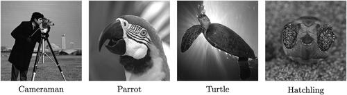In order to have a fair comparison, we use a Huber TV regularization for the corresponding lower lever problem, with the latter substituted by the TV primal-dual optimality conditions, $$\begin{array}{c}u-\text{div}p-f=0\\ \max (|\nabla u|,\gamma )p-\alpha \nabla u=0,\end{array}$$ where α is now the spatially dependent regularization parameter for TV. We use the same values for the Huber parameter γ both in bilevel TV and bilevel TGV. The associated test images are depicted in Figure 3 with resolution $n=m=256.$ The first one is the well-known “Cameraman” image which essentially consists of a combination of piecewise constant parts and texture. The next two images, “Parrot” and “Turtle” contain large piecewise affine type areas, thus they are more suitable for the TGV prior. The final image “hatchling” is characterized by highly oscillatory patterns of various kinds, depicting sand in various degrees of focus.

Figure 3. Test images, resolution $256\times 256.$

Parameter values: For the lower level primal-dual TGV problem we used μ = 0, ν = 1, $\delta ={10}^{-5},$ ${\gamma }_0={\gamma }_1={10}^{-3},$ and a mesh size h = 1. For the H¹–projection, we set ${ϵ}_{\alpha }={10}^{-6},$ and we also weighted the discrete Laplacian Δ with $6\times {10}^4.$ For the lower and upper bounds of α₀ and α₁ we set here ${\underset{¯}{\alpha }}_0={10}^{-2},{\overline{\alpha }}_0=10$ and ${\underset{¯}{\alpha }}_1={10}^{-4},{\overline{\alpha }}_1=10.$ We also set ${\lambda }_1={10}^{-11}$ and when we spatially varied α₀ we also set ${\lambda }_0={10}^{-11}.$ We used a normalized $n_w\times n_w$ filter for w (i.e., with entries $1/n_w^2$), with n_w = 7. The local variance barriers ${\underset{¯}{\sigma }}^2$ and ${\overline{\sigma }}^2$ were set according to (5.10). For our noisy images we have ${\sigma }^2={10}^{-2},$ and thus the corresponding values for $(\underset{¯}{\sigma },\overline{\sigma })$ are $(0.00798,0.01202).$ For the Armijo line search the parameters were ${\tau }_0^0=0.05,$ ${\tau }_1^0=100,c={10}^{-9},{\theta }_{-}=0.25,{\theta }_{+}=2.$ We solved each lower level problem until the residual of each of the optimality conditions (5.1)–(5.4) had Euclidean norm less than ${10}^{-4}.$ MATLAB’s backslash was used for the solution of the linear systems.

We note that the initialization of the algorithm needs some attention. As it was done in [29] for the TV case, ${\alpha }_0^0$ and ${\alpha }_0^1$ must be large enough in order to produce cartoon-like images, providing the local variance estimator with useful information. However, if α₀ is initially too large then there is a danger of falling into the regime, in which the TGV functional and hence the solution map of (at least the non-regularized) lower level problem does not depend on α₀. In that case the derivative of the reduced functional with respect to α₀ will be close to zero, thus making no or little progress with respect to its optimal choice. Indeed this was confirmed after some numerical experimentation. Note that an analogous phenomenon can occur also in the case where α₀ is much smaller than α₁. In that case it is the effect of α₁ which vanishes. This has been shown theoretically in [37, Proposition 2] for dimension one, but numerical experiments indicate that this phenomenon persists also in higher dimensions. 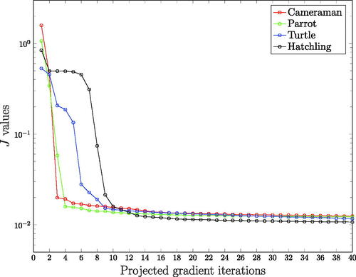In our examples we used ${\alpha }_1^0=0.25$ and ${\alpha }_0^0=0.2.$ Regarding the termination of the projected gradient algorithm, we used a fixed number of iterations n = 40. Neither the upper level objective nor the argument changed significantly after running the algorithm for more iterations; see for instance Figure 4. The same holds true for the corresponding PSNR and SSIM values. We also note that a termination criterion as in [29] based on the proximity measures $\Vert P_{{({\mathcal{A}}_{ad}^i)}_h}({\alpha }_i^k-{\nabla }_{{\alpha }_i}\widehat{J}({\alpha }_0^k,{\alpha }_1^k))-{\alpha }_i^k{\Vert }_{H^1({\Omega }_h)},$ i = 0, 1, is also possible here.

Figure 4. Upper level objective values vs projected gradient iterations for the problem (${\mathbb{P}}_{\text{TGV}}^h$) (right) of Figure 5 (scalar α₀, spatial α₁).

We note that due to the line search, the number of times that the lower level problem has to be solved is more than the number of projected gradient iterations. For instance for the four examples Figure 4 the lower level problem had to be solved 58, 57, 57, and 57 times, respectively, with typically 8-12 Newton iterations needed per each lower level problem, This resulted in each bilevel problem (40 projected gradient iterations) requiring approximately 45-50 times the CPU time needed to solve one instance of the lower level problem. We note however that in general after 8-9 projected gradient iterations the PSNR and SSIM values of the reconstruction were essentially reaching their top values, requiring about 6-8 times the CPU time needed for the lower level problem. Further improvement with respect to computational times can be achieved using faster descent methods than the one we used here, like for instance [55,56].

For the first series of examples we keep the parameter α₀ scalar, whose value nevertheless is determined by the bilevel algorithms. We depict the examples in Figure 5. The first row shows the noisy images, while the second contains the bilevel TV results. The third row depicts the best scalar TGV results with respect to SSIM, where we have computed the optimal scalars ${\alpha }_0,{\alpha }_1$ with a manual grid method. The fourth row shows the results of (${\mathbb{P}}_{\text{TGV}}^h$). Detailed sections of all the images of Figure 5 are highlighted in Figure 6. The weight functions α₁ for the bilevel TV and the bilevel TGV algorithms are shown in Figure 7. In Table 1 we report all PSNR and SSIM values of the best scalar methods (scalar TV, scalar TGV) with respect to both quality measures, the corresponding values of the bilevel TV and TGV algorithms, as well as the ones the correspond to solving the bilevel TGV with the statistics-based upper level objective (4.2) but using scalar parameters only (third row from the end in Table 1). For the latter case, we used no additional regularization for the weights in the upper level objective. We also report the PSNR and SSIM values of the computed results when both α₀, α₁ are spatially varying (last row), which we discuss later on in this section. We next comment on the results for each image.

Figure 5. First row: noisy images. Second row: bilevel TV. Third row: Best scalar TGV (SSIM). Fourth row: bilevel TGV.

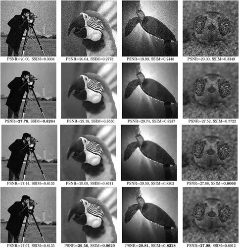
Figure 6. Details of the reconstructions shown in Figure 5.

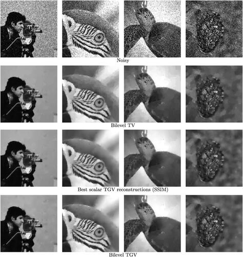
Figure 7. First row: the computed regularization functions α for bilevel TV. Second row: the computed regularization functions α₁ for bilevel TGV.

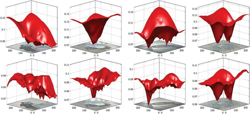
Table 1. PSNR and SSIM comparisons for the images of Figure 5.

${\sigma }^2=0.01$	Cameraman	Parrot	Turtle	Hatchling
Scalar TV (best PSNR)	27.69, 0.7962	29.25, 0.8354	29.49, 0.8032,	27.75, 0.7701
Scalar TV (best SSIM)	27.44, 0.8118	28.93, 0.8508	29.38, 0.8112	27.62, 0.7759
Bilevel $\text{TV}$ spatial α	$\mathbf{2}\mathbf{7}.\mathbf{7}\mathbf{8},\mathbf{0}.\mathbf{8}\mathbf{2}\mathbf{6}\mathbf{4}$	29.18, 0.8550	29.74, 0.8237	27.52, 0.7722
Scalar TGV (best PSNR)	27.68, 0.7813	29.47, 0.8504	29.63, 0.8223	$\mathbf{2}\mathbf{8}.\mathbf{0}\mathbf{5},$ 0.7950
Scalar TGV (best SSIM)	27.44, 0.8135	29.09, 0.8611	29.50, 0.8303	27.88, $\mathbf{0}.\mathbf{8}\mathbf{0}\mathbf{6}\mathbf{6}$
Bilevel TGV scalar α0, scalar α1	27.63, 0.8063	29.41, 0.8560	29.63, 0.8200	27.70, 0.7851
Bilevel TGV scalar α0, spatial α1	27.67, 0.8135	29.56, 0.8629	$\mathbf{2}\mathbf{9}.\mathbf{8}\mathbf{1},\mathbf{0}.\mathbf{8}\mathbf{3}\mathbf{2}\mathbf{8}$	27.98, 0.8012
Bilevel TGV spatial α0, spatial α1	27.68, 0.8151	$\mathbf{2}\mathbf{9}.\mathbf{5}\mathbf{8},\mathbf{0}.\mathbf{8}\mathbf{6}\mathbf{4}\mathbf{3}$	29.76, $\mathbf{0}.\mathbf{8}\mathbf{3}\mathbf{2}\mathbf{8}$	27.97, 0.8009

Every cell contains the corresponding PSNR and SSIM value.

Cameraman: Here both the best PSNR and SSIM are obtained by the bilevel TV algorithm. This is probably not surprising due to the piecewise constant nature of this image. However, the bilevel TGV algorithm improve upon its scalar version with respect to both measures.

Parrot: Here the best results with respect to both PSNR and SSIM are achieved by the bilevel TGV algorithm, (${\mathbb{P}}_{\text{TGV}}^h$). There is significant improvement over all TV methods, which is due to the parameters being chosen in a way such that the staircasing effect diminishes. Furthermore, we observe improvement over the scalar TGV result especially around the parrot’s eye, where the weights α₁ drop significantly; see the second column of Figure 7.

Turtle: We get analogous results here as well, with the bilevel TGV (${\mathbb{P}}_{\text{TGV}}^h$) producing the best results both with respect to PSNR and SSIM. There is a significant reduction of the staircasing effect, while the weight α₁ drops in the detailed areas of the image (head and flipper of the turtle).

Hatchling: In this image, the best PSNR and best SSIM are achieved by the scalar TGV when its parameters are manually optimized with respect to each measure (using the ground truth). However, the (ground truth-free) bilevel TGV achieves a better SSIM and PSNR value compared to these two results, respectively, achieving a better balance with respect to these measures. Similarly the scalar TV results are generally better than the ones of bilevel TV. We attribute this to the fact that the natural oscillatory features of the image are interpreted as noise by the upper level objective. Nevertheless, all the bilevel methods are able to locate and preserve better the eyes area, i.e., sand in focus, with the weight α₁ dropping there significantly.

We remark that in all four examples, the ground truth-free bilevel TGV with at least one spatially varying parameter always produces better results with respect to both PSNR and SSIM, than the corresponding ground truth-free bilevel TGV with both parameters being scalar, compare the third last with the second last row of Table 1.

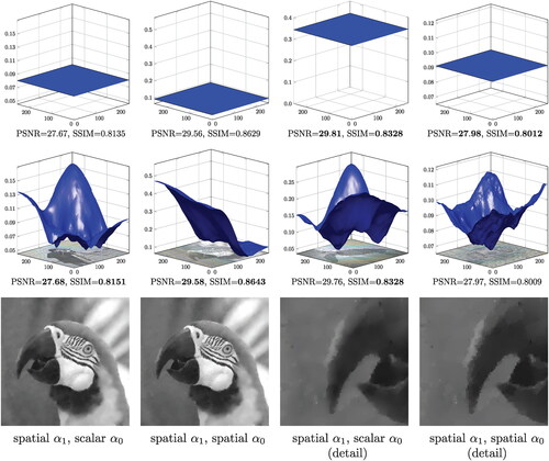
Finally, we would like to experiment with the case were also the weight α₀ varies spatially. We note that by spatially varying both TGV parameters, the reduced problem becomes highly non-convex with many combinations of these parameters leading to similar values for the upper level objective. In order to deal with this, we solve a slightly different problem by performing one step of alternating optimization. Here we optimize only with respect to a spatially varying α₀ having fixed the spatial weight α₁ as it has been computed by the previous experiments, see the last row of Figure 7. According to our numerical experiments, this strategy produces satisfactory results. As initialization for α₀, we set it constant, equal to 5.

In Figure 8 we depict the computed spatially varying parameters α₀ as well as the corresponding PSNR and SSIM values. Observe that the shape of α₀ is different to the one of α₁, compare the last row of Figure 7 to the second row of Figure 8. This implies that a non-constant ratio of ${\alpha }_0/{\alpha }_1$ is preferred throughout the image domain. Secondly, by spatially varying α₀ we only get a slight improvement with respect to PSNR and SSIM in the first two images, compare the second last and the last row of Table 1. However, it is interesting to observe the spatial adaptation of α₀ with respect to piecewise constant versus piecewise smooth areas. The values of α₀ are high in large piecewise constant areas, like the background of cameraman, the left area of the parrot image, as well as the top-right and the bottom-left corner of the turtle image. This is not so surprising as large values of α₀ imply a large ratio ${\alpha }_0/{\alpha }_1$ and a promotion of TV like behavior in those areas. We can observe this in more detail at the parrot image, see last row of Figure 8. On the contrary, the values of α₀ are kept small in piecewise smooth areas like the right part of the parrot image and the sun rays around the turtle’s body. This results in low ratio ${\alpha }_0/{\alpha }_1$ and thus to a more TGV like behavior, reducing the staircasing effect. This is another indication of the fact that by minimizing the statistics-based upper level objective one is able not only to better preserve detailed areas but also to finely adjust the TGV parameters such that the staircasing is reduced.

Figure 8. Experiments with optimizing over a spatially varying α₀. Top row: the automatically computed scalar parameters α₀, that correspond to the images of the last row of Figure 5. Middle row: the automatically computed spatially varying parameters α₀, where α₁ has been kept fixed (last row of Figure 7). The weight α₀ is adapted to piecewise constant parts having there large values and hence promoting TV like behavior, see for instance the parrot image at the last row. On the contrary α₀ has low values in piecewise smooth parts promoting a TGV like behavior reducing the staircasing.

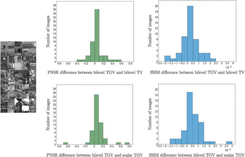
Lastly, we would like to see the degree of improvement of bilevel TGV with spatial parameters over the other ground truth-free approaches, i.e. using the statistics-based upper level objective, over a larger set of images. We thus used the 24 images of the Kodak dataset http://r0k.us/graphics/kodak/, and selected two middle square parts from each photograph, resized to 256 × 256 pixels, see left part of Figure 9. We added two more photographs (see bottom-right part in the depicted collection) to reach 50 photographs in total. In each photograph, we run the bilevel TV and bilevel TGV experiments after adding the same type of Gaussian noise (with only α₁ being spatially varying), as well as the bilevel TGV with both parameters to be scalar and we compared the corresponding PSNR differences, ${\text{PSNR}}_{\mathit{spatial}\mathrm{ }\text{TGV}}-{\text{PSNR}}_{\mathit{spatial}\mathrm{ }\text{TV}},$ ${\text{PSNR}}_{\mathit{spatial}\mathrm{ }\text{TGV}}-{\text{PSNR}}_{\mathit{scalar}\mathrm{ }\text{TGV}},$ as well as the corresponding SSIM ones, for every one of the 50 images. The PSNR improvement for the bilevel TGV over bilevel TV (both spatial parameters) was 0.05 ± 0.14 (mean ± standard deviation) while the improvement with respect to SSIM was more moderate, 0.003 ± 0.008. In Figure 9 (top) we also show the corresponding histograms of this difference. The fact that for some images the bilevel TV algorithm produces images of higher PSNR and/or SSIM, as it was the case for the cameraman, is perhaps not so surprising as the same has been observed in similar tests in [26] in the case of scalar parameters only and for a bilevel scheme that maximizes the PSNR of the reconstructed image, using a ground truth-based upper level objective. We stress that for large ratio ${\alpha }_0/{\alpha }_1$ TGV is equivalent to TV only up an affine correction [37] and for images that have a piecewise constant structure, setting α₀ in TGV to be large enough might not be enough to achieve the same reconstruction as TV. On the other hand the improvement of bilevel TGV with spatially varying α₁ versus its scalar analogue was $0.08\pm 0.17$ for the PSNR and 0.005 ± 0.008 for the SSIM, see bottom histograms of Figure 9. We note that the last two methods require a similar computational effort since the additional H¹–projection for the spatially varying weight is typically quite fast and does not significantly contribute to the overall computational time.

Figure 9. Histograms of the PSNR and SSIM differences between the bilevel spatial TGV and bilevel spatial TV (top) and between the bilevel spatial TGV and bilevel scalar TGV (bottom), for reconstructions of noisy versions of the 50 images on the left. In all bilevel algorithms the ground truth-free statistics-based upper level objective was used.

7. Conclusion

In this work we have adapted the bilevel optimization framework of [27, 29] for automatically computing spatially dependent regularization parameters for the TGV regularizer. We established a rigorous dualization framework for the lower level TGV minimization problem that formed the basis for its algorithmic treatment via a Newton method. We showed that the bilevel optimization framework with the statistics/localized residual based upper level objective is able to automatically produce spatially varying parameters that not only adapt to the level of detail in the image but also reduce the staircasing effect.

Future continuation of this work includes adaptation of the bilevel TGV framework for advanced inverse problems tasks, i.e., Magnetic Resonance Imaging (MRI) and Positron Emission Tomography (PET) reconstruction as well as in multimodal medical imaging problems where structural TV based regularizers (edge aligning) have been suggested. That will also require devising a bilevel scheme where the invertibility assumption on T is dropped, since the linear operators involved in these inverse problems do not satisfy this assumption. Adaptation of the framework for different noise distributions e.g. Poisson, Salt & Pepper as well as combination of those [57,58], should also be investigated. Finally, a fine structural analysis of the weighted TGV regularized solutions in the spirit of [59,60] would be also of interest.

Additional information

Funding

This work is funded by the Deutsche Forschungsgemeinschaft (DFG, German Research Foundation) under Germany’s Excellence Strategy – The Berlin Mathematics Research Center MATH+ (EXC-2046/1, project ID: 390685689). It was further supported by the MATHEON Research Center project CH12 funded by the Einstein Center for Mathematics (ECMath) Berlin. M.H and K.P. acknowledge support of Institut Henri Poincaré (UMS 839 CNRS-Sorbonne Université), and LabEx CARMIN (ANR-10-LABX-59-01). C.N.R. was supported by NSF grant DMS-2012391. H.S. acknowledges the financial support of Alexander von Humboldt Foundation.

Appendix A

We provide here the proof of Proposition 2.2:

Proof of Proposition 2.2

. The proof follows [12, Proposition 3.3]. Denote by $C_{\mathit{\alpha }},K_{\mathit{\alpha }}$ the following convex sets (A.1) $$C_{\mathit{\alpha }}=\left\{{\text{div}}^2\varphi :\varphi \in C_c^{\infty }(\Omega ,{\mathcal{S}}^{d\times d}),|\varphi (x)|\le {\alpha }_0(x),|\text{div}\varphi (x)|\le {\alpha }_1(x),\mathrm{ }\text{for}\mathrm{ }\text{all}\mathrm{ }x\in \Omega \right\},$$(A.1) (A.2) $$K_{\mathit{\alpha }}=\left\{{\text{div}}^{2}p:p\in H_0({\text{div}}^2;\Omega ),|p(x)|\le {\alpha }_0(x),|\text{div}p(x)|\le {\alpha }_1(x),\text{fora}.\mathrm{e}.\mathrm{x}\in \Omega \right\}.$$(A.2)

It suffices to show that (A.3) $${\overline{C_{\mathit{\alpha }}}}^{L^2(\Omega )}=K_{\mathit{\alpha }}.$$(A.3)

We first show that $K_{\mathit{\alpha }}$ is closed in $L^2(\Omega ).$ Let $g\in L^2(\Omega )$ and assume that there exists ${(p_n)}_{n\in \mathbb{N}}\subset H_0({\text{div}}^2;\Omega )$ where every p_n satisfies the convex constraints and ${\text{div}}^2{p}_n\to g$ in $L^2(\Omega ).$ By boundedness of ${\alpha }_0,{\alpha }_1$ we have that there exist $h_0\in L^2(\Omega ,{\mathcal{S}}^{d\times d}),$ $h_1\in L^2(\Omega ,{\mathbb{R}}^d)$ and a subsequence of ${(p_{n_k})}_{k\in \mathbb{N}}$ such that $$p_{n_k}\rightharpoonup h_0\hspace{1em}\text{and}\hspace{1em}\text{div}{p}_{n_k}\rightharpoonup h_1,$$ in $L^2(\Omega )$ and $L^2(\Omega ,{\mathbb{R}}^d),$ respectively. Using that, we have for every $\varphi \in C_c^{\infty }(\Omega ,{\mathbb{R}}^d)$ (A.4) $${\int }_{\Omega }\nabla \varphi ·h_0 dx=\underset{k\to \infty }{\lim }{\int }_{\Omega }\nabla \varphi ·p_{n_k} dx=-\underset{k\to \infty }{\lim }{\int }_{\Omega }\varphi ·\text{div}{p}_{n_k} dx=-{\int }_{\Omega }\varphi ·h_1 dx,$$(A.4) thus $h_1=\text{div}{h}_0.$ Similarly we derive that $g=\text{div}{h}_1={\text{div}}^2{h}_0$ and hence $h_0\in H({\text{div}}^2;\Omega ).$ Finally note that the set $$\left\{(h,\text{div}h,{\text{div}}^{2}h):h\in H_0({\text{div}}^2;\Omega ),|h(x)|\le {\alpha }_0(x),|\text{div}h(x)|\le {\alpha }_1(x),\text{fora}.\mathrm{e}.\mathrm{x}\in \Omega \right\},$$ is a norm-closed and convex subset of $L^2(\Omega ,({\mathcal{S}}^{d\times d}\times {\mathbb{R}}^d\times \mathbb{R}))$ and hence weakly closed. Since ${(p_{n_k},\text{div}{p}_{n_k},{\text{div}}^2{p}_{n_k})}_{k\in \mathbb{N}}$ belongs to that set, converging weakly to $(h_0,\text{div}{h}_0,{\text{div}}^2{h}_0)$ we get that the latter also belongs there. Thus, $K_{\mathit{\alpha }}$ is closed in $L^2(\Omega )$ and since $C_{\mathit{\alpha }}\subset K_{\mathit{\alpha }},$ we get ${\overline{C_{\mathit{\alpha }}}}^{L^2(\Omega )}\subset K_{\mathit{\alpha }}.$

It remains to show the other direction, i.e., $K_{\mathit{\alpha }}\subset {\overline{C_{\mathit{\alpha }}}}^{L^2(\Omega )}.$ Toward that, note first that the functional ${\text{TGV}}_{\mathit{\alpha }}^2(\Omega ):L^2(\Omega )\to \overline{\mathbb{R}},$ can also be written as $${\text{TGV}}_{\mathit{\alpha }}^2(u)={\mathcal{I}}_{C_{\mathit{\alpha }}}^{\ast }(u).$$

Using the convexity of $C_{\mathit{\alpha }}$ one gets $${\text{TGV}}_{\mathit{\alpha }}^{2^{ \ast }}(v)={\mathcal{I}}_{C_{\mathit{\alpha }}}^{\ast \ast }(v)={\mathcal{I}}_{{\overline{C_{\mathit{\alpha }}}}^{L^2(\Omega )}}(v).$$

Secondly, note that due to the lower bounds on ${\alpha }_0,{\alpha }_1,$ for $u\in L^2(\Omega ),$ we have that ${\text{TGV}}_{\mathit{\alpha }}^2(u)<\infty$ if and only if $u\in \text{BV}(\Omega ).$ Indeed this holds from the equivalence of the (scalar) $\Vert ·{\Vert }_{\text{BGV}}$ with $\Vert ·{\Vert }_{\text{BV}(\Omega )}$ and from the estimate $${\text{TGV}}_{\underset{¯}{\alpha },\underset{¯}{\alpha }}^2(u)\le {\text{TGV}}_{\mathit{\alpha }}^2(u)\le \Vert {\alpha }_1{\Vert }_{\infty }\text{TV}(u),$$ for every $u\in L^2(\Omega ).$ This means that if for ${\text{div}}^{2}p\in K_{\mathit{\alpha }}$ it holds (A.5) $${\int }_{\Omega }u {\text{div}}^{2}p dx\le {\text{TGV}}_{\mathit{\alpha }}^2(u),\hspace{1em}\text{for}\mathrm{ }\text{all}\mathrm{ }u\in \text{BV}(\Omega )\cap L^2(\Omega ),$$(A.5) then in fact the inequality (A.5) will hold for every $u\in L^2(\Omega )$ and thus ${\text{TGV}}_{\mathit{\alpha }}^{2^{ \ast }}({\text{div}}^{2}p)=0$ which implies ${\text{div}}^{2}p\in {\overline{C_{\mathit{\alpha }}}}^{L^2(\Omega )}.$ Thus in order to finish the proof it suffices to show (A.5) for every ${\text{div}}^{2}p\in K_{\mathit{\alpha }}.$ In view of Proposition 2.1 it suffices to show (A.6) $${\int }_{\Omega }u {\text{div}}^{2}p dx\le \underset{w\in \text{BD}(\Omega )}{\min }{\int }_{\Omega }{\alpha }_1 d|Du-w|+{\int }_{\Omega }{\alpha }_0 d\left|\mathcal{E}w\right|$$(A.6) for all $u\in \text{BV}(\Omega )\cap L^2(\Omega ).$ The first step toward that is to show that for every $w\in \text{BD}(\Omega )$ and for every $p\in H_0({\text{div}}^2;\Omega )$ with $|p(x)|\le {\alpha }_0(x)$ and $|\text{div}p(x)|\le {\alpha }_1(x)$ for a.e. $x\in \Omega ,$ it holds (A.7) $${\int }_{\Omega }w·\text{div}p dx\le {\int }_{\Omega }{\alpha }_0 d\left|\mathcal{E}w\right|.$$(A.7)

Indeed, note first that from (2.3), we get for every $\varphi \in C^{\infty }(\overline{\Omega },{\mathbb{R}}^d)$ (A.8) $$\left|{\int }_{\Omega }\varphi ·\text{div}p dx\right|=\left|{\int }_{\Omega }p·E\varphi dx\right|\le {\int }_{\Omega }|p\left|\right|E\varphi | dx\le {\int }_{\Omega } {\alpha }_0 d|E\varphi |.$$(A.8)

Recall now that every $w\in \text{BD}(\Omega )$ can be strictly approximated by a sequence ${({\varphi }_n)}_{n\in \mathbb{N}}\subset C^{\infty }(\overline{\Omega },{\mathbb{R}}^d),$ that is ${\varphi }_n\to w$ in $L^1(\Omega ,{\mathbb{R}}^d)$ and $\left|E\varphi \right|(\Omega )\to \left|\mathcal{E}w\right|(\Omega ),$ see [12, Proposition 2.10]. Furthermore, using that, along with Reshetnyak’s continuity theorem [33, Theorem 2.39] we also get that $${\int }_{\Omega }{\alpha }_0 d\left|E{\varphi }_n\right|\to {\int }_{\Omega }{\alpha }_0 d\left|\mathcal{E}w\right|,\hspace{1em}\text{as}\mathrm{ }n\to \infty .$$

Using the above and the fact that $\text{div}p\in L^{\infty }(\Omega ,{\mathbb{R}}^d),$ by taking limits in (A.8) we obtain (A.7). Finally in order to obtain (A.5) let again $p\in H_0({\text{div}}^2;\Omega )$ with $|p(x)|\le {\alpha }_0(x)$ and $|\text{div}p(x)|\le {\alpha }_1(x)$ for a.e. $x\in \Omega ,$ and let $\varphi \in C^{\infty }(\overline{\Omega },\mathbb{R}).$ Then by using (2.4) and (A.7), we have for every $w\in \text{BD}(\Omega )$ $$\begin{array}{c}{\int }_{\Omega }\varphi {\text{div}}^{2}p dx\le \left|{\int }_{\Omega }\nabla \varphi ·\text{div}p dx\right|=\left|{\int }_{\Omega }(\nabla \varphi -w)·\text{div}p dx+{\int }_{\Omega }w \text{div}p dx\right|\\ \le {\int }_{\Omega }|\nabla \varphi -w\left|\right|\text{div}p| dx+{\int }_{\Omega }{\alpha }_0 d|\mathcal{E}w|\le {\int }_{\Omega }{\alpha }_1|\nabla \varphi -w| dx+{\int }_{\Omega }{\alpha }_0 d|\mathcal{E}w|.\end{array}$$

Similarly as before given $u\in \text{BV}(\Omega )\cap L^2(\Omega )$ and $w\in \text{BD}(\Omega ),$ there exists a sequence ${({\varphi }_n)}_{n\in \mathbb{N}}\subset C^{\infty }(\overline{\Omega },\mathbb{R})$ such that ${\varphi }_n\to u$ in $L^2(\Omega )$ and $|\nabla {\varphi }_n-w|(\Omega )\to |Du-w|(\Omega ).$ This follows from a modification of the proof of [12, Proposition 2.10] where one takes advantage of the L² integrability of u. Using again the Reshetnyak’s continuity theorem and taking limits we get that for every $w\in \text{BD}(\Omega )$ $${\int }_{\Omega }u {\text{div}}^{2}p dx\le {\int }_{\Omega }{\alpha }_1 d|Du-w|+{\int }_{\Omega }{\alpha }_0 d\left|\mathcal{E}w\right|.$$

By taking the minimum over $w\in \text{BD}(\Omega ),$ we obtain (A.5). □

References

- Adams, R. A., Fournier, J. (2003). Sobolev Spaces. 2nd ed. Cambridge, MA: Academic Press,
- Ambrosio, L., Fusco, N., Pallara, D. (2000). Functions of Bounded Variation and Free Discontinuity Problems. USA: Oxford University Press.
- Attouch, H., Brezis, H. (1986). Duality for the Sum of Convex Functions in General Banach Spaces. Vol. 34, North-Holland Mathematical Library, pp. 125–133.
- Barzilai, J., Borwein, J. M. (1988). Two-point step size gradient methods. IMA J Numer Anal. 8(1):141–148. DOI: 10.1093/imanum/8.1.141.
- Benning, M., Brune, C., Burger, M., Müller, J. (2013). Higher-order TV methods: Enhancement via Bregman iteration. J Sci Comput. 54(2-3):269–310. DOI: 10.1007/s10915-012-9650-3.
- Bergounioux, M., Papoutsellis, E., Stute, S., Tauber, C. (2018). Infimal convolution spatiotemporal PET reconstruction using total variation based priors, HAL preprint https://hal.archives-ouvertes.fr/hal-01694064.
- Borwein, J. M., Vanderwerff, J. D. (2010). Convex Functions. Cambridge: Cambridge University Press.
- Bredies, K., Dong, Y., Hintermüller, M. (2013). Spatially dependent regularization parameter selection in total generalized variation models for image restoration. Inter. J. Comput. Math. 90(1):109–123. DOI: 10.1080/00207160.2012.700400.
- Bredies, K., Holler, M. (2012). Artifact-free JPEG decompression with total generalized variation. VISAP 2012: Proceedings of the International Conference on Computer Vision and Applications,
- Bredies, K., Holler, M. (2013). A TGV regularized wavelet based zooming model. Scale Space and Variational Methods in Computer Vision. Springer, DOI: 10.1007/978-3-642-38267-3_13., pp. 149–160.
- Bredies, K., Holler, M. (2014). Regularization of linear inverse problems with total generalized variation. J. Inverse Ill-Posed Prob. 22(6):871–913. DOI: 10.1515/jip-2013-0068.
- Bredies, K., Holler, M. (2015). A TGV-based framework for variational image decompression, zooming, and reconstruction. Part I: Analytics. SIAM J. Imaging Sci. 8(4):2814–2850. DOI: 10.1137/15M1023865.
- Bredies, K., Holler, M. (2015). A TGV-based framework for variational image decompression, zooming, and reconstruction. Part II: Numerics. SIAM J. Imaging Sci. 8(4):2851–2886. DOI: 10.1137/15M1023877.
- Bredies, K., Holler, M., Storath, M., Weinmann, A. (2018). Total generalized variation for manifold-valued data. SIAM J. Imaging Sci. 11(3):1785–1848. DOI: 10.1137/17M1147597.
- Bredies, K., Kunisch, K., Pock, T. (2010). Total generalized variation. SIAM J. Imaging Sci. 3(3):492–526. DOI: 10.1137/090769521.
- Bredies, K., Kunisch, K., Valkonen, T. (2013). Properties of L1-TGV 2: The one-dimensional case. J. Math. Anal. Appl. 398(1):438–454. DOI: 10.1016/j.jmaa.2012.08.053.
- Bredies, K., Valkonen, T. (2011). Inverse problems with second-order total generalized variation constraints. Proceedings of SampTA 2011 - 9th International Conference on Sampling Theory and Applications, Singapore,
- Burger, M., Papafitsoros, K., Papoutsellis, E., Schönlieb, C. B. (2016). Infimal convolution regularisation functionals of BV and [Formula: see text] Spaces: Part I: The Finite [Formula: see text] Case. J. Math. Imaging Vis. 55(3):343–369. DOI: 10.1007/s10851-015-0624-6.
- Calatroni, L., Chung, C., Los Reyes, J. D., Schönlieb, C. B., Valkonen, T. (2017). Bilevel approaches for learning of variational imaging models. RADON Book Series on Computational and Applied Mathematics. Vol. 18, Berlin, Boston: De Gruyter, https://www.degruyter.com/view/product/458544.
- Calatroni, L., De Los Reyes, J. C., Schönlieb, C. B. (2017). Infimal convolution of data discrepancies for mixed noise removal. SIAM J. Imaging Sci. 10(3):1196–1233. DOI: 10.1137/16M1101684.
- Calatroni, L., Papafitsoros, K. (2019). Analysis and automatic parameter selection of a variational model for mixed gaussian and salt-and-pepper noise removal. Inverse Prob. 35(11):114001. DOI: 10.1088/1361-6420/ab291a.
- Caselles, V., Chambolle, A., Novaga, M. (2007). The discontinuity set of solutions of the TV denoising problem and some extensions. Multiscale Model. Simul. 6(3):879–894. DOI: 10.1137/070683003.
- Chambolle, A., Duval, V., Peyré, G., Poon, C. (2017). Geometric properties of solutions to the total variation denoising problem. Inverse Prob. 33(1):015002. http://stacks.iop.org/0266-5611/33/i=1/a=015002. DOI: 10.1088/0266-5611/33/1/015002.
- Chambolle, A., Lions, P. L. (1997). Image recovery via total variation minimization and related problems. Numerische Mathematik. 76(2):167–188. DOI: 10.1007/s002110050258.
- Van Chung, C., De los Reyes, J. C., Schönlieb, C. B. (2017). Learning optimal spatially-dependent regularization parameters in total variation image denoising. Inverse Prob. 33(7):074005. DOI: 10.1088/1361-6420/33/7/074005.
- De Los Reyes, J. C., Schönlieb, C. B., Valkonen, T. (2016). The structure of optimal parameters for image restoration problems. J. Math. Anal. Appl. 434(1):464–500. DOI: 10.1016/j.jmaa.2015.09.023.
- De Los Reyes, J. C., Schönlieb, C. B., Valkonen, T. (2017). Bilevel parameter learning for higher-order Total Variation regularisation models. J. Math. Imaging Vis. 57(1):1–25. DOI: 10.1007/s10851-016-0662-8.
- Demengel, F., Temam, R. (1984). Convex functions of a measure and applications. Indiana Univ. Math. J. 33(5):673–709. DOI: 10.1512/iumj.1984.33.33036.
- Ekeland, I., Temam, R. (1999). Convex analysis and variational problems. Classics Appl. Mathem. Soci. Indust. Appl. Math.
- Girault, V., Raviart, P. A. (1986). Finite Element Method for Navier-Stokes Equation. Berlin, Germany: Springer.
- Hintermüller, M., Holler, M., Papafitsoros, K. (2018). A function space framework for structural total variation regularization with applications in inverse problems. Inverse Prob. 34(6):064002. http://stacks.iop.org/0266-5611/34/i=6/a=064002. DOI: 10.1088/1361-6420/aab586.
- Hintermüller, M., Kunisch, K. (2006). Path-following methods for a class of constrained minimization problems in function space. SIAM J. Optim. 17(1):159–187. DOI: 10.1137/040611598.
- Hintermüller, M., Papafitsoros, K. (2019). Generating structured nonsmooth priors and associated primal-dual methods. Processing, Analyzing and Learning of Images, Shapes, and Forms: Part 2. In: Ron K. and Xue-Cheng T., eds. Handbook of Numerical Analysis, Vol. 20, DOI: 10.1016/bs.hna.2019.08.001., pp. 437–502.
- Hintermüller, M., Papafitsoros, K., Rautenberg, C. N. (2017). Analytical aspects of spatially adapted total variation regularisation. J. Math. Anal. Appl. 454(2):891–935. DOI: 10.1016/j.jmaa.2017.05.025.
- Hintermüller, M., Papafitsoros, K., Rautenberg, C. N. (2020). Variable step mollifiers and applications. Integr. Equ. Oper. Theory. 92(6). DOI: 10.1007/s00020-020-02608-2.
- Hintermüller, M., Rautenberg, C. N. (2015). On the density of classes of closed convex sets with pointwise constraints in Sobolev spaces. J. Math. Anal. Appl. 426(1):585–593. DOI: 10.1016/j.jmaa.2015.01.060.
- Hintermüller, M., Rautenberg, C. N. (2017). Optimal selection of the regularization function in a weighted total variation model. Part I: Modelling and theory. J. Math. Imaging Vis. 59(3):498–514. DOI: 10.1007/s10851-017-0744-2.
- Hintermüller, M., Rautenberg, C. N., Rösel, S. (2017). Density of convex intersections and applications. Proc. Royal Soci. London A Math. Phys. Engng Sci. 473(2205) DOI: 10.1098/rspa.2016.0919.
- Hintermüller, M., Rautenberg, C. N., Wu, T., Langer, A. (2017). Optimal selection of the regularization function in a weighted total variation model. Part II: Algorithm, its analysis and numerical tests. J. Math. Imaging Vis. 59(3):515–533. DOI: 10.1007/s10851-017-0736-2.
- Hintermüller, M., Stadler, G. (2006). An infeasible primal-dual algorithm for total bounded variation–based inf-convolution-type image restoration. SIAM J. Sci. Comput. 28(1):1–23. DOI: 10.1137/040613263.
- Holler, M., Kunisch, K. (2014). On infimal convolution of TV-type functionals and applications to video and image reconstruction. SIAM J. Imaging Sci. 7(4):2258–2300. DOI: 10.1137/130948793.
- Huber, R., Haberfehlner, G., Holler, M., Kothleitner, G., Bredies, K. (2019). Total generalized variation regularization for multi-modal electron tomography. Nanoscale. 11(12):5617–5632. DOI: 10.1039/c8nr09058k.
- Jalalzai, K. Discontinuities of the minimizers of the weighted or anisotropic total variation for image reconstruction, arXiv preprint 1402.0026 (2014), http://arxiv.org/abs/1402.0026.
- Jalalzai, K. (2016). Some remarks on the staircasing phenomenon in total variation-based image denoising. J. Math. Imaging Vis. 54(2):256–268. DOI: http://dx.doi.org/10.1007/s10851-015-0600-1.
- Knoll, F., Bredies, K., Pock, T., Stollberger, R. (2011). Second order total generalized variation (TGV) for MRI. Magn. Reson. Med. 65(2):480–491. DOI: 10.1002/mrm.22595.
- Knoll, F., Holler, M., Koesters, T., Otazo, R., Bredies, K., Sodickson, D. K. (2017). Joint MR-PET reconstruction using a multi-channel image regularizer. IEEE Trans. Med. Imaging. 36(1):1–16. DOI: 10.1109/TMI.2016.2564989.
- Kunisch, K., Hintermüller, M. (2004). Total bounded variation regularization as a bilaterally constrained optimization problem. SIAM J. Appl. Math. 64(4):1311–1333. DOI: 10.1137/S0036139903422784.
- Nesterov, Y. E. (1983). A method for solving the convex programming problem with convergence rate O(1/k2). Soviet Math. Dokl. 27:367–372.
- Papafitsoros, K. (2014). Novel higher order regularisation methods for image reconstruction. Ph.D. thesis. University of Cambridge. https://www.repository.cam.ac.uk/handle/1810/246692.
- Papafitsoros, K., Bredies, K. (2015). Department of Applied Mathematics and Theoretical Physics, University of Cambridge, Wilberforce Road, CB3 0WA, Cambridge A study of the one dimensional total generalised variation regularisation problem. Inverse Prob. Imaging. 9(2):511–550. DOI: 10.3934/ipi.2015.9.511.
- Papafitsoros, K., Valkonen, T. (2015). Asymptotic behaviour of total generalised variation. Scale Space and Variational Methods in Computer Vision: 5th International Conference, SSVM 2015, Proceedings. In: Jean-François A., Mila N., and Nicolas P., eds. Springer International Publishing, pp. 702–714. DOI: 10.1007/978-3-319-18461-6_56.
- Pöschl, C., Scherzer, O. (2015). Exact solutions of one-dimensional total generalized variation. Comm. Math. Sci. 13(1):171–202. DOI: 10.4310/CMS.2015.v13.n1.a9.
- Ring, W. (2000). Structural properties of solutions to total variation regularization problems. Esaim: M2an. 34(4):799–810. DOI: 10.1051/m2an:2000104.
- Rudin, L. I., Osher, S., Fatemi, E. (1992). Nonlinear total variation based noise removal algorithms. Physica D: Nonlinear Phenomena. 60(1-4):259–268. DOI: 10.1016/0167-2789(92)90242-F.
- Schloegl, M., Holler, M., Schwarzl, A., Bredies, K., Stollberger, R. (2017). Infimal convolution of total generalized variation functionals for dynamic MRI. Magn Reson Med. 78(1):142–155. DOI: 10.1002/mrm.26352.
- Temam, R. (1985). Mathematical Problems in Plasticity. Vol. 15, Gauthier-Villars Paris.
- Temam, R., Strang, G. (1980). Functions of bounded deformation. Arch. Rational Mech. Anal. 75(1):7–21. DOI: 10.1007/BF00284617.
- Valkonen, T. (2017). The jump set under geometric regularisation. Part 2: Higher-order approaches. J. Math. Anal. Appl. 453(2):1044–1085. DOI: 10.1016/j.jmaa.2017.04.037.
- Valkonen, T., Bredies, K., Knoll, F. (2013). Total generalized variation in diffusion tensor imaging. SIAM J. Imaging Sci. 6(1):487–525. DOI: 10.1137/120867172.
- Zowe, J., Kurcyusz, S. (1979). Regularity and stability for the mathematical programming problem in Banach spaces. Appl Math Optim. 5(1):49–62. DOI: 10.1007/BF01442543.