Autonomous distributed braking and driving force control architecture based on broadcast control for vehicles with in-wheel motors on four wheels

Abstract

In this paper, we investigate an architecture for autonomous distributed control of braking and driving force on each wheel of a vehicle equipped with in-wheel motors on four wheels. Specifically, in a scenario where the driving force of some wheels is reduced due to low-friction road or motor failure during going straight ahead, the remaining wheels that can generate driving force autonomously control the yaw rate caused by the unbalanced driving force and driving force reduction to maintain the vehicle behavior. To realize autonomous distributed control, we focus on broadcast control from the control theory of multi-agent systems, which deals with the control of systems composed of many elements. We verify by simulation that the proposed architecture performs as desired for the assumed scenario.

GRAPHICAL ABSTRACT

KEYWORDS:

• Autonomous distributed control
• broadcast control
• vehicle motion control
• in-wheel motor

1. Introduction

The introduction of electric vehicles (EVs) is accelerating in order to achieve carbon neutrality. In Europe, battery EVs account for 23% of all vehicles in 2022 and are expected to exceed 90% in 2035 [1], and the day when the ratio of internal combustion engine vehicles to EVs will reverse is becoming a reality.

Currently, the transition from internal combustion engines, which have a long history, to electric drives is underway, so various forms of electric energy supply coexist, including batteries, fuel cells, and range extenders, but the transition to motor drives is steadily progressing. Compared to engines, motors have a simpler hardware structure and dynamic characteristics, so differences in control by software can easily be seen as differences in vehicle performance, and it is important to note that there are high expectations for control technology.

An in-wheel motor system is being considered as one of the drivetrains for EVs. In-wheel motors placed at each wheel not only provide a high degree of freedom in the cabin layout, but also have the potential to dramatically improve vehicle dynamics by enabling independent control of the braking and driving force at each wheel. Furthermore, a unit combining an in-wheel motor and a steering motor that enables independent control of the steering angle of each wheel has recently been developed [2], and the degree of control freedom continues to increase. From the perspective of vehicle motion control, it is important to fully utilize the redundancy and degree of control freedom provided by the motor drive to achieve the desired vehicle behavior.

However, when handling controlled objects with high redundancy and control freedom within the framework of centralized control and rule-based algorithms, which have been the mainstream in internal combustion engine vehicles, there are issues such as increased communication volume and rule complexity. For this reason, the majority of EVs on the market use electric axles, i.e. a single motor connected to the left and right wheels via differential gears and driveshafts, which are easy to handle within the conventional framework, and the adoption of in-wheel motor systems has been sluggish [3,4].

In order to overcome the above issues, this study breaks through the conventional framework and discusses a method for braking and driving force distribution based on autonomous distributed control. In realizing autonomous distributed control, we focus on the control theory of multi-agent systems, which deals with the control of systems consisting of many elements. We propose a control architecture based on broadcast control [5,6], which can suppress communication volume and algorithm complexity even if redundancy and degree of control freedom are increased.

This paper is based on our preliminary version [7], published in the conference proceedings. This journal version contains the full explanations about our results, which are omitted in the conference version, and add new data to evaluate our method.

2. Problem setting

As a control system for EVs equipped with in-wheel motors, a system consisting of a braking and driving force controller and an observer for each wheel has been proposed, as shown in Figure 1 [8]. The controlled object for each controller and observer is the in-wheel motor (i.e. ‘IWM’ in Figure 1: including a PWM inverter and a control circuit implemented with vector control, etc.), with the motor torque target value $T_{\mathrm{ij}}^{\ast }$¹ as input and the angular velocity of the wheel ${\omega }_{\mathrm{ij}}$ as output. The dynamic characteristics between $T_{\mathrm{ij}}^{\ast }$ and ${\omega }_{\mathrm{ij}}$ are very simple. The relationship between $T_{\mathrm{ij}}^{\ast }$ and actual torque $T_{\mathrm{ij}}$ can be regarded as a first-order delay system, and the relationship between $T_{\mathrm{ij}}$ and ${\omega }_{\mathrm{ij}}$ as an inertial system.

Figure 1. Braking and driving force control system.

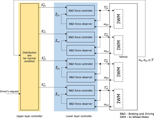
The braking and driving force controller has a wheel speed controller (not shown in Figure 1) in the inner loop, which calculates $T_{\mathrm{ij}}^{\ast }$ from the wheel speed target value derived from the slip ratio that matches the braking and driving force target value $X_{\mathrm{ij}}^{\ast }$ and the actual value $X_{\mathrm{ij}}$. Actual values of the braking and driving force $X_{\mathrm{ij}}$ are required for control, but the difficulty of directly measuring the force between the road surface and the tires necessitates an observer. The braking and driving force observer has a structure based on a disturbance observer and calculates the estimated braking and driving force ${\hat{X}}_{\mathrm{ij}}$ from the relationship between $T_{\mathrm{ij}}^{\ast }$ and ${\omega }_{\mathrm{ij}}$.

The distribution law located in the upper layer determines the braking and driving force target value $X_{\mathrm{ij}}^{\ast }$ for each wheel from the total front/rear braking and driving force target value $X_{+}^{\ast }$ and the total left/right braking and driving force difference target value $X_{-}^{\ast }$ so that the following relationship is satisfied. (1) $\begin{array}{r}\begin{array}{rl}{X}_{\mathrm{fr}}^{\ast }+X_{\mathrm{rr}}^{\ast }+X_{\mathrm{fl}}^{\ast }+X_{\mathrm{rl}}^{\ast }& =X_{+}^{\ast }\\ X_{\mathrm{fr}}^{\ast }+X_{\mathrm{rr}}^{\ast }-X_{\mathrm{fl}}^{\ast }-X_{\mathrm{rl}}^{\ast }& =X_{-}^{\ast }\end{array}\end{array}$(1) Note that $X_{+}^{\ast }$ and $X_{-}^{\ast }$ are determined by the driver's requests and vehicle conditions such as longitudinal and lateral acceleration $a_x,a_y$, yaw rate γ, and vehicle speed V. Since the combination of braking and driving force of each wheel that satisfies (1(1) $\begin{array}{r}\begin{array}{rl}{X}_{\mathrm{fr}}^{\ast }+X_{\mathrm{rr}}^{\ast }+X_{\mathrm{fl}}^{\ast }+X_{\mathrm{rl}}^{\ast }& =X_{+}^{\ast }\\ X_{\mathrm{fr}}^{\ast }+X_{\mathrm{rr}}^{\ast }-X_{\mathrm{fl}}^{\ast }-X_{\mathrm{rl}}^{\ast }& =X_{-}^{\ast }\end{array}\end{array}$(1) ) is not unique, it is formulated as an optimization problem to minimize or maximize some index [9]. Methods to minimize indices such as tire load factor [10,11] and energy consumption during driving [12,13] have been proposed. These methods assume that each wheel operates normally, i.e. follows the target value. Therefore, the following abnormal conditions, in which the wheels do not follow the target values, prevent proper distribution. For example, when a motor fails, or when driving force saturation occurs due to low-friction road or load transfer, and the braking and driving force controller activates the traction function to reduce the driving force to prevent tire spinning.

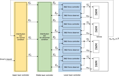
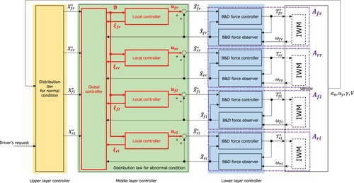
In this study, we focus on the problem of designing the braking and driving force distribution law for abnormal conditions. The distribution under normal and abnormal conditions is an essentially different problem. In the normal case, the problem is to determine the target values for all wheels, whereas in the abnormal case, the problem is to determine the target values for all wheels except the wheel with the abnormality. In other words, the problem is invariant under normal conditions, but under abnormal conditions, the number of decision variables changes according to the state of the abnormality. Therefore, it is generally necessary to divide cases based on abnormal conditions. Furthermore, the difference in terms of control requirements is that the distribution under abnormal conditions needs to be performed before wheel abnormalities affect vehicle behavior. For this reason, the braking and driving force of each wheel (i.e. actuator behavior) is directly monitored, and the target value under normal conditions is corrected and redistributed according to the abnormal conditions. As shown in Figure 2, it is positioned in the middle layer and requires an algorithm that can handle a shorter control period than the distribution under normal conditions. In Figure 2, ${\tilde{X}}_{\mathrm{ij}}^{\ast }$ represents the corrected target value for redistribution at each wheel. In order to maintain the vehicle behavior before and after an abnormality, ${\tilde{X}}_{\mathrm{ij}}^{\ast }$ must be determined so that the following relationship holds for both normal and abnormal wheels. (2) $\begin{array}{rl}{\hat{X}}_{\mathrm{fr}}+{\hat{X}}_{\mathrm{rr}}+{\hat{X}}_{\mathrm{fl}}+{\hat{X}}_{\mathrm{rl}}& =X_{+}^{\ast }\\ {\hat{X}}_{\mathrm{fr}}+{\hat{X}}_{\mathrm{rr}}-{\hat{X}}_{\mathrm{fl}}-{\hat{X}}_{\mathrm{rl}}& =X_{-}^{\ast }\end{array}$(2) Conventional methods for distribution in the event of an abnormality generally use centralized control that aggregates the status from each wheel and redistributes the braking and driving force to each wheel based on predefined compensation rules. Therefore, exhaustive compensation rules must be established at the design stage. Examples of compensation rules include: using the rear wheels to compensate for reduced driving force at the front wheels, the front wheels to compensate for reduced driving force at the rear wheels [14], and the steering system to compensate for moments caused by an imbalance between the left and right driving forces [15,16]. In addition, since the centralized controller needs to give instructions to each wheel, the communication volume from the centralized controller to the wheel controllers increases as the number of wheels increases. These previous studies remain problematic in terms of scalable handling of various scenarios and vehicle structures, such as the reduction of driving force at only one wheel, extension to multi-wheel vehicles and skid-steering vehicles without a steering system, and so on. The reason is that the increase in communication volume and the complexity of compensation rules are inevitable.

Figure 2. Layout of the distribution law for abnormal conditions.

In order to suppress the increase in communication volume and the complexity of compensation rules, we considered that it would be effective to shift the architecture from the conventional centralized control to an autonomous distributed control. For the architecture shifting, we focus on broadcast control, one of the multi-agent system control theories. The reason is that broadcast control provides a control framework in which an autonomous behavior of each agent achieves a single objective as a group of agents, and the distribution problem can be formulated by assigning the agent to each wheel and the objective of the agent group to the desired vehicle behavior. Furthermore, it should be noted that broadcast control consists of two types of controllers: a global controller and a local controller. The global controller, which is responsible for supervising a group of agents, only needs to evaluate the degree to which the agents have achieved their goals and does not need to give instructions to each agent. The local controller determines the behavior of each agent based on the results of the global controller's evaluation. The same local controller can be used for each agent. Also, thanks to broadcast communication, the communication volume from the global controller to the local controller does not depend on the number of agents. Broadcast control is highly scalable while avoiding a significant increase in communication volume, because control is achieved simply by preparing a local controller for each agent and increasing or decreasing parameters related to the number of agents in the global controller.

The above discussion is summarized. In this study, we consider a distribution law for abnormal conditions based on broadcast control. Specifically, we aim to design ${\tilde{X}}_{\mathrm{ij}}^{\ast }$ to maintains (2(2) $\begin{array}{rl}{\hat{X}}_{\mathrm{fr}}+{\hat{X}}_{\mathrm{rr}}+{\hat{X}}_{\mathrm{fl}}+{\hat{X}}_{\mathrm{rl}}& =X_{+}^{\ast }\\ {\hat{X}}_{\mathrm{fr}}+{\hat{X}}_{\mathrm{rr}}-{\hat{X}}_{\mathrm{fl}}-{\hat{X}}_{\mathrm{rl}}& =X_{-}^{\ast }\end{array}$(2) ) through the autonomous distributed behavior of each wheel without predefined compensation rules.

3. Main results

3.1. Broadcast control

An overview of broadcast control [6] is described below.

As shown in Figure 3, the broadcast control system consists of two types of controllers: a global controller G and a local controller $L_k$ corresponding to each agent $A_k(k\in \{1,2,\dots ,N\left\}\right)$. In the global controller, the achievement of the overall system goal is evaluated by an evaluation function, and in the local controller, the control input that minimizes the evaluation function is calculated. Broadcast control therefore provides a mechanism for minimizing the evaluation function, which is a coordination of the two controllers.

Figure 3. Broadcast control system.

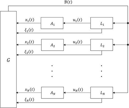
The global controller receives the state $x_k\left(t\right)\in {\mathbb{R}}^n$ from the agent $A_k$ and the random variable ${\xi }_k\left(t\right)\in {\mathbb{R}}^n$ from the local controller $L_k$. Note that $t\in \{0,1,2,\dots \}$ is the sampling time and each element of ${\xi }_k\left(t\right)$ is assumed to follow a Bernoulli distribution taking $\pm 1$ with probability 0.5.

In order to virtually change the state of each agent, we introduce a virtual input ${\overline{u}}_k\left(t\right)\in {\mathbb{R}}^n$ defined by the following equation. (3) $\begin{array}{r}{\overline{u}}_k\left(t\right)=b\left(t\right){\xi }_k\left(t\right)\end{array}$(3) $b\left(t\right)\in \mathbb{R}$ is the gain, given by using the constants $b_0,b_p,t_v$ common to each agent. (4) $\begin{array}{r}b\left(t\right)=\frac{b_0}{(t+t_v{)}^{b_p}}\end{array}$(4) The virtual state ${\overline{x}}_k(t+1)\in {\mathbb{R}}^n$ is determined from the virtual input ${\overline{u}}_k\left(t\right)$ according to the following dynamics. (5) $\begin{array}{r}{\overline{x}}_k(t+1)=x_k\left(t\right)+{\overline{u}}_k\left(t\right)\end{array}$(5) The evaluation function representing the degree of achievement of the overall system goal is defined as $J\left(x\right)\in {\mathbb{R}}^{\mathrm{nN}}\to \mathbb{R},x=[x_1^T\cdots x_N^T{]}^T\in {\mathbb{R}}^{\mathrm{nN}}$, and calculate the broadcast signal $\mathcal{B}\left(t\right)\in \mathbb{R}$ from the following equation. The collection of the virtual states is denoted by $\overline{x}=[{\overline{x}}_1^T\cdots {\overline{x}}_N^T{]}^T\in {\mathbb{R}}^{\mathrm{nN}}$. (6) $\begin{array}{r}\mathcal{B}\left(t\right)=J\left(\overline{x}\right(t+1\left)\right)-J\left(x\right(t\left)\right)\end{array}$(6) Each local controller receives $\mathcal{B}\left(t\right)$ from the global controller and determines the control input $u_k\left(t\right)\in {\mathbb{R}}^n$ to the agent as follows. That is, the local controller contains ${\xi }_k\left(t\right)$ and is given as a randomized controller. (7) $\begin{array}{r}{u}_k\left(t\right)=-a\left(t\right)\frac{\mathcal{B}\left(t\right)}{b\left(t\right)}{\xi }_k^{(-1)}\left(t\right)\end{array}$(7) $a\left(t\right)\in \mathbb{R}$ is the gain, given by using the constants $a_0,a_p,t_v$ common to each agent. (8) $\begin{array}{r}a\left(t\right)=\frac{a_0}{(t+t_v{)}^{a_p}}\end{array}$(8) Note that ${\xi }_k^{(-1)}\left(t\right)$ in (7(7) $\begin{array}{r}{u}_k\left(t\right)=-a\left(t\right)\frac{\mathcal{B}\left(t\right)}{b\left(t\right)}{\xi }_k^{(-1)}\left(t\right)\end{array}$(7) ) represents a vector consisting of the inverse of each element of the vector ${\xi }_k\left(t\right)$.

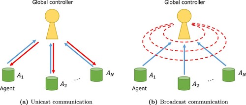
As can be seen from the above overview, the global controller is only responsible for evaluating the degree of achievement of the overall system goal and does not have the role of instructing each agent. Therefore, it only needs to send a common signal $\mathcal{B}\left(t\right)$ to each agent. On the other hand, each local controller calculates the inputs to the agent based only on $\mathcal{B}\left(t\right)$, so there is no need for communication between the local controllers. Thus, the communication volume can be reduced to $O(N+1)$ compared to $O\left(2N\right)$ of unicast communication in centralized control as shown in Figure 4, where N is the number of agents.

Figure 4. Communication between agents and a global controller. (a) Unicast communication and (b) Broadcast communication.

3.2. Autonomous distributed braking and driving force control architecture

By integrating broadcast control into the control system shown in Figure 2, we attempt to construct a control system shown in Figure 5 in which the remaining wheels operate in an autonomous distributed manner to maintain vehicle behavior in the event of an abnormality.

Figure 5. Braking and driving force control system with broadcast control.

In the control system shown in Figure 5, the system with ${\tilde{X}}_{\mathrm{ij}}^{\ast }$ as input and ${\hat{X}}_{\mathrm{ij}}$ as output is regarded as one agent. That is, the controller, observer, and in-wheel motor are collectively regarded as one agent. Four agents $A_{\mathrm{ij}}$ corresponding to four wheels are considered as controlled objects in this study. By incorporating the global controller and the local controller as shown by the red line in Figure 5, we construct a control system in which the target values $X_{\mathrm{ij}}^{\ast }$ are corrected and redistributed by broadcast control. The basic operation of the global and local controllers in Figure 5 follows that described in Section 3.1, but the unique point of this study is that separate evaluation functions are introduced for normal and abnormal conditions, and they are switched according to the presence or absence of abnormalities. This is described in detail below.

In the global controller, the virtual input ${\overline{u}}_{\mathrm{ij}}\left(t\right)\in \mathbb{R}$ is calculated from the random variable ${\xi }_{\mathrm{ij}}\left(t\right)\in \mathbb{R}$ received from each local controller and $b\left(t\right)$ given by (4(4) $\begin{array}{r}b\left(t\right)=\frac{b_0}{(t+t_v{)}^{b_p}}\end{array}$(4) ). The virtual input corresponds to minute fluctuations in the braking and driving force. (9) $\begin{array}{r}{\overline{u}}_{\mathrm{ij}}\left(t\right)=b\left(t\right){\xi }_{\mathrm{ij}}\left(t\right)\end{array}$(9) The virtual state ${\overline{X}}_{\mathrm{ij}}(t+1)\in \mathbb{R}$ (i.e. the virtual braking and driving force) is then calculated using the following equation based on (9(9) $\begin{array}{r}{\overline{u}}_{\mathrm{ij}}\left(t\right)=b\left(t\right){\xi }_{\mathrm{ij}}\left(t\right)\end{array}$(9) ) and ${\hat{X}}_{\mathrm{ij}}\left(t\right)\in \mathbb{R}$ received from each agent. (10) $\begin{array}{r}{\overline{X}}_{\mathrm{ij}}(t+1)={\hat{X}}_{\mathrm{ij}}\left(t\right)+{\overline{u}}_{\mathrm{ij}}\left(t\right)\end{array}$(10) The following two evaluation functions $J_a\left(X\right),J_n\left(X\right)\in \mathbb{R},X=[X_{\mathrm{fr}}{X}_{\mathrm{rr}}{X}_{\mathrm{fl}}{X}_{\mathrm{rl}}{]}^T\in {\mathbb{R}}^4$ are introduced and switched according to the presence or absence of abnormalities in the braking and driving force. The abnormalities in this study mean the cases where the actual braking and driving force of some wheel is insufficient to achieve the target value. (11) $\begin{array}{rl}{J}_a\left(X\right)& =W_{\mathrm{aX}}{\{X_{+}^{\ast }-(X_{\mathrm{fr}}+X_{\mathrm{rr}}+X_{\mathrm{fl}}+X_{\mathrm{rl}}\left)\right\}}^2\\ & +W_{\mathrm{a\gamma }}{\{X_{-}^{\ast }-(X_{\mathrm{fr}}+X_{\mathrm{rr}}-X_{\mathrm{fl}}-X_{\mathrm{rl}}\left)\right\}}^2\end{array}$(11) (12) $\begin{array}{rl}{J}_n\left(X\right)& =W_n\left\{\right(X_{\mathrm{fr}}^{\ast }-X_{\mathrm{fr}}{)}^2+(X_{\mathrm{rr}}^{\ast }-X_{\mathrm{rr}}{)}^2\\ & +(X_{\mathrm{fl}}^{\ast }-X_{\mathrm{fl}}{)}^2+(X_{\mathrm{rl}}^{\ast }-X_{\mathrm{rl}}{)}^2\}\end{array}$(12) (11(11) $\begin{array}{rl}{J}_a\left(X\right)& =W_{\mathrm{aX}}{\{X_{+}^{\ast }-(X_{\mathrm{fr}}+X_{\mathrm{rr}}+X_{\mathrm{fl}}+X_{\mathrm{rl}}\left)\right\}}^2\\ & +W_{\mathrm{a\gamma }}{\{X_{-}^{\ast }-(X_{\mathrm{fr}}+X_{\mathrm{rr}}-X_{\mathrm{fl}}-X_{\mathrm{rl}}\left)\right\}}^2\end{array}$(11) ) is used when an abnormality occurs in any of the four wheels, and (12(12) $\begin{array}{rl}{J}_n\left(X\right)& =W_n\left\{\right(X_{\mathrm{fr}}^{\ast }-X_{\mathrm{fr}}{)}^2+(X_{\mathrm{rr}}^{\ast }-X_{\mathrm{rr}}{)}^2\\ & +(X_{\mathrm{fl}}^{\ast }-X_{\mathrm{fl}}{)}^2+(X_{\mathrm{rl}}^{\ast }-X_{\mathrm{rl}}{)}^2\}\end{array}$(12) ) is used in other cases, that is, in the normal case. Note that $W_{\mathrm{aX}},W_{\mathrm{a\gamma }}$, and $W_n$ are weight coefficients. $X_{+}^{\ast }$ and $X_{-}^{\ast }$ are given by the following equations. (13) $\begin{array}{r}\begin{array}{rl}{X}_{+}^{\ast }& =X_{\mathrm{fr}}^{\ast }+X_{\mathrm{rr}}^{\ast }+X_{\mathrm{fl}}^{\ast }+X_{\mathrm{rl}}^{\ast }\\ X_{-}^{\ast }& =X_{\mathrm{fr}}^{\ast }+X_{\mathrm{rr}}^{\ast }-X_{\mathrm{fl}}^{\ast }-X_{\mathrm{rl}}^{\ast }\end{array}\end{array}$(13) Since the redistribution is based on (11(11) $\begin{array}{rl}{J}_a\left(X\right)& =W_{\mathrm{aX}}{\{X_{+}^{\ast }-(X_{\mathrm{fr}}+X_{\mathrm{rr}}+X_{\mathrm{fl}}+X_{\mathrm{rl}}\left)\right\}}^2\\ & +W_{\mathrm{a\gamma }}{\{X_{-}^{\ast }-(X_{\mathrm{fr}}+X_{\mathrm{rr}}-X_{\mathrm{fl}}-X_{\mathrm{rl}}\left)\right\}}^2\end{array}$(11) ) for any wheel abnormality, there is no need to prepare an evaluation function for each wheel abnormality. (12(12) $\begin{array}{rl}{J}_n\left(X\right)& =W_n\left\{\right(X_{\mathrm{fr}}^{\ast }-X_{\mathrm{fr}}{)}^2+(X_{\mathrm{rr}}^{\ast }-X_{\mathrm{rr}}{)}^2\\ & +(X_{\mathrm{fl}}^{\ast }-X_{\mathrm{fl}}{)}^2+(X_{\mathrm{rl}}^{\ast }-X_{\mathrm{rl}}{)}^2\}\end{array}$(12) ) evaluates the degree of agreement with the target values of the braking and driving force for each wheel. On the other hand, (11(11) $\begin{array}{rl}{J}_a\left(X\right)& =W_{\mathrm{aX}}{\{X_{+}^{\ast }-(X_{\mathrm{fr}}+X_{\mathrm{rr}}+X_{\mathrm{fl}}+X_{\mathrm{rl}}\left)\right\}}^2\\ & +W_{\mathrm{a\gamma }}{\{X_{-}^{\ast }-(X_{\mathrm{fr}}+X_{\mathrm{rr}}-X_{\mathrm{fl}}-X_{\mathrm{rl}}\left)\right\}}^2\end{array}$(11) ) evaluates the degree of agreement of the total braking and driving force in the first term and the degree of balance of the difference in total braking and driving force between left and right wheels in the second term. By evaluating the effect of the action using an index that includes the total braking and driving force of four wheels instead of each wheel, it is possible to compensate for the effect of insufficient braking and driving force on some wheels.

The braking and driving force controller can detect an insufficiency of braking and driving force [8], and this result can be used to switch the evaluation functions. However, this is not the only method for judging an insufficiency of braking and driving force. Other alternative methods, such as judging from the target value and the estimated value in the global controller, are also possible. Therefore, the architecture in Figure 5 does not specify a signal for detecting the insufficiency of braking and driving force.

From the evaluation functions (11(11) $\begin{array}{rl}{J}_a\left(X\right)& =W_{\mathrm{aX}}{\{X_{+}^{\ast }-(X_{\mathrm{fr}}+X_{\mathrm{rr}}+X_{\mathrm{fl}}+X_{\mathrm{rl}}\left)\right\}}^2\\ & +W_{\mathrm{a\gamma }}{\{X_{-}^{\ast }-(X_{\mathrm{fr}}+X_{\mathrm{rr}}-X_{\mathrm{fl}}-X_{\mathrm{rl}}\left)\right\}}^2\end{array}$(11) ) and (12(12) $\begin{array}{rl}{J}_n\left(X\right)& =W_n\left\{\right(X_{\mathrm{fr}}^{\ast }-X_{\mathrm{fr}}{)}^2+(X_{\mathrm{rr}}^{\ast }-X_{\mathrm{rr}}{)}^2\\ & +(X_{\mathrm{fl}}^{\ast }-X_{\mathrm{fl}}{)}^2+(X_{\mathrm{rl}}^{\ast }-X_{\mathrm{rl}}{)}^2\}\end{array}$(12) ), the broadcast signal $\mathcal{B}\left(t\right)\in \mathbb{R}$ is calculated using $\overline{X}=[{\overline{X}}_{\mathrm{fr}}{\overline{X}}_{\mathrm{rr}}{\overline{X}}_{\mathrm{fl}}{\overline{X}}_{\mathrm{rl}}{]}^T,\hat{X}=[{\hat{X}}_{\mathrm{fr}}{\hat{X}}_{\mathrm{rr}}{\hat{X}}_{\mathrm{fl}}{\hat{X}}_{\mathrm{rl}}{]}^T\in {\mathbb{R}}^4$ as follows and then sent to the local controller. (14) $\begin{array}{r}\mathcal{B}\left(t\right)=\{\begin{array}{l}{J}_a\left(\overline{X}\right(t+1\left)\right)\\ -J_a\left(\hat{X}\right(t\left)\right)& \text{: In case of abnormality}\\ J_n\left(\overline{X}\right(t+1\left)\right)\\ -J_n\left(\hat{X}\right(t\left)\right)& \text{: In case of normal}\end{array}\end{array}$(14) Therefore, the global controller has an event-triggered control structure.

In the local controller, the control input $u_{\mathrm{ij}}\left(t\right)$ is calculated using the broadcast signal $\mathcal{B}\left(t\right)$ received from the global controller and the gains in (4(4) $\begin{array}{r}b\left(t\right)=\frac{b_0}{(t+t_v{)}^{b_p}}\end{array}$(4) ), (8(8) $\begin{array}{r}a\left(t\right)=\frac{a_0}{(t+t_v{)}^{a_p}}\end{array}$(8) ). (15) $\begin{array}{r}{u}_{\mathrm{ij}}\left(t\right)=-a\left(t\right)\frac{\mathcal{B}\left(t\right)}{b\left(t\right)}{\xi }_{\mathrm{ij}}^{(-1)}\left(t\right)\end{array}$(15) The estimated braking and driving force at the next sampling time ${\hat{X}}_{\mathrm{ij}}(t+1)$, which is obtained from the current estimated braking and driving force ${\hat{X}}_{\mathrm{ij}}\left(t\right)$ and the control input $u_{\mathrm{ij}}\left(t\right)$ using the following equation, is treated as the corrected target value ${\tilde{X}}_{\mathrm{ij}}^{\ast }(t+1)$ (i.e. ${\tilde{X}}_{\mathrm{ij}}^{\ast }(t+1)={\hat{X}}_{\mathrm{ij}}(t+1)$) and sent to each agent. (16) $\begin{array}{r}{\hat{X}}_{\mathrm{ij}}(t+1)={\hat{X}}_{\mathrm{ij}}\left(t\right)+u_{\mathrm{ij}}\left(t\right)\end{array}$(16) From (9(9) $\begin{array}{r}{\overline{u}}_{\mathrm{ij}}\left(t\right)=b\left(t\right){\xi }_{\mathrm{ij}}\left(t\right)\end{array}$(9) ), (10(10) $\begin{array}{r}{\overline{X}}_{\mathrm{ij}}(t+1)={\hat{X}}_{\mathrm{ij}}\left(t\right)+{\overline{u}}_{\mathrm{ij}}\left(t\right)\end{array}$(10) ), (14(14) $\begin{array}{r}\mathcal{B}\left(t\right)=\{\begin{array}{l}{J}_a\left(\overline{X}\right(t+1\left)\right)\\ -J_a\left(\hat{X}\right(t\left)\right)& \text{: In case of abnormality}\\ J_n\left(\overline{X}\right(t+1\left)\right)\\ -J_n\left(\hat{X}\right(t\left)\right)& \text{: In case of normal}\end{array}\end{array}$(14) ), and (15(15) $\begin{array}{r}{u}_{\mathrm{ij}}\left(t\right)=-a\left(t\right)\frac{\mathcal{B}\left(t\right)}{b\left(t\right)}{\xi }_{\mathrm{ij}}^{(-1)}\left(t\right)\end{array}$(15) ), using $\xi =[{\xi }_{\mathrm{fr}}{\xi }_{\mathrm{rr}}{\xi }_{\mathrm{fl}}{\xi }_{\mathrm{rl}}{]}^T$, (16(16) $\begin{array}{r}{\hat{X}}_{\mathrm{ij}}(t+1)={\hat{X}}_{\mathrm{ij}}\left(t\right)+u_{\mathrm{ij}}\left(t\right)\end{array}$(16) ) can be written as follows. (17) $\begin{array}{rl}{\hat{X}}_{\mathrm{ij}}(t+1)& ={\hat{X}}_{\mathrm{ij}}\left(t\right)-a\left(t\right)\\ & \times \frac{J_a\left(\hat{X}\right(t)+b(t\left)\xi \right(t\left)\right)-J_a\left(\hat{X}\right(t\left)\right)}{b\left(t\right)}{\xi }_{\mathrm{ij}}^{(-1)}\left(t\right)\end{array}$(17) (18) $\begin{array}{rl}{\hat{X}}_{\mathrm{ij}}(t+1)& ={\hat{X}}_{\mathrm{ij}}\left(t\right)-a\left(t\right)\\ & \times \frac{J_n\left(\hat{X}\right(t)+b(t\left)\xi \right(t\left)\right)-J_n\left(\hat{X}\right(t\left)\right)}{b\left(t\right)}{\xi }_{\mathrm{ij}}^{(-1)}\left(t\right)\end{array}$(18) The expected value of the second term on the right side of (17(17) $\begin{array}{rl}{\hat{X}}_{\mathrm{ij}}(t+1)& ={\hat{X}}_{\mathrm{ij}}\left(t\right)-a\left(t\right)\\ & \times \frac{J_a\left(\hat{X}\right(t)+b(t\left)\xi \right(t\left)\right)-J_a\left(\hat{X}\right(t\left)\right)}{b\left(t\right)}{\xi }_{\mathrm{ij}}^{(-1)}\left(t\right)\end{array}$(17) ) and (18(18) $\begin{array}{rl}{\hat{X}}_{\mathrm{ij}}(t+1)& ={\hat{X}}_{\mathrm{ij}}\left(t\right)-a\left(t\right)\\ & \times \frac{J_n\left(\hat{X}\right(t)+b(t\left)\xi \right(t\left)\right)-J_n\left(\hat{X}\right(t\left)\right)}{b\left(t\right)}{\xi }_{\mathrm{ij}}^{(-1)}\left(t\right)\end{array}$(18) ) corresponds to $\mathrm{\partial }{J}_a/\mathrm{\partial }{\hat{X}}_{\mathrm{ij}}$ and $\mathrm{\partial }{J}_n/\mathrm{\partial }{\hat{X}}_{\mathrm{ij}}$, which mean a stochastic gradient method, and ${\hat{X}}_{\mathrm{ij}}\left(t\right)$ approaches the stationary point of the evaluation function $J_a$ or $J_n$.

If all wheels can output the braking and driving force normally, the target values for all wheels are updated by (18(18) $\begin{array}{rl}{\hat{X}}_{\mathrm{ij}}(t+1)& ={\hat{X}}_{\mathrm{ij}}\left(t\right)-a\left(t\right)\\ & \times \frac{J_n\left(\hat{X}\right(t)+b(t\left)\xi \right(t\left)\right)-J_n\left(\hat{X}\right(t\left)\right)}{b\left(t\right)}{\xi }_{\mathrm{ij}}^{(-1)}\left(t\right)\end{array}$(18) ). In the case of an abnormality, the target value is determined by (17(17) $\begin{array}{rl}{\hat{X}}_{\mathrm{ij}}(t+1)& ={\hat{X}}_{\mathrm{ij}}\left(t\right)-a\left(t\right)\\ & \times \frac{J_a\left(\hat{X}\right(t)+b(t\left)\xi \right(t\left)\right)-J_a\left(\hat{X}\right(t\left)\right)}{b\left(t\right)}{\xi }_{\mathrm{ij}}^{(-1)}\left(t\right)\end{array}$(17) ). For wheels with reduced driving force, even if the target value is increased, the driving force does not increase (i.e. ${\hat{X}}_{\mathrm{ij}}(t+1)={\hat{X}}_{\mathrm{ij}}\left(t\right)$), so updating the target value using (17(17) $\begin{array}{rl}{\hat{X}}_{\mathrm{ij}}(t+1)& ={\hat{X}}_{\mathrm{ij}}\left(t\right)-a\left(t\right)\\ & \times \frac{J_a\left(\hat{X}\right(t)+b(t\left)\xi \right(t\left)\right)-J_a\left(\hat{X}\right(t\left)\right)}{b\left(t\right)}{\xi }_{\mathrm{ij}}^{(-1)}\left(t\right)\end{array}$(17) ) does not proceed. On the other hand, for normal wheels, the target value is updated by (17(17) $\begin{array}{rl}{\hat{X}}_{\mathrm{ij}}(t+1)& ={\hat{X}}_{\mathrm{ij}}\left(t\right)-a\left(t\right)\\ & \times \frac{J_a\left(\hat{X}\right(t)+b(t\left)\xi \right(t\left)\right)-J_a\left(\hat{X}\right(t\left)\right)}{b\left(t\right)}{\xi }_{\mathrm{ij}}^{(-1)}\left(t\right)\end{array}$(17) ) because the driving force follows the target value, and the desired distribution can be achieved for all wheels except for the wheels with reduced driving force.

The agent in this study is the motor control system. The control period of the motor control system is on the order of milliseconds. When the time advances one step from t to t + 1, the braking and driving force ${\hat{X}}_{\mathrm{ij}}(t+1)$ does not fully reach the target value ${\tilde{X}}_{\mathrm{ij}}^{\ast }(t+1)$, resulting in a situation where the update of (17(17) $\begin{array}{rl}{\hat{X}}_{\mathrm{ij}}(t+1)& ={\hat{X}}_{\mathrm{ij}}\left(t\right)-a\left(t\right)\\ & \times \frac{J_a\left(\hat{X}\right(t)+b(t\left)\xi \right(t\left)\right)-J_a\left(\hat{X}\right(t\left)\right)}{b\left(t\right)}{\xi }_{\mathrm{ij}}^{(-1)}\left(t\right)\end{array}$(17) ) and (18(18) $\begin{array}{rl}{\hat{X}}_{\mathrm{ij}}(t+1)& ={\hat{X}}_{\mathrm{ij}}\left(t\right)-a\left(t\right)\\ & \times \frac{J_n\left(\hat{X}\right(t)+b(t\left)\xi \right(t\left)\right)-J_n\left(\hat{X}\right(t\left)\right)}{b\left(t\right)}{\xi }_{\mathrm{ij}}^{(-1)}\left(t\right)\end{array}$(18) ) does not proceed as intended. It is necessary to determine the gains $a\left(t\right)$ and $b\left(t\right)$ by explicitly considering the response speed of the agent, which is a point of caution when applying broadcast control to vehicle motion control. In other words, when employing a motor control system with different response speeds as an agent, it is necessary to review the gains $a\left(t\right)$ and $b\left(t\right)$.

In the case of a four-wheel vehicle, there are eight combinations of abnormalities for which vehicle behavior can be maintained due to the redundancy provided by the four-wheel independent control (four combinations of abnormalities for one wheel in the front/rear and left/right, and four combinations of abnormalities for two wheels in total, one wheel on each side). The proposed method does not need to specify the combination of abnormalities but can redistribute the braking and driving force only based on the information on the presence or absence of abnormalities. Therefore, the algorithm is simplified and highly scalable.

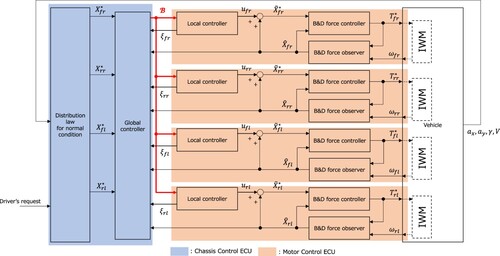
The physical functional layout of each function shown in Figure 5 is as shown in Figure 6. That is, the global controller is implemented to the chassis control ECU (ECU: Electronic Control Unit) and the local controller is implemented to the motor control ECU. As can be seen from Figure 6, the transmission signal from the chassis control ECU to the motor control ECU is $\mathcal{B}\left(t\right)$ regardless of the number of motor control ECUs, and the communication volume between ECUs can be suppressed.

Figure 6. Physical functional layout.

4. Simulation

Numerical simulations are performed to check the behavior of the control architecture constructed in Section 3.2 when the driving force of one wheel (front right wheel) or two front wheels is temporarily reduced while going straight ahead.

The following vehicle model is introduced to verify the vehicle behavior. The longitudinal motion is expressed by (19(19) $\begin{array}{rl}m\dot{V}& =X_{\mathrm{fr}}+X_{\mathrm{rr}}+X_{\mathrm{fl}}+X_{\mathrm{rl}}\end{array}$(19) ), and the lateral and rotational motions are expressed by (20(20) $\begin{array}{rl}\mathrm{mV}(\dot{\text{β}}+\gamma )& =Y_{\mathrm{fr}}+Y_{\mathrm{rr}}+Y_{\mathrm{fl}}+Y_{\mathrm{rl}}\end{array}$(20) )–(24(24) $\begin{array}{rl}{X}_d& =X_{\mathrm{fr}}+X_{\mathrm{rr}}-X_{\mathrm{fl}}-X_{\mathrm{rl}}\end{array}$(24) ), which add a moment due to the difference between the left and right braking and driving forces to a dynamic bicycle model [15]. The definitions of each variable and parameter are shown in Tables 1, 2. (19) $\begin{array}{rl}m\dot{V}& =X_{\mathrm{fr}}+X_{\mathrm{rr}}+X_{\mathrm{fl}}+X_{\mathrm{rl}}\end{array}$(19) (20) $\begin{array}{rl}\mathrm{mV}(\dot{\text{β}}+\gamma )& =Y_{\mathrm{fr}}+Y_{\mathrm{rr}}+Y_{\mathrm{fl}}+Y_{\mathrm{rl}}\end{array}$(20) (21) $\begin{array}{rl}I\dot{\gamma }& =(Y_{\mathrm{fr}}+Y_{\mathrm{fl}})l_f-(Y_{\mathrm{rr}}+Y_{\mathrm{rl}})l_r+\frac{d}{2}{X}_d\end{array}$(21) (22) $\begin{array}{rl}{Y}_{\mathrm{fr}}& =Y_{\mathrm{fl}}=-K_f(\text{β}+\frac{l_f}{V}\gamma -{\delta }_f)\end{array}$(22) (23) $\begin{array}{rl}{Y}_{\mathrm{rr}}& =Y_{\mathrm{rl}}=-K_r(\text{β}-\frac{l_r}{V}\gamma )\end{array}$(23) (24) $\begin{array}{rl}{X}_d& =X_{\mathrm{fr}}+X_{\mathrm{rr}}-X_{\mathrm{fl}}-X_{\mathrm{rl}}\end{array}$(24) In the simulations, the plant model of agent $A_{\mathrm{ij}}$ is assumed to be a first-order delay system with a time constant of 0.1 and a gain of 1 that can be expressed by the following transfer function. (25) $\begin{array}{r}{\hat{X}}_{\mathrm{ij}}\left(s\right)=\frac{1}{0.1s+1}{\tilde{X}}_{\mathrm{ij}}^{\ast }\left(s\right)\end{array}$(25) In the above model, the time constant determines the responsiveness of the agent. As discussed in Section 3.2, the controller gains $a\left(t\right)$ and $b\left(t\right)$ (especially the value of $a_0$ in the gain $a\left(t\right)$) must be adjusted according to the time constant.

Table 1. Variables.

Variable	Symbol	Unit
Body slip angle	β	rad
Yaw rate	γ	rad·s${}^{-1}$
Front wheel angle	${\delta }_f$	rad
Velocity	V	m·s${}^{-1}$
Braking and driving force	$X_{\mathrm{ij}}$	N
Cornering force	$Y_{\mathrm{ij}}$	N

Table 2. Parameters.

Parameter	Symbol	Unit
Vehicle mass	m	kg
Moment of vehicle inertia	I	kg·m${}^2$
Front tire cornering stiffness	$K_f$	N·rad${}^{-1}$
Rear tire cornering stiffness	$K_r$	N·rad${}^{-1}$
Distance from front axle to C.G.	$l_f$	m
Distance from rear axle to C.G.	$l_r$	m
Tread	d	m

First, the simulation results are shown in Figures 7 and 8 when the driving force of the front right wheel decreases to 100[N] for 2 seconds at 5 seconds after the start of the simulation while going straight ahead with a driving force of 400[N] at each wheel (i.e. $X_{\mathrm{ij}}^{\ast }$ is fixed at 400[N], $X_{+}^{\ast }=1600$[N], $X_{-}^{\ast }=0$[N]). Figure 7 shows the results without the redistribution, and Figure 8 shows the results with the redistribution by broadcast control. In both cases, the steering angle is fixed to zero (i.e. ${\delta }_f=0$[rad]) in order to confirm the influence of the drivetrain only. The initial value of vehicle speed is $V=15[\text{m}\cdot {\text{s}}^{-1}]$, and sampling time is $T_s=0.001\left[\text{s}\right]$. The parameters used during the simulation are shown in Table 3.

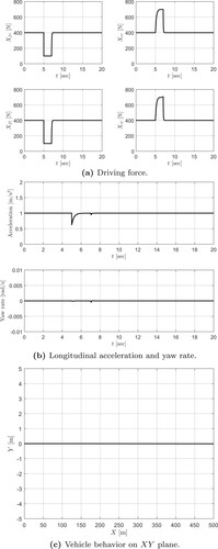
Figure 7. Simulation results of driving force reduction of front right wheel without redistribution. (a) Driving force. (b) Longitudinal acceleration and yaw rate and (c) Vehicle behavior on XY plane.

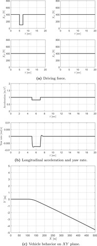
Figure 8. Simulation results of driving force reduction of front right wheel with redistribution. (a) Driving force. (b) Longitudinal acceleration and yaw rate and (c) Vehicle behavior on XY plane.

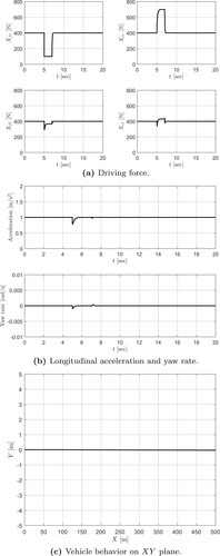
Table 3. Simulation parameters.

Symbol	Value	Unit
m	1600	kg
I	2500	kg·m${}^2$
$K_f$	55000	N·rad${}^{-1}$
$K_r$	60000	N·rad${}^{-1}$
$l_f$	1.1	m
$l_r$	1.6	m
d	1.5	m
$a_0$	0.4	–
$a_p$	0.7	–
$b_0$	0.015	–
$b_p$	0.16	–
$t_v$	100	–
$W_n$	1000	–
$W_{\mathrm{aX}}$	100	–
$W_{\mathrm{a\gamma }}$	1000	–

As shown in Figure 7(a), since there is no redistribution, the driving force of the other wheel remains at 400[N] even when the driving force of the front right wheel is reduced. As a result, the total driving force is reduced and the driving forces become unbalanced, resulting in reduced acceleration and unintended yaw rate generation, as shown in Figure 7(b). Figure 7(c) confirms that the vehicle behavior is to deviate to the right relative to the trajectory before the reduction in driving force.

On the other hand, Figure 8 shows the results for the case with the redistribution by broadcast control. As can be seen in Figure 8(a), when the driving force of the front right wheel is reduced, the total driving force and balance of left and right driving forces are maintained by the autonomous distributed operation of the other three wheels. As a result, the vehicle is able to continue going straight ahead on a trajectory that is almost the same as before the reduction in driving force, as shown in Figure 8(b,c).

Next, the simulation results are shown in Figure 9 when the driving forces of the front right and left wheels simultaneously decrease to 100[N] for 2 seconds at 5 seconds after the start of the simulation while going straight ahead with a driving force of 400[N] at each wheel (i.e. $X_{\mathrm{ij}}^{\ast }$ is fixed at 400[N], $X_{+}^{\ast }=1600$[N], $X_{-}^{\ast }=0$[N]). Other parameters and initial conditions are the same as in the simulation of the front right wheel driving force reduction. When the driving force of the front wheels decrease, the right and left rear wheels compensate for the driving force and suppress the acceleration decrease. The symmetrical operation of the rear two wheels also prevents the yaw rate caused by the imbalance between the left and right driving forces. Due to the above operation, the vehicle's trajectory does not change significantly before and after the reduction in driving force.

Figure 9. Simulation results of driving force reduction of front right and left wheels with redistribution. (a) Driving force. (b) Longitudinal acceleration and yaw rate and (c) Vehicle behavior on XY plane.

These results mean that the driver does not need to take any special action to maintain the vehicle behavior when the driving force is reduced.

In the simulation, we assumed that the front right wheel or the front two wheels lose driving force while going straight ahead, but the same behavior is confirmed for all other combinations of abnormalities that can be handled by the redundancy provided by the independent control of the four wheels (one wheel other than the front right wheel and one wheel on each side other than the front two wheels). As a result, the effectiveness of the proposed method is confirmed for all eight combinations of abnormalities described in Section 3.2.

5. Conclusion

In this study, we proposed the architecture for autonomous distributed control of braking and driving force for EVs equipped with in-wheel motors on all four wheels in the event of a wheel abnormality.

By applying broadcast control and shifting the architecture from conventional centralized control to autonomous distributed control, there is no need to prepare a distribution law for each abnormal wheel, and the control can be switched only according to the presence or absence of an abnormality, without complicated compensation rules. In addition, broadcast communication suppresses the increase in communication volume when applied to multi-wheel vehicles with an increasing number of agents to be handled. Therefore, the system is highly scalable to various abnormal scenarios and vehicle structures.

The numerical simulations have confirmed that when the driving force of one or two wheels is reduced, the vehicle behavior is maintained through the autonomous distributed behavior of the other wheels.

In the future, we plan to deepen theoretical considerations on the simulation results and design an evaluation function that includes not only the braking and driving force but also the steering angle as a decision variable to deal with a wider range of vehicle behavior. Furthermore, we try to extend the target to multi-wheeled vehicles such as lunar exploration vehicles with six wheels to verify the scalability for various vehicle structures.

Disclosure statement

No potential conflict of interest was reported by the author(s).

Additional information

Funding

This research was partly supported by JST FOREST Program #JPMJFR2123.

Notes on contributors

Akira Ito

Akira Ito received the Ph.D. degree in mechanical science and engineering from Nagoya University, Japan, in 2016. From 1998 to 2022, he worked at DENSO CORPORATION in the product design and R&D departments. From 2022 to 2024, he was an Associate Professor with the Graduate School of Engineering, Nagoya University. He is currently a Professor with the Department of Mechanical Engineering, Aichi Institute of Technology. His current research interests include vehicle control systems such as vehicle motion control, driver assistance, and autonomous driving.

Shun-ichi Azuma

Shun-ichi Azuma received his B.S. from Hiroshima University in 1999 and his M.S. and Ph.D. from the Tokyo Institute of Technology in 2001 and 2004, respectively. He was an assistant professor and associate professor at the Graduate School of Informatics, Kyoto University from 2005 to 2011 and from 2011 to 2017, respectively, and a professor at the Graduate School of Engineering, Nagoya University from 2017 to 2022. He is currently a professor at the Graduate School of Informatics, Kyoto University. He was an Associate Editor of IEEE Transactions on Control of Network Systems from 2013 to 2019, and of IEEE Control Systems Letters from 2016 to 2019. He currently serves as a Senior Editor of International Journal of Control, Automation and Systems since 2018, and as Associate Editors of IEEE CSS Conference Editorial Board since 2011, Automatica since 2014, Nonlinear Analysis: Hybrid Systems since 2017, and IEEE Transactions on Automatic Control since 2019. His research interests include analysis and control of network systems and hybrid systems.

Notes

1 The subscript i indicates f for the front wheel and r for the rear wheel, and j indicates r for the right wheel and l for the left wheel. The same meaning will be used in the following descriptions.

References

- SANEI. Passenger cars in the near future. Motor Fan Illus. 2023;200:36–41. Japanese.
- Protean Electric. Protean360+ [Internet]. United Kingdom; [cited 2023 Sep. 26] available from: https://www.proteanelectric.com/technology/#protean360plus/.
- Othaganont P, Assadian F, Auger DJ. Multi-objective optimisation for battery electric vehicle powertrain topologies. Proc Inst Mech Eng Part D J Automob Eng. 2017;231(8):1046–1065. doi: 10.1177/0954407016671275
- J MS, Harth P, Ficzere P. In-wheel-motor electric vehicles and their associated drivetrains. Int J Traffic Transp Eng. 2020;10(4):415–431.
- Azuma S, Yoshimura R, Sugie T. Broadcast control of multi-agent systems. In: Proceedings of the 50th IEEE Conference on Decision and Control and European Control Conference; 2011 Dec. 12–15; Orlando, FL, USA. p. 3590–3595.
- Ito Y, Kamal MAS, Yoshimura T, et al. On pseudo-perturbation-based broadcast control of multi-agent systems. In: Proceedings of the 2018 Annual American Control Conference; 2018 Jun. 27–29; Milwaukee, USA. p. 2877–2882.
- Ito A, Azuma S. Four-wheel independent braking and driving force control system based on broadcast control. In: Proceedings of the 66th Japan Joint Automatic Control Conference; 2023 Oct. 7–8; Sendai, Japan. Japanese.
- Yoshimura M, Fujimoto H. Driving torque control method for electric vehicle with in-wheel motors. Electr Eng Japan. 2012;181(3):49–58. doi: 10.1002/eej.v181.3
- Johansen TA, Fossen TI. Control allocation—a survey. Automatica. 2013;49:1087–1103. doi: 10.1016/j.automatica.2013.01.035
- Mokhiamar O, Abe M. Effects of an optimum cooperative chassis control from the viewpoint of tire workload. Trans Soc Autom Eng Japan. 2004;35(3):215–221.
- Zhang H, Liang H, Tao X, et al. Driving force distribution and control for maneuverability and stability of a 6WD skid-steering EUGV with independent drive motors. Appl Sci. 2021;11(3):961. doi: 10.3390/app11030961
- Wang Y, Fujimoto H, Hara S. Torque distributed-base range extension control system for longitudinal motion of electric vehicles by LTI modeling with generalized frequency variable. IEEE Trans Mechatron. 2016;21:443–452.
- Ito A, Hanamoto K, Ichinose S. Vehicle motion planning and control with road geography information for energy reduction. In: Proceedings of the 15th International Symposium on Advanced Vehicle Control; 2022 Sep. 12–16, Yokohama, Japan.
- Maeda K, Fujimoto H, Hori Y. Front and rear driving force distribution method for retaining driving force on instantaneous slippery roads for electric vehicle with in-wheel motors. Trans JSME. 2012;78(794):53–62. Japanese
- Ito A, Hayakawa Y. Design of a fault tolerant robust control system for a vehicle with steer-by-wire and in-wheel motors by utilizing steering and drive-train systems. Trans Soc Instrum Control Eng. 2014;50(11):801–810. doi: 10.9746/sicetr.50.801. Japanese.
- Gáspár P, Bokor J, Mihály A, et al. Robust reconfigurable control for in-wheel electric vehicles. IFAC-PapersOnLine. 2015;48(21):36–41. doi: 10.1016/j.ifacol.2015.09.501