Estimating Pedestrian Flows on Street Networks

Abstract

Problem, research strategy, and findings

City governments and planners alike commonly seek to increase pedestrian activity on city streets as part of broader sustainability, community building, and economic development strategies. Though walkability has received ample attention in planning literature, most planners still lack practical methods for predicting how development proposals could affect pedestrian activity on specific streets or public spaces at different times of the day. Cities typically require traffic impact assessments (TIAs) but not pedestrian impact assessments. In this study I present a methodology for estimating pedestrian trip generation and distribution between detailed origins and destinations in both existing and proposed built environments. Using the betweenness index from network analysis, I introduce a number of methodological improvements that allow the index to model pedestrian trips with parameters and constraints to account for pedestrian behavior in different settings. I demonstrate its application in the Kendall Square area of Cambridge (MA), where estimated foot traffic is compared during lunch and evening peak periods with observed pedestrian counts.

Takeaway for practice

The proposed approach can be particularly useful for TIAs, neighborhood plans, and large-scale development projects, where pedestrian flow estimates can be used to guide pedestrian infrastructure and safety improvements and public space investments or for locating pedestrian priority streets during the COVID-19 pandemic.

Keywords:

• betweenness
• pedestrian mobility
• route assignment
• trip distribution
• trip generation

Pedestrian activity on city streets constitutes a powerful indicator of the social, environmental, and economic health of a community. A high level of pedestrian activity is often associated with more sustainable urban form (Gehl, 2010; Speck, 2013), robust local economies (Glaeser, 2010), better public health outcomes (Forsyth et al., 2008; Oishi et al., 2015; Rundle et al., 2007), and stronger social networks (Rogers et al., 2011). A lack of pedestrian activity, on the other hand, signals built environments that fail to offer origins and destinations within walking range or that compromise basic safety, comfort, and stimulation standards necessary to bring people out on foot.

Yet relatively little work in both planning and transportation fields has focused on modeling and predicting pedestrian flows along city streets (Transportation Research Board [TRB], 2014b). Unlike vehicular traffic impact assessments (TIAs), which are widely used in planning practice and are, in fact, required by municipalities for development review, it is extremely rare to encounter methods for projecting changes to pedestrian flow as part of project impact analysis. This difference is consequential; numeric and spatial results matter. If vehicular TIAs demonstrate that additional projected traffic from a development is likely going to diminish level of service (LOS) on particular road segments or intersections, municipal regulations commonly require mitigation measures to be implemented, such as road widening, additional turning lanes, traffic light adjustments, or parking.¹ As a result, most transport investments are funneled to capital intensive vehicular infrastructure, not pedestrian infrastructure, where equivalent traffic science and legal frameworks remain absent. For cities to enhance walking, it is important to estimate not only how many total walking trips a planned area might generate but how these trips are likely to distribute along specific streets. Unlike vehicle TIAs, which generally aim to minimize additional vehicle miles traveled, pedestrian TIAs could aim to increase pedestrian activity. To move toward this aim, readily accessible tools are needed to estimate how proposed site plans, neighborhood plans, and zoning changes could contribute to pedestrian activity on streets and public spaces.

Here I present a network-based pedestrian flow model that moves beyond simple approximations to estimate specific time-of-day pedestrian flows between origins and destinations in dense urban environments. This can help guide both developer contributions and city investments into better walking conditions: where to widen sidewalks or implement curb extensions; where to invest in better pavers, street furniture, or lighting; where to implement safe crossings; or where to zone for commercial ground-floor activities. The methodology can be applied to a number of planning scenarios that require forecasting local-level pedestrian travel demand: competitive funding applications to metropolitan planning organizations (MPOs) and state or federal agencies for pedestrian improvement projects; nonmotorized mobility impact assessments of comprehensive plans, neighborhood plans, or urban design projects; and TIAs of individual development projects in high-density areas. In light of the COVID-19 pandemic, it can further support municipal efforts in identifying the most beneficial locations for “shared streets” initiatives to enable safe outdoor pedestrian interaction.

In the literature review I discuss common approaches to analyzing walkability impacts, placing the proposed approach in a practical context. In the following section I describe the proposed model. I then illustrate how it can be calibrated using Kendall Square in Cambridge (MA) as an example, where I compare predicted footfall on around 60 street segments to actual footfall during lunch and evening peak periods. Finally, I illustrate how the present levels of foot traffic in the same study area could change as a result of development activity that is currently taking place in the area. In the last section I discuss improvements and opportunities for using pedestrian flow models in planning practice.

Literature and Practice

The National Cooperative Highway Research Program has produced a number of reference reports on the current practice on travel forecasting and active transportation travel forecasting in particular (TRB, 2012, 2014a, 2014b, 2014c, 2016). At the regional level, travel forecasting is most commonly accomplished through travel demand models (TDMs), which provide long-term forecasts and are mostly operated by MPOs and large cities.² At the local scale, short-range, nonmotorized travel demand forecasting is typically achieved through “sketch planning” and “factoring methods” (U.S. Department of Transportation [DOT], Federal Highway Administration, 1999). Sketch planning can approximate pedestrian demand based on simple comparative analysis of locations and rules of thumb. This typically involves regressing observed pedestrian counts against land use mix, density, or other built environment variables and applying regression coefficients to predict pedestrian activity in a comparable area (Matlick, 1996). In practice, consultants often use journey-to-work mode share estimates from the American Community Survey (ACS) to obtain approximate pedestrian mode share (Aoun et al., 2015). Since 2016, the Institute of Transportation Engineers (ITE) has also published peak-period person trip generation rates (as opposed to only vehicular trip generation) for different land use types, which also have been used in practice to evaluate pedestrian demand or to forecast change in pedestrian activity in new projects (ITE, 2016; Weinberger et al., 2014). However, both ACS journey-to-work data and ITE trip generation tables are coarse and often insufficient for pedestrian impact assessment of specific projects: ITE trip generation rates, which are largely based on suburban data, depend little on specific context³ and offer “average” estimates to describe how many trips different land use categories generate during peak travel periods (Weinberger et al., 2014). Moreover, trip rates are uniquely based on origin land use types, ignoring destination availability, and they are also not spatialized: they do not suggest where and how much activity would flow through street segments or intersections. ACS nonmotorized journey-to-work data, on the other hand, are often so sparse that they have no statistical significance even in dense urban areas (Kantz, 2020).

If TIA consultants spatialize projected pedestrian activity around a site, they typically indicate primary walking routes to surrounding amenities (e.g., transit, schools, shops) based on their intuition. Unlike vehicular TIAs, which are calibrated on counts and modeled on networks, pedestrian movement, if included at all, is regarded as “soft,” subjective, and imprecise. Much of the theoretical and academic work on walkability also stands on aggregate relationships between built environment and walking activity, without spatializing the flow of pedestrians between particular origins and destinations along specific routes people prefer to take (Ewing & Handy, 2009; Ewing et al., 2006; Lee & Talen, 2014; Talen, 2003).

Pedestrian movement has been spatially distributed in agent-based simulations that generate movements of individual people (agents) based on origin–destination pairs and a set of behavioral assumptions (Batty, 2003; PTV, 2008). Such simulations can offer high-resolution results where each individual trip is spatially visualized. But a high degree of specificity and extensive setup requirements have also limited the applicability of agent-based pedestrian models to fairly small sites, such as airports, transit stations, or a few downtown blocks (Puusepp et al., 2017).

Pedestrian trajectories have also been analyzed by route choice researchers using discrete choice models. Such studies found pedestrians prefer routes that are safer (Agrawal et al., 2008; Broach & Dill, 2015; Tribby et al., 2017), more comfortable (Erath et al., 2015; Greenwald & Boarnet, 2001), and more interesting (Guo, 2009, Guo & Loo, 2013; Lue & Miller, 2019) or that are cognitively simpler to navigate, minimizing turns or maximizing landmarks and other navigational aids along the way (Golledge, 1995; Lue & Miller, 2019; Shatu et al., 2019). However, rarely have pedestrian route choice findings been applied to predict the spatial distribution of pedestrian flows that could result from different urban development alternatives. Cooper et al.’s (2019) prediction of longitudinal effects of downtown redevelopment on pedestrian flows in Cardiff (Wales) using a network analysis approach offers a recent and promising exception.

Pedestrian flow prediction has emerged in network-based models, such as PedContext, MoPed, Urban Network Analysis toolbox, sDNA, Depthmap, Urbano, and MCA, which estimate individual-level pedestrian movement trajectories but do so mathematically, without visualizing individual agents’ journeys (Allen et al., 2004; Clifton et al., 2016; Cooper & Chiaradia, 2020; Crucitti et al., 2006; Dogan et al., 2018; Porta et al., 2006; Sevtsuk, 2018; Sevtsuk & Kalvo, 2021; Turner, 2001). Instead, the number of trips traversing each network link is estimated using graph theory methods, computing results much faster and for significantly larger study areas than agent-based approaches. This makes network analysis an attractive option for planners and urban transportation consultants, whose neighborhood-scale work stands to particularly benefit from their use (Crucitti et al., 2006; Kazerani & Winter, 2009; Sevtsuk & Mekonnen, 2012; Ye et al., 2016). Here I also focus on network-based pedestrian flow estimation and propose several improvements and innovations over existing techniques.

The approach I use to model pedestrian flows over networks is based on the “betweenness” algorithm. One of the earliest examples of using network analysis to model pedestrian flows was provided by Garbrecht (1971), who investigated the distribution of walking trips in uniform grids.⁴ Freeman (1977) is usually credited as first to formalize the betweenness algorithm for social network analysis, which many subsequent authors have used for trip modeling over spatial networks. A thorough review of these variants is provided by Brandes (2008). Hillier and Iida (2005), Allen et al. (2004), Porta et al. (2009, 2012), Sevtsuk (2014), and Cooper et al. (2019), among others, have demonstrated how betweenness can be applied to estimate movement on street networks. These studies have shown that the betweenness algorithm holds great potential not only for explaining pedestrian activity in existing built environments but also in predicting pedestrian activity in new development plans.

Proposed Model

Traditional betweenness centrality of a node in a network is defined as the number of shortest paths between all other node pairs in the network that pass through that node (Freeman, 1977). If more than one shortest path is found between two surrounding nodes, then each equidistant path is given equal weight (see Technical Appendix 1). Given a set of trip origins and destinations, the index colloquially captures the flow—or in this case the foot traffic—that passes through each network segment or node.

Applying the conventional betweenness index to estimate pedestrian flow on street networks requires several adjustments. First, instead of measuring trips between all nodes in a network, as is common in social networks, the approach below enables the model to capture trips between separate origins and destinations. This allows betweenness results to be estimated from homes to transit stations, for instance (Garbrecht, 1971).

Second, similar to other local area network analysis approaches (Hillier & Iida, 2005), a search radius variable is implemented, which enables users to determine the maximum network distance between origins and destinations for which trips are modeled. A search radius constraint allows trips from homes to transit stations, for instance, to be limited to only those homes that are up to a certain distance from their nearest station.

Third, a detour ratio variable is added, which enables trips between origin–destination pairs to be routed along all “plausible” paths that are up to a certain percentage longer than the shortest path. Different versions of this adjustments have been proposed by Allen et al. 2004, Jiang (2009), Bavaud and Guex (2012), Kivimäki et al. (2016), and Cooper et al (2019). Detour ratio here describes the ratio between the allowable path length and the shortest path length between a node pair. A detour ratio of 1.15, for instance, will tell the algorithm to find all paths that are up to 15% longer than the shortest path between given origin–destination pairs. The total number of trips starting from an origin is split, with equal probability between each “plausible” path found and the betweenness values of individual path segments are cumulatively summed.

Fourth, the number of trips starting at each origin point is controlled by an origin node weight (W). Whereas in social networks it is common to measure betweenness by routing one trip from each node to each other node in the network, different origins in urban settings emit different numbers of trips. A high-rise building with more office workers will generate more trips to a transit station than a single-family home in a similar context. The origin weights here are analogous to baseline ITE trip generation rates, but they go through a calibration process to arrive at locally specific rates used in the model.

Fifth, a destination elasticity term is added to the betweenness algorithm, which adjusts the probability of pedestrian trips based on destination weights and distances.⁵ Surveys have shown that shorter walking trips are exponentially more likely than longer trips to the same destination. This fundamental feature of geography (Hansen, 1959; Liang et al., 2013; Tobler, 1970) is typically missing from the application of the betweenness index to social networks, but it is an important factor in spatial networks (Gao et al., 2013). The model has a gravity accessibility function, which ensures that nearer destinations or more attractive destinations (those with larger weights) receive more trips. Similar to Handy and Niemeier (1997), it includes an exponential distance decay with a coefficient (beta) to adjust walking probabilities with respect to distance (see Technical Appendices 2 and 6). The effect of destination attractiveness on trip rates is controlled by an exponent alpha.

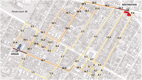
These five adjustments produce a modified betweenness index specifically for estimating walking trips (Technical Appendix 3). Figure 1 illustrates the results of the index between one origin–destination pair using a detour ratio of 1.2, which finds all routes that are up to 20% longer than the shortest path. Fifty-six unique routes were found in this case. Because the origin point has a weight of 100 and is located 290 m from a destination (destination not weighted), instead of routing all 100 trips to the destination, only 75 trips are sent out, assuming a distance decay coefficient of 0.001.⁶ Given that all 75 trips must cross the street segments in front of the origin and destination points, the betweenness values of both of these segments are 75. Other segments along the way obtain lower values depending on how many of the 56 “plausible” routes pass by them.⁷

Figure 1. Betweenness results for street segments for a single origin–destination pair, where the origin has a weight of 100 (of which only 75 are routed due to a distance decay effect) along all routes that are up to 20% longer than the shortest path.

Finally, the sixth adjustment concerns situations that involve multiple competing destinations. When allocating trips from workplaces to eateries during the lunch period, for instance, it is typically unclear which particular eatery each pedestrian might prefer. Instead of oversimplifying the analysis and allocating the trip to only the closest eatery or, alternatively, repeating the same number of trips to each eatery, betweenness estimation is combined with a modified version of Huff’s choice model, which assigns probabilities to competing destinations based on their accessibility (Huff, 1963).

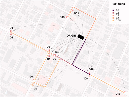
However, differing from Huff’s original approach, the model here does not assume that 100% of origin point weights are allocated between the competing destinations. Instead, after assigning a probability to each destination, the model allocates trips based on both the proximity and attractiveness of the destinations⁸ (see detailed specification in Technical Appendix 4). Figure 2 illustrates this concept with an origin point that produces a single trip, which is split between 13 competing destinations (bus stops in this case). A fraction of walking trips from the origin is sent to each of the available bus stops, but those that are closer or more attractive get a larger share. For instance, I have allocated destination D10 a larger weight than other stops (i.e., bus stop serves more lines), which results in more trips to D10 as well as those stops that are closer to the origin.

Figure 2. Betweenness patronage analysis allocates a fraction of trips from the origin to each of the competing destinations found within a given network radius, based on the gravity accessibility of destinations. In this example, D10 has the largest weight and attracts most trips.

In addition to distributing trips spatially, the model can estimate the total patronage volume at each destination. Multiplying these patronage volumes with corresponding regression coefficients and summing across all destinations produces a total pedestrian trip volume in a study area for a given time period. This can be used for explaining how many total walking trips an area generates or how much change in walking trips may result from redevelopment.

Both trip generation and distribution can change as a result of adding new origins: If a residential building is developed, it can generate new trips to surrounding destinations. Trip generation and distribution also depend on destinations: Enlarging a park, all else equal, not only redistributes trips from existing parks but also generates some new trips due to the added size effect. The same park can also act as an origin for trip generation.

In terms of mode choice, the model only includes one travel mode at a time—walking, though it can also be calibrated for biking—which is enforced by using a trip cutoff distance (e.g., 1,500 m) and a distance decay rate specific to pedestrians (Technical Appendix 6). If origin points do not have any destinations within a given distance, or if the destinations are relatively far or small, then few or no pedestrian trips may be estimated to the given destinations. This does not mean that people at the given origins are unable to access such destinations at all—they are simply assumed to be unable to access them on foot and may instead resort to other travel modes that are not incorporated in this model. Conversely, if a redevelopment project generates additional pedestrian origins and destinations, it is assumed that newly generated walking trips come in part because of a modal shift (e.g., replacing vehicular trips that would have gone to destinations further away) and in part as newly induced trips that did not exist before.

The software implementation enables planners and transportation analysts to model thousands of trips between various origin–destination pairs simultaneously. This enables pedestrian flows to be both examined in existing environments and forecasted as part of a future planning scenarios. Though somewhat analogous approaches have been used for flow modeling before (Allen, 2004; Cooper et al., 2019; Gao et al., 2013; Ye et al., 2016), I am not aware of prior uses of the betweenness algorithm for walking behavior that combine it with probabilistic destination choice and exhaustive alternative route generation as part of a relatively easy-to-use software tool.

Case Study Application: Estimating Pedestrian Flows Around Kendall Square

I implemented the proposed model to analyze pedestrian flows around Kendall Square in Cambridge. Kendall Square is located on the Massachusetts Institute of Technology (MIT) campus, surrounded by mixed-use office, laboratory, and hotel buildings in addition to MIT facilities (Figure 3) and a subway station, which attracts roughly 1,700 boardings during the 12 p.m. to 2 p.m. lunch period and 8,500 boardings during the 4 p.m. to 8 p.m. evening peak period (Massachusetts Bay Transportation Authority [MBTA], 2020). Aside from a few high-end apartment structures and a couple of MIT dormitories, housing is scarce in the immediate vicinity of the Kendall station. The heart of Kendall Square is instead home to a significant high-tech office cluster, which commands the highest per-square-foot office leases in the greater Boston area. More than 300 biotechnology companies and major information technology firms like Google and Microsoft have offices at Kendall. According to the U.S. Census and Esri ArcGIS Business Analyst 2015 data, 23,454 residents and 80,250 jobs were located in a 15-min (1,500 m) walkshed around the Kendall T station (Esri, 2015; U.S. Census Bureau, 2015a). The median household income in the same walkshed was $99,302 per year. Pedestrian flows around Kendall are therefore dominated not only by students and university employees but also by a mix of office, lab, service sector, and custodial workers as well as visitors who frequent the area daily.

Figure 3. Kendall Square study area.

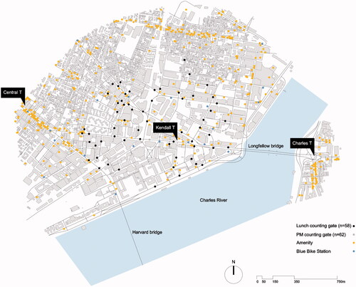
Pedestrian counts around Kendall Square were performed during two separate periods: workday lunch period (12–2 p.m.) and evening peak travel period (4–8 p.m.) in October 2018 during clear weather. Observers were positioned for 20-min counting windows at 60 preselected counting locations during the evening peak period and 58 locations during the lunch period (Figure 3).⁹ Counts were subsequently aggregated upwards to represent the full duration of the lunch and evening peak periods. Counting locations were chosen as a stratified sample to include street segments that were expected to have high, medium, and low levels of foot traffic and to ensure broad geographic coverage within the 1.5-km walkshed around the T station, not only the primary streets near the station itself.

The average bidirectional pedestrian flow on both sides of the street across all counting locations was 872 pedestrians during the lunch period and 1,711 during the evening period. A maximum flow of 11,311 pedestrians was observed on Main Street, right in front of the Kendall T station, during the evening peak.

Model Setup

To set up a comprehensive origin–destination network, 2014 TIGER/Line (Topologically Integrated Geographic Encoding and Referencing) centerlines of Cambridge streets were used to construct a spatial network. All building centroids within a 15-min (1,500 m) walkshed of the T station were included as potential trip origins (Figure 3). Each building was given a set of numeric weights according to the estimated number of residents, jobs, students, or amenities it contained. To achieve a more granular estimation, census block–level residential counts were interpolated to individual residential buildings, weighted by the gross floor area of the building. Larger residential buildings thus obtained a proportionately larger share of the block’s population, whereas the overall count in the block stayed identical to the original census numbers. Employment counts were directly available at the building address from Esri Business Analyst.

I also used Esri Business Analyst data to locate all eating and drinking places, retailers, personal services, nightlife, art and entertainment venues, and schools in the area. Subway stations and bus stop locations were obtained from the MBTA via MassGIS (MBTA, 2017) and shared bike dock locations were obtained from Bluebikes (n.d.). The locations and sizes of parks, playgrounds, and greenspaces were obtained from the City of Cambridge (2020). Taken together, these locations provide 56 potential origin–destination pairs for pedestrian trips (Technical Appendix 5).

Rather than exhaustively modeling flows between each of the possible origin–destination pairs, I expected a few key pairs to dominate the overall pattern of pedestrian traffic during both periods. For instance, although some walking trips from homes to parks do take place during the lunch period, they are probably not the most common trip type. Given the high density of office space, proximity to MIT, and the presence of a subway station, workplace-to-restaurant and workplace-to-subway trips were expected to be more common during lunch. To test numerous options, I modeled trips between a number of reasonable origin–destination pairs (highlighted in gray in Technical Appendix 5).

To choose an appropriate distance decay (β) coefficient for routing trips from origins to destinations at various distances (see Technical Appendices 2 and 3), several beta values were tested in the model and 0.001 (in meters as units) was identified as the best-fitting value across lunch and evening period flows (Technical Appendix 6). I used this value in specifying all origin–destination flows in the model. The destination attractiveness coefficient alpha was not needed here because destinations were not weighted in this application (see Technical Appendix 7).

For the detour ratio, I used a value of 1.15 to enable the betweenness index to find all routes that are up to 15% longer than shortest paths. This was informed by previous pedestrian route choice literature that has found people commonly choose routes that are 10% to 20% longer than shortest paths (Li & Tsukaguchi, 2005; Takeuchi, 1977; Zacharias, 2001), even up to 55% (Vanky, 2017).

Model Calibration With Observed Pedestrian Counts

Estimated flows are adjusted with coefficients, which are determined with regressions, similar to Cooper et al. (2019). Modeled flows can over- or underestimate actual trips when the same origin weights are used to generate trips to multiple sets of destinations. Regressing these against observed pedestrian counts allows us to adjust the flows to realistic levels.

Model 1 in Table 1 is an ordinary least squares (OLS) regression with eight independent origin–destination flows, with the observed evening pedestrian counts as the dependent variable. Pearson’s correlations in the second column indicate that all origin–destination trips except “residents-to–bus stops” were individually correlated with the observed pedestrian flows. Some origin–destination pairs fail to show a significant controlled effect, but workplace-to-subway, workplace-to–eating establishments, amenities-to-amenities, and Bluebikes stations–to-subway trips are statistically significant. By necessity, the individual origin–destination flows tend to be collinear because many of them originate from or flow toward the same locations over a limited street network. The second model reduced the number of variables down to four, including only workplace-to-subway and workplace-to-bus, amenities-to-amenities, and Bluebikes stations–to-subway trips,¹⁰ without a significant drop in the model fit.¹¹

Table 1 Evening peak period, 4 p.m. to 8 p.m. (n = 58). OLS estimates for evening-peak pedestrian flows.

Average: 1,711
Min: 0
Max: 11,311
SD: 2,168
	Corr.	Model 1		Model 2		Model 3		Model 3
Origin → Destination variable	alone	OLS		OLS		OLS		VIF
Employees/students → Subway	0.79	0.43*	(1.70)	0.31^ψ	(1.39)	0.73***	(7.72)	1.58
Employees/students → Bus stops	0.42	−0.99^ψ	(−1.52)	0.13	(0.33)
Employees/students → Food and beverage	0.54	0.83**	(2.12)
Amenities → Amenities	0.68	146.63*	(1.75)	245.27***	(7.73)	248.70***	(7.60)	1.58
Amenities → Subway	0.84	−26.57	(−0.34)
Bluebikes stations → Subway	0.85	2,425.92***	(2.52)	1,639.12**	(2.39)
Residents → Subway	0.75	−0.51	(−0.45)
Residents → Bus stops	−0.06	0.41	(0.06)
Adjusted R^2		0.85		0.84		0.83
F-statistic		42.78		80.98		149.10

The third model only includes two types of flows, which appear to be key to explaining evening peak hour foot traffic in the Kendall area: trips from workplaces to subway and trips from amenities to other amenities, which capture footfall between storefronts on streets. These two flows alone explain 83% of the variation in foot traffic in the area. Trips from workplaces were weighted by the corresponding number of employees and students at each origin building (Technical Appendix 7 provides weight details). The coefficient 0.729 suggests that, on average, 73% of employees and MIT students in the study area could be walking to the Kendall T station during the evening peak hour. Rosenfield (2018) finds that 56% of MIT staff use transit to commute to work. Given that my sample includes MIT students in addition to staff, who have less access to cars, and that most jobs in my study area closer to the T station than an average MIT office, a higher share is expected.

Trips from amenities to other amenities were not weighted; instead, a single trip was sent out from each amenity, a fraction of it going to each of the other amenities around it within a 1-km radius. The coefficient suggests that, on average, 248.7 visits arrived at commercial amenities from other like amenities in the area during the evening peak period (4–8 p.m.). Variance inflation factors (VIFs) shown in the table suggest that moderate correlation is found among the final variables (VIF < 5) but not severe enough to warrant corrective measures. Overall, the two origin–destination flows in evening peak model 3 explain 83% of the variation observed in pedestrian counts.

A separate set of three models was estimated for the lunch period between 12 p.m. and 2 p.m. (Table 2). Similar to the evening peak flows, correlations were first tested alone between each origin–destination flow and the observed pedestrian counts at lunch (column 2); based on this, successive regressions were tested with a different set of origin–destination pairs (columns 3–5). Dropping variables from models 1 and 2 did not reduce the R² fit. Model 3 offers a reduced setup, where pedestrian flows during lunch are related to three types of trips: 1) workplaces to eating/drinking establishments, 2) amenities to amenities (foot traffic between storefronts), and 3) subway to amenities. These three flows explain 77% of the variation in observed lunch period pedestrian counts.

The first coefficient in model 3 suggests that 42% of workers and students walk to eating and drinking establishments during lunch. The amenities-to-amenities pedestrian flow coefficient suggests that, on average, 49 visits to a typical store arrive from other stores in the area during the lunch period. The third coefficient suggests that an average restaurant attracts 34 visitors from a subway station for lunch. It is important to note, however, that this inference can only be interpreted suggestively because it is not directly observed at any of the restaurants or subway stops but is simply drawn on the basis of correlations between the three estimated origin–destination flows and the observed pedestrian counts on 58 streets. About a quarter of variation in observed pedestrian counts also remains unexplained by the model.

Table 2 Lunch period, 12 p.m. to 2 p.m. (n = 62). OLS estimates for lunch-period pedestrian flows.

Average: 873
Min: 48
Max: 4,066
SD: 873
	Corr.	Model 1		Model 2		Model 3		Model 3
Origin → Destination variable	alone	OLS		OLS		OLS		VIF
Employees/students → Subway	0.57	0.05	(0.51)
Employees/students → Food and beverage	0.62	0.62***	(3.22)	0.52***	(3.42)	0.42***	(3.77)	3.27
Employees/students → Parks	0.45	−0.04	(−0.17)	−0.18	(−0.98)
Amenities → Amenities	0.61	51.37^ψ	(1.37)	47.53*	(1.61)	48.83*	(1.66)	4.22
Amenities → Subway	0.67	−16.13	(−0.44)	36.49***	(3.57)	33.97***	(3.44)	2.08
Employees/students → Blueikes stations	0.37	−0.74^ψ	(−1.24)
Bluebikes stations → Subway	0.65	787.60^ψ	(1.50)
Adjusted R^2		0.77		0.77		0.77
F-statistic		27.38		47.06		62.47

Notes: Cell entries are coefficients, with t-statistics in parentheses. Variable weights, beta values, search radii, and detour ratios are shown in the Technical Appendix.

^ψp < .25; *p < .1; **p < .05; ***p < .01.

In summary, relatively few origin–destination flows explain a relatively high share of variation in the observed foot traffic around Kendall Square during both evening peak (R² = 0.83) and lunch (R² = 0.77). Collinearity between individual flows was likely canceling out some of the controlled effects in the OLS model I used. Collinearity can be further addressed in future work using estimation techniques designed to address overlapping variables, such as by combining variables, using ridge regressions, or machine learning models, which can additionally address nonlinear relationships.

Predicting New Development Impacts

Given the calibration on observed pedestrian counts in an existing built environment, could the model be extended to predict change in foot traffic that may result from new developments in the area? Kendall Square is a rapidly developing part of Boston, with multiple major construction projects under way. Close to half a million square meters of new floor area (4.58 million gross square feet) is being developed around Kendall at present, which will add 16,183 new jobs and 3,600 new residents to the study area within the next couple of years (Cambridge Redevelopment Authority, 2018; MIT, 2018).

To explore such prediction, I took the origin–destination coefficients from the final evening peak model and estimated foot traffic on each street segment in the area before and after redevelopment. I included two types of origin–destination trips in the prediction—workplace-to-subway trips and amenities-to-amenities trips—as defined in model 3 of Table 1. Gross floor areas (GFAs) and residential units associated with redevelopment under way were obtained from the City of Cambridge directly. The number of employees and the number and location of amenities had to be estimated based on the GFA and use mix of each new building. To approximate jobs, I estimated 60 m² per job in new commercial properties (U.S. Energy Information Administration, 2016). For amenities, I used the presently observed ratio of GFA to amenities in the whole study area to add amenities on ground floors of new developments.

Figure 4 illustrates the projected change in pedestrian flows. Higher levels of change in footfall are symbolized with thicker lines and labeled next to each street segment. As expected, the highest increase in foot traffic occurs on streets that face new developments and streets that lead from new developments to subway stations or surrounding amenities. The greatest addition of pedestrian flow takes place in front of the Kendall T station near the corner of Third Street, where the evening peak foot traffic is projected to increase by 55% over current conditions (from 7,155 pedestrians to 11,126 pedestrians).

Figure 4. Estimated change in foot traffic around Kendall Square due to redevelopment. Values indicate increase or decrease in pedestrians during the evening peak period (4–8 p.m.).

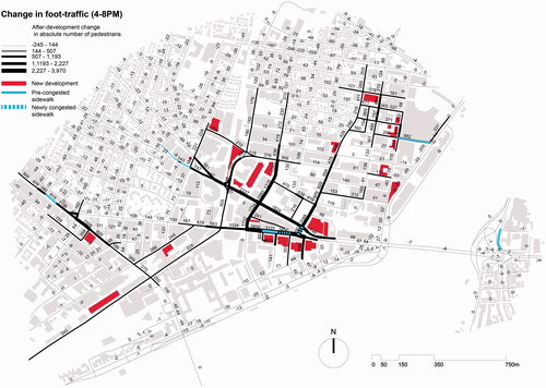
Note that because of the nature of the destination choice model, change in pedestrian flow that results from new development does not necessarily have to be positive on each street segment. For workplace-to-subway trips, new development can only increase foot traffic, because the set of destinations (subway stops) remain unchanged while new employment locations add new origins. However, negative change can occur when newly established ground-floor amenities shift destination probabilities of existing trips toward new destinations, reducing trips around previous amenity locations. Indeed, the legend in Figure 4 shows that the predicted change in footfall ranges from −245 to +3,970 pedestrians during the evening period.

In terms of pedestrian trip volume, the model estimates that before redevelopment there were a total of 180,427 movements in the study area during the 4-h evening peak period, which includes three subway stations (Kendall Square, Central Square, Massachusetts General Hospital) and a number of commercial clusters shown in Figure 3. As a result of redevelopment, this volume is expected to rise by 22,581 additional pedestrian trips (6,491 new trips to subway and 16,090 new movements between amenities). Of all of the newly generated trips to the subway, 5,230 are estimated to head to Kendall Station, 871 to Central Station, and 390 to Massachusetts General Hospital Station.

As an example of how these results can be used to examine the impacts on pedestrian LOS, estimated flows on individual streets can be compared with known sidewalk dimensions to highlight segments where pedestrian congestion could occur. Gehl Architects’ studies from around the world suggest that the maximum volume for comfortable pedestrian movement is around 12 people per minute per yard of sidewalk width: Exceeding this level is considered overcrowded (New York City DOT, 2008). Adjusting the estimates shown in Figure 4 to per minute flows and comparing them to sidewalk dimensions in Cambridge, I have highlighted seven street segments in solid lines, where pedestrian congestion was observed already before redevelopment, and two additional segments in dashes where pedestrian congestion is likely to occur as a result of examined redevelopments during workday evening hours. The analysis results could also be used to improve pedestrian safety or comfort by informing which intersections might require enhancements or to evaluate how a new through-block pedestrian link could alter pedestrian flows or affect specific sidewalk activities like street vending (Loukaitou-Sideris 2011). The model could inform whether developer contributions to improving the pedestrian realm that come from TIA recommendations may be better spent on immediate streets fronting the development or enhancing problematic intersections on nearby streets.

Use of Pedestrian Impact Assessments in Planning

In this study I introduce a methodology that can be used to estimate foot traffic on street networks at different times of day. Instead of using sketch planning coefficients, ACS travel-to-work modal share estimates, or static travel demand tables that project pedestrian trip volumes from origin points in new developments, my proposed model considers pedestrian flows between origin–destination pairs and provides a spatial foot traffic estimate for every street segment. Building on previous work, the model includes several updates that customize the betweenness algorithm for pedestrian behavior and shows how origin–destination flow rates can be empirically calibrated for different times of the day with pedestrian counts. It is implemented and available as part of the free Urban Network Analysis plugin for Rhinoceros software (Sevtsuk, 2018).

The model offers one possible approach for estimating development-induced pedestrian impacts, analogous to how vehicular traffic has been modeled as part of TDMs. How could this be implemented in practice? Although a customized pedestrian calibration survey could be appropriate in some cases (e.g., neighborhood redevelopment, Main Street plans), it would be unrealistic for planners, developers, and their transportation consultants to implement all aspects of the model in a typical development TIA: document origin–destination pairs, use these to run the flow model, calibrate the flow model with observed counts, and rerun the model with the proposed GFAs added to existing conditions to forecast spatial change in foot traffic. It would be more practical for a municipality to establish and maintain either a citywide or a districtwide (e.g., central business district, other subcenter districts) pedestrian flow model that is calibrated every couple of years with new pedestrian counts. The model could be set up and calibrated by a consultant or trained city staff and have a browser-based interface that automatically assesses the estimated change in foot traffic when land use densities are modified, mapping out the projected morning, afternoon, and lunch period impacts on individual streets, public spaces, and intersections. In contrast to TDMs used by MPOs and large municipalities already, a city- or districtwide pedestrian flow model would focus on forecasting short-term impacts of development change, which is substantially easier to set up, calibrate, and maintain. Because a municipal model could estimate current pedestrian volume on all streets in a district (not only those where calibration counts are collected), it could also establish a valuable resource for active transportation consultants.

Among possible use cases, I outline three potential scenarios in the following. First, TIAs of individual development projects in relatively dense and walkable urban areas could require applicants to use the model to determine project impacts on pedestrian flows in the surrounding area. Applicants plug in project numbers and locations—GFA of each use type, main entrance locations—to a city-maintained web interface that evaluates pedestrian volumes and flow distribution on surrounding streets. Modifications negotiated between the city and developer can be examined by updating the numbers. Similar to vehicular LOS analysis, analysis results can inform where enhancements to pedestrian facilities are needed—which intersections warrant safer crossings, which street segments need better sidewalks, curb extensions, street furniture, or lighting—to guarantee a high level of pedestrian LOS around each site.

Second, the model could also be used as part of earlier-stage neighborhood planning to determine how considered zoning changes, upcoming urban design projects, or public space improvements could affect, and desirably benefit, pedestrian activities. Estimated pedestrian flow numbers throughout the whole planned area can shed light on the viability of retail and service businesses at different locations or provide feedback to planners on where additional densities or land use mixes could increase foot traffic to levels needed to support desired amenities or activities. The results can also be incorporated into cost–benefit analyses of specific pedestrian infrastructure and public space investments contained in a bigger plan (e.g., street upgrading, safe crossings), which state and federal funding sources require already.

It is not necessary to deploy all of the steps described in the Kendall example above. Planners might only be interested in examining the quality of critical routes to a single destination (e.g., a park) or between specific origin–destination pairs (routes between homes and playgrounds), which do not necessarily require impact analysis of future projects.

Third, medium- and large-scale developers could use the model to analyze frontage value or to inform how project massing, use distribution, and public space structure support pedestrian activities in the area. In this case, consultants could run the model on their own, testing and analyzing how both alternative location choices and massing options could maximize nonmotorized mobility around the site. This could support LEED (Leadership in Energy and Environmental Design) for neighborhood development certification and enhance the value of the project to potential buyers or tenants. The model is simple enough for trained consultants or planners to implement, customize, and rerun iteratively.

Unlike vehicular traffic counts, most American cities, including Cambridge, do not systematically measure foot traffic on streets, making it potentially challenging to calibrate or maintain the model. Few cities have institutionalized pedestrian counts on a regular basis: Copenhagen (Denmark; Gehl, 2010), Cardiff (UK; Cooper et al., 2019), Minneapolis (MN; City of Minneapolis, 2020), and Melbourne (Australia; City of Melbourne, 2020), to name a few, and new data are also emerging from aggregated smartphone Global Positioning System traces (Streetlight Data, 2020). Automated pedestrian counts have also gained popularity in the U.S. context (Nordback et al., 2016; O’Toole & Piper, 2016), but because of nonstandardized data formats and acquisition and installation costs, deployment of this technology is still not widespread. Nevertheless, anonymous, automated, and longitudinal pedestrian counters would offer ideal calibration data for predictive pedestrian flow models, similar to what loop detectors and traffic cameras have done for vehicular traffic for a long time. Longitudinal pedestrian count data from two or more time periods would also be useful for examining the accuracy of model predictions over time. Some American cities, including Los Angeles (CA), are sourcing automated multimodal counting technology today.

In this study I used TIGER road centerlines to construct the analysis network, which are readily available for all U.S. towns from the U.S. Census website (U.S. Census Bureau, 2015b). The analysis granularity could increase if the network specifically reflected sidewalks, crosswalks, pathways, and public spaces. It would also be desirable to collect more survey data and analyze typical walking distances to different types of destinations, estimating beta and alpha coefficients empirically for different origin–destination pairs.

Finally, the model I show here used distance as a sole indicator of travel cost. This is reasonable for most pedestrian journeys, but the network used in the model could be updated with utility-based costs, taking into account safety, comfort, and quality attributes on each network segment and junction. Converting these effects into “distance equivalents” would enable accessibility calculations to account for the quality of walking conditions, affecting both the trip generation and distribution accordingly (Sevtsuk & Kalvo, 2021). This addition would also make the model valuable for quantitatively assessing the benefits of specific pedestrian safety interventions.

SUPPLEMENTAL MATERIAL

Supplemental data for this article can be found on the publisher’s website.

Additional information

Notes on contributors

Andres Sevtsuk

ANDRES SEVTSUK ([email protected]) is an associate professor of urban science and planning at the Massachusetts Institute of Technology, where he also directs the City Form Lab.

Notes

1 Some DOTs (e.g., Washington [DC], Los Angeles) are moving on from traditional LOS-centered approaches toward multimodal, design-oriented, and VMT-centered approaches (Los Angeles Department of Transportation & Los Angeles Department of City Planning, 2020).

2 For a technical overview of TDMs, refer to TRB (2014c).

3 A broad distinction is made between TOD, non-TOD and infill sites, and internal versus external trips (ITE, 2016).

4 Garbrecht’s (1971) work offers a spatial manifestation of the betweenness algorithm without explicitly formalizing its mathematics.

5 The model uses both a cutoff radius and accessibility, which are complementary. Accessibility determines trip probabilities based on destination distance and attractiveness, and the radius truncates the analysis. This formulation adjusts trip generation based on destination weights and proximities but does not adjust it based on destination count, which should be included in future work.

6 100/e^{0.001 × 290} = 75. Destination weight = 1 and alpha = 1 are assumed here.

7 Future research could replace the “equal probability” with a “distance-based” or route “utility-based” assignment, as demonstrated in Sevtsuk and Kalvo (2021).

8 See empirical evidence of trip elasticity to retail destinations in Sevtsuk & Kalvo (2018).

9 Difference in n between lunch and dinner counts due to last-minute unavailability of a few observers during lunch.

10 MIT/Kendall area Bluebikes stations are the most popular stations in Boston, with more than 2,500 drop-offs during the evening peak period. The large magnitude of the Bluebikes coefficient suggests that many of these drop-offs head to the subway ultimately.

11 A fuller model was reduced to a more parsimonious model by dropping variables that are collinear (based on correlation matrix) or that had lower t statistics.

REFERENCES

- Agrawal, W., Schlossberg, M., & Irvin, K. (2008). How far, by which route and why? A spatial analysis of pedestrian preference. Journal of Urban Design, 13(1), 81–98. https://doi.org/10.1080/13574800701804074
- Allen, W. G., Clifton, K., Davies, G., Radford, N. (2004). Pedestrian flow modeling for prototypical Maryland cities. https://drum.lib.umd.edu/handle/1903/21516
- Aoun, A., Bjornstad, J., DuBose, B., Mitman, M., Pelon, M. (2015). Bicycle and pedestrian forecasting tools: State of the practice (White Paper Series for the Federal Highway Administration DTFHGI-11-H-00024). Pedestrian and Bicycle Information Center. http://www.pedbikeinfo.org/cms/downloads/PBIC_WhitePaper_Forecasting.pdf
- Batty, M. (2003). Agent-based pedestrian modelling. In Batty, M. (Ed.), The CASA book of GIS (pp. 81–108). Esri.
- Bavaud, F., & Guex, G. (2012). Interpolating between random walks and shortest paths: A path functional approach. In K. Aberer, A. Flache, W. Jager, L. Liu, J. Tang, & C. Guéret (Eds.), Social informatics lecture notes in computer science (Vol. 7710, pp. 61–68). Springer. https://doi.org/10.1007/978-3-642-35386-4_6
- Bluebikes. (n.d.). System data. https://www.bluebikes.com/system-data
- Brandes, U. (2008). On variants of shortest-path betweenness centrality and their generic computation. Social Networks, 30(2), 136–145. https://doi.org/10.1016/j.socnet.2007.11.001
- Broach, J., Dill, J. (2015). Pedestrian route choice model estimated from revealed preference GPS data [Paper presentation]. Transportation Research Board 94th Annual Meeting, Washington, DC. https://trid.trb.org/view/1338221
- Cambridge Redevelopment Authority. (2018). Kendall Square redevelopment overview. https://www.cambridgeredevelopment.org/kendallredevelopmentoverview
- City of Cambridge. (2020). Geographic information system. https://www.cambridgema.gov/GIS/gisdatadictionary
- City of Melbourne. (2020). Pedestrian counting system. http://www.pedestrian.melbourne.vic.gov.au
- City of Minneapolis. (2020). Pedestrian counts. http://www.minneapolismn.gov/pedestrian/data/pedcounts
- Clifton, K. J., Singleton, P. A., Muhs, C. D., & Schneider, R. J. (2016). Representing pedestrian activity in travel demand models: Framework and application. Journal of Transport Geography, 52, 111–122. https://doi.org/10.1016/j.jtrangeo.2016.03.009
- Cooper, C. H. V., & Chiaradia, A. J. F. (2020). sDNA: 3-D spatial network analysis for GIS, CAD, Command Line & Python. SoftwareX, 12, 100525. https://doi.org/10.1016/j.softx.2020.100525
- Cooper, C. H. V., Harvey, I., Orford, S., & Chiaradia, A. J. F. (2019). Using multiple hybrid spatial design network analysis to predict longitudinal effect of a major city centre redevelopment on pedestrian flows. Transportation. Advance online publication. https://doi.org/10.1007/s11116-019-10072-0
- Crucitti, P., Latora, V., & Porta, S. (2006). Centrality in networks of urban streets. Chaos (Woodbury, N.Y.), 16(1), 015113. https://doi.org/10.1063/1.2150162
- Dogan, T., Samaranayake, S., Saraf, N. (2018, June 4–7). Urbano: A new tool to promote mobility-aware urban design, active transportation modeling and access analysis for amenities and public transport [Paper presentation]. Proceedings of SimAUD 2018.0, Delft, The Netherlands.
- Erath, A. L., van Eggermond, M. A. B., Ordóñez Medina, S. A., & Axhausen, K. W. (2015). Modelling for walkability: Understanding pedestrians’ preferences in Singapore. IATBR 2015, Beaumont Estate, Windsor.
- Esri. (2015). Generated by Andres Sevtsuk using Esri ArcGIS Business Analyst establishment location data (April 8, 2020) [Dataset]. https://www.esri.com/en-us/arcgis/products/arcgis-business-analyst/overview
- Ewing, R., & Handy, S. (2009). Measuring the unmeasurable: Urban design qualities related to walkability. Journal of Urban Design, 14(1), 65–84. https://doi.org/10.1080/13574800802451155
- Ewing, R., Handy, S., Brownson, R. C., Clemente, O., & Winston, E. (2006). Identifying and measuring urban design qualities related to walkability. Journal of Physical Activity and Health, 3(s1), S223–S240. https://doi.org/10.1123/jpah.3.s1.s223
- Forsyth, A., Hearst, M., Oakes, J. M., & Schmitz, K. H. (2008). Design and destinations: Factors influencing walking and total physical activity. Urban Studies, 45(9), 1973–1996. https://doi.org/10.1177/0042098008093386
- Freeman, L. C. (1977). A set of measures of centrality based on betweenness. Sociometry, 40(1), 35–41. https://doi.org/10.2307/3033543
- Gao, S., Wang, Y., Gao, Y., & Liu, Y. (2013). Understanding urban traffic-flow characteristics: A rethinking of betweenness centrality. Environment and Planning B: Planning and Design, 40(1), 135–153. https://doi.org/10.1068/b38141
- Garbrecht, D. (1971). Pedestrian paths through a uniform environment. Town Planning Review, 42(1), 71–84. https://doi.org/10.3828/tpr.42.1.n038q44813wx5nm2
- Gehl, J. (2010). Cities for people. Island Press.
- Glaeser, E. (2010). Triumph of the city: How our greatest invention makes us richer, smarter, greener, healthier, and happier. The Penguin Press.
- Golledge, R. G. (1995). Path selection and route preference in human navigation: A progress report. In G. Goos, J. Hartmanis, & J. van Leeuwen (Eds.), Spatial information theory: A theoretical basis for GIS (pp. 207–222). Springer. https://doi.org/10.1007/3-540-60392-1_14
- Greenwald, M., & Boarnet, M. (2001). Built environment as determinant of walking behavior: Analyzing nonwork pedestrian travel in Portland. Transportation Research Record: Journal of the Transportation Research Board, 1780(1), 33–41. https://doi.org/10.3141/1780-05
- Guo, Z. (2009). Does the pedestrian environment affect the utility of walking? A case of path choice in downtown Boston. Transportation Research Part D: Transport and Environment, 14(5), 343–352. https://doi.org/10.1016/j.trd.2009.03.007
- Guo, Z., & Loo, B. P. Y. (2013). Pedestrian environment and route choice: Evidence from New York City and Hong Kong. Journal of Transport Geography, 28, 124–136. https://doi.org/10.1016/j.jtrangeo.2012.11.013
- Handy, S., & Niemeier, A. D. (1997). Measuring accessibility: An exploration of issues and alternatives. Environment and Planning A: Economy and Space, 29(7), 1175–1194. https://doi.org/10.1068/a291175
- Hansen, W. G. (1959). How accessibility shapes land use. Journal of the American Institute of Planners, 25(2), 73–76. https://doi.org/10.1080/01944365908978307
- Hillier, B., & Iida, S. (2005, September 14–18). Network and psychological effects in urban movement [Paper presentation]. International Conference on Spatial Information Theory COSIT 2005, Ellicottville, NY, USA.
- Huff, D. (1963). A probabilistic analysis of shopping center trade areas. Land Economics, 39(1), 81–90. https://doi.org/10.2307/3144521
- Institute of Transportation Engineers (ITE). (2016). Trip generation handbook (3rd ed.). https://ecommerce.ite.org/IMIS/ItemDetail?iProductCode=RP-028D-E
- Jiang, B. (2009). Ranking spaces for predicting human movement in an urban environment. International Journal of Geographical Information Science, 23(7), 823–837. https://doi.org/10.1080/13658810802022822
- Kantz, G. (2020). Inferring pedestrian and bicycle travel demand from consumer market segmentation and related datasets [Master’s thesis]. Massachusetts Institute of Technology.
- Kazerani, A., & Winter, S. (2009). Can betweenness centrality explain traffic flow? [Paper presentation]. 12th AGILE International Conference on Geographic Information Science, Leibniz Universität Hannover, Germany, 1–9.
- Kivimäki, I., Lebichot, B., Saramäki, J., & Saerens, M. (2016). Two betweenness centrality measures based on randomized shortest paths. Scientific Reports, 6, 19668. https://doi.org/10.1038/srep19668
- Lee, S., & Talen, E. (2014). Measuring walkability: A note on auditing methods. Journal of Urban Design, 19(3), 368–388. https://doi.org/10.1080/13574809.2014.890040
- Li, Y., & Tsukaguchi, H. (2005). Relationship between network topology and pedestrian route choice behavior. Journal of Eastern Asia Society for Transportation Studies, 6, 241–248.
- Liang, X., Zhao, J., Dong, L., & Xu, K. (2013). Unraveling the origin of exponential law in intra-urban human mobility. Scientific Reports, 3(1), 2983. https://doi.org/10.1038/srep02983
- Los Angeles Department of Transportation & Los Angeles Department of City Planning. (2020). City of Los Angeles VMT calculator user guide (Version 1.3). https://ladot.lacity.org/sites/default/files/documents/vmt_calculator_user_guide-2020.05.18.pdf
- Loukaitou-Sideris, A. (2011). Sidewalks: Conflict and negotiation over public space. MIT Press.
- Lue, G., & Miller, E. J. (2019). Estimating a Toronto pedestrian route choice model using smartphone GPS data. Travel Behaviour and Society, 14, 34–42. https://doi.org/10.1016/j.tbs.2018.09.008
- Massachusetts Bay Transportation Authority (MBTA). (2017). MassGIS data: MBTA bus routes and stops. https://docs.digital.mass.gov/dataset/massgis-data-mbta-bus-routes-and-stops
- Massachusetts Bay Transportation Authority (MBTA). (2020). MBTA data dashboard. https://mbtabackontrack.com/performance/#/download
- Massachusetts Institute of Technology (MIT). (2018). MIT capital projects. http://capitalprojects.mit.edu/
- Matlick, J. M. (1996). If we build it, will they come? (Forecasting ped use and flows) Forecasting the future. Bicycle Federation of America/Pedestrian Federation of America.
- New York City DOT. (2008). World class streets: Remaking New York City’s public realm. http://www.nyc.gov/html/dot/downloads/pdf/World_Class_Streets_Gehl_08.pdf
- Nordback, K., Kothuri, S., Petritsch, T., McLeod, P., Rose, E., Twaddell, H. (2016). Exploring pedestrian counting procedures: A review and compilation of existing procedures, good practices, and recommendations. Report FHWA-HPL-16-026 produced for the Office of Highway Policy Information, Federal Highway Administration. https://www.fhwa.dot.gov/policyinformation/travel_monitoring/pubs/hpl16026/hpl16026.pdf
- Oishi, S., Saeki, M., & Axt, J. (2015). Are people living in walkable areas healthier and more satisfied with life? Applied Psychology: Health and Well-Being, 7(3), 365–386. https://doi.org/10.1111/aphw.12058
- O’Toole, K., Piper, S. (2016). Innovation in bicycle and pedestrian counts: A review of emerging technology. White paper produced for Alta Planning & Design. https://altaplanning.com/wp-content/uploads/Innovative-Ped-and-Bike-Counts-White-Paper-Alta.pdf
- Porta, S., Crucitti, P., & Latora, V. (2006). The network analysis of urban streets: A primal approach. Environment and Planning B: Planning and Design, 33(5), 705–725. https://doi.org/10.1068/b32045
- Porta, S., Latora, V., Wang, F., Rueda, S., Strano, E., Scellato, S., Cardillo, A., Belli, E., Càrdenas, F., Cormenzana, B., & Latora, L. (2012). Street centrality and the location of economic activities in Barcelona. Urban Studies, 49(7), 1471–1488. https://doi.org/10.1177/0042098011422570
- Porta, S., Strano, E., Iacoviello, V., Messora, R., Latora, V., Cardillo, A., Wang, F., & Scellato, S. (2009). Street centrality and densities of retail and services in Bologna, Italy. Environment and Planning B: Planning and Design, 36(3), 450–465. https://doi.org/10.1068/b34098
- PTV. (2008). Pedestrians’ big debut in traffic simulation: From bit player to main character. PTV Compass, 1, 4–8. https://www.yumpu.com/en/document/view/4277652/pedestrians-big-debut-in-traffic-simulation-ptv-america
- Puusepp, R., Lõoke, T., Cerrone, D., & Männigo, K. (2017). Simulating pedestrian movement. In K. de Rycke, C. Gengnagel, O. Baverel, J. Burry, C. Mueller, M. M. Nguyen, P. Rahm, & M. R. Thomsen (Eds.), Humanizing digital reality (pp. 547–557). Springer.
- Rogers, S. H., Halstead, J. M., Gardner, K. H., & Carlson, C. H. (2011). Examining walkability and social capital as indicators of quality of life at the municipal and neighborhood scales. Applied Research in Quality of Life, 6(2), 201–213. https://doi.org/10.1007/s11482-010-9132-4
- Rosenfield, A. I. (2018). Driving change: How workplace benefits can nudge solo car commuters toward sustainable modes [Master’s thesis]. Massachusetts Institute of Technology. https://dspace.mit.edu/handle/1721.1/117826?show=full
- Rundle, A., Roux, A. V. D., Freeman, L. M., Miller, D., Neckerman, K. M., & Weiss, C. C. (2007). The urban built environment and obesity in New York City: A multilevel analysis. American Journal of Health Promotion, 21(4_suppl), 326–334. https://doi.org/10.4278/0890-1171-21.4s.326
- Sevtsuk, A. (2014). Location and agglomeration: The distribution of retail and food businesses in dense urban environments. Journal of Planning Education and Research, 34(4), 374–393. https://doi.org/10.1177/0739456X14550401
- Sevtsuk, A. (2018). Urban network analysis: Tools for modeling pedestrian and bicycle trips in cities. Harvard Graduate School of Design. http://cityform.mit.edu/projects/una-rhino-toolbox
- Sevtsuk, A., & Kalvo, R. (2018). Patronage of urban commercial clusters: A network-based extension of the Huff model for balancing location and size. Environment and Planning B: Urban Analytics and City Science, 45(3), 508–528. https://doi.org/10.1177/2399808317721930
- Sevtsuk, A., & Kalvo, R. (2021). Predicting pedestrian flow along city streets: A comparison of route choice estimation approaches in downtown San Francisco. International Journal of Sustainable Transportation. Advance online publication. https://doi.org/10.1080/15568318.2020.1858377
- Sevtsuk, A., & Mekonnen, M. (2012). Urban network analysis toolbox. International Journal of Geomatics and Spatial Analysis, 22(2), 287–305.
- Shatu, F., Yigitcanlar, T., & Bunker, J. (2019). Shortest path distance vs. least directional change: Empirical testing of space syntax and geographic theories concerning pedestrian route choice behaviour. Journal of Transport Geography, 74, 37–52. https://doi.org/10.1016/j.jtrangeo.2018.11.005
- Speck, J. (2013). Walkable city: How downtown can save America one step at a time. North Point Press.
- Streetlight Data. (2020). Streetlight data. https://streetlightdata.com
- Takeuchi, D. (1977). Hokō-sha no keiro sentaku kōdō ni kansuru kenkyū [A study on pedestrian route choice behavior]. Doboku Gakkai No Yokou Shū [Proceedings of Japanese Society of Civil Engineers, 592, 91–101.
- Talen, E. (2003). Neighborhoods as service providers: A methodology for evaluating pedestrian access. Environment and Planning B: Planning and Design, 30(2), 181–200. https://doi.org/10.1068/b12977
- Tobler, W. (1970). A computer movie simulating urban growth in the Detroit region. Economic Geography, 46(2), 234–240. https://doi.org/10.2307/143141
- Transportation Research Board. (TRB). (2012). NCHRP Report 716: Travel demand forecasting: Parameters and techniques. http://www.trb.org/Publications/Blurbs/167055.aspx
- Transportation Research Board (TRB). (2014a). NCHRP report 765: Analytical travel forecasting approaches for project-level planning and design. http://www.trb.org/Publications/Blurbs/170900.aspx
- Transportation Research Board (TRB). (2014b). NCHRP report 770: Estimating bicycling and walking for planning and project development: A guidebook. Retrieved from http://www.trb.org/Publications/Blurbs/171138.aspx
- Transportation Research Board (TRB). (2014c). Transit capacity and quality of service manual (2nd ed.). http://www.trb.org/Main/Blurbs/153590.aspx
- Transportation Research Board (TRB). (2016). NCHRP report 684. Enhancing internal trip capture estimation for mixed-use developments. http://www.trb.org/Publications/Blurbs/165014.aspx
- Tribby, C. P., Miller, H. J., Brown, B. B., Werner, C. M., & Smith, K. R. (2017). Analyzing walking route choice through built environments using random forests and discrete choice techniques. Environment and Planning. B, Urban Analytics and City Science, 44(6), 1145–1167. https://doi.org/10.1177/0265813516659286
- Turner, A. (2001). Depthmap: A program to perform visibility graph analysis [Paper presentation]. 3rd International Symposium on Space Syntax, Georgia Institute of Technology, 7–11 May 2001.
- U.S. Census Bureau. (2015a). American Community Survey 3-year estimates. https://www.census.gov/programs-surveys/acs/news/data-releases.2015.html
- U.S. Census Bureau. (2015b). TIGER/Line Shapefiles. https://www.census.gov/geographies/mapping-files/time-series/geo/tiger-line-file.2015.html
- U.S. Department of Transportation, Federal Highway Administration. (1999). Guidebook on methods to estimate non-motorized travel: Overview of methods. https://safety.fhwa.dot.gov/ped_bike/docs/guidebook1.pdf
- U.S. Energy Information Administration. (2016). Commercial buildings energy consumption survey. https://www.eia.gov/consumption/commercial/data/2012/bc/cfm/b2.php
- Vanky, A. (2017). To and fro: Digital data-driven analyses of pedestrian mobility in urban spaces. Massachusetts Institute of Technology. https://dspace.mit.edu/handle/1721.1/111372
- Weinberger, R., Ricks, K., Schrieber, J., Cohen, L. (2014). Trip generation data collection in urban areas. DDOT & Nelson Nygaard. https://nelsonnygaard.com/projects/ddot-trip-generation/
- Ye, P., Wu, B., & Fan, W. (2016). Modified betweenness-based measure for prediction of traffic flow on urban roads. Transportation Research Record: Journal of the Transportation Research Board, 2563(1), 144–150. https://doi.org/10.3141/2563-19
- Zacharias, J. (2001). Pedestrian behavior and perception in urban walking environments. Journal of Planning Literature, 16(1), 3–18. https://doi.org/10.1177/08854120122093249