On Double Lindley Distribution and Some of its Properties

SYNOPTIC ABSTRACT

In this article, we propose a new class of distributions; namely, the double Lindley distribution (DLD) and investigate some of its important properties. We discuss the estimation of parameters of the location-scale extended class of DLD and illustrate the procedures with the help of certain real life data sets. A simulation study is carried out to examine the performance of estimators of the parameters of the distribution.

KEYWORDS AND PHRASES:

• Lindley distribution
• maximum likelihood estimation
• model selection
• order statistics
• reliability measures
• Rényi entropy
• simulation

1. Introduction

Lindley (1958) introduced a new class of continuous probability distributions through the probability density function (p.d.f), (1) $$f\left(x;\theta \right)=\frac{{\theta }^2}{\theta +1}(1+x)e^{-\theta x},$$(1) for any $x>0$ and $\theta >0$. The distribution with p.d.f (1)(1) $$f\left(x;\theta \right)=\frac{{\theta }^2}{\theta +1}(1+x)e^{-\theta x},$$(1) is known in literature as Lindley distribution which has found useful applications in several areas of research, especially in lifetime data analysis. There are several continuous distributions available in the literature for modeling lifetime data. Among them, the exponential distribution is of prime importance, mainly due to the possession of closed form expression for its survival function. Even then, the Lindley distribution has an advantage over exponential distribution, because of the fact that while the exponential distribution has constant hazard rate and mean residual life function (MRLF), the Lindley distribution possess increasing hazard rate and decreasing mean residual life function. This may be the reason why the Lindley distribution has received much attention in the literature. Certain properties and applications of this distribution has been studied recently by Al-Mutairi et al. (2013) and Ghitany et al. (2008). Several generalized versions of Lindley distribution have been developed in the recent literature. For example, Bakouch et al. (2012) obtained an extended form of Lindley distribution, Elbatal and Elgarhy (2013) studied Kumaraswamy quasi Lindley distribution, Gómez-Déniz et al. (2014) considered Log-Lindley distribution, Ashour and Eltehiwy (2015) considered exponentiated power Lindley distribution, and Nedjar and Zeghdoudi (2016) introduced Gamma Lindley distribution. Another extended form of generalized Lindley distribution with applications to lifetime data is considered by Torabi et al. (2014), whereas certain properties and applications of generalized weighted Lindley distribution is discussed by Ramos and Louzada (2016).

The Laplace distribution and its related versions have received much attention in the recent statistical literature. For example, see Dixit and Khandeparkar (2017, 2018) and Dixit and Subramanian (2016). The Laplace distribution is a two-tailed version of the exponential distribution and, hence, it is known in the literature as the double exponential distribution. Analogous to this, throughout here we consider a two-tailed version of Lindley distribution for getting a more flexible class of distributions, which we call the double Lindley distribution. We investigate several interesting properties of this distribution and highlight the relevance of such a class of distributions, compared to the Laplace distribution, by considering certain real life data sets.

In section 2, we present the definition of the DLD and obtain the cumulative distribution function of the same. Section 3 deals with the moments and generating functions of the DLD. Certain reliability measures of the DLD are given in section 4, and in section 5 we discuss some order statistics related properties of the distribution. Section 6 contains the derivation of the Rényi entropy measure of the DLD, and in section 7 we discuss the definition and some important properties of the location-scale extension of the DLD which we termed as the extended double Lindley distribution (EDLD). Section 8 deals with the maximum likelihood estimation of the EDLD, and in section 9 we illustrate the estimation procedures with the help of certain real life data sets. A simulation study has been carried out in section 10 for examining the performance of likelihood estimators for the parameters of the EDLD. In order to make the justification of the relevance of the proposed model more explicit, we have included some concluding remarks in section 11.

2. Definition and Properties

In this section, we present the definition of the DLD along with a brief discussion on its important properties.

Definition 1.

A continuous random variable Y is said to follow double Lindley distribution (DLD) with parameter θ, if its p.d.f is given by, (2) $$f\left(y;\theta \right)=\frac{{\theta }^2}{2\left(1+\theta \right)}\left(1+\left|y\right|\right)e^{-\theta \left|y\right|},$$(2) for $-\infty <y<\infty$ and $\theta >0$.

When θ = 1, the p.d.f (2)(2) $$f\left(y;\theta \right)=\frac{{\theta }^2}{2\left(1+\theta \right)}\left(1+\left|y\right|\right)e^{-\theta \left|y\right|},$$(2) of the DLD reduces to, (3) $$f_1\left(y\right)=\{\begin{array}{ccc}\frac{1}{4}(1-y)e^y,& & y<0\\ \frac{1}{4}(1+y)e^{-y},& & y>0 .\end{array}$$(3)

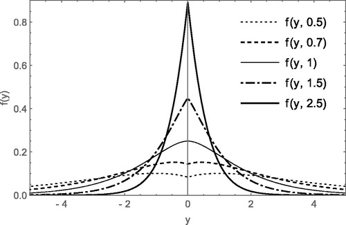
A distribution with p.d.f (2)(2) $$f\left(y;\theta \right)=\frac{{\theta }^2}{2\left(1+\theta \right)}\left(1+\left|y\right|\right)e^{-\theta \left|y\right|},$$(2) hereafter we denoted as DLD(θ), and a distribution with p.d.f (3)(3) $$f_1\left(y\right)=\{\begin{array}{ccc}\frac{1}{4}(1-y)e^y,& & y<0\\ \frac{1}{4}(1+y)e^{-y},& & y>0 .\end{array}$$(3) we named as standard double Lindley distribution (SDLD). Probability plots of the DLD(θ) are given in Figure 1 for particular values of θ. From Figure 1, we can observe that DLD exhibits unimodal and bimodal nature. On differentiating (2)(2) $$f\left(y;\theta \right)=\frac{{\theta }^2}{2\left(1+\theta \right)}\left(1+\left|y\right|\right)e^{-\theta \left|y\right|},$$(2) with respect to y, we obtain, (4) $$\frac{d}{dy}f(y;\theta )=f^{\prime }(y;\theta )=\{\begin{array}{cc}\frac{{\theta }^2}{2(1+\theta )}(\theta -\theta y-1){\mathrm{e}}^{\theta y},& y<0\\ \frac{{\theta }^2}{2(1+\theta )}(-\theta -\theta y+1){\mathrm{e}}^{-\theta y},& y\ge 0 .\end{array}$$(4)

Figure 1. The probability density function of the DLD for various values of θ.

Now, based on (4)(4) $$\frac{d}{dy}f(y;\theta )=f^{\prime }(y;\theta )=\{\begin{array}{cc}\frac{{\theta }^2}{2(1+\theta )}(\theta -\theta y-1){\mathrm{e}}^{\theta y},& y<0\\ \frac{{\theta }^2}{2(1+\theta )}(-\theta -\theta y+1){\mathrm{e}}^{-\theta y},& y\ge 0 .\end{array}$$(4) we have the following cases.

1. For $\theta <1,f^{\prime }(y;\theta )=0$ implies that $y_0=\frac{1-\theta }{\theta }$ and $\frac{\theta -1}{\theta }$ as the critical points at which $f(y;\theta )$ is maximum, which shows that the DLD is bimodal in this case.

2. For $\theta \ge 1,f^{\prime }(y;\theta )>0$ when $y<0$, so that $f(y;\theta )$ is increasing in y and $f^{\prime }(y;\theta )\le 0$ when $y\ge 0$, so that $f(y;\theta )$ is decreasing in y, which shows that the distribution is unimodal in this case and the mode is equal to zero.

Therefore, in the light of (4)(4) $$\frac{d}{dy}f(y;\theta )=f^{\prime }(y;\theta )=\{\begin{array}{cc}\frac{{\theta }^2}{2(1+\theta )}(\theta -\theta y-1){\mathrm{e}}^{\theta y},& y<0\\ \frac{{\theta }^2}{2(1+\theta )}(-\theta -\theta y+1){\mathrm{e}}^{-\theta y},& y\ge 0 .\end{array}$$(4) , the mode of the DLD is given by, (5) $$\mathit{\text{Mode}}=\{\begin{array}{ccc}\frac{1-\theta }{\theta }\hspace{0.5em}and\hspace{0.5em}\frac{\theta -1}{\theta },& & if\hspace{0.5em}\theta <1\\ 0,& & \mathit{\text{otherwise}} .\end{array}$$(5)

From (5)(5) $$\mathit{\text{Mode}}=\{\begin{array}{ccc}\frac{1-\theta }{\theta }\hspace{0.5em}and\hspace{0.5em}\frac{\theta -1}{\theta },& & if\hspace{0.5em}\theta <1\\ 0,& & \mathit{\text{otherwise}} .\end{array}$$(5) , we can say that when $\theta <1$, the distribution is bimodal and when $\theta \ge 1$, the distribution is unimodal.

Next, we obtain the cumulative distribution function (c.d.f) of the DLD(θ) as follows.

For $y<0$, the c.d.f of the DLD is, $$\begin{array}{c}F(y;\theta )={\int }_{-\infty }^y\frac{{\theta }^2}{2\left(1+\theta \right)}\left(1+\left|y\right|\right)e^{-\theta \left|y\right|}dy\\ =\frac{{\theta }^2}{2\left(1+\theta \right)}{\int }_{-\infty }^y(1-y)e^{\theta y}dy\\ =\frac{(\theta -\theta y+1)e^{\theta y}}{2(1+\theta )}\end{array}$$ and for $y\ge 0$, the c.d.f of the DLD is, $$\begin{array}{c}F(y;\theta )={\int }_{-\infty }^y\frac{{\theta }^2}{2\left(1+\theta \right)}\left(1+\left|y\right|\right)e^{-\theta \left|y\right|}dy\\ =\frac{{\theta }^2}{2\left(1+\theta \right)}\left({\int }_{-\infty }^0(1-y)e^{\theta y}dy+{\int }_0^y(1+y)e^{-\theta y}dy\right)\\ =1-\frac{(1+\theta +\theta y)}{2(1+\theta )}{e}^{-\theta y}.\end{array}$$ Thus, the c.d.f of the DLD with p.d.f (2)(2) $$f\left(y;\theta \right)=\frac{{\theta }^2}{2\left(1+\theta \right)}\left(1+\left|y\right|\right)e^{-\theta \left|y\right|},$$(2) is, (6) $$F\left(y;\theta \right)=\{\begin{array}{ccc}\frac{\left(\theta -\theta y+1\right)e^{\theta y}}{2\left(1+\theta \right)},& & y<0\\ 1-\frac{\left(1+\theta +\theta y\right)e^{-\theta y}}{2\left(1+\theta \right)},& & y\ge 0.\end{array}$$(6) When θ = 1 in (6)(6) $$F\left(y;\theta \right)=\{\begin{array}{ccc}\frac{\left(\theta -\theta y+1\right)e^{\theta y}}{2\left(1+\theta \right)},& & y<0\\ 1-\frac{\left(1+\theta +\theta y\right)e^{-\theta y}}{2\left(1+\theta \right)},& & y\ge 0.\end{array}$$(6) , we get the c.d.f of the SDLD as, (7) $$F_1\left(y\right)=\{\begin{array}{ccc}\frac{\left(2-y\right)e^y}{4},& & y<0\\ 1-\frac{\left(2+y\right)e^{-y}}{4},& & y\ge 0.\end{array}$$(7)

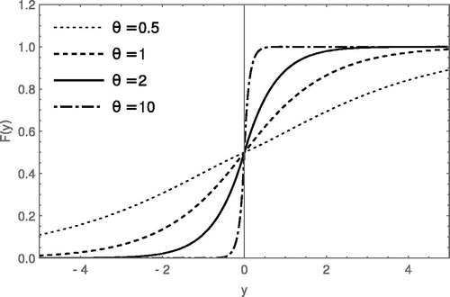
The non-decreasing and continuity nature shown by the c.d.f of the DLD can be observed from Figure 2 for various parameter values.

Figure 2. The cumulative distribution function of the DLD for different values of θ.

Next, we prove the following theorem, which gives how the DLD(θ) and Lindley(θ) are related.

Theorem 1.

If $Y\sim$ DLD (θ), then $Z=\left|Y\right|\sim$ Lindley (θ).

Proof.

For any $z>0$, the c.d.f of Z is, $$\begin{array}{c}P(Z\le z)=P(\left|Y\right|\le z)=P(-z\le Y\le z)\\ =F\left(z\right)-F(-z-0)\\ =1-\frac{(1+\theta +\theta z){\mathrm{e}}^{-\theta z}}{1+\theta },\end{array}$$ which is the c.d.f of the Lindley distribution with parameter θ. □

3. Moments and Generating Functions

In this section, we derive expressions for r^th raw moment, moment generating function and cumulant generating function of the DLD and discuss related properties of the distribution. In the case of DLD, we derive the general expression for the r^th moment as given below.

By definition, for $r\ge 1$, the r^th raw moment ${\mu }_r^{\prime }$ of the DLD is obtained as, (8) $$\begin{array}{c}{\mu }_r^{\prime }=E\left(Y^r\right)=\frac{{\theta }^2}{2\left(1+\theta \right)}{\int }_{-\infty }^{\infty }{y}^r\left(1+\left|y\right|\right)e^{-\theta \left|y\right|}dy\\ =\frac{{\theta }^2}{2\left(1+\theta \right)}\left({\int }_{-\infty }^0{y}^r\left(1-y\right)e^{\theta y}dy+{\int }_0^{\infty }{y}^r\left(1+y\right)e^{-\theta y}dy\right)\\ =\frac{{\theta }^2}{2\left(1+\theta \right)}\left(\frac{{(-1)}^r\Gamma (r+1)}{{\theta }^{r+1}}-\frac{{(-1)}^{r+1}\Gamma (r+2)}{{\theta }^{r+2}}+\frac{\Gamma (r+1)}{{\theta }^{r+1}}+\frac{\Gamma (r+2)}{{\theta }^{r+2}}\right)\\ =\{\begin{array}{ccc}\frac{r!\left(\theta +r+1\right)}{{\theta }^r\left(1+\theta \right)},& & \text{if}\hspace{0.5em}\mathrm{r}\hspace{0.5em}\text{is}\hspace{0.5em}\text{even}\\ 0,& & \text{if}\hspace{0.5em}\mathrm{r}\hspace{0.5em}\text{is}\hspace{0.5em}\text{odd} .\end{array}\end{array}$$(8) In particular, the $2^{nd},3^{rd}$, and $4^{th}$ central moments of the DLD take the form, $$\begin{array}{c}{\mu }_2=\mathit{\text{Variance}}=\frac{2!(\theta +3)}{{\theta }^2(\theta +1)},\\ {\mu }_3=0\end{array}$$ and $${\mu }_4=\frac{4!(\theta +5)}{{\theta }^4(\theta +1)}.$$

Thus, the coefficient of skewness ${\beta }_1$ and the coefficient of kurtosis ${\beta }_2$ of the DLD are, respectively, $${\beta }_1=\frac{{\mu }_3^2}{{\mu }_2^3}=0$$ and $${\beta }_2=\frac{{\mu }_4}{{\mu }_2^2}=\frac{3!(\theta +5)(1+\theta )}{{(\theta +3)}^2}.$$

Clearly, $\frac{d}{d\theta }{\beta }_2(\theta )>0$ for all $\theta >0$, the value of ${\beta }_2$ is minimum at θ = 0. Thus, ${\beta }_1=0$ and ${\beta }_2>3$ for all θ, which indicated that the DLD is always symmetric and leptokurtic.

Consequently, we have the following remark.

Remark 1.

For $r\ge 1$, the r^th raw moment of the standard DLD is, $${\mu }_r^{\prime }=\{\begin{array}{ccc}\frac{r!\left(r+2\right)}{2},& & \text{if}\hspace{0.5em}\mathrm{r}\hspace{0.5em}\text{is}\hspace{0.5em}\text{even}\\ 0,& & \text{if}\hspace{0.5em}\mathrm{r}\hspace{0.5em}\text{is}\hspace{0.5em}\text{odd}.\end{array}$$

For $r\ge 1$, the r^th absolute moment of the DLD is obtained as, (9) $$\begin{array}{c}{\delta }_r=E\left({\left|Y\right|}^r\right)=\frac{{\theta }^2}{2\left(1+\theta \right)}{\int }_{-\infty }^{\infty }{\left|y\right|}^r\left(1+\left|y\right|\right)e^{-\theta \left|y\right|}dy\\ =\frac{{\theta }^2}{2\left(1+\theta \right)}\left({\int }_{-\infty }^0{(-y)}^r\left(1-y\right)e^{\theta y}dy+{\int }_0^{\infty }{y}^r\left(1+y\right)e^{-\theta y}dy\right)\end{array}$$(9) (10) $$\begin{array}{c}=\frac{{\theta }^2}{2\left(1+\theta \right)}\left(\frac{\Gamma (r+1)}{{\theta }^{r+1}}+\frac{\Gamma (r+2)}{{\theta }^{r+2}}+\frac{\Gamma (r+1)}{{\theta }^{r+1}}+\frac{\Gamma (r+2)}{{\theta }^{r+2}}\right)\\ =\frac{r!\left(\theta +r+1\right)}{{\theta }^r\left(1+\theta \right)}.\end{array}$$(10)

It is to be noted that the mean deviation about mean (first absolute moment) of the DLD(θ) can be obtained when r = 1 in (10)(10) $$\begin{array}{c}=\frac{{\theta }^2}{2\left(1+\theta \right)}\left(\frac{\Gamma (r+1)}{{\theta }^{r+1}}+\frac{\Gamma (r+2)}{{\theta }^{r+2}}+\frac{\Gamma (r+1)}{{\theta }^{r+1}}+\frac{\Gamma (r+2)}{{\theta }^{r+2}}\right)\\ =\frac{r!\left(\theta +r+1\right)}{{\theta }^r\left(1+\theta \right)}.\end{array}$$(10) and is given by, $${\delta }_1=\frac{\theta +2}{\theta (\theta +1)}.$$

Now, we derive the moment generating function(m.g.f) $M_Y(t)$ of the DLD(θ) as follows. For any $t\in (-\theta ,\theta )$, by definition, the moment generating function (m.g.f) of the DLD with p.d.f (2)(2) $$f\left(y;\theta \right)=\frac{{\theta }^2}{2\left(1+\theta \right)}\left(1+\left|y\right|\right)e^{-\theta \left|y\right|},$$(2) is given by, (11) $$\begin{array}{c}{M}_Y\left(t\right)=E\left(e^{tY}\right)={\int }_{-\infty }^{\infty }{e}^{ty}\frac{{\theta }^2}{2(1+\theta )}(1+\left|y\right|)e^{-\theta \left|y\right|}dy\\ =\frac{{\theta }^2}{2(1+\theta )}\left\{{\int }_{-\infty }^0{e}^{(t+\theta )y}(1-y)dy+{\int }_0^{\infty }{e}^{(t-\theta )y}(1+y)dy\right\}\\ =\frac{{\theta }^2}{2(1+\theta )}\left\{\frac{1}{\theta +t}+\frac{1}{{(\theta +t)}^2}+\frac{1}{\theta -t}+\frac{1}{{(\theta -t)}^2}\right\}\\ =\frac{{\theta }^2({\theta }^3+{\theta }^2-\theta t^2+t^2)}{(1+\theta ){({\theta }^2-t^2)}^2}.\end{array}$$(11)

Clearly, when θ = 1, from (11)(11) $$\begin{array}{c}{M}_Y\left(t\right)=E\left(e^{tY}\right)={\int }_{-\infty }^{\infty }{e}^{ty}\frac{{\theta }^2}{2(1+\theta )}(1+\left|y\right|)e^{-\theta \left|y\right|}dy\\ =\frac{{\theta }^2}{2(1+\theta )}\left\{{\int }_{-\infty }^0{e}^{(t+\theta )y}(1-y)dy+{\int }_0^{\infty }{e}^{(t-\theta )y}(1+y)dy\right\}\\ =\frac{{\theta }^2}{2(1+\theta )}\left\{\frac{1}{\theta +t}+\frac{1}{{(\theta +t)}^2}+\frac{1}{\theta -t}+\frac{1}{{(\theta -t)}^2}\right\}\\ =\frac{{\theta }^2({\theta }^3+{\theta }^2-\theta t^2+t^2)}{(1+\theta ){({\theta }^2-t^2)}^2}.\end{array}$$(11) we have the m.g.f of the SDLD as, $$M_Y\left(t\right)=\frac{1}{{(1-t^2)}^2},for-1<t<1.$$

For any $t\in R$ and $i=\sqrt{-1}$, we can readily obtain the characteristic function(c.f) ${\varphi }_Y(t)$, of the DLD$(\theta )$, by replacing t by it in (11)(11) $$\begin{array}{c}{M}_Y\left(t\right)=E\left(e^{tY}\right)={\int }_{-\infty }^{\infty }{e}^{ty}\frac{{\theta }^2}{2(1+\theta )}(1+\left|y\right|)e^{-\theta \left|y\right|}dy\\ =\frac{{\theta }^2}{2(1+\theta )}\left\{{\int }_{-\infty }^0{e}^{(t+\theta )y}(1-y)dy+{\int }_0^{\infty }{e}^{(t-\theta )y}(1+y)dy\right\}\\ =\frac{{\theta }^2}{2(1+\theta )}\left\{\frac{1}{\theta +t}+\frac{1}{{(\theta +t)}^2}+\frac{1}{\theta -t}+\frac{1}{{(\theta -t)}^2}\right\}\\ =\frac{{\theta }^2({\theta }^3+{\theta }^2-\theta t^2+t^2)}{(1+\theta ){({\theta }^2-t^2)}^2}.\end{array}$$(11) and it is given by, (12) $${\varphi }_Y\left(t\right)=\frac{{\theta }^2\left({\theta }^3+{\theta }^2+\theta t^2-t^2\right)}{\left(1+\theta \right){\left({\theta }^2+t^2\right)}^2}.$$(12)

Remark 2.

If θ = 1 in (12)(12) $${\varphi }_Y\left(t\right)=\frac{{\theta }^2\left({\theta }^3+{\theta }^2+\theta t^2-t^2\right)}{\left(1+\theta \right){\left({\theta }^2+t^2\right)}^2}.$$(12) we get the c.f of SDLD as, (13) $${\psi }_Y\left(t\right)=\frac{1}{{\left(1+t^2\right)}^2}.$$(13) which shows that ${\psi }_Y(t)=R_{Z_1}(t).R_{Z_2}(t)$, where Z₁, Z₂ are independent standard Laplace random variables, so that the SDLD random variate can be viewed as the sum of two independent standard Laplace random variables.

The cumulant generating function of DLD is, (14) $$\begin{array}{c}{K}_Y\left(t\right)=\sum _{n=1}^{\infty }{K}_n\frac{t^n}{n!}\\ \end{array}$$(14) $$=\hspace{0.17em}\text{log}\left[M_Y\right(t\left)\right]=\hspace{0.17em}\text{log}\hspace{0.17em}\left[\frac{{\theta }^2\left({\theta }^3+{\theta }^2-\theta t^2+t^2\right)}{(1+\theta ){(\theta +t)}^2{(\theta -t)}^2}\right]\begin{array}{l}=\hspace{0.17em}\text{log}\hspace{0.17em}\left[\frac{\left(1+\frac{{\theta }^2-\theta t^2+t^2}{{\theta }^3}\right)}{\left(1+\frac{1}{\theta }\right){\left(1+\frac{t}{\theta }\right)}^2{\left(1-\frac{t}{\theta }\right)}^2}\right]\end{array}$$ (15) $$\begin{array}{c}=\hspace{0.17em}\text{log}\hspace{0.17em}\left(1+\frac{{\theta }^2-\theta t^2+t^2}{{\theta }^3}\right)-\hspace{0.17em}\text{log}\hspace{0.17em}\left(1+\frac{1}{\theta }\right)-2\hspace{0.17em}\text{log}\hspace{0.17em}\left(1+\frac{t}{\theta }\right)-2\hspace{0.17em}\text{log}\hspace{0.17em}\left(1-\frac{t}{\theta }\right).\end{array}$$(15)

Now, by expanding the logarithmic terms in (15)(15) $$\begin{array}{c}=\hspace{0.17em}\text{log}\hspace{0.17em}\left(1+\frac{{\theta }^2-\theta t^2+t^2}{{\theta }^3}\right)-\hspace{0.17em}\text{log}\hspace{0.17em}\left(1+\frac{1}{\theta }\right)-2\hspace{0.17em}\text{log}\hspace{0.17em}\left(1+\frac{t}{\theta }\right)-2\hspace{0.17em}\text{log}\hspace{0.17em}\left(1-\frac{t}{\theta }\right).\end{array}$$(15) , we obtain the following. (16) $$\begin{array}{c}{K}_Y\left(t\right)=\frac{(3+\theta )t^2}{{\theta }^2(1+\theta )}+\frac{(1+6\theta +{\theta }^2)t^4}{2{\theta }^4{(1+\theta )}^2}+\frac{(3+3\theta +9{\theta }^2+{\theta }^3)t^6}{3{\theta }^6{(1+\theta )}^3}+\dots \\ \hspace{1em}\hspace{1em}\hspace{1em}\hspace{1em}+\frac{\left(2n\right)!\left({(3+\theta )}^n-2n(2n-2)!{(1+\theta )}^{n-2}\right)}{n{\left({\theta }^2(1+\theta )\right)}^n}+\dots \end{array}$$(16)

On equating coefficients of $\frac{t^n}{n!}$ in the right hand side expression of (14)(14) $$\begin{array}{c}{K}_Y\left(t\right)=\sum _{n=1}^{\infty }{K}_n\frac{t^n}{n!}\\ \end{array}$$(14) and (16)(16) $$\begin{array}{c}{K}_Y\left(t\right)=\frac{(3+\theta )t^2}{{\theta }^2(1+\theta )}+\frac{(1+6\theta +{\theta }^2)t^4}{2{\theta }^4{(1+\theta )}^2}+\frac{(3+3\theta +9{\theta }^2+{\theta }^3)t^6}{3{\theta }^6{(1+\theta )}^3}+\dots \\ \hspace{1em}\hspace{1em}\hspace{1em}\hspace{1em}+\frac{\left(2n\right)!\left({(3+\theta )}^n-2n(2n-2)!{(1+\theta )}^{n-2}\right)}{n{\left({\theta }^2(1+\theta )\right)}^n}+\dots \end{array}$$(16) , we get the n^th cumulant, K_n of the DLD as follows. (17) $$K_n=\{\begin{array}{cc}\frac{2!(3+\theta )}{{\theta }^2(1+\theta )},& n=2\\ & \\ \frac{n!\left[\left\{2{\theta }^{-n}-{\left(\frac{\sqrt{(\theta -1)}}{\sqrt{{\theta }^2(1+\theta )}}\right)}^n\right\}\left({(-1)}^n+1\right)\right]}{n},& n\ge 4.\end{array}$$(17)

From (17)(17) $$K_n=\{\begin{array}{cc}\frac{2!(3+\theta )}{{\theta }^2(1+\theta )},& n=2\\ & \\ \frac{n!\left[\left\{2{\theta }^{-n}-{\left(\frac{\sqrt{(\theta -1)}}{\sqrt{{\theta }^2(1+\theta )}}\right)}^n\right\}\left({(-1)}^n+1\right)\right]}{n},& n\ge 4.\end{array}$$(17) , it can be noted that all the odd cumulants of DLD are zero. In particular, the first few even order cumulants of the DLD are, $$\begin{array}{c}{K}_4=\frac{4!(1+6\theta +{\theta }^2)}{2{\theta }^4{(1+\theta )}^2},\\ K_6=\frac{6!(3+3\theta +9{\theta }^2+{\theta }^3)}{3{\theta }^6{(1+\theta )}^3},\\ K_8=\frac{8!(1+12\theta +6{\theta }^2+12{\theta }^3+{\theta }^4)}{4{\theta }^8{(1+\theta )}^4}.\end{array}$$

4. Reliability Measures

It is essential to derive expressions for the reliability measures, like survival function, hazard function, and mean residual life function for DLD since it can be used to study the reliability of a system involving one unit.

The survival function S(y) of the DLD(θ) is given by, (18) $$\begin{array}{c}S\left(y\right)=1-F(y;\theta )\\ =\{\begin{array}{ccc}1-\frac{\left(\theta -\theta y+1\right)e^{\theta y}}{2\left(1+\theta \right)},& & y<0\\ \frac{\left(1+\theta +\theta y\right)e^{-\theta y}}{2\left(1+\theta \right)},& & y\ge 0\end{array}\end{array}$$(18) and the failure rate function (hazard rate function) of the DLD(θ) is given by, (19) $$h\left(y\right)=\{\begin{array}{ccc}\frac{{\theta }^2\left(1-y\right)e^{\theta y}}{2\left(1+\theta \right)-\left(\theta -\theta y+1\right)e^{\theta y}},& & y<0\\ \frac{{\theta }^2\left(1+y\right)}{1+\theta +\theta y},& & y\ge 0 .\end{array}$$(19)

The proof follows directly from the definition of hazard rate function and is, hence, omitted.

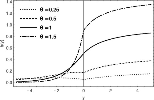
It is important to analyze whether the failure rate function is increasing or decreasing, because this phenomenon describes where the probability of an event in a fixed time interval in the future increases or decreases over time. The failure rate function of the DLD is graphically represented in Figure 3. From Figure 3, we can observe that the failure rate function of the DLD shows both increasing and decreasing failure rates. The following theorem establishes the nature of the failure rate function of the DLD in a more precise manner.

Figure 3. The hazard rate function of the DLD for various parameter values.

Theorem 2.

If Y follows DLD with failure rate function as given in (19)(19) $$h\left(y\right)=\{\begin{array}{ccc}\frac{{\theta }^2\left(1-y\right)e^{\theta y}}{2\left(1+\theta \right)-\left(\theta -\theta y+1\right)e^{\theta y}},& & y<0\\ \frac{{\theta }^2\left(1+y\right)}{1+\theta +\theta y},& & y\ge 0 .\end{array}$$(19) , then Y has decreasing failure rate (DFR) for any $\theta <1$ such that $1-\frac{1}{\theta }\le y<0$ and non-decreasing failure rate (IFR) elsewhere.

Proof.

On differentiating (19)(19) $$h\left(y\right)=\{\begin{array}{ccc}\frac{{\theta }^2\left(1-y\right)e^{\theta y}}{2\left(1+\theta \right)-\left(\theta -\theta y+1\right)e^{\theta y}},& & y<0\\ \frac{{\theta }^2\left(1+y\right)}{1+\theta +\theta y},& & y\ge 0 .\end{array}$$(19) with respect to y, we have, (20) $$\frac{d}{dy}h\left(y\right)=\{\begin{array}{ccc}\frac{{\mathrm{e}}^{\theta y}{\theta }^2\left[e^{\theta y}-2(1+\theta )(1-\theta +\theta y)\right]}{{\left[2\left(1+\theta \right)-e^{\theta y}\left(1+\theta -\theta y\right)\right]}^2},& & y<0\\ \frac{{\theta }^2}{{(1+\theta +\theta y)}^2},& & y\ge 0.\end{array}$$(20)

From (20)(20) $$\frac{d}{dy}h\left(y\right)=\{\begin{array}{ccc}\frac{{\mathrm{e}}^{\theta y}{\theta }^2\left[e^{\theta y}-2(1+\theta )(1-\theta +\theta y)\right]}{{\left[2\left(1+\theta \right)-e^{\theta y}\left(1+\theta -\theta y\right)\right]}^2},& & y<0\\ \frac{{\theta }^2}{{(1+\theta +\theta y)}^2},& & y\ge 0.\end{array}$$(20) , it follows that when $\theta <1,\frac{d[h(y)]}{dy}<0$ for $1-\frac{1}{\theta }<y<0$ and $\frac{d[h(y)]}{dy}>0$, for all other values of y and θ. Therefore, for $\theta <1$ such that $1-\frac{1}{\theta }\le y<0$, the hazard rate function of DLD is DFR and when $\theta \ge 1$ and $y<1-\frac{1}{\theta }$ it is IFR. The hazard rate function is IFR for all values of θ when $y\ge 0$.□

Lariviere and Porteus (2001) has defined the generalized failure rate of a continuous random variable X with hazard rate function h(x) as $g(x)=xh(x)$. Thus, X has an increasing generalized failure rate (IGFR) if g(x) is non-decreasing and decreasing generalized failure rate (DGFR) if g(x) is non-increasing. Generalized failure rate distributions have various applications in the areas of inventory management, pricing and supply chain problems etc. The GFR nature of DLD is stated in the following theorem.

Theorem 3.

If Y follows DLD with failure rate function as given in (19)(19) $$h\left(y\right)=\{\begin{array}{ccc}\frac{{\theta }^2\left(1-y\right)e^{\theta y}}{2\left(1+\theta \right)-\left(\theta -\theta y+1\right)e^{\theta y}},& & y<0\\ \frac{{\theta }^2\left(1+y\right)}{1+\theta +\theta y},& & y\ge 0 .\end{array}$$(19) , then Y has decreasing generalized failure rate (DGFR) for $y<\frac{(\theta -2)-\sqrt{({\theta }^2+4)}}{2\theta }$ and increasing generalized failure rate (IGFR) elsewhere.

Proof.

In the case of DLD, $$g\left(y\right)=y h\left(y\right)=\{\begin{array}{ccc}\frac{{\theta }^{2}y\left(1-y\right)e^{\theta y}}{2\left(1+\theta \right)-\left(\theta -\theta y+1\right)e^{\theta y}},& & y<0\\ \frac{{\theta }^{2}y(1+y)}{(1+\theta +\theta y)},& & y\ge 0\end{array}$$ and (21) $$\frac{d}{dy}g\left(y\right)=g^{\prime }\left(y\right)=\{\begin{array}{cc}\frac{e^{\theta y}{\theta }^2\left[-e^{\theta y}(1-2y+{(y-1)}^2\theta )-2(1+\theta )(-1+2y+(y-1)\theta y)\right]}{{\left[2\left(1+\theta \right)-e^{\theta y}\left(\theta -\theta y+1\right)\right]}^2},& y<0\\ \frac{{\theta }^2\left[1+2y+{(y+1)}^2\theta \right]}{{(1+\theta +\theta y)}^2},& y\ge 0.\end{array}$$(21)

From (21)(21) $$\frac{d}{dy}g\left(y\right)=g^{\prime }\left(y\right)=\{\begin{array}{cc}\frac{e^{\theta y}{\theta }^2\left[-e^{\theta y}(1-2y+{(y-1)}^2\theta )-2(1+\theta )(-1+2y+(y-1)\theta y)\right]}{{\left[2\left(1+\theta \right)-e^{\theta y}\left(\theta -\theta y+1\right)\right]}^2},& y<0\\ \frac{{\theta }^2\left[1+2y+{(y+1)}^2\theta \right]}{{(1+\theta +\theta y)}^2},& y\ge 0.\end{array}$$(21) , it follows that when $y<\frac{(\theta -2)-\sqrt{({\theta }^2+4)}}{2\theta },g^{\prime }(y)<0$ and for $y\ge \frac{(\theta -2)-\sqrt{({\theta }^2+4)}}{2\theta },g^{\prime }(y)>0$. Therefore, for $y<\frac{(\theta -2)-\sqrt{({\theta }^2+4)}}{2\theta }$, the hazard rate function h(y) of the DLD is DGFR and for all other values of y, it is IGFR. □

In reliability studies, life expectancy or mean residual life is an important characteristic of the model. In life tesing situations, it is exciting to know about the expected additional lifetime of a component given that it has survived until a particular time. Based on the survival function given in (18)(18) $$\begin{array}{c}S\left(y\right)=1-F(y;\theta )\\ =\{\begin{array}{ccc}1-\frac{\left(\theta -\theta y+1\right)e^{\theta y}}{2\left(1+\theta \right)},& & y<0\\ \frac{\left(1+\theta +\theta y\right)e^{-\theta y}}{2\left(1+\theta \right)},& & y\ge 0\end{array}\end{array}$$(18) , one can compute the mean residual life function of the DLD as follows.

For $y<0$, the MRLF of the DLD is given by, $$\begin{array}{c}m\left(y\right)=\frac{1}{1-\frac{(\theta -\theta y+1)e^{\theta y}}{2(1+\theta )}}{\int }_y^0\left(1-\frac{(\theta -\theta t+1)e^{\theta t}}{2(1+\theta )}\right)dt\\ =\frac{-2y\theta \left(1+\theta \right)+e^{\theta y}\left(2+\theta -\theta y\right)-(2+\theta )}{\theta \left(2\left(1+\theta \right)+e^{\theta y}\left(-1+\left(y-1\right)\theta \right)\right)}\end{array}$$ and for $y>0$, the mean residual life function (MRLF) of the DLD is given by, $$\begin{array}{c}m\left(y\right)=E\left[Y-y|Y>y\right]=\frac{1}{1-F\left(y\right)}\underset{y}{\overset{\infty }{\int }}\left(1-F\left(t\right)\right)dt\\ =\frac{2(1+\theta )}{(1+\theta +\theta y)e^{-\theta y}}{\int }_y^{\infty }\frac{(1+\theta +\theta t)e^{-\theta t}}{2(1+\theta )}dt\\ =\frac{2+\theta +\theta y}{\theta \left(1+\theta +\theta y\right)}.\end{array}$$

Thus, the MRLF of the DLD is, (22) $$m\left(y\right) =\{\begin{array}{ccc}\frac{-2y\theta \left(1+\theta \right)+e^{\theta y}\left(2+\theta -\theta y\right)-(2+\theta )}{\theta \left(2\left(1+\theta \right)+e^{\theta y}\left(-1+\left(y-1\right)\theta \right)\right)},& & y<0\\ \frac{2+\theta +\theta y}{\theta \left(1+\theta +\theta y\right)},& & y>0.\end{array}$$(22)

5. Order Statistics

In this section, we derive the distribution of order statistics and the q^th moment of the k^th order statistics of the DLD.

Suppose $Y_1, Y_2, \dots , Y_n$ is a random sample from (2)(2) $$f\left(y;\theta \right)=\frac{{\theta }^2}{2\left(1+\theta \right)}\left(1+\left|y\right|\right)e^{-\theta \left|y\right|},$$(2) . Let $Y_{1:n}<Y_{2:n}<\dots <Y_{n:n}$ denote the corresponding order statistics. For $k\ge 1$, the p.d.f and c.d.f of the k^th order statistic $Y_{k:n}$ of the DLD are given by, (23) $$f_{Y_{k:n}}\left(y\right)=\{\begin{array}{ccc}\frac{n!{\theta }^2(1-y)e^{\theta y}}{(k-1)!(n-k)!2(1+\theta )}\sum _{r=0}^{n-k}\left(\begin{array}{c}n-k\\ r\end{array}\right){(-1)}^r{\left[\frac{(1-\theta (y-1\left)\right)e^{\theta y}}{2(1+\theta )}\right]}^{k+r-1},& & y<0\\ \frac{n!{\theta }^2(1+y)e^{-\theta y}}{(k-1)!(n-k)!2(1+\theta )}\sum _{r=0}^{n-k}\left(\begin{array}{c}n-k\\ r\end{array}\right){(-1)}^r{\left[1-\frac{(1+\theta (y+1\left)\right)e^{-\theta y}}{2(1+\theta )}\right]}^{k+r-1},& & y\ge 0\end{array}$$(23) and (24) $$F_{Y_{k:n}}\left(y\right)=\{\begin{array}{ccc}\sum _{j=k}^n\sum _{r=0}^{n-j}\left(\begin{array}{c}n\\ j\end{array}\right)\left(\begin{array}{c}n-j\\ r\end{array}\right){(-1)}^r{\left[\frac{(1-\theta (y-1\left)\right)e^{\theta y}}{2(1+\theta )}\right]}^{j+r},& & y<0\\ \sum _{j=k}^n\sum _{r=0}^{n-j}\left(\begin{array}{c}n\\ j\end{array}\right)\left(\begin{array}{c}n-j\\ r\end{array}\right){(-1)}^r{\left[1-\frac{(1+\theta (y+1\left)\right)e^{-\theta y}}{2(1+\theta )}\right]}^{j+r},& & y\ge 0.\end{array}$$(24) respectively. Now, by using (23)(23) $$f_{Y_{k:n}}\left(y\right)=\{\begin{array}{ccc}\frac{n!{\theta }^2(1-y)e^{\theta y}}{(k-1)!(n-k)!2(1+\theta )}\sum _{r=0}^{n-k}\left(\begin{array}{c}n-k\\ r\end{array}\right){(-1)}^r{\left[\frac{(1-\theta (y-1\left)\right)e^{\theta y}}{2(1+\theta )}\right]}^{k+r-1},& & y<0\\ \frac{n!{\theta }^2(1+y)e^{-\theta y}}{(k-1)!(n-k)!2(1+\theta )}\sum _{r=0}^{n-k}\left(\begin{array}{c}n-k\\ r\end{array}\right){(-1)}^r{\left[1-\frac{(1+\theta (y+1\left)\right)e^{-\theta y}}{2(1+\theta )}\right]}^{k+r-1},& & y\ge 0\end{array}$$(23) , we obtain the following result.

Result 1.

The q^th moment of the k^th order statistic,$Y_{k:n}$ of the DLD is given by, (25) $$\begin{array}{c}E\left(Y_{k:n}^q\right)=\frac{n!{\theta }^2}{(k-1)!(n-k)!2(1+\theta )}\{\sum _{r=0}^{n-k} \sum _{j=0}^{k+r-1}\sum _{i=0}^j\left(\begin{array}{c}n-k\\ r\end{array}\right)\left(\begin{array}{c}k+r-1\\ j\end{array}\right)\left(\begin{array}{c}j\\ i\end{array}\right)\\ \times \frac{{(-1)}^{r+q}{\theta }^j(q+i)!}{2(1+\theta ){\left[\theta (k+r)\right]}^{q+i+2}}\left[\theta (k+r)+q+i+1\right]\\ +\sum _{r=0}^{n-k} \sum _{j=0}^{k+r-1}\sum _{i=0}^j\sum _{m=0}^i\left(\begin{array}{c}n-k\\ r\end{array}\right)\left(\begin{array}{c}k+r-1\\ j\end{array}\right)\left(\begin{array}{c}j\\ i\end{array}\right)\left(\begin{array}{c}i\\ m\end{array}\right)\\ \times \frac{{(-1)}^{r+j}{\theta }^i(q+m)!}{{\left[2(1+\theta )\right]}^j{\left[\theta (j+1)\right]}^{q+m+2}}\left[\theta (j+1)+q+m+1\right]\}.\end{array}$$(25)

Proof.

$$\begin{array}{c}E\left(Y_{k:n}^q\right)={\int }_{-\infty }^{\infty }{y}^q{f}_{k:n}\left(y\right)dy\\ =\frac{n!{\theta }^2}{(k-1)!(n-k)!2(1+\theta )}\{\sum _{r=0}^{n-k}\frac{\left(\begin{array}{c}n-k\\ r\end{array}\right){(-1)}^r}{{\left[2(1+\theta )\right]}^{k-1+r}}\\ \times {\int }_{-\infty }^0\left[y^q(1-y)e^{\theta (k+r)y}{\left[1-\theta (y-1)\right]}^{k-1+r}\right]dy\\ +\sum _{r=0}^{n-k}\left(\begin{array}{c}n-k\\ r\end{array}\right){(-1)}^r{\int }_0^{\infty }\left[y^q(1+y)e^{-\theta y}{\left[1-\frac{(1+\theta (1+y\left)\right)e^{-\theta y}}{2(1+\theta )}\right]}^{k+r-1}\right]dy\}\\ =\frac{n!{\theta }^2}{(k-1)!(n-k)!2(1+\theta )}\{\sum _{r=0}^{n-k}\sum _{j=0}^{k-1+r}\sum _{i=0}^j\left(\begin{array}{c}n-k\\ r\end{array}\right)\left(\begin{array}{c}k-1+r\\ j\end{array}\right)\left(\begin{array}{c}j\\ i\end{array}\right)\\ \times \frac{{(-1)}^{r+i}{\theta }^j}{{\left[2(1+\theta )\right]}^{k-1+r}}{\int }_{-\infty }^0\left[y^{q+i}(1-y)e^{\theta (k+r)y}\right]dy\\ +\sum _{r=0}^{n-k}\sum _{j=0}^{k-1+r}\sum _{i=0}^j\left(\begin{array}{c}n-k\\ r\end{array}\right)\left(\begin{array}{c}k-1+r\\ j\end{array}\right)\left(\begin{array}{c}j\\ i\end{array}\right)\frac{{(-1)}^{l+j}{\theta }^i}{{\left[2(1+\theta )\right]}^j}\\ \times {\int }_0^{\infty }\left[y^q(1+y)e^{-\theta (j+1)y}\sum _{m=0}^i\left(\begin{array}{c}i\\ m\end{array}\right)y^i\right]dy\},\end{array}$$ by binomial expansion, then we get (25)(25) $$\begin{array}{c}E\left(Y_{k:n}^q\right)=\frac{n!{\theta }^2}{(k-1)!(n-k)!2(1+\theta )}\{\sum _{r=0}^{n-k} \sum _{j=0}^{k+r-1}\sum _{i=0}^j\left(\begin{array}{c}n-k\\ r\end{array}\right)\left(\begin{array}{c}k+r-1\\ j\end{array}\right)\left(\begin{array}{c}j\\ i\end{array}\right)\\ \times \frac{{(-1)}^{r+q}{\theta }^j(q+i)!}{2(1+\theta ){\left[\theta (k+r)\right]}^{q+i+2}}\left[\theta (k+r)+q+i+1\right]\\ +\sum _{r=0}^{n-k} \sum _{j=0}^{k+r-1}\sum _{i=0}^j\sum _{m=0}^i\left(\begin{array}{c}n-k\\ r\end{array}\right)\left(\begin{array}{c}k+r-1\\ j\end{array}\right)\left(\begin{array}{c}j\\ i\end{array}\right)\left(\begin{array}{c}i\\ m\end{array}\right)\\ \times \frac{{(-1)}^{r+j}{\theta }^i(q+m)!}{{\left[2(1+\theta )\right]}^j{\left[\theta (j+1)\right]}^{q+m+2}}\left[\theta (j+1)+q+m+1\right]\}.\end{array}$$(25) , by evaluating the integrals. □

The above results on the distribution of order statistics and its q^th moment will be much useful for inference problems as well.

6. Entropy

In this section, we derive Rényi entropy measure of the DLD. An entropy of a random variable X is a measure of variation of the uncertainty.

By definition, Rényi entropy of a distribution with p.d.f $f(.)$ is given by, (26) $$I_R(\gamma )=\frac{1}{1-\gamma }\text{log}\hspace{0.17em}\left\{\int f^{\gamma }\left(x\right)dx\right\},$$(26) where $\gamma >0$ and $\gamma \ne 1$. Thus, the Rényi entropy of DLD with p.d.f (2)(2) $$f\left(y;\theta \right)=\frac{{\theta }^2}{2\left(1+\theta \right)}\left(1+\left|y\right|\right)e^{-\theta \left|y\right|},$$(2) is given by, $$I_R(\gamma )=\frac{1}{1-\gamma }\text{log}\hspace{0.17em}\left\{\int f^{\gamma }\left(y\right)dx\right\},$$ in which, $$\begin{array}{c}\int f^{\gamma }\left(y\right)dy={\int }_{-\infty }^{\infty }{\left[\frac{{\theta }^2}{2\left(1+\theta \right)}\left(1+\left|y\right|\right)e^{-\theta \left|y\right|}\right]}^{\gamma }dy\\ =\frac{{\theta }^{2\gamma }}{2^{\gamma }{(1+\theta )}^{\gamma }}\left\{{\int }_{-\infty }^0{(1-y)}^{\gamma }{e}^{\theta \gamma y}dy+{\int }_0^{\infty }{(1+y)}^{\gamma }{e}^{-\theta \gamma y}dy\right\}.\end{array}$$

Now, using the series expansions, (27) $${(1+x)}^a=\sum _{j=0}^{\infty }{(a+1-j)}_j\frac{x^j}{j!}$$(27) and (28) $${(1-x)}^a=\sum _{j=0}^{\infty }{(a+1-j)}_j\frac{{(-1)}^j{x}^j}{j!}$$(28) for any $a\in R$ and ${(x)}_k=x(x+1)\dots (x+k-1)$ for $k\ge 1$ with ${(x)}_0=1$ (Pochhammer symbol). Then, we get, $$\begin{array}{c}\int f^{\gamma }\left(y\right)dy=\frac{{\theta }^{2\gamma }}{2^{\gamma }{(1+\theta )}^{\gamma }}\{{\int }_{-\infty }^0\sum _{j=0}^{\infty }{(\gamma +1-j)}_j\frac{{(-1)}^j{y}^j}{j!}{e}^{\theta \gamma y}dy\\ \hspace{1em}+{\int }_0^{\infty }\sum _{j=0}^{\infty }{(\gamma +1-j)}_j\frac{y^j}{j!}{e}^{-\theta \gamma y}dy\}\\ =\frac{{\theta }^{2\gamma }}{2^{\gamma -1}{(1+\theta )}^{\gamma }}\sum _{j=0}^{\infty }{(\gamma +1-j)}_j\frac{\Gamma (j+1)}{j!{(\theta \gamma )}^{j+1}}.\end{array}$$ Here, using the expression, ${(a-n)}_n={(-1)}^n{(1-a)}_n$, we can write, $$\int f^{\gamma }\left(y\right)dy={\frac{{\theta }^{2\gamma -1}}{2^{\gamma -1}\gamma {(1+\theta )}^{\gamma }}}_{\mathrm{}}{}_2{F}_1(-\gamma ,1; ;\frac{-1}{\theta \gamma }).$$ Then, the entropy of DLD is obtained as, (29) $$\begin{array}{c}{I}_R(\gamma )=\frac{1}{1-\gamma }[(2\gamma -1)\hspace{0.17em}\text{log}(\theta )-(\gamma -1)\hspace{0.17em}\text{log}\left(2\right)-\gamma \hspace{0.17em}\text{log}(1+\theta )-\hspace{0.17em}\text{log}(\gamma )\\ +\hspace{0.17em}\text{log}\hspace{0.17em}{(}_2{F}_1(-\gamma ,1; ;\frac{-1}{\theta \gamma }))],\end{array}$$(29) where (30) $${}_2{F}_1(a,b;c;\theta )=\sum _{j=0}^{\infty }\frac{{\left(a\right)}_j{\left(b\right)}_j}{{\left(c\right)}_j}\frac{{\theta }^j}{j!}$$(30) is the Gauss Hypergeometric Function.

7. Location Scale Extension

Here, we consider an extended form of the DLD by introducing the location parameter μ and scale parameter σ in the p.d.f of DLD and call it as” the extended double Lindley distribution (EDLD)”. We define the EDLD as follows.

Definition 2.

Let $Y\sim DLD(\theta )$ with p.d.f. (2)(2) $$f\left(y;\theta \right)=\frac{{\theta }^2}{2\left(1+\theta \right)}\left(1+\left|y\right|\right)e^{-\theta \left|y\right|},$$(2) . Then $Z=\mu +\sigma Y$ is said to have an extended double Lindley distribution (EDLD) with parameters $\theta , \mu$ and σ and its p.d.f is of the form, (31) $$f\left(z;\theta ,\mu ,\sigma \right)=\frac{{\theta }^2}{2\left(1+\theta \right)\sigma }\left(1+\left|\frac{z-\mu }{\sigma }\right|\right){\mathrm{e}}^{-\theta \left|\frac{z-\mu }{\sigma }\right|},$$(31) for $-\infty <z<\infty ,\theta >0,-\infty <\mu <\infty$ and $\sigma >0$.

We denote the distribution with p.d.f (31)(31) $$f\left(z;\theta ,\mu ,\sigma \right)=\frac{{\theta }^2}{2\left(1+\theta \right)\sigma }\left(1+\left|\frac{z-\mu }{\sigma }\right|\right){\mathrm{e}}^{-\theta \left|\frac{z-\mu }{\sigma }\right|},$$(31) as EDLD$(\theta , \mu , \sigma )$. Analogous to the findings in the case of DLD, here, we are given expressions for certain characteristics of EDLD, which we present through the following results. Their proofs are omitted, as they are the direct consequence of the corresponding expressions given in sections 2–6.

Result 2.

The cumulative distribution function of the EDLD is given by, (32) $$F\left(z;\theta ,\mu ,\sigma \right)=\{\begin{array}{lll}-\frac{{\mathrm{e}}^{\theta \left(\frac{z-\mu }{\sigma }\right)}\left(\theta z-\theta \mu -\sigma -\theta \sigma \right)}{2\left(1+\theta \right)\sigma },& & z<\mu \\ \frac{2\theta \sigma +2\sigma -\left(\theta \sigma +\theta z+\sigma -\theta \mu \right){\mathrm{e}}^{-\theta \left(\frac{z-\mu }{\sigma }\right)}}{2\left(1+\theta \right)\sigma },& & z\ge \mu .\end{array}$$(32)

When we put μ = 0 and σ = 1 in (32)(32) $$F\left(z;\theta ,\mu ,\sigma \right)=\{\begin{array}{lll}-\frac{{\mathrm{e}}^{\theta \left(\frac{z-\mu }{\sigma }\right)}\left(\theta z-\theta \mu -\sigma -\theta \sigma \right)}{2\left(1+\theta \right)\sigma },& & z<\mu \\ \frac{2\theta \sigma +2\sigma -\left(\theta \sigma +\theta z+\sigma -\theta \mu \right){\mathrm{e}}^{-\theta \left(\frac{z-\mu }{\sigma }\right)}}{2\left(1+\theta \right)\sigma },& & z\ge \mu .\end{array}$$(32) , it reduces to the c.d.f of the DLD as given in (6)(6) $$F\left(y;\theta \right)=\{\begin{array}{ccc}\frac{\left(\theta -\theta y+1\right)e^{\theta y}}{2\left(1+\theta \right)},& & y<0\\ 1-\frac{\left(1+\theta +\theta y\right)e^{-\theta y}}{2\left(1+\theta \right)},& & y\ge 0.\end{array}$$(6) .

Result 3.

For $r>0$, the r^th moment, ${\mu }_r^{\prime }$ about origin of EDLD is, (33) $$\begin{array}{c}{\mu }_r^{\prime }=\frac{{\mathrm{e}}^{-\frac{\theta \mu }{\sigma }}{\sigma }^{r-1}}{2(\theta +1){(-\theta )}^r}[\left(\theta (\mu +\sigma )\Gamma (r+1,-\frac{\theta \mu }{\sigma })+\sigma \Gamma (r+2,-\frac{\theta \mu }{\sigma }\right))\\ +{\mathrm{e}}^{\frac{2\theta \mu }{\sigma }}{(-1)}^r\left(\theta (\sigma -\mu ) \Gamma (r+1,\frac{\theta \mu }{\sigma })+\sigma \Gamma (r+2,\frac{\theta \mu }{\sigma }\right))].\end{array}$$(33)

Result 4.

For $r>0$, the central moments of the EDLD are given by, (34) $${\mu }_r=\frac{(\theta +r+1)\Gamma (r+1){\left(\frac{\sigma }{\theta }\right)}^r\left[{(-1)}^r+1\right]}{2(\theta +1)}.$$(34)

From (34)(34) $${\mu }_r=\frac{(\theta +r+1)\Gamma (r+1){\left(\frac{\sigma }{\theta }\right)}^r\left[{(-1)}^r+1\right]}{2(\theta +1)}.$$(34) , we can find that all the odd central moments of EDLD are zero. In particular, for the EDLD, we have, $$\begin{array}{c}{\mu }_1^{\prime }=\mathrm{\text{Mean}}=\mu ,\\ {\mu }_2=\mathrm{\text{Variance}}=\frac{2(\theta +3){\sigma }^2}{{\theta }^2(\theta +1)},\\ {\mu }_3=0\end{array}$$ and $${\mu }_4=\frac{24(\theta +5){\sigma }^4}{{\theta }^4(\theta +1)}.$$

Remark 3.

The coefficient of variation $(\gamma )$, coefficient of skewness $({\beta }_1)$ and the coefficient of kurtosis $({\beta }_2)$ of the EDLD are given below. $$\begin{array}{c}\gamma =\frac{\sigma }{\theta \mu }\sqrt{\frac{2(\theta +3)}{(\theta +1)}},\\ {\beta }_1=0\end{array}$$ and $${\beta }_2=\frac{3!(\theta +5)(\theta +1)}{{(\theta +3)}^2}.$$

Result 5.

For $r\ge 1$, the r^th absolute moment of the EDLD is given by, (35) $${\delta }_r=E\left({\left|Z\right|}^r\right)=\frac{r!{\sigma }^r\left(\theta +r+1\right)}{{\theta }^r\left(1+\theta \right)}.$$(35)

From (35)(35) $${\delta }_r=E\left({\left|Z\right|}^r\right)=\frac{r!{\sigma }^r\left(\theta +r+1\right)}{{\theta }^r\left(1+\theta \right)}.$$(35) , when r = 1, we can obtain the mean deviation about mean of the EDLD as, $${\delta }_1=\frac{\sigma (\theta +2)}{\theta (\theta +1)}.$$

Result 6.

The characteristic function of EDLD is given by, (36) $${\varphi }_Z\left(t\right)=\frac{{\mathrm{e}}^{it\mu }{\theta }^2({\theta }^3+{\theta }^2+\theta t^2{\sigma }^2-t^2{\sigma }^2)}{(1+\theta ){(\theta +it\sigma )}^2{(\theta -it\sigma )}^2}.$$(36)

Result 7.

All the odd cumulants of EDLD, except the first cumulant are zero. The general expression for cumulants of EDLD is given by, (37) $$K_n=\{\begin{array}{lll}\mu ,& & n=1\\ & & \\ \frac{n!\left[\left\{2{\left(\frac{\sigma }{\theta }\right)}^n-{\left(\frac{\sqrt{(\theta -1){\sigma }^2}}{\sqrt{{\theta }^2(1+\theta )}}\right)}^n\right\}\left({(-1)}^n+1\right)\right]}{n},& & n>1.\end{array}$$(37)

In particular, the cumulants of the EDLD are, $$\begin{array}{c}{K}_2=\frac{2!(\theta +3){\sigma }^2}{{\theta }^2(\theta +1)},\\ K_4=\frac{4!(1+6\theta +{\theta }^2){\sigma }^4}{2{\theta }^4{(1+\theta )}^2},\\ K_6=\frac{6!(3+3\theta +9{\theta }^2+{\theta }^3){\sigma }^6}{3{\theta }^6{(1+\theta )}^3},\\ K_8=\frac{8!(1+12\theta +6{\theta }^2+12{\theta }^3+{\theta }^4){\sigma }^8}{4{\theta }^8{(1+\theta )}^4}.\end{array}$$

Result 8.

The hazard rate function of the EDLD is obtained as, (38) $$h\left(z\right)=\{\begin{array}{lll}\frac{{\theta }^2\left(1-\left(\frac{z-\mu }{\sigma }\right)\right){\mathrm{e}}^{\theta \left(\frac{z-\mu }{\sigma }\right)}}{2\left(1+\theta \right)\sigma +\left(\theta z-\theta \sigma -\sigma -\theta \mu \right){\mathrm{e}}^{\frac{\theta (z-\mu )}{\sigma }}},& & z<\mu \\ \frac{{\theta }^2\left(1+\left(\frac{z-\mu }{\sigma }\right)\right)}{\theta \sigma +\theta z+\sigma -\theta \mu },& & z\ge \mu .\end{array}$$(38)

Result 9.

The mean residual life function of the EDLD is given by, $$m\left(z\right) =\{\begin{array}{lll}\frac{\sigma \left(2\theta (1+\theta )(\mu -z)-(2+\theta )\sigma +\left[\theta (\mu +\sigma )+2\sigma -\theta z\right]{\mathrm{e}}^{\frac{\theta (z-\mu )}{\sigma }}\right)}{\theta \left(2\sigma (1+\theta )+\left[\theta z-\theta \sigma -\sigma -\theta \mu \right]{\mathrm{e}}^{\frac{\theta (z-\mu )}{\sigma }}\right)},& & z<\mu \\ \frac{\sigma \left(\theta \sigma +2\sigma -\theta \mu +\theta z\right)}{\theta \left(\theta \sigma +\theta z+\sigma -\theta \mu \right)},& & z>\mu .\end{array}$$

Here, we discuss the distribution of order statistics and the q^th moment of the k^th order statistics of the EDLD.

Result 10.

Suppose $Z_1, Z_2, \dots , Z_n$ is a random sample from EDLD. Let $Z_{1:n}<Z_{2:n}<\dots <Z_{n:n}$ denote the corresponding order statistics. It follows from (31)(31) $$f\left(z;\theta ,\mu ,\sigma \right)=\frac{{\theta }^2}{2\left(1+\theta \right)\sigma }\left(1+\left|\frac{z-\mu }{\sigma }\right|\right){\mathrm{e}}^{-\theta \left|\frac{z-\mu }{\sigma }\right|},$$(31) that the p.d.f of the k^th order statistics of EDLD is given by, (39) $$f_{Z_{k:n}}\left(z\right)=\{\begin{array}{ll}\frac{n!{\theta }^2\left[1-\left(\frac{z-\mu }{\sigma }\right)\right]{\mathrm{e}}^{\theta \left(\frac{z-\mu }{\sigma }\right)}}{(k-1)!(n-k)!2(1+\theta )\sigma }\sum _{r=0}^{n-k}\left(\begin{array}{c}n-k\\ r\end{array}\right){(-1)}^r{\left[\frac{(\theta \sigma -\theta z+\sigma +\theta \mu ){\mathrm{e}}^{\theta \left(\frac{z-\mu }{\sigma }\right)}}{2(1+\theta )\sigma }\right]}^{k-1+r},& z<\mu \\ \frac{n!{\theta }^2\left[1+\left(\frac{z-\mu }{\sigma }\right)\right]{\mathrm{e}}^{-\theta \left(\frac{z-\mu }{\sigma }\right)}}{(k-1)!(n-k)!2(1+\theta )\sigma }\sum _{r=0}^{n-k}\left(\begin{array}{c}n-k\\ r\end{array}\right){(-1)}^r{\left[1-\frac{(\theta \sigma +\theta z+\sigma -\theta \mu ){\mathrm{e}}^{-\theta \left(\frac{z-\mu }{\sigma }\right)}}{2(1+\theta )\sigma }\right]}^{k-1+r},& z\ge \mu .\end{array}$$(39)

From (32)(32) $$F\left(z;\theta ,\mu ,\sigma \right)=\{\begin{array}{lll}-\frac{{\mathrm{e}}^{\theta \left(\frac{z-\mu }{\sigma }\right)}\left(\theta z-\theta \mu -\sigma -\theta \sigma \right)}{2\left(1+\theta \right)\sigma },& & z<\mu \\ \frac{2\theta \sigma +2\sigma -\left(\theta \sigma +\theta z+\sigma -\theta \mu \right){\mathrm{e}}^{-\theta \left(\frac{z-\mu }{\sigma }\right)}}{2\left(1+\theta \right)\sigma },& & z\ge \mu .\end{array}$$(32) , we can obtain the c.d.f of the k^th order statistic of EDLD as (40) $$F_{Z_{k:n}}\left(z\right)=\{\begin{array}{ll}\sum _{j=k}^n\sum _{r=0}^{n-j}\left(\begin{array}{c}n\\ j\end{array}\right)\left(\begin{array}{c}n-j\\ r\end{array}\right){(-1)}^r{\left[\frac{(\theta \sigma -\theta z+\sigma +\theta \mu ){\mathrm{e}}^{\theta \left(\frac{z-\mu }{\sigma }\right)}}{2(\theta +1)\sigma }\right]}^{j+r},& z<\mu \\ \sum _{j=k}^n\sum _{r=0}^{n-j}\left(\begin{array}{c}n\\ j\end{array}\right)\left(\begin{array}{c}n-j\\ r\end{array}\right){(-1)}^r{\left[\frac{2\theta \sigma +2\sigma -(\theta \sigma +\theta z+\sigma -\theta \mu ){\mathrm{e}}^{-\theta \left(\frac{z-\mu }{\sigma }\right)}}{2(\theta +1)\sigma }\right]}^{j+r},& z\ge \mu .\end{array}$$(40)

The q^th moment of the k^th order statistics, $Z_{k:n}$ of the EDLD can be expressed as, (41) $$\begin{array}{c}E\left(Z_{k:n}^q\right)=\frac{n!{\theta }^2{\mu }^q}{(k-1)!(n-k)!2(\theta +1)}\{\sum _{r=0}^{n-k}\sum _{j=0}^{k-1+r}\sum _{i=0}^q\left(\begin{array}{c}n-k\\ r\end{array}\right)\left(\begin{array}{c}k-1+r\\ j\end{array}\right)\left(\begin{array}{c}q\\ i\end{array}\right)\\ \times \frac{{(-1)}^{r+i}{\theta }^j{\sigma }^i(i+j)!}{2^{k-1+r}{(1+\theta )}^j{\mu }^i{\left[\theta (k+r)\right]}^{i+j+2}}\left[\theta (k+r)+i+j+1\right]\\ +\sum _{r=0}^{n-k}\sum _{j=0}^{k-1+r}\sum _{i=0}^q\sum _{m=0}^j\left(\begin{array}{c}n-k\\ r\end{array}\right)\left(\begin{array}{c}k-1+r\\ j\end{array}\right)\left(\begin{array}{c}q\\ i\end{array}\right)\left(\begin{array}{c}j\\ m\end{array}\right)\\ \times \frac{{(-1)}^{r+j+m}{\sigma }^i{\theta }^m(m+1)!}{2^j{\mu }^i{(1+\theta )}^m{\left[\theta (m+1)\right]}^{m+i+2}}\left[\theta (m+1)+m+i+1\right]\}.\end{array}$$(41)

Result 11.

The Rényi entropy of the DLD is obtained as, (42) $$\begin{array}{c}{I}_R(\gamma )=\frac{1}{1-\gamma }[(2\gamma -1)\hspace{0.17em}\text{log}(\theta )-(\gamma -1)\hspace{0.17em}\text{log}\left(2\right)-\gamma \hspace{0.17em}\text{log}(1+\theta )-\hspace{0.17em}\text{log}(\gamma )-(\gamma -1)\hspace{0.17em}\text{log}(\sigma )\\ +\hspace{0.17em}\text{log}\hspace{0.17em}{(}_2{F}_1(-\gamma ,1; ;\frac{-1}{\theta \gamma }))],\end{array}$$(42) where $\gamma >0,\gamma \ne 1$ and ${}_2{F}_1(a,b;c;\theta )$ is the Gauss Hypergeometric Function given in (30)(30) $${}_2{F}_1(a,b;c;\theta )=\sum _{j=0}^{\infty }\frac{{\left(a\right)}_j{\left(b\right)}_j}{{\left(c\right)}_j}\frac{{\theta }^j}{j!}$$(30) .

8. Maximum Likelihood Estimation

Let $Z_1, Z_2, \dots , Z_n$ be a random sample of size n taken from EDLD with p.d.f given in (31)(31) $$f\left(z;\theta ,\mu ,\sigma \right)=\frac{{\theta }^2}{2\left(1+\theta \right)\sigma }\left(1+\left|\frac{z-\mu }{\sigma }\right|\right){\mathrm{e}}^{-\theta \left|\frac{z-\mu }{\sigma }\right|},$$(31) . Let $Z_{(1)}, Z_{(2)}, \dots , Z_{(n)}$ be the ordered sample. Assume $Z_{(r)}<\mu <Z_{(r+1)}$, for a particular $r=1, 2, \dots , n$. Then,the loglikelihood function $l(\underset{¯}{\theta })=l(\theta , \mu , \sigma )$ of the sample is the following, in which $\sum _{I_j}$, denotes the summation over the set I_j such that $I_1=\{i:Z_{(i)}<\mu , for i=1,2,\dots ,r\}$ and $I_2=\{i:Z_{(i)}\ge \mu , for i=r+1, \dots , n\}$. (43) $$\begin{array}{c}l(\underset{¯}{\theta })=2n ln(\theta )-n ln \left(2\right)-n ln(\sigma )-n ln(1+\theta )-\frac{\theta }{\sigma }\sum _{I_1}(\mu -z_i)-\frac{\theta }{\sigma }\sum _{I_2}(z_i-\mu )\\ \hspace{1em}\hspace{1em}\hspace{1em}\hspace{1em}\hspace{1em}\hspace{1em}\hspace{1em}\hspace{1em}+\sum _{I_1}ln\left(1+\frac{\mu -z_i}{\sigma }\right)+\sum _{I_2}ln\left(1+\frac{z_i-\mu }{\sigma }\right).\end{array}$$(43)

On differentiating (43)(43) $$\begin{array}{c}l(\underset{¯}{\theta })=2n ln(\theta )-n ln \left(2\right)-n ln(\sigma )-n ln(1+\theta )-\frac{\theta }{\sigma }\sum _{I_1}(\mu -z_i)-\frac{\theta }{\sigma }\sum _{I_2}(z_i-\mu )\\ \hspace{1em}\hspace{1em}\hspace{1em}\hspace{1em}\hspace{1em}\hspace{1em}\hspace{1em}\hspace{1em}+\sum _{I_1}ln\left(1+\frac{\mu -z_i}{\sigma }\right)+\sum _{I_2}ln\left(1+\frac{z_i-\mu }{\sigma }\right).\end{array}$$(43) with respect to the parameters θ, μ and σ and then equating to zero, we obtain the following normal equations. (44) $$\frac{2n}{\theta }-\frac{n}{1+\theta }-\frac{1}{\sigma }\sum _{I_1}(\mu -z_i)-\frac{1}{\sigma }\sum _{I_2}(z_i-\mu )=0,$$(44) (45) $$-\frac{\theta r}{\sigma }+\frac{(n-r)\theta }{\sigma }+\frac{1}{\sigma }\sum _{I_1}\frac{1}{1+\frac{\mu -z_i}{\sigma }}-\frac{1}{\sigma }\sum _{I_2}\frac{1}{1+\frac{z_i-\mu }{\sigma }}=0$$(45) and (46) $$-\frac{n}{\sigma }+\frac{\theta }{{\sigma }^2}\sum _{I_1}(\mu -z_i)+\frac{\theta }{{\sigma }^2}\sum _{I_2}(z_i-\mu )-\frac{\mu }{{\sigma }^2}\sum _{I_1}\frac{1}{1+\frac{\mu -z_i}{\sigma }}+\frac{\mu }{{\sigma }^2}\sum _{I_2}\frac{1}{1+\frac{z_i-\mu }{\sigma }}=0.$$(46)

On solving the equations (44)–(46) we get maximum likelihood estimators of the parameters of EDLD.

9. Applications

For numerical illustration, in this section we consider the following three data sets, among them the first is a rocket propellant data, and the second is a hardwood data. Both these data sets are taken from Montgomery et al. (2015). Data set 1 contains 20 observations on the age of the propellant, while data set 2 concerning the tensile strength of kraft paper. Data set 3 consists of data regarding lung cancer rates for 44 US states. The data is available at www.calvin.edu/∼stob/data/cigs.csv.

• Data set 1: 15.5 23.75 8.0 17.0 5.5 19.0 24.0 2.5 7.5 11.0 13.0 3.75 25.0 9.75 22.0 18.0 6.0 12.5 2.0 21.5

• Data set 2: 6.3 11.1 20.0 24.0 26.1 30.0 33.8 34.0 38.1 39.9 42.0 46.1 53.1 52.0 52.5 48.0 42.8 27.8 21.9

• Data set 3: 17.05 19.8 15.98 22.07 22.83 24.55 27.27 23.57 13.58 22.8 20.3 16.59 16.84 17.71 25.45 20.94 26.48 22.04 22.72 14.2 15.6 20.98 19.5 16.7 23.03 25.95 14.59 25.02 12.12 21.89 19.45 12.11 23.68 17.45 14.11 17.6 20.74 12.01 21.22 20.34 20.55 15.53 15.92 25.88

We have fitted the EDLD($\theta , \mu , \sigma$) and Laplace($\mu , \sigma$) to all these data sets and computed Kolmogorov-Smirnov statistic (KSS) in all three cases. Moreover, the numerical results obtained are presented in Tables 1–3. From these tables, it can be obtained that the EDLD fits the data sets better than the existing Laplace distribution of Kotz et al. (2012). For model comparison, we have computed some well-known information criterion, such as Akaike’s Information Criterion (AIC), the Bayesian Information Criterion (BIC), and the corrected Akaike’s Information Criterion (AICc), which are also given in Tables 1–3.

Table 1. Estimated values of the parameters for the EDLD and Laplace distribution with respective KSS, AIC, BIC, and AICc values for the rocket propellant data.

Estimates of the Parameters	Laplace ($\mu ,\sigma$)	EDLD($\theta , \mu ,\sigma$)
$\widehat{\theta }$	—	0.00058
$\widehat{\mu }$	12.75	14.202
$\widehat{\sigma }$	6.549	0.00192
KSS	0.1387	0.1288
AIC	146.675	141.983
BIC	148.667	144.97
AICc	147.381	143.483

Table 2. Estimated values of the parameters for the EDLD and Laplace distribution with respective KSS, AIC, BIC, and AICc values for the hardwood data.

Estimates of the Parameters	Laplace ($\mu ,\sigma$)	EDLD($\theta , \mu ,\sigma$)
$\widehat{\theta }$	—	0.000745
$\widehat{\mu }$	34.0	36.0535
$\widehat{\sigma }$	11.2465	0.00423
KSS	0.1264	0.0992
AIC	160.269	157.821
BIC	162.158	160.654
AICc	161.019	159.421

Table 3. Estimated values of the parameters for the EDLD and Laplace distribution with respective KSS, AIC, BIC, and AICc values for the cigarette sales and cancer rate data.

Estimates of the Parameters	Laplace ($\mu ,\sigma$)	EDLD($\theta , \mu ,\sigma$)
$\widehat{\theta }$	—	0.20632
$\widehat{\mu }$	20.32	19.8632
$\widehat{\sigma }$	3.5647	0.4003
KSS	0.16866	0.09265
AIC	263.962	259.053
BIC	267.53	264.406
AICc	264.254	259.653

10. Simulation

In this subsection, we investigate the behavior of the maximum likelihood estimators for a finite sample size (n) by conducting a brief simulation study as follows. We have simulated data sets of size 100, 200, and 500 from the EDLD for the parameter values θ = 2, μ = 5, and σ = 3. We have generated 60 independent samples of size n = 100, 200, and 500 from EDLD and computed the maximum likelihood estimates of these parameters for each of the 60 samples. Then, we compute the mean of the obtained estimates over all 60 samples. The results obtained are presented in Table 4. From Table 4, it can be observed that both the bias and MSE decreases as the sample size increases.

Table 4. Estimates of the parameters and the corresponding bias and mean square error.

Sample Size	Parameters	Estimates	M.S.E	Bias
n = 100	θ	1.3459	15.8286	−0.6541
	μ	5.0376	0.0522	0.0376
	σ	1.9646	39.6627	−1.0354
n = 200	θ	1.8138	1.7342	−0.1862
	μ	5.0058	0.0015	0.0058
	σ	2.7688	2.6728	−0.2312
n = 500	θ	2.0877	0.3152	0.0877
	μ	5.0024	0.0002	0.0024
	σ	3.1651	1.1172	0.1651

11. Concluding Remarks

In this article, we introduced a two-tailed version of the Lindley distribution through the name double Lindley distribution (DLD) and showed that it can be used for modeling a wide range of data sets, especially in the field of engineering statistics, as illustrated in section 9. Here, DLD is compared with the well-known Laplace distribution and found that for certain data sets, the DLD is better suited than the Laplace distribution. Several important characteristics of the DLD have been derived, and it is observed from those characteristics that the mathematical properties of DLD are more flexible compared to that of the Laplace distribution. Thus, it may be possible for one to conclude that the proposed version of the Lindley distribution is appropriate for modeling data sets in certain practical situations compared to the Laplace distribution and, hence, it can also be viewed as an alternative to the existing Laplace distribution in several practical applications.

Acknowledgements

The authors wish to express their sincere gratitude to the Editor in Chief, Associate Editor, and anonymous referees for their valuable comments on an earlier version that greatly improved the quality.

References

- Al-Mutairi, D., Ghitany, M., & Kundu, D. (2013). Inferences on stress-strength reliability from Lindley distributions. Communications in Statistics-Theory and Methods, 42, 1443–1463.
- Ashour, S. K., & Eltehiwy, M. A. (2015). Exponentiated power Lindley distribution. Journal of Advanced Research, 6, 895–905.
- Bakouch, H. S., Al-Zahrani, B. M., Al-Shomrani, A. A., Marchi, V. A. A., & Louzada, F. (2012). An extended Lindley distribution. Journal of the Korean Statistical Society, 41, 75–85.
- Dixit, V. U., & Khandeparkar, P. P. (2017). Estimation of parameters of skew log Laplace distribution. American Journal of Mathematical and Management Sciences, 36, 277–291.
- Dixit, V. U., & Khandeparkar, P. P. (2018). Tests for scale parameter of skew log Laplace distribution. American Journal of Mathematical and Management Sciences, 37, 93–106.
- Dixit, V. U., & Subramanian, L. (2016). Characterization properties of two-piece double exponential distribution. American Journal of Mathematical and Management Sciences, 35, 227–232.
- Elbatal, I., & Elgarhy, M. (2013). Statistical properties of Kumaraswamy quasi Lindley distribution. International Journal of Mathematics Trends and Technology, 4, 237–246.
- Ghitany, M., Atieh, B., & Nadarajah, S. (2008). Lindley distribution and its application. Mathematics and Computers in Simulation, 78, 493–506.
- Gómez-Déniz, E., Sordo, M. A., & Calderín-Ojeda, E. (2014). The log-Lindley distribution as an alternative to the beta regression model with applications in insurance. Insurance: Mathematics and Economics, 54, 49–57.
- Kotz, S., Kozubowski, T., & Podgorski, K. (2012). The Laplace Distribution and Generalizations: a Revisit with Applications to Communications, Economics, Engineering, and Finance. Springer Science & Business Media.
- Lariviere, M. A., & Porteus, E. L. (2001). Selling to the newsvendor: An analysis of price-only contracts. Manufacturing & Service Operations Management, 3, 293–305.
- Lindley, D. V. (1958). Fiducial distributions and Bayes’ theorem. Journal of the Royal Statistical Society. Series B, 20, 102–107.
- Montgomery, D. C., Peck, E. A., & Vining, G. G. (2015). Introduction to Linear Regression Analysis. John Wiley & Sons.
- Nedjar, S., & Zeghdoudi, H. (2016). On gamma Lindley distribution: Properties and simulations. Journal of Computational and Applied Mathematics, 298, 167–174.
- Ramos, P. L., & Louzada, F. (2016). The generalized weighted Lindley distribution: Properties, estimation, and applications. Cogent Mathematics, 3, 1256022.
- Torabi, H., Falahati-Naeini, M., & Montazeri, N. (2014). An extended generalized Lindley distribution and its applications to lifetime data. Journal of Statistical Research of Iran, 11, 203–222.