Statistical Inference for Lognormal Distribution with Type-I Progressive Hybrid Censored Data

SYNOPTIC ABSTRACT

This article deals with problems of estimation and prediction under classical and Bayesian approaches when lifetime data following a lognormal distribution are observed under type-I progressive hybrid censoring. We first obtain maximum likelihood estimates, Bayes estimates, and corresponding interval estimates of unknown lognormal parameters. We then develop predictors to predict censored observations and construct prediction intervals. Further, we analyze two real data sets and conduct a simulation study to compare the performance of proposed methods of estimation and prediction. Finally, optimal censoring schemes are constructed under cost constraints and a conclusion is presented.

KEY WORDS AND PHRASES:

• EM algorithm
• MH algorithm
• prediction
• HPD interval
• equal-tail interval
• optimal censoring

1. Introduction

Hybrid censoring is a mixture of the traditional type-I and type-II censoring schemes. In this censoring, a test is terminated either when a prefixed time T reaches or a prefixed m number of units has failed, whichever happens earlier/later (type-I/type-II hybrid). The main disadvantage with this censoring is that live units can be removed from a test only at the terminal point of the experiment. The concept of progressive censoring introduced by Cohen (1965) allow the units to remove at intermediate stages of a test, and this censoring has received much attention in the area of life testing and reliability data analysis (see Balakrishnan & Cramer, 2014). Later development in this direction is type-I progressive hybrid censoring (type-I phcs) introduced by Kundu and Joarder (2006). In this censoring, n test units are put on an experiment and the test is conducted in a manner similar to the type-I hybrid censoring. However, in addition, this censoring allows removal of R₁ number of live units randomly from the test at the time of first failure, say x₁ likewise progressive censoring. Similarly, at the time of second failure x₂, R₂ number of units are removed from the remaining $(n-2-R_1)$ test units. Finally, all the remaining $R_m=(n-m-{\sum }_{i=1}^{m-1}{R}_i)$ number of units can be removed from the experiment if mth unit fails at a time x_m such that $x_m<T$, say case (i), and $R_T=(n-d-{\sum }_{i=1}^d{R}_i)$ number of units are removed if T reaches before the mth failure such that $x_d<T<x_{d+1}$, say case (ii). Consequently, the observed data $x=(x_1,x_2,\dots ,x_r)$ under this censoring turn out to have r number of failures where r = m if case (i) occurs and let r = d number units fails before time T which is case (ii). Notice, that $R_i,i=1,2,\dots ,m$ are prefixed prior to the start of the test with ${\sum }_{i=1}^m{R}_i=(n-m)$. Problems of estimation and prediction have been discussed for various distributions under this censoring, and one may refer to Cramer and Balakrishnan (2013) for exponential distribution, Golparvar and Parsian (2016), Asl et al. (2017) for Burr type XII distribution, and Tomer and Panwar (2015) for Maxwell distribution. The objective here is to study lognormal distribution under this censoring, and derive inference from classical and Bayesian viewpoints.

The probability density function (PDF) and the cumulative distribution function (CDF) of a lognormal $LN(\mu ,\tau )$ distribution are, respectively, given by, (1) $$f_X(x;\mu ,\tau )=\frac{1}{x\sqrt{2\pi \tau }}{e}^{-\frac{1}{2}{\left(\frac{\hspace{0.17em}\text{ln}\hspace{0.17em}x-\mu }{\sqrt{\tau }}\right)}^2},x>0,-\infty <\mu <\infty ,\tau >0,$$(1) (2) $$\text{and}{F}_X(x;\mu ,\tau )={\int }_0^x{f}_X(t;\mu ,\tau )dt,t>0,$$(2) where μ and τ denote unknown parameters of the distribution. This distribution has been studied using a series of censoring methodologies, including applications related to the normal distribution. Balakrishnan et al. (2003) obtained maximum likelihood and approximate maximum likelihood estimates of unknown mean and variance of a normal distribution under progressive type-II censoring. Authors also constructed confidence intervals based on the Fisher information matrix. In a subsequent paper, Balakrishnan and Mi (2003) discussed uniqueness and existence of maximum likelihood estimators (MLEs), and further, Ng et al. (2002) employed EM algorithm to derive MLEs. Recently, Singh et al. (2015) investigated the problem of estimating unknown lognormal parameters under progressive type-II censoring. Authors obtained both classical and Bayes estimates of unknown parameters, and compared the performance of proposed estimates using simulations. Dube et al. (2011) derived MLEs and approximate MLEs under hybrid censoring, and further Singh and Tripathi (2016) obtained different Bayes estimates of unknown parameters against informative and non-informative prior distributions. Authors also derived the prediction of future observations along with the corresponding prediction intervals from a Bayesian perspective. Hemmati and Khorram (2013) also studied the lognormal distribution under type-II progressive hybrid censoring. Authors obtained maximum likelihood and approximate maximum likelihood estimators of unknown model parameters. They also constructed the associated asymptotic interval estimates using the Fisher information matrix. However, the problems of estimation and prediction for lognormal distribution have not been discussed under type-I progressive hybrid censoring. In this article, we provide statistical inference for lognormal parameters and censored observations under classical and Bayesian approaches. We also discuss optimal plans under the given sampling conditions.

The rest of this article is organized as follows. In Section 2, we obtain maximum likelihood estimators of unknown parameters by making use of an EM algorithm. The asymptotic variance-covariance matrix is also computed using the missing information method. We further obtain approximate MLEs of unknown parameters and then we use these estimates as initial values in the EM algorithm. Section 3 deals with Bayesian estimation under informative and non-informative priors using symmetric and asymmetric loss functions. Sections 4 and 5, respectively, deal with classical prediction and Bayesian prediction of future observations. Simulation study and analysis of real data sets are presented in Section 6. Finally, optimal censoring is discussed in Section 7, and a conclusion is presented in Section 8.

2. Maximum Likelihood Estimation

The objective of this section is to obtain maximum likelihood estimators of unknown lognormal parameters under type-I progressive hybrid censoring. Suppose that n independent and identically distributed test units whose lifetimes follow a lognormal distribution with PDF and CDF, respectively, given by Equations (1)(1) $$f_X(x;\mu ,\tau )=\frac{1}{x\sqrt{2\pi \tau }}{e}^{-\frac{1}{2}{\left(\frac{\hspace{0.17em}\text{ln}\hspace{0.17em}x-\mu }{\sqrt{\tau }}\right)}^2},x>0,-\infty <\mu <\infty ,\tau >0,$$(1) and (2)(2) $$\text{and}{F}_X(x;\mu ,\tau )={\int }_0^x{f}_X(t;\mu ,\tau )dt,t>0,$$(2) are put on an experiment. Let $x=(x_1,x_2,\dots ,x_r)$ denote the observed data under type-I progressive hybrid censoring with assumption that T, m, and $R_i,i=1,2,\dots ,m$ are prescribed before the start of the test. Then, the associated likelihood function of $(\mu ,\tau )$ given the observed data $x$ can be written as, (3) $$L(\mu ,\tau |x)\propto \prod _{i=1}^{r}f(x_i;\mu ,\tau ){[1-F(x_i;\mu ,\tau \left)\right]}^{R_i}{[1-F(\mathcal{C};\mu ,\tau \left)\right]}^{R_T},$$(3) where for case (i) we have $r=m,\mathcal{C}=x_m,R_T=0$, and for case (ii), we have $r=d,\mathcal{C}=T,R_T=(n-d-{\sum }_{i=1}^d{R}_i)$. Notice, that case (i) provides data which are similar to progressive type-II censoring. Furthermore, in the above likelihood function hybrid censoring correspond to the case when all R_i values are considered equal to zero with $R_T=(n-r)$. We mention that d = 0 implies that no failure times are recorded during the experimentation; thus, it is difficult to make any inference on unknown quantities of interest. So, for further consideration it is assumed that d > 0 and in consequence we have r > 0. Now taking partial derivatives with respect to μ and τ of the log-likelihood function and then equating them to zero, we get, (4) $$\sum _{i=1}^r{\xi }_i+\sum _{i=1}^r{R}_i\frac{\varphi \left({\xi }_i\right)}{1-\Phi \left({\xi }_i\right)}+R_T\frac{\varphi \left({\xi }_T\right)}{1-\Phi \left({\xi }_T\right)}=0,$$(4) (5) $$-r+\sum _{i=1}^r{\xi }_i^2+\sum _{i=1}^r{R}_i{\xi }_i\frac{\varphi \left({\xi }_i\right)}{1-\Phi (\xi i)}+R_T{\xi }_T\frac{\varphi \left({\xi }_T\right)}{1-\Phi \left({\xi }_T\right)}=0,$$(5) where ${\xi }_i=(\text{ln}\hspace{0.17em}{x}_i-\mu )/\sqrt{\tau }$ and ${\xi }_T=(\text{ln}\hspace{0.17em}T-\mu )/\sqrt{\tau }$ which corresponds to case (ii). Also, $\varphi (.)$ and $\Phi (.)$ denote the standard normal density and distribution functions respectively. Now, the maximum likelihood estimates of μ and τ can be obtained by simultaneously solving the non-linear Equations (4)(4) $$\sum _{i=1}^r{\xi }_i+\sum _{i=1}^r{R}_i\frac{\varphi \left({\xi }_i\right)}{1-\Phi \left({\xi }_i\right)}+R_T\frac{\varphi \left({\xi }_T\right)}{1-\Phi \left({\xi }_T\right)}=0,$$(4) and (5)(5) $$-r+\sum _{i=1}^r{\xi }_i^2+\sum _{i=1}^r{R}_i{\xi }_i\frac{\varphi \left({\xi }_i\right)}{1-\Phi (\xi i)}+R_T{\xi }_T\frac{\varphi \left({\xi }_T\right)}{1-\Phi \left({\xi }_T\right)}=0,$$(5) . It is seen that solutions cannot be obtained analytically, and so one needs to employ some numerical methods in order to derive the desired estimates. The traditional Newton-Raphson method can be used for this purpose. Instead, we propose to use Expectation-Maximization (EM) algorithm which is a very useful tool compared to the Newton-Raphson method, particularly when data are censored in nature. Before we proceed further, for details on uniqueness and existence of maximum likelihood estimators one may refer to the work of Balakrishnan and Mi (2003). We next discuss the EM algorithm.

2.1. EM Algorithm

Suppose that $W=(W_1,W_2,\dots ,W_n)$ represent lifetimes of n test units put on a life test. Also assume that $Z_i=(Z_{i1},Z_{i2},\dots ,Z_{i{R}_i})$ denote lifetimes of units censored at ith failure x_i, $i=1,2,\dots ,m$. Further let $Z_T=(Z_{T1},Z_{T2},\dots ,Z_{T{R}_T})$ represent lifetimes of the censored units when experiment is terminated at time T, that is when case (ii) occurs. Then, the complete sample W can be seen as a combination of observed data and censored data, that is $W=(X,Z)$ where $Z=(Z_1,Z_2,\dots ,Z_m\text{or}{Z}_d,Z_T)$. Then utilizing the complete sample, the expectation step in the EM algorithm can be implemented as, $$\begin{array}{c}{L}_s(\mu ,\tau )=-\frac{n}{2}\text{ln}\hspace{0.17em}\tau -\frac{n{\mu }^2}{2\tau }+(\frac{\mu }{\tau }-1)[\sum _{i=1}^r\hspace{0.17em}\text{ln}\hspace{0.17em}{x}_i+\sum _{i=1}^r\sum _{j=1}^{R_i}E(\text{ln}\hspace{0.17em}{Z}_{ij}|Z_{ij}>x_i)\\ +\sum _{j=1,r\ne m}^{R_T}E(\text{ln}\hspace{0.17em}{Z}_{Tj}|Z_{Tj}>T\left)\right]-\frac{1}{2\tau }[\sum _{i=1}^r{(\text{ln}\hspace{0.17em}{x}_i)}^2\\ +\sum _{i=1}^r\sum _{j=1}^{R_i}E\left({(\text{ln}\hspace{0.17em}{Z}_{ij})}^2\right|Z_{ij}>x_i)+\sum _{j=1,r\ne m}^{R_T}E({(\text{ln}\hspace{0.17em}{Z}_{Tj})}^2|Z_{Tj}>T)].\end{array}$$

Now, we first take partial derivatives of the above function with respect to μ and τ and then equate them to zero. Subsequently, in the maximization step (M-step), if we denote $({\mu }^{(k)},{\tau }^{(k)})$ as the kth estimates of $(\mu ,\tau )$, then the next updated estimators of $(\mu ,\tau )$ are given by, $$\begin{array}{c}{\mu }^{(k+1)}=\frac{1}{n}[\sum _{i=1}^r\hspace{0.17em}\text{ln}\hspace{0.17em}{x}_i+\sum _{i=1}^r{R}_{i}A(x_i,{\mu }^{\left(k\right)},{\tau }^{\left(k\right)})+R_T{A}^{*}(T,{\mu }^{\left(k\right)},{\tau }^{\left(k\right)}\left)\right],\\ {\tau }^{(k+1)}=\frac{1}{n}[\sum _{i=1}^r{(\text{ln}\hspace{0.17em}{x}_i)}^2+\sum _{i=1}^r{R}_{i}B(x_i,{\mu }^{\left(k\right)},{\tau }^{\left(k\right)})+R_T{B}^{*}(T,{\mu }^{\left(k\right)},{\tau }^{\left(k\right)}\left)\right]-{\mu }^{(k+1)},\end{array}$$ where $$\begin{array}{c}A(x_i;\mu ,\tau )=E(\text{ln}\hspace{0.17em}{Z}_{ij}|Z_{ij}>x_i)=\mu +{\upsilon }_{{\xi }_i}\sqrt{\tau },\\ A^{*}(T;\mu ,\tau )=E(\text{ln}\hspace{0.17em}{Z}_{Tj}|Z_{Tj}>T)=\mu +{\upsilon }_{{\xi }_T}\sqrt{\tau },\\ B(x_i;\mu ,\tau )=E\left({(\text{ln}\hspace{0.17em}{Z}_{ij})}^2\right|Z_{ij}>x_i)=\tau (1+{\xi }_i{\upsilon }_{{\xi }_i})+2\mu \sqrt{\tau }{\upsilon }_{{\xi }_i}+{\mu }^2,\\ B^{*}(T;\mu ,\tau )=E\left({(\text{ln}\hspace{0.17em}{Z}_{Tj})}^2\right|Z_{Tj}>T)=\tau (1+{\xi }_T{\upsilon }_{{\xi }_T})+2\mu \sqrt{\tau }{\upsilon }_{{\xi }_T}+{\mu }^2,\end{array}$$ and ${\upsilon }_{.}=\varphi (.)/(1-\Phi (.))$. Now, MLEs of μ and τ, respectively, denoted as $\widehat{\mu }$ and $\widehat{\tau }$ can be obtained using an iterative procedure where the process can be repeated until the desired convergence is achieved; that is, for some $ϵ>0$ we should have $|{\mu }^{(k+1)}-{\mu }^{(k)}|+|{\tau }^{(k+1)}-{\tau }^{(k)}|<ϵ$. One of the main advantages of the EM algorithm is that the Fisher information matrix can be obtained using the idea of Louis (1982). This method suggests that the observed information can be written as the difference between the complete information and the missing information; that is, $I_X(\theta )=I_W(\theta )-I_{W|X}(\theta )$, where $\theta =(\mu ,\tau )$. The complete information is given by, $$I_W(\theta )=-E\left[\frac{{\partial }^2\hspace{0.17em}\text{ln}\hspace{0.17em}{L}_c(W;\theta )}{\partial {\theta }^2}\right]=\left[\begin{array}{cc}n/\tau & 0\\ 0& n/2{\tau }^2\end{array}\right]$$ and the missing information is given by $I_{W|X}(\theta )={\sum }_{i=1}^r{R}_i{I}_{W|X}^i(\theta )+R_T{I}_{W|X}^T(\theta )$. Notice, that here $I_{W|X}^i(\theta )$ represents the missing information in a single observation truncated from left at x_i, and is given by (see also, Singh et al., 2015), $$I_{W|X}^i(\theta )=\left[\begin{array}{cc}(1+{\xi }_i{\upsilon }_{{\xi }_i}-{\upsilon }_{{\xi }_i}^2)/\tau & ({\upsilon }_{{\xi }_i}+{\xi }_i{\upsilon }_{{\xi }_i}({\xi }_i-{\upsilon }_{{\xi }_i}\left)\right)/2{\tau }^{1.5}\\ ({\upsilon }_{{\xi }_i}+{\xi }_i{\upsilon }_{{\xi }_i}({\xi }_i-{\upsilon }_{{\xi }_i}\left)\right)/2{\tau }^{1.5}& (2+{\xi }_i{\upsilon }_{{\xi }_i}(1-{\xi }_i{\upsilon }_{{\xi }_i}+{\xi }_i{}^2\left)\right)/4{\tau }^2\end{array}\right].$$

In a similar way, $I_{W|X}^T(\theta )$ can be obtained by replacing i by T in the above matrix. Now the asymptotic variance-covariance matrix of the MLEs can be obtained as $I^{-1}(\widehat{\theta })$ and, subsequently, it can be further used to construct asymptotic confidence intervals of unknown lognormal parameters. It is to be noticed that the EM algorithm requires an initial guess $({\mu }^{(0)},{\tau }^{(0)})$ of unknown parameters $(\mu ,\tau )$. We next compute the approximate maximum likelihood estimates of $(\mu ,\tau )$ which can be used as an initial guess for implementing the EM algorithm.

2.2. Approximate Maximum Likelihood Estimation

This section deals with deriving approximate maximum likelihood estimators (AMLEs) of μ and τ. The MLEs of μ and τ do not admit closed forms because Equations (4)(4) $$\sum _{i=1}^r{\xi }_i+\sum _{i=1}^r{R}_i\frac{\varphi \left({\xi }_i\right)}{1-\Phi \left({\xi }_i\right)}+R_T\frac{\varphi \left({\xi }_T\right)}{1-\Phi \left({\xi }_T\right)}=0,$$(4) and (5)(5) $$-r+\sum _{i=1}^r{\xi }_i^2+\sum _{i=1}^r{R}_i{\xi }_i\frac{\varphi \left({\xi }_i\right)}{1-\Phi (\xi i)}+R_T{\xi }_T\frac{\varphi \left({\xi }_T\right)}{1-\Phi \left({\xi }_T\right)}=0,$$(5) contain terms like ${\upsilon }_{{\xi }_i}=\varphi ({\xi }_i)/(1-\Phi ({\xi }_i))$ and ${\upsilon }_{{\xi }_T}=\varphi ({\xi }_T)/(1-\Phi ({\xi }_T))$ which are non-linear in nature. In this connection, we observe that $\Phi ({\xi }_i)$ corresponds to U_i in distribution where U_i denote the ith progressive type-II censored observation from the uniform U(0, 1) distribution. We then expand the function ${\upsilon }_{{\xi }_i}$ in the Taylor series about the point ${\delta }_i=E({\xi }_i)$ and keep terms only up to first order derivatives. Noticing that $E({\xi }_i)\approx {\Phi }^{-1}(E(U_i))={\Phi }^{-1}({\beta }_i)$ with ${\beta }_i(=E(U_i))$ given by, $${\beta }_i=1-\prod _{j=m-i+1}^m\frac{j+{\sum }_{l=m-j+1}^m{R}_l}{j+1+{\sum }_{l=m-j+1}^m{R}_l},i=1,2,\dots ,m,$$ we find that we have ${\upsilon }_{{\xi }_i}\approx {\upsilon }_{{\delta }_i}+({\xi }_i-{\delta }_i){\upsilon }_{{\delta }_i}^{\prime }={\alpha }_i+{\vartheta }_i{\xi }_i$ where ${\alpha }_i={\upsilon }_{{\delta }_i}-{\delta }_i{\upsilon }_{{\delta }_i}^{\prime }$ and ${\vartheta }_i={\upsilon }_{{\delta }_i}^{\prime }$. Proceeding in a similar manner we expand the function ${\upsilon }_{{\xi }_T}$ around ${\delta }_T=E({\xi }_T)\approx {\Phi }^{-1}(E(U))={\Phi }^{-1}({\beta }_T)$ where ${\beta }_T=({\beta }_r+{\beta }_{r+1})/2$. Subsequently, we get ${\upsilon }_{{\xi }_T}\approx {\upsilon }_{{\delta }_T}+({\xi }_T-{\delta }_T){\upsilon }_{{\delta }_T}^{\prime }={\alpha }_T+{\vartheta }_T{\xi }_T$ with ${\alpha }_T={\upsilon }_{{\delta }_T}-{\delta }_T{\upsilon }_{{\delta }_T}^{\prime }$, and ${\vartheta }_T={\upsilon }_{{\delta }_T}^{\prime }$. One may further refer to Balakrishnan et al. (2003) and Dube et al. (2011) for more details. Next, inserting the approximated expressions of ${\upsilon }_{{\xi }_i}$ and ${\upsilon }_{{\xi }_T}$ in the Equations (4)(4) $$\sum _{i=1}^r{\xi }_i+\sum _{i=1}^r{R}_i\frac{\varphi \left({\xi }_i\right)}{1-\Phi \left({\xi }_i\right)}+R_T\frac{\varphi \left({\xi }_T\right)}{1-\Phi \left({\xi }_T\right)}=0,$$(4) and (5)(5) $$-r+\sum _{i=1}^r{\xi }_i^2+\sum _{i=1}^r{R}_i{\xi }_i\frac{\varphi \left({\xi }_i\right)}{1-\Phi (\xi i)}+R_T{\xi }_T\frac{\varphi \left({\xi }_T\right)}{1-\Phi \left({\xi }_T\right)}=0,$$(5) and solving them simultaneously we get AMLEs of μ and τ as, $${\widehat{\mu }}_{\mathit{\text{AMLE}}}=\frac{\sum _{i=1}^r(1+R_i{\vartheta }_i)\hspace{0.17em}\text{ln}\hspace{0.17em}{x}_i+\sqrt{{\widehat{\tau }}_{\mathit{\text{AMLE}}}}\sum _{i=1}^r{R}_i{\alpha }_i}{r+\sum _{i=1}^r{R}_i{\vartheta }_i},\text{and}{\widehat{\tau }}_{\mathit{\text{AMLE}}}={\left(\frac{A_1+\sqrt{A_1^2+4r{B}_1}}{2r}\right)}^2,$$ where $A_1={\sum }_{i=1}^r{R}_i{\alpha }_i(\text{ln}\hspace{0.17em}{x}_i-K)+R_T{\alpha }_T(\text{ln}\hspace{0.17em}T-K),B_1={\sum }_{i=1}^r{(\text{ln}\hspace{0.17em}{x}_i-K)}^2(1+R_i{\vartheta }_i)+R_T{(\text{ln}\hspace{0.17em}T-K)}^2{\vartheta }_T$ and $K=({\sum }_{i=1}^r(1+R_i{\vartheta }_i)\hspace{0.17em}\text{ln}\hspace{0.17em}{x}_i+R_T{\vartheta }_T\hspace{0.17em}\text{ln}\hspace{0.17em}T)/(r+{\sum }_{i=1}^r{R}_i{\vartheta }_i+R_T{\vartheta }_T)$. Now, the approximate confidence intervals of μ and τ can be constructed using the asymptotic variance-covariance matrix of the AMLEs which can be obtained by inverting the observed information at AMLEs. Notice that $l_{ij}^{*}={\partial }^2\hspace{0.17em}\text{ln}\hspace{0.17em}L(\theta |x)/\partial {\theta }_i\partial {\theta }_j,i,j=1,2$, the quantities of observed information can be obtained by using the expression ${\upsilon }_{{\xi }_i}$ and ${\upsilon }_{{\xi }_T}$ in the likelihood function given by Equation (3)(3) $$L(\mu ,\tau |x)\propto \prod _{i=1}^{r}f(x_i;\mu ,\tau ){[1-F(x_i;\mu ,\tau \left)\right]}^{R_i}{[1-F(\mathcal{C};\mu ,\tau \left)\right]}^{R_T},$$(3) . Details of calculations not presented for the sake of conciseness.

3. Bayesian Estimation

This section deals with deriving Bayes estimators with respect to informative and non-informative prior distributions. The non-informative prior for $(\mu ,\tau )$ is considered as ${\pi }^{*}(\mu ,\tau )=1/\tau ,\tau >0,-\infty <\mu <\infty$. The corresponding posterior distribution is then obtained as, (6) $${\pi }^{*}(\mu ,\tau |x)\propto {\pi }^{*}(\mu ,\tau \left)L\right(\mu ,\tau \left|x\right),-\infty <\mu <\infty ,\tau >0.$$(6)

Next, we consider informative prior for $(\mu ,\tau )$ which is a bivariate conditional prior distribution. Accordingly, we take an inverse gamma prior for τ such as $\pi (\tau )=IG(p_2,q_2/2)$ and then a conditional normal prior distribution for μ as $\pi (\mu |\tau )=N(a_1,\tau /b_1)$. Here, hyper-parameters $a_1,b_1,p_2$ and q₂ reflect the prior knowledge about unknown parameters of interest. The joint prior distribution of $(\mu ,\tau )$ can now be written as $\pi (\mu ,\tau )=\pi (\tau )\pi (\mu |\tau )$. Then, the corresponding posterior distribution turns out to be, (7) $$\pi (\mu ,\tau |x)=\frac{\pi (\tau )\times \pi (\mu |\tau )\times L(\mu ,\tau \left|x\right)}{{\int }_{-\infty }^{\infty }{\int }_0^{\infty }\pi (\tau )\times \pi (\mu |\tau )\times L(\mu ,\tau \left|x\right)d\tau d\mu },-\infty <\mu <\infty ,\tau >0.$$(7)

We derive Bayes estimators under different loss functions; namely, a symmetric loss function like squared error and asymmetric loss function such as LINEX. Squared error loss (SEL) is widely used in Bayesian analysis, and it puts an equal weight to over estimation and under estimation which may not be an appropriate assumption in many practical situations. For example, in reliability and related area of inference overestimation may be more serious than under estimation or vice versa may happen. In such situations asymmetric loss function can be considered. In this connection, we propose to use LINEX loss function which is defined as $L_{LIN}(\widehat{\theta },\theta )=e^{h(\widehat{g}(\theta )-g(\theta ))}-h(\widehat{g}(\theta )-g(\theta ))-1,h\ne 0$. Here, under estimation is heavily penalized when h is negative and vice versa for positive h. The Bayes estimator of a parametric function $g(\theta )$ under the LINEX loss function is obtained as, (8) $${\widehat{g}}_{LIN}(\theta )=-\frac{1}{h}\text{ln}\left(E\right(e^{-hg(\theta )}\left|x\right))=-\frac{1}{h}\text{ln}({\int }_{-\infty }^{\infty }{\int }_0^{\infty }{e}^{-hg(\theta )}\pi (\mu ,\tau |x)d\tau d\mu ).$$(8)

Further, under SEL function defined as $L_{SEL}(\widehat{\theta },\theta )={(g(\theta )-\widehat{g}(\theta ))}^2$, the Bayes estimator is given by, (9) $${\widehat{g}}_{SEL}(\theta )=E\left(\right(g(\theta )\left)\right|x)={\int }_{-\infty }^{\infty }{\int }_0^{\infty }g(\theta )\pi (\mu ,\tau \left|x\right)d\tau d\mu .$$(9)

It is seen that estimators given by Equations (8)(8) $${\widehat{g}}_{LIN}(\theta )=-\frac{1}{h}\text{ln}\left(E\right(e^{-hg(\theta )}\left|x\right))=-\frac{1}{h}\text{ln}({\int }_{-\infty }^{\infty }{\int }_0^{\infty }{e}^{-hg(\theta )}\pi (\mu ,\tau |x)d\tau d\mu ).$$(8) and (9)(9) $${\widehat{g}}_{SEL}(\theta )=E\left(\right(g(\theta )\left)\right|x)={\int }_{-\infty }^{\infty }{\int }_0^{\infty }g(\theta )\pi (\mu ,\tau \left|x\right)d\tau d\mu .$$(9) cannot be expressed into some closed form expressions as it is quite difficult to simplify associated integrals. So one needs to apply some approximation methods in order to simplify them. Accordingly, we may use the method of Lindley (1980) and can obtain explicit expressions for desired estimates. Several researchers have applied this method in different inference problems and one may refer to Singh et al. (2015), Singh and Tripathi (2016), and references cited therein. In this article, we first make use of this method and obtain various Bayes estimates of unknown parameters. Both likelihood and approximate likelihood function are taken into account for computing these estimates. The details of calculations involved are not presented here for the sake of conciseness. It should be noted that the Lindley method is not so useful in interval estimation. Alternatively, the Metropolis-Hastings (MH) algorithm can be used for this purpose. Samples generated from this method can also be used in estimating unknown parameters. We next illustrate this procedure.

3.1. Metropolis-Hastings Algorithm

In this section, Metropolis-Hastings (MH) algorithm is discussed which is widely used in Bayesian inference in case where posterior distribution is not analytically tractable. In general, a symmetric proposal distribution of type $J((\acute{\mu },\acute{\tau })|(\mu ,\tau ))=J((\mu ,\tau )|(\acute{\mu },\acute{\tau }))$ can be considered to approximate a given posterior distribution. Next, we propose a bivariate normal density $N_2((\mu ,\tau ),I_X^{-1}(\mu ,\tau ))$ where $I_X^{-1}(\mu ,\tau )$ is the inverse of the observed Fisher information matrix as obtained in Section (2.1), also see Dey et al. (2016). Since, we take observations from a bivariate normal distribution therefore negative observations may appear for τ which is not acceptable. Keeping this in check, we propose following steps to draw samples from the corresponding posterior distribution.

Step 1. Take an initial guess of $(\mu ,\tau )$ as $({\mu }_0,{\tau }_0)$.

Step 2. For $i=1,2,\dots ,N$ repeat the following steps.

•  (a) Set $(\mu ,\tau )=({\mu }_{i-1},{\tau }_{i-1})$.

•  (b) Generate a new candidate parameter value δ from $N_2((\mu ,\hspace{0.17em}\text{ln}\hspace{0.17em}\tau ),I_X^{-1}(\mu ,\tau ))$.

•  (c) Set $(\acute{\mu },\acute{\tau })=({\delta }_1,\hspace{0.17em}\text{exp}\hspace{0.17em}({\delta }_2))$.

•  (d) Calculate $\alpha =\min (1,\frac{\pi (\acute{\mu },\acute{\tau }|x)\acute{\tau }}{\pi (\mu ,\tau |x)\tau })$.

•  (e) Update $({\mu }_i,{\tau }_i)=(\acute{\mu },\acute{\tau })$ with probability α; otherwise set $({\mu }_i,{\tau }_i)=(\mu ,\tau )$.

Finally, from the total N observations of $(\mu ,\tau )$, some of the initial samples (burn-in) can be discarded, and the remaining samples can be further utilized to compute Bayes estimates. In the present work, we consider a sample of size s for computation purpose where $s=N-N_0$ with N₀ being the burn-in samples. Subsequently, the Bayes estimators of μ as given in Equations (8)(8) $${\widehat{g}}_{LIN}(\theta )=-\frac{1}{h}\text{ln}\left(E\right(e^{-hg(\theta )}\left|x\right))=-\frac{1}{h}\text{ln}({\int }_{-\infty }^{\infty }{\int }_0^{\infty }{e}^{-hg(\theta )}\pi (\mu ,\tau |x)d\tau d\mu ).$$(8) and (9)(9) $${\widehat{g}}_{SEL}(\theta )=E\left(\right(g(\theta )\left)\right|x)={\int }_{-\infty }^{\infty }{\int }_0^{\infty }g(\theta )\pi (\mu ,\tau \left|x\right)d\tau d\mu .$$(9) can be obtained as, $${\widehat{\mu }}_{LIN}=-\frac{1}{h}\text{ln}\left(\frac{1}{s}\sum _{k=1}^s{e}^{-h{\mu }_k}\right),\text{and}{\widehat{\mu }}_{SEL}=\frac{1}{s}\sum _{k=1}^s{\mu }_k.$$

Similarly, Bayes estimators of τ can be obtained. Further, we make use of the Chen and Shao (1999) method to obtain the highest posterior density (HPD) intervals of unknown lognormal parameters.

4. Classical Prediction

In previous sections, we derived classical and Bayes estimates of unknown parameters based on type-I progressive hybrid censored samples. Now, we investigate the problem of predicting future observations, and this section deals with the classical prediction. Suppose that $x=(x_1,x_2,\dots ,x_r)$ are observed data from distribution as defined in Equation (1)(1) $$f_X(x;\mu ,\tau )=\frac{1}{x\sqrt{2\pi \tau }}{e}^{-\frac{1}{2}{\left(\frac{\hspace{0.17em}\text{ln}\hspace{0.17em}x-\mu }{\sqrt{\tau }}\right)}^2},x>0,-\infty <\mu <\infty ,\tau >0,$$(1) under type-I progressive hybrid censoring. Now, let us assume that z_ij, $i=1,2,\dots ,r,T$ and $j=1,2,\dots ,R_i,R_T$ denote ordered lifetimes of the censored observations. Then, the conditional density of z_ij given the observed data $x$ can be written as, (10) $$f\left(z_{ij}\right|x,\mu ,\tau )=j\left(\begin{array}{c}{R}_i\\ j\end{array}\right)f(z_{ij}){\left[F\left(z_{ij}\right)-F\left({\mathcal{C}}^{*}\right)\right]}^{(j-1)}{\left[1-F\left(z_{ij}\right)\right]}^{(R_i-j)}{\left[1-F\left({\mathcal{C}}^{*}\right)\right]}^{-R_i},z_{ij}>{\mathcal{C}}^{*},$$(10) where $F(.)=F(.;\mu ,\tau )$ and $f(.)=f(.;\mu ,\tau )$. Also, note that ${\mathcal{C}}^{*}=x_i$ with z_ij > x_i when the interest is to predict the R_i observations censored at $x_i,i=1,2,\dots ,r$, and $j=1,2,\dots ,R_i$, likewise ${\mathcal{C}}^{*}=T$ with $z_{ij}=z_{Tj}>T$ when the interest is to predict the R_T observations censored at a prefixed time T, in this case i = T and $j=1,2,\dots ,R_T$. Next, we provide different predictive inference for the z_ij observations.

4.1. Maximum Likelihood Predictor

In this section, we obtain predictors of censored observations based on maximum likelihood method. Note, that given the observed data $x=(x_1,x_2,\dots ,x_r)$, the predictive likelihood function (PLF) of z_ij and $(\mu ,\tau )$ can be written as, (11) $$L_1(z_{ij},\mu ,\tau |x)=f(z_{ij}|x,\mu ,\tau )f(x;\mu ,\tau )=f\left(z_{ij}\right|x,\mu ,\tau \left)L\right(\mu ,\tau \left|x\right).$$(11)

Here, $f(z_{ij}|x,\mu ,\tau )$ is the conditional density function given by Equation (10)(10) $$f\left(z_{ij}\right|x,\mu ,\tau )=j\left(\begin{array}{c}{R}_i\\ j\end{array}\right)f(z_{ij}){\left[F\left(z_{ij}\right)-F\left({\mathcal{C}}^{*}\right)\right]}^{(j-1)}{\left[1-F\left(z_{ij}\right)\right]}^{(R_i-j)}{\left[1-F\left({\mathcal{C}}^{*}\right)\right]}^{-R_i},z_{ij}>{\mathcal{C}}^{*},$$(10) , and $L(\mu ,\tau |x)$ is the likelihood function given by Equation (3)(3) $$L(\mu ,\tau |x)\propto \prod _{i=1}^{r}f(x_i;\mu ,\tau ){[1-F(x_i;\mu ,\tau \left)\right]}^{R_i}{[1-F(\mathcal{C};\mu ,\tau \left)\right]}^{R_T},$$(3) . Now, if ${\widehat{z}}_{ij}=u(x),\widehat{\mu }=v_1(x)$ and $\widehat{\tau }=v_2(x)$ are some functions of observations for which, $$L_1\left(u\right(x),v_1(x),v_2(x\left)\right|x)=\underset{(z_{ij},\mu ,\tau )}{\sup }{L}_1(z_{ij},\mu ,\tau \left|x\right)$$ holds then we will have $u(x)$ as the maximum likelihood predictor (MLP) of $z_{ij}$, also $v_1(x)$ and $v_2(x)$ will provide the predictive maximum likelihood estimates (PMLEs) of μ and τ, respectively. Now, using the predictive log-likelihood function $\text{ln}\hspace{0.17em}{L}_1(z_{ij},\mu ,\tau |x)$, and on simultaneously solving the respective partial derivatives with respect to z_ij, μ and τ to zero, we can obtain the MLP and PMLEs. In the present work, we use nleqslv package in R-language for solving these equations and in the process $(z_{ij},\widehat{\mu },\widehat{\tau })$ can be considered as an initial guess for $(z_{ij},\mu ,\tau )$.

4.2. Best Unbiased Predictor

In this section, we provide the best unbiased predictor (BUP) of the censored observations z_ij. Notice, that a statistic ${\widehat{z}}_{ij}$ that is used to predict z_ij is called (BUP) of it if the prediction error ${\widehat{z}}_{ij}-z_{ij}$ has mean zero and the corresponding prediction error variance $Var({\widehat{z}}_{ij}-z_{ij})$ of ${\widehat{z}}_{ij}$ is less than or equal to any other unbiased predictor of z_ij. Following this the BUP of z_ij is obtained as, $${\widehat{z}}_{ij}^{BUP}=E\left(z_{ij}\right|x)={\int }_{{\mathcal{C}}^{*}}^{\infty }{z}_{ij}f(z_{ij}|x,\mu ,\tau )d{z}_{ij},i=1,2,\dots ,r,T\text{and}j=1,2,\dots R_i,R_T.$$

If we take $u=[1-F(z_{ij})]/[1-F({\mathcal{C}}^{*})]$ in Equation (10)(10) $$f\left(z_{ij}\right|x,\mu ,\tau )=j\left(\begin{array}{c}{R}_i\\ j\end{array}\right)f(z_{ij}){\left[F\left(z_{ij}\right)-F\left({\mathcal{C}}^{*}\right)\right]}^{(j-1)}{\left[1-F\left(z_{ij}\right)\right]}^{(R_i-j)}{\left[1-F\left({\mathcal{C}}^{*}\right)\right]}^{-R_i},z_{ij}>{\mathcal{C}}^{*},$$(10) then distribution of u follows a Beta$(R_i-j+1,j)$ distribution. Subsequently, the above integral expression reduces to $${\widehat{z}}_{ij}^{BUP}=\frac{1}{\text{Beta}(R_i-j+1,j)}{\int }_0^1{u}^{R_i-j}{(1-u)}^{j-1}{e}^{\mu +\sqrt{\tau }{\Phi }^{-1}(1-u(1-F\left({\mathcal{C}}^{*}\right)\left)\right)}du.$$

Note, that parameters μ and τ in the above expression are unknown and they need to be estimated. Here, we have used maximum likelihood estimates of μ and τ for this purpose.

4.3. Conditional Median Predictor

In this section, we use the conditional median predictor (CMP) to predict the censored observations z_ij. The statistics ${\widehat{z}}_{ij}$ denotes the conditional median predictor of z_ij if it is the median of conditional density of z_ij, that is (see Raqab and Nagaraja, 1995), $$P(z_{ij}\le {\widehat{z}}_{ij}|x)=P(z_{ij}\ge {\widehat{z}}_{ij}\left|x\right).$$

Observe that $U=1-\frac{1-F({\widehat{z}}_{ij})}{1-F({\mathcal{C}}^{*})}|x$ follows Beta$(j,R_i-j+1)$ distribution. Also recall that $\frac{1-F({\widehat{z}}_{ij})}{1-F({\mathcal{C}}^{*})}|x\sim \text{Beta}(R_i-j+1,j)$ distribution. Subsequently, by making use of the distribution of U, we obtain the CMP of z_ij as, $${\widehat{z}}_{ij}^{CMP}=\hspace{0.17em}\text{exp}(\mu +\sqrt{\tau }{\Phi }^{-1}(1-(1-M)(1-F({\mathcal{C}}^{*}\left)\right)\left)\right),$$ where M stands for the median of $\text{Beta}(j,R_i-j+1)$ distribution. Further, the corresponding $(1-\alpha )100\%$ prediction interval is given by, $$\left(exp\right(\mu +\sqrt{\tau }{\Phi }^{-1}(1-(1-B_{\frac{\alpha }{2}}\left)\right(1-F\left({\mathcal{C}}^{*}\right)\left)\right)),\hspace{0.17em}exp(\mu +\sqrt{\tau }{\Phi }^{-1}(1-(1-B_{1-\frac{\alpha }{2}}\left)\right(1-F\left({\mathcal{C}}^{*}\right)\left)\right)\left)\right).$$

Here, B_p stands for the $100\alpha$th percentile of Beta$(j,R_i-j+1)$ distribution. Notice that the corresponding PDF of U is given by, $$g\left(u\right)=\frac{u^{j-1}{(1-u)}^{R_i-j}}{\text{Beta}(j,R_i-j+1)},0<u<1,$$ which is a unimodal function of u. Subsequently, the highest conditional density (HCD) prediction interval is obtained as, $$\left(exp\right(\mu +\sqrt{\tau }{\Phi }^{-1}(1-(1-w_1\left)\right(1-F\left({\mathcal{C}}^{*}\right)\left)\right)),\hspace{0.17em}exp(\mu +\sqrt{\tau }{\Phi }^{-1}(1-(1-w_2\left)\right(1-F\left({\mathcal{C}}^{*}\right)\left)\right)\left)\right)$$ where w₁ and w₂ denote solutions of the following equations, $${\int }_{w_1}^{w_2}g\left(u\right)du=(1-\alpha )\text{and}g\left(w_1\right)=g\left(w_2\right)$$ or equivalently of equations, $${\text{Beta}}_{w_2}(j,R_i-j+1)-{\text{Beta}}_{w_1}(j,R_i-j+1)=(1-\alpha )\text{and}{\left(\frac{1-w_2}{1-w_1}\right)}^{R_i-j}={\left(\frac{w_1}{w_2}\right)}^{j-1}$$ where ${\text{Beta}}_{(.)}(.,.)$ represents CDF of a $\text{Beta}(.,.)$ distribution.

5. Bayesian Prediction

In this section, we obtain predictive estimates of the censored observations z_ij using the Bayesian approach. Observe that under the prior $\pi (\mu ,\tau )$ the corresponding posterior predictive density of z_ij can be obtained as, $$f^{*}\left(z_{ij}\right|x)={\int }_{-\infty }^{\infty }{\int }_0^{\infty }f(z_{ij}|x,\mu ,\tau )\pi (\mu ,\tau |x)d\tau d\mu .$$

Then, jth future observation from R_i censored units under the LINEX loss function can be predicted as $-\hspace{0.17em}\text{ln}(E(e^{-h{z}_{ij}}|x))/h$. However, this posterior expectation cannot be derived in a closed form expression. So far, upon further consideration we rewrite this expectation as, (12) $$\begin{array}{c}{\widehat{z}}_{ij}=-\frac{1}{h}\text{ln}\left({\int }_{{\mathcal{C}}^{*}}^{\infty }{e}^{-h{z}_{ij}}{f}^{*}\right(z_{ij}\left|x\right)d{z}_{ij}),\\ =-\frac{1}{h}\text{ln}\left({\int }_{-\infty }^{\infty }{\int }_0^{\infty }\{{\int }_{{\mathcal{C}}^{*}}^{\infty }{e}^{-h{z}_{ij}}f\right(z_{ij}|x,\mu ,\tau )d{z}_{ij}\}\pi (\mu ,\tau \left|x\right)d\tau d\mu ),\\ =-\frac{1}{h}\text{ln}\left({\int }_{-\infty }^{\infty }{\int }_0^{\infty }{I}_1\right(\mu ,\tau )\pi (\mu ,\tau \left|x\right)d\tau d\mu ),\end{array}$$(12) where, $$I_1(\mu ,\tau )=\frac{1}{\text{Beta}(R_i-j+1,j)}{\int }_0^1{u}^{R_i-j}{(1-u)}^{j-1}\hspace{0.17em}exp(-h{e}^{\mu +\sqrt{\tau }{\Phi }^{-1}(1-u(1-F\left({\mathcal{C}}^{*}\right)\left)\right)})du.$$

In order to approximate ${\widehat{z}}_{ij}$_, we make use of the MH algorithm and generate samples $({\mu }_1,{\tau }_1),({\mu }_2,{\tau }_2),\dots ,$ $({\mu }_k,{\tau }_k)$ from the corresponding posterior density. Then, Bayes predictors of z_ij under LINEX loss and squared error loss functions turn out to be, $${\widehat{z}}_{ij}=-\frac{1}{h}\text{ln}\left(\frac{1}{s}\sum _{k=1}^s{I}_1({\mu }_k,{\tau }_k)\right),\text{and}{\widehat{z}}_{ij}=\frac{1}{s}\sum _{k=1}^s{I}_2({\mu }_k,{\tau }_k),$$ where, $$I_2(\mu ,\tau )=\frac{1}{\text{Beta}(R_i-j+1,j)}{\int }_0^1{u}^{R_i-j}{(1-u)}^{j-1}{e}^{(\mu +\sqrt{\tau }{\Phi }^{-1}(1-u(1-F({\mathcal{C}}^{*}\left)\right)\left)\right)}du.$$

Next, we obtain the corresponding Bayesian credible interval for z_ij observations. Observe that the posterior predictive survival function is given by, $$S^{*}\left(t\right|x)={\int }_{-\infty }^{\infty }{\int }_0^{\infty }S(t|x,\mu ,\tau )\pi (\mu ,\tau |x)d\tau d\mu ,$$ where $S(t|x,\mu ,\tau )$ denotes the prior predictive survival function defined as, $$S\left(t\right|x,\mu ,\tau )=\frac{P(z_{ij}>t|x,\mu ,\tau )}{P(z_{ij}>{\mathcal{C}}^{*}|x,\mu ,\tau )}=\frac{{\int }_t^{\infty }f\left(z_{ij}\right|x,\mu ,\tau )d{z}_{ij}}{{\int }_{{\mathcal{C}}^{*}}^{\infty }f\left(z_{ij}\right|x,\mu ,\tau )d{z}_{ij}}.$$

Now, the $100(1-\alpha )\%$ equal tail Bayesian credible interval (L, U) of z_ij can be obtained by solving the following two equations. $$S^{*}\left(L\right|x)=1-\frac{\alpha }{2},\text{and}{S}^{*}(U\left|x\right)=\frac{\alpha }{2}.$$

The above equations can be solved using the uniroot function in R language, or one may refer to the algorithm given by Singh and Tripathi (2016). Further, we compute the highest posterior density (HPD) prediction interval of z_ij observations. In HPD prediction interval, the posterior predictive density at every point inside the interval is greater than the posterior predictive density at every point outside the interval. We suggest using the algorithm proposed by Turkkan and Pham-Gia (1993) to compute the corresponding HPD interval. However, alternatively, the predictive HPD prediction interval (L, U) can also be obtained by simultaneously solving the following two nonlinear equations. $${\int }_L^U{f}^{*}\left(z_{ij}\right|x)d{z}_{ij}=1-\alpha \text{and}{f}^{*}(L\left|x\right)=f^{*}\left(U\right|x).$$

One can use the nleqslv package in R language for this purpose and in the process, the corresponding Bayesian credible interval (L, U) can be considered as an initial guess.

6. Simulation Study and Data Analysis

6.1. Simulation Study

In this section, we conduct a simulation study to compare the performance of all proposed estimators and predictors. We generate data from the LN(0, 1) distribution using type-I progressive hybrid censoring for different choices of (n, m) and T in R-statistical language. We further consider following two censoring schemes.

S-I:First removal censoring scheme: $(n-m,0^{*m-1})$_.

S-II:Middle removal censoring scheme: $(0^{*\frac{m-1}{2}},n-m,0^{*\frac{m-1}{2}})$ for odd value of m and $(0^{*\frac{m}{2}},n-m,0^{*\frac{m}{2}-1})$ for even value of m.

In Table 1, we report average estimates and mean square error (MSE) values of MLEs and AMLEs of $(\mu ,\tau )$. Further, Table 2 reports associated 95% asymptotic confidence intervals, average interval lengths (AILs), and coverage percentages (CPs). Tabulated values suggest that behavior of AMLEs and MLEs follow a similar pattern. However, MLEs obtained using the EM algorithm are relatively closer to the true parameter values, and have smaller MSE values compared to the approximate MLEs. It is further seen that AILs of asymptotic intervals obtained using MLEs are smaller than those obtained using AMLEs. The corresponding CPs of intervals using MLEs are marginally higher than the CPs of AMLEs. Thus, performance of MLEs computed using the EM algorithm is quite good compared to AMLEs as far as bias and MSE values are concerned. Furthermore, CPs of both the interval estimates show satisfactory behavior as they deviate marginally from the nominal level. It is also observed that higher values of m and T lead to better estimation procedures. Also, in such situations, AILs of asymptotic intervals tend to become smaller and CPs tend to increase. This holds for all the tabulated values. In general, censoring scheme S-II provides better estimates of unknown parameters compared to the censoring scheme S-I.

Table 1. Average estimates and MSE values (in parenthesis) of MLEs and AMLEs.

			T = 1.5				T = 2.0
			AMLE		MLE		AMLE		MLE
n	Scheme	m	Μ	τ	μ	τ	Μ	τ	μ	τ
30	S-I	15	0.0046	1.0406	0.0028	0.9975	−0.0024	1.0188	0.0123	1.0165
			(0.0872)	(0.2388)	(0.0812)	(0.2146)	(0.0734)	(0.1740)	(0.0712)	(0.1672)
		20	0.0208	1.0448	0.0142	1.0099	0.0019	1.0226	0.0096	0.9954
			(0.0682)	(0.1879)	(0.0624)	(0.1761)	(0.0578)	(0.1674)	(0.0517)	(0.1439)
		25	0.0046	1.0115	0.0153	1.0096	0.0025	1.0225	0.0184	1.0304
			(0.0517)	(0.1604)	(0.0563)	(0.1662)	(0.0504)	(0.1560)	(0.0458)	(0.1299)
	S-II	15	−0.0249	0.9738	−0.0149	0.9853	−0.0126	0.9820	−0.0155	0.9776
			(0.0671)	(0.2062)	(0.0663)	(0.2114)	(0.0632)	(0.1872)	(0.0642)	(0.1837)
		20	−0.0116	0.9788	−0.0063	0.9834	−0.0074	0.9784	−0.0025	0.9846
			(0.0516)	(0.1645)	(0.0514)	(0.1731)	(0.0477)	(0.1463)	(0.0474)	(0.1441)
		25	0.0052	0.9915	−0.0012	0.9955	0.0012	0.9939	0.0038	0.9994
			(0.0453)	(0.1368)	(0.0441)	(0.1413)	(0.0402)	(0.1229)	(0.0405)	(0.1151)

Table 2. Asymptotic confidence intervals and associated CPs and AILs.

					T = 1.5		T = 2.0
n	M				AMLE	MLE	AMLE	MLE
30	15	S-I	μ	Interval	(−0.5590, 0.5683)	(−0.5474, 0.5529)	(−0.5250, 0.5201)	(−0.5125, 0.5372)
				CP/AIL	94.5 / 1.1274	94.8 / 1.1004	94.3 / 1.0451	94.8 / 1.0498
			τ	Interval	(0.1558, 1.9255)	(0.1294, 1.8656)	(0.2341, 1.8035)	(0.2079, 1.8253)
				CP/AIL	85.8 / 1.7696	88.4 / 1.7362	89.1 / 1.5694	89.3 / 1.6173
		S-II	μ	Interval	(−0.5258, 0.4758)	(−0.5187, 0.4888)	(−0.4936, 0.4683)	(−0.4941, 0.4630)
				CP/AIL	92.3 / 1.0016	92.9 / 1.0075	93.6 / 0.9619	92.9 / 0.9571
			τ	Interval	(0.1094, 1.8382)	(0.1101, 1.8604)	(0.1642, 1.7998)	(0.1670, 1.7882)
				CP/AIL	85.0 / 1.7287	85.7 / 1.7502	85.0 / 1.6355	85.5 / 1.6211
	20	S-I	μ	Interval	(−0.4703, 0.5120)	(−0.4661, 0.4945)	(−0.4536, 0.4576)	(−0.4407, 0.4599)
				CP/AIL	96.2 / 0.9824	97.7 / 0.9606	93.9 / 0.9113	95.6 / 0.9007
			τ	Interval	(0.2245, 1.8651)	(0.2072, 1.8127)	(0.2970, 1.7479)	(0.2755, 1.7153)
				CP/AIL	87.2 / 1.6406	88.6 / 1.6055	88.0 / 1.4508	88.5 / 1.4397
		S-II	μ	Interval	(−0.4448, 0.4216)	(−0.4408, 0.4283)	(−0.4238, 0.4088)	(−0.4175, 0.4124)
				CP/AIL	92.9 / 0.8664	93.8 / 0.8691	94.6 / 0.8326	93.3 / 0.8299
			τ	Interval	(0.2082, 1.7494)	(0.2072, 1.7596)	(0.2584, 1.6983)	(0.2582, 1.6909)
				CP/AIL	86.4 / 1.5411	86.8 / 1.5524	87.4 / 1.4398	86.8 / 1.4327
	25	S-I	μ	Interval	(−0.4239, 0.4331)	(−0.4149, 0.4455)	(−0.4288, 0.4338)	(−0.3946, 0.4315)
				CP/AIL	92.9 / 0.8571	93.3 / 0.8604	94.0 / 0.8627	94 / 0.8263
			τ	Interval	(0.2759, 1.7470)	(0.2609, 1.7583)	(0.2770, 1.7681)	(0.3353, 1.7254)
				CP/AIL	89.3 / 1.4711	89.7 / 1.4975	87.6 / 1.4910	90 / 1.3901
		S-II	μ	Interval	(−0.4003, 0.4108)	(−0.4039, 0.4016)	(−0.3874, 0.3898)	(−0.3838, 0.3916)
				CP/AIL	94.2 / 0.8112	94.2 / 0.8056	94.8 / 0.7772	94.8 / 0.7754
			τ	Interval	(0.2678, 1.7153)	(0.2687, 1.7023)	(0.3250, 1.6628)	(0.3236, 1.6551)
				CP/AIL	89.0 / 1.4474	89.7 / 1.4335	91.7 / 1.3377	94.2 / 1.3315

Table 3 reports Bayes estimates obtained using the MH algorithm and Lindley method under both squared error and LINEX loss functions. Further, we consider two choices for h, such as h = 0.5 and h = 1.5 under LINEX loss, respectively, denoted as LL¹ and LL² in the tables. Note, that Bayes estimates from the Lindley method can also be obtained using AMLEs. However, we have observed that the performance of Lindley estimates obtained using MLEs is better than those obtained using AMLEs. So we have only reported Lindley estimates obtained using MLEs. Further, under informative prior setup hyper-parameters are assigned values as $a_1=0.01,b_1=1,p_2=3$, and $q_2=4$. These choices are considered in such a manner that prior means and variances remain close to true parameter values. For convenience, we denote the non-informative prior as the prior I and the informative prior as the prior II. Tabulated values suggest that estimates obtained using the prior II have smaller MSE values than those obtained using the prior I. In general, LINEX loss provides better estimates than the SEL function. Higher values of n, m, and T lead to smaller MSE values for all estimators. Further, Table 4 reports HPD intervals of μ and τ. It is seen that the AILs of the intervals obtained under the prior II are smaller compared to corresponding AILs obtained under the prior I. We also observed that for fixed n and m when T increases the AILs in general tend to decrease. The behavior of CPs of these intervals are highly satisfactory and remain close to the nominal level for almost all tabulated results.

Table 3. Bayes estimates and MSE values (in parenthesis) of μ and τ.

					Prior I				Prior II
					Lindley		MH		Lindley		MH
n	T	Scheme	m	Loss	μ	τ	μ	τ	μ	τ	μ	Τ
30	1.5	S-I	15	SEL	0.0852	1.2195	0.1195	1.4233	0.0121	0.9168	−0.0089	0.9925
					(0.1267)	(0.3731)	(0.1442)	(0.7851)	(0.0626)	(0.0518)	(0.0658)	(0.0918)
				LL^1	0.0659	1.1658	0.0862	1.2522	−0.0083	0.8808	−0.0266	0.9542
					(0.1193)	(0.2751)	(0.1226)	(0.3765)	(0.0598)	(0.0530)	(0.0645)	(0.0782)
				LL^2	0.0228	1.0426	0.0302	1.0974	−0.0447	0.8376	−0.0600	0.8977
					(0.1027)	(0.1357)	(0.0985)	(0.1908)	(0.0591)	(0.0718)	(0.0643)	(0.0690)
			20	SEL	0.0615	1.1699	0.0737	1.3422	0.0081	0.9307	−0.0038	0.9875
					(0.0847)	(0.3037)	(0.0885)	(0.5025)	(0.0493)	(0.0581)	(0.0530)	(0.0961)
				LL^1	0.0465	1.1228	0.0514	1.2268	−0.0075	0.8976	−0.0174	0.9541
					(0.0806)	(0.2232)	(0.0799)	(0.2945)	(0.0479)	(0.0563)	(0.0521)	(0.0829)
				LL^2	0.0149	1.0245	0.0114	1.1016	−0.0358	0.8558	−0.0436	0.9031
					(0.0732)	(0.1294)	(0.0695)	(0.1640)	(0.0477)	(0.0671)	(0.0518)	(0.0726)
			25	SEL	0.0462	1.1771	0.0746	1.2714	0.0076	0.9306	0.0067	0.9937
					(0.0657)	(0.2663)	(0.0616)	(0.3196)	(0.0419)	(0.0537)	(0.0439)	(0.0892)
				LL^1	0.0335	1.1337	0.0583	1.1881	−0.0045	0.9026	−0.0044	0.9636
					(0.0627)	(0.2060)	(0.0569)	(0.2117)	(0.0409)	(0.0533)	(0.0431)	(0.0780)
				LL^2	0.0076	1.0447	0.0279	1.0849	−0.0273	0.8628	−0.0262	0.9162
					(0.0575)	(0.1271)	(0.0506)	(0.1280)	(0.0406)	(0.0644)	(0.0425)	(0.0683)
	2.0	S-I	15	SEL	0.0515	1.1977	0.0550	1.3075	0.0125	0.9510	−0.0117	0.9846
					(0.0896)	(0.3236)	(0.0969)	(0.4882)	(0.0567)	(0.0557)	(0.0575)	(0.0897)
				LL^1	0.0337	1.1532	0.0301	1.1972	−0.0057	0.9141	−0.0277	0.9517
					(0.0852)	(0.2517)	(0.0883)	(0.2838)	(0.0553)	(0.0513)	(0.0570)	(0.0782)
				LL^2	−0.0038	1.0506	−0.0148	1.0766	−0.0394	0.8646	−0.0585	0.9013
					(0.0773)	(0.1382)	(0.0787)	(0.1605)	(0.0556)	(0.0589)	(0.0579)	(0.0696)
			20	SEL	0.0456	1.1501	0.0524	1.2819	0.0119	0.9405	0.0035	0.9896
					(0.0672)	(0.2148)	(0.0689)	(0.3728)	(0.0464)	(0.0572)	(0.0490)	(0.0790)
				LL^1	0.0321	1.1145	0.0341	1.1989	−0.0014	0.9101	−0.0090	0.9606
					(0.0646)	(0.1769)	(0.0647)	(0.2506)	(0.0455)	(0.0537)	(0.0483)	(0.0699)
				LL^2	0.0044	1.0341	−0.0002	1.0962	−0.0267	0.8649	−0.0334	0.9147
					(0.0602)	(0.1126)	(0.0598)	(0.1548)	(0.0453)	(0.0593)	(0.0482)	(0.0623)
			25	SEL	0.0323	1.1409	0.0218	1.2061	0.0058	0.9537	−0.0052	0.9702
					(0.0504)	(0.1826)	(0.0474)	(0.2608)	(0.0413)	(0.0576)	(0.0378)	(0.0701)
				LL^1	0.0212	1.1097	0.0082	1.1468	−0.0051	0.9262	−0.0152	0.9458
					(0.0490)	(0.1523)	(0.0456)	(0.1878)	(0.0407)	(0.0534)	(0.0377)	(0.0643)
				LL^2	−0.0010	1.0409	−0.0179	1.0662	−0.0258	0.8840	−0.0348	0.9061
					(0.0468)	(0.1022)	(0.0438)	(0.1251)	(0.0406)	(0.0558)	(0.0381)	(0.0597)
30	1.5	S-II	15	SEL	0.0809	1.2623	0.0881	1.3891	−0.0328	0.9287	−0.0073	0.9832
					(0.0985)	(0.4602)	(0.1027)	(0.7001)	(0.0456)	(0.0495)	(0.0498)	(0.1031)
				LL^1	0.0645	1.2082	0.0612	1.2272	−0.0484	0.8897	−0.0219	0.9436
					(0.0918)	(0.3492)	(0.0898)	(0.3518)	(0.0457)	(0.0476)	(0.0489)	(0.0880)
				LL^2	0.0276	1.0741	0.0157	1.0746	−0.0763	0.8383	−0.0491	0.8862
					(0.0784)	(0.1678)	(0.0747)	(0.1837)	(0.0483)	(0.0612)	(0.0488)	(0.0781)
			20	SEL	0.0454	1.1973	0.0549	1.2782	−0.0014	0.9395	−0.0143	0.9765
					(0.0613)	(0.2829)	(0.0685)	(0.3952)	(0.0370)	(0.0617)	(0.0430)	(0.0921)
				LL^1	0.0326	1.1546	0.0373	1.1769	−0.0138	0.9046	−0.0256	0.9443
					(0.0585)	(0.2266)	(0.0632)	(0.2439)	(0.0364)	(0.0578)	(0.0427)	(0.0816)
				LL^2	0.0058	1.0552	0.0053	1.0615	−0.0367	0.8571	−0.0473	0.8947
					(0.0540)	(0.1325)	(0.0565)	(0.1451)	(0.0366)	(0.0661)	(0.0431)	(0.0738)
			25	SEL	0.0282	1.1249	0.0480	1.2511	−0.0037	0.9274	0.0045	0.9852
					(0.0464)	(0.1948)	(0.0489)	(0.3295)	(0.0379)	(0.0549)	(0.0381)	(0.0796)
				LL^1	0.0175	1.0902	0.0336	1.1731	−0.0144	0.8974	−0.0055	0.9564
					(0.0448)	(0.1602)	(0.0460)	(0.2267)	(0.0376)	(0.0531)	(0.0376)	(0.0714)
				LL^2	−0.0043	1.0134	0.0065	1.0743	−0.0345	0.8535	−0.0251	0.9105
					(0.0424)	(0.1048)	(0.0422)	(0.1431)	(0.0378)	(0.0594)	(0.0373)	(0.0646)
	2.0	S-II	15	SEL	0.0643	1.2030	0.0717	1.3511	−0.0129	0.9514	−0.0058	0.9725
					(0.0776)	(0.3207)	(0.0914)	(0.5461)	(0.0438)	(0.0551)	(0.0460)	(0.0956)
				LL^1	0.0495	1.1621	0.0486	1.2209	−0.0276	0.9122	−0.0192	0.9374
					(0.0735)	(0.2607)	(0.0825)	(0.3114)	(0.0434)	(0.0491)	(0.0452)	(0.0833)
				LL^2	0.0176	1.0564	0.0081	1.0852	−0.0547	0.8579	−0.0445	0.8848
					(0.0661)	(0.1468)	(0.0718)	(0.1731)	(0.0446)	(0.0557)	(0.0450)	(0.0749)
			20	SEL	0.0328	1.1585	0.0312	1.2268	−0.0023	0.9405	0.0052	0.9790
					(0.0579)	(0.2638)	(0.0552)	(0.2932)	(0.0390)	(0.0601)	(0.0363)	(0.0805)
				LL^1	0.0212	1.1229	0.0163	1.1506	−0.0135	0.9092	−0.0055	0.9499
					(0.0559)	(0.2165)	(0.0526)	(0.2015)	(0.0385)	(0.0556)	(0.0358)	(0.0722)
				LL^2	−0.0026	1.0398	−0.0116	1.0542	−0.0347	0.8618	−0.0262	0.9041
					(0.0527)	(0.1355)	(0.0497)	(0.1285)	(0.0388)	(0.0604)	(0.0357)	(0.0658)
			25	SEL	0.0245	1.1412	0.0321	1.1955	−0.0007	0.9540	0.0049	0.9719
					(0.0481)	(0.1695)	(0.0505)	(0.2643)	(0.0356)	(0.0577)	(0.0365)	(0.0707)
				LL^1	0.0144	1.1113	0.0197	1.1351	−0.0105	0.9262	−0.0043	0.9472
					(0.0469)	(0.1425)	(0.0483)	(0.1894)	(0.0353)	(0.0533)	(0.0362)	(0.0649)
				LL^2	−0.0058	1.0441	−0.0039	1.0541	−0.0294	0.8825	−0.0225	0.9069
					(0.0453)	(0.0957)	(0.0455)	(0.1275)	(0.0356)	(0.0546)	(0.0360)	(0.0603)

Note. LL¹ and LL² , respectively, correspond to h = 0.5 and h = 1.5 under LINEX loss.

Table 4. HPD interval estimates and associated CPs and AILs.

					T = 1.5		T = 2.0
n	m	Scheme			Prior I	Prior II	Prior I	Prior II
30	15	S-I	μ	Interval	(−0.5062, 0.8328)	(−0.5020, 0.5153)	(−0.5145, 0.6722)	(−0.4867, 0.4850)
				CP/AIL	97.0 / 1.3389	94.7 / 1.0174	96 / 1.1866	94.4 / 0.9718
			τ	Interval	(0.3962, 3.0310)	(0.4181, 1.7529)	(0.4336, 2.5799)	(0.4395, 1.6879)
				CP/AIL	97.6 / 2.6348	94.7 / 1.3348	96 / 2.1464	92.2 / 1.2483
		S-II	μ	Interval	(−0.4647, 0.7349)	(−0.4471, 0.4727)	(−0.4545, 0.6724)	(−0.4318, 0.4518)
				CP/AIL	95.9 / 1.1997	95.0 / 0.9198	94.8 / 1.1269	94.9 / 0.8837
			τ	Interval	(0.3843, 2.9693)	(0.4077, 1.7535)	(0.4151, 2.7622)	(0.4227, 1.6976)
				CP/AIL	95.1 / 2.5850	94.1 / 1.3458	95.2 / 2.3471	93.9 / 1.2749
	20	S-I	μ	Interval	(−0.4584, 0.6594)	(−0.4400, 0.4555)	(−0.4465, 0.5790)	(−0.4227, 0.4414)
				CP/AIL	96.0 / 1.1177	94.8 / 0.8956	96.3 / 1.0256	95.4 / 0.8641
			τ	Interval	(0.4475, 2.6508)	(0.4422, 1.6948)	(0.4797, 2.3889)	(0.4665, 1.6525)
				CP/AIL	97.7 / 2.2032	94.1 / 1.2525	93.6 / 1.9093	94.6 / 1.1860
		S-II	μ	Interval	(−0.4157, 0.5801)	(−0.4097, 0.4065)	(−0.4159, 0.5129)	(−0.3823, 0.4128)
				CP/AIL	94.3 / 0.9958	93.8 / 0.8163	95.4 / 0.9288	95.4 / 0.7951
			τ	Interval	(0.4287, 2.5133)	(0.4376, 1.6729)	(0.4564, 2.2986)	(0.4582, 1.6440)
				CP/AIL	95.2 / 2.0845	92.5 / 1.2353	96.4 / 1.8422	93.4 / 1.1858
	25	S-I	μ	Interval	(−0.3943, 0.5759)	(−0.3932, 0.4224)	(−0.4162, 0.4756)	(−0.3863, 0.3857)
				CP/AIL	96.0 / 0.9703	94.5 / 0.8156	95.3 / 0.8917	94.7 / 0.7720
			τ	Interval	(0.4663, 2.3962)	(0.4644, 1.6666)	(0.5031, 2.1409)	(0.4811, 1.5779)
				CP/AIL	95.7 / 1.9298	92.7 / 1.2021	95.0 / 1.6378	91.8 / 1.0967
		S-II	μ	Interval	(−0.3905, 0.5207)	(−0.3728, 0.4007)	(−0.3808, 0.4673)	(−0.3606, 0.3843)
				CP/AIL	96.3 / 0.9113	94.7 / 0.7736	93.6 / 0.8481	95.1 / 0.7449
			τ	Interval	(0.4686, 2.3297)	(0.4628, 1.6494)	(0.4939, 2.1346)	(0.4803, 1.5851)
				CP/AIL	95.9 / 1.8611	94.6 / 1.1866	94.1 / 1.6407	93.1 / 1.1048

Finally, we report various predictive estimates and prediction intervals for censored observations in Tables 5 and 6, respectively. For the sake of conciseness, predictive estimates of only first two censored observations are reported. It is seen from Table 5 that prediction estimates obtained under the Bayesian approach are in general bigger than estimates obtained using BUP, CMP, and MLP methods. Among classical predictors MLP provides smaller estimates than the CMP method. In fact, BUP estimates are also moderately larger than CMP estimates. We also observe that prediction estimates obtained under the LINEX loss are relatively smaller compared to estimates obtained under the SEL function. Further, it is noticed that predictive estimates obtained under the prior II are smaller than those obtained under the prior I. Table 6 suggests that AILs of the pivotal method are relatively wider compared to AILs of the HCD method. Also, Bayesian prediction intervals (PIs) are wider than PIs obtain under pivotal and HCD methods. We also observe that HPD prediction intervals have a smaller length than equal tail (ET) intervals. It is further observed that AILs of the prediction intervals obtained under the informative prior are smaller compared to AILs obtained against the non-informative prior. In general, prediction intervals for higher order future observations are wider than the lower order future observations.

Table 5. Point predictive estimates.

n = 30							Bayesian prediction
T = 1.5				Classical prediction			Prior I			Prior II
	m	i	j	MLP	BUP	CMP	SEL	LL^1	LL^2	SEL	LL^1	LL^2
S-I	15	1	1	0.1627	0.2614	0.2353	0.2792	0.2739	0.2665	0.2735	0.2699	0.2636
			2	0.2996	0.3668	0.3430	0.4029	0.3883	0.3716	0.3787	0.3723	0.3609
		T	1	–	1.8209	1.7037	1.9744	1.8639	1.7940	1.8099	1.7783	1.7389
			2	1.8211	2.2885	2.1131	2.6545	2.3185	2.1350	2.2410	2.1348	2.0259
	20	1	1	0.1906	0.3121	0.2749	0.3220	0.3157	0.3050	0.3173	0.3101	0.2986
			2	0.3610	0.4673	0.4288	0.4944	0.4725	0.4460	0.4737	0.4616	0.4414
		T	1	–	1.7262	1.6455	1.7931	1.7481	1.7142	1.7260	1.7098	1.6867
			2	1.6926	2.0163	1.9119	2.1725	2.0720	1.9759	2.0186	1.9698	1.9079
	25	1	1	0.2395	0.4435	0.3693	0.4688	0.4402	0.4057	0.4537	0.4338	0.4037
			2	0.4977	0.7640	0.6604	0.8718	0.7742	0.6835	0.7766	0.7274	0.6623
		T	1	–	1.6751	1.6136	1.7110	1.6958	1.6745	1.6771	1.6674	1.6525
			2	1.6334	1.8860	1.8116	1.9727	1.9270	1.8719	1.8976	1.8700	1.8308
S-II	15	8	1	0.1677	0.6070	0.5804	0.6360	0.6313	0.6247	0.6241	0.6219	0.6180
			2	0.5370	0.6935	0.6649	0.7623	0.7422	0.7242	0.6932	0.6881	0.6797
		T	1	–	2.0075	1.8131	2.2315	2.0045	1.8847	1.9431	1.8772	1.8091
			2	1.9402	2.8179	2.4823	3.7928	2.6351	2.3244	2.6648	2.4044	2.2043
	20	11	1	0.1918	0.8260	0.7843	0.8956	0.8484	0.8353	0.8307	0.8258	0.8177
			2	0.7992	0.9608	0.9129	1.0037	0.9805	0.9517	0.9559	0.9434	0.9241
		T	1	–	1.8208	1.7036	1.8929	1.8362	1.7783	1.8119	1.7807	1.7412
			2	1.7758	2.2782	2.1059	2.4541	2.2589	2.1040	2.2640	2.1544	2.0415
	25	13	1	0.2374	1.0852	0.9924	1.1511	1.1128	1.0717	1.0816	1.0605	1.0319
			2	1.0968	1.4505	1.3191	1.6726	1.4926	1.3714	1.5030	1.4220	1.3340
		T	1	–	1.7060	1.6330	1.7432	1.7231	1.6962	1.7047	1.6918	1.6725
			2	1.6753	1.9635	1.8716	2.0591	1.9973	1.9257	1.9699	1.9311	1.8791

– No suitable solution found; LL¹ and LL² , respectively, correspond to h = 0.5 and h = 1.5 under LINEX loss.

Table 6. Interval predictive estimates.

n = 30						Bayesian prediction
T = 1.5				Classical prediction		Prior I		Prior II
	m	i	j	Pivotal	HCD	ET	HPD	ET	HPD
S-I	15	1	1	(0.151, 0.511)	(0.143, 0.451)	(0.136, 0.740)	(0.132, 0.592)	(0.116, 0.542)	(0.112, 0.465)
			2	(0.184, 0.655)	(0.179, 0.483)	(0.154, 0.916)	(0.166, 0.815)	(0.172, 0.778)	(0.172, 0.729)
		T	1	(1.507, 2.765)	(1.500, 2.497)	(1.507, 3.685)	(1.500, 3.015)	(1.506, 2.825)	(1.500, 2.535)
			2	(1.564, 3.275)	(1.673, 2.893)	(1.441, 6.247)	(1.516, 4.875)	(1.489, 4.166)	(1.514, 3.595)
	20	1	1	(0.154, 0.659)	(0.145, 0.574)	(0.149, 0.742)	(0.126, 0.583)	(0.152, 0.731)	(0.128, 0.597)
			2	(0.204, 0.867)	(0.207, 0.621)	(0.162, 1.177)	(0.172, 1.074)	(0.191, 1.027)	(0.186, 0.976)
		T	1	(1.505, 2.372)	(1.500, 2.194)	(1.505, 2.721)	(1.500, 2.496)	(1.504, 2.536)	(1.500, 2.201)
			2	(1.548, 2.767)	(1.563, 2.521)	(1.473, 4.005)	(1.511, 3.417)	(1.487, 3.255)	(1.510, 2.912)
	25	1	1	(0.163, 1.117)	(0.144, 0.944)	(0.155, 1.327)	(0.123, 0.969)	(0.153, 1.214)	(0.126, 0.911)
			2	(0.234, 1.512)	(0.203, 1.189)	(0.174, 2.551)	(0.153, 2.313)	(0.122, 1.985)	(0.122, 2.272)
		T	1	(1.504, 2.171)	(1.500, 2.036)	(1.505, 2.391)	(1.500, 2.204)	(1.504, 2.219)	(1.500, 2.025)
			2	(1.538, 2.481)	(1.535, 2.250)	(1.496, 3.150)	(1.508, 2.805)	(1.469, 2.801)	(1.508, 2.554)
S-II	15	8	1	(0.529, 0.822)	(0.528, 0.769)	(0.537, 0.962)	(0.513, 0.831)	(0.542, 0.872)	(0.562, 0.829)
			2	(0.545, 0.965)	(0.543, 0.794)	(0.527, 1.344)	(0.423, 0.886)	(0.509, 1.053)	(0.529, 0.959)
		T	1	(1.511, 3.575)	(1.500, 3.108)	(1.521, 4.911)	(1.500, 3.320)	(1.509, 3.452)	(1.500, 2.741)
			2	(1.588, 4.176)	(1.955, 3.246)	(1.441, 8.156)	(1.525, 7.413)	(1.435, 5.977)	(1.523,4.903)
	20	11	1	(0.707, 1.163)	(0.705, 1.078)	(0.708, 1.382)	(0.646, 1.088)	(0.708, 1.203)	(0.768, 1.204)
			2	(0.726, 1.378)	(0.716, 1.211)	(0.676, 1.766)	(0.748, 1.421)	(0.670, 1.531)	(0.699, 1.381)
		T	1	(1.507, 2.762)	(1.500, 2.502)	(1.507, 3.253)	(1.500, 2.583)	(1.506, 2.814)	(1.500, 2.402)
			2	(1.563, 3.262)	(1.670, 2.918)	(1.447, 5.188)	(1.516, 4.286)	(1.499, 4.197)	(1.515, 3.642)
	25	13	1	(0.837, 1.835)	(0.832, 1.627)	(0.842, 2.195)	(0.814, 1.756)	(0.861, 2.011)	(0.855, 1.744)
			2	(0.890, 2.320)	(0.912, 1.948)	(0.805, 3.960)	(0.805, 2.363)	(0.823, 3.082)	(0.871, 2.641)
		T	1	(1.504, 2.292)	(1.500, 2.132)	(1.505, 2.529)	(1.500, 2.333)	(1.504, 2.335)	(1.500, 2.136)
			2	(1.544, 2.647)	(1.551, 2.413)	(1.499, 3.462)	(1.511, 3.052)	(1.471, 3.054)	(1.509, 2.755)

6.2. Data Analysis

In this section, we consider two real data sets. In data set 1, we analyze progressive type-II censored case for the small sample size, and in data set 2, we analyze type-II and type-I censored cases for moderate and large sample sizes in support of suggested methods of estimation and prediction.

Data set 1. This data set represents failure times of 30 air conditioning systems of airplanes, see Linhardt and Zucchin (1986). The corresponding failure times are listed below as,

1, 3, 5, 7, 11, 11, 11, 12, 14, 14, 14, 16, 16, 20, 21, 23, 42,

47, 52, 62, 71, 71, 87, 90, 95, 120, 120, 225, 246, 261.

We first estimate the shape of the hazard function, and for this purpose, we plot empirical scaled total time on test (TTT) (see, Aarset (1987)). Notice, that if F(x) and $S(x)=1-F(x)$ denote a distribution function and a survival function, respectively, then the scaled TTT transform is defined as $H_F^{-1}(u)={\int }_0^{F^{-1}(u)}S(t)dt,0<u<1,$ and the corresponding empirical scaled TTT transform for $j=1,2,\dots ,n$, is given by, $${\psi }_n(j/n)=H_n^{-1}(j/n)/H_n^{-1}\left(1\right)=(\sum _{i=1}^j{x}_i+(n-j\left)x_j\right)/\left(\sum _{i=1}^n{x}_i\right)$$ where x_i denote the ith ordered lifetime of the given sample. Figure 1 reports the scaled TTT plot, and it suggests that the empirical hazard function is not bathtub shaped in the range. Therefore, lognormal distribution can be considered to analyze this data set. However, for checking the adequacy of proposed model we made comparison with some other popular models, like Weibull, gamma, and generalized exponential distributions using various information criterion such as negative log-likelihood criterion (NLC), Akaike information criterion (AIC), Bayesian information criterion (BIC), and Kolmogorov-Smirnov (K-S) test statistic value. Notice, that smaller the values of these criteria the better a model fits the corresponding data set. Table 7 reports all the goodness-of-fit test statistic values, and tabulated values indicate that the lognormal distribution fits this data set very good compared to the other competing distributions.

Figure 1. Empirical scaled TTT transform for data set 1.

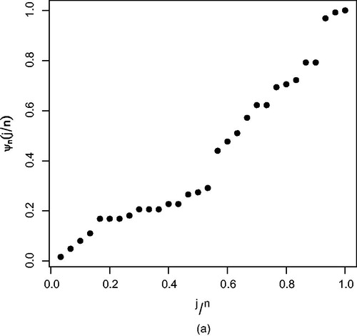
Table 7. Goodness of fit tests for different distributions.

Data set	Distribution	PDF	MLEs $(\widehat{{\theta }_1},\widehat{{\theta }_2})$	NLC	AIC	BIC	K-S
1	Lognormal	$f_X(x;\mu ,\tau )$	$(3.3581,1.7402)$	151.621	307.242	310.044	0.1047
	Weibull	$(k/\lambda ){(x/\lambda )}^{k-1}{e}^{-{(x/\lambda )}^k}$	$(0.8536,0.0183)$	151.937	307.874	310.676	0.1534
	Gamma	$[{\lambda }^k{x}^{k-1}{e}^{-\lambda x}]/\Gamma (k)$	$(0.8119,0.0136)$	152.167	308.369	311.171	0.1694
	GE	$k\lambda e^{-\lambda x}{(1-e^{-\lambda x})}^{k-1}$	$(0.8093,0.0145)$	152.201	308.401	311.204	0.1719
2	Lognormal	$f_X(x;\mu ,\tau )$	$(5.0750,0.0741)$	347.927	699.854	704.264	0.0489
	Weibull	$(k/\lambda ){(x/\lambda )}^{k-1}{e}^{-{(x/\lambda )}^k}$	$(3.7256,0.0054)$	353.292	710.584	714.993	0.0972
	Gamma	$[{\lambda }^k{x}^{k-1}{e}^{-\lambda x}]/\Gamma (k)$	$(13.538,0.0815)$	348.636	701.273	705.682	0.0516
	GE	$k\lambda e^{-\lambda x}{(1-e^{-\lambda x})}^{k-1}$	$(5.8404,0.0139)$	364.748	733.497	737.906	0.1493

We mention that this data set resembles the complete sample case with failure times of all n = 30 air conditioning systems of airplanes. Now, instead of considering the complete sample, we next generate a sample correspond to $n=30,m=22,T=85$ with the censoring scheme $(0^{*21},8)$, and get progressive type-II censored sample with the observations up to failure lifetime 71 and the rest are censored observations. Our purpose is to demonstrate that whether the censored observations are close to the predictive estimates obtained using various predictors. Also, our interest is to see that whether the predictive intervals contain censored observations or not. Now, based on the generated data set, we first report maximum likelihood, approximate maximum likelihood, and Bayes estimates in Table 8, and the associated 95% asymptotic confidence and HPD interval estimates in Table 9. We mention that Bayes estimates are obtained based on non-informative prior. From tabulated values it is observed that the estimated values of MLEs and AMLEs and Bayes estimates using Lindley and MH algorithm, are very close to each other. Further, the Bayes estimates obtained using LINEX loss with h = 1.5 have smaller estimated values which is followed by h = 0.5 and squared error Bayes estimates. We next report the predictive estimates for the first three censored observations in Table 10, and the associated predictive interval estimates in Table 11. The true observations are also reported in the tables. It is seen that the predictive estimates obtained using different predictors are quite close to the true observations. However, predictive estimates using MLP are smaller followed by the estimates of CMP and BUP. Further, predictive Bayes estimates under SEL have larger values as compared to Linex loss with h = 0.5 and h = 1.5. From Table 11, we observe that all prediction intervals contain the true values. It is also noticed that the interval estimates obtained using the HCD method have smaller intervals than those obtained using the pivotal method under classical approach, and further HPD prediction intervals are usually smaller compared to equal tail (ET) prediction intervals under Bayesian approach. It is further observed that all the intervals tend to become wider for higher order predicted values.

Table 8. Maximum likelihood and Bayes estimates of μ and τ for real data sets.

							Bayesian Estimation
					Classical		Lindley Method			Lindley Method			MH
Data					eEtimation		using AMLE			using MLE			Algorithm
set	(n, m)	Scheme	T		AMLE	MLE	SEL	LL^1	LL^2	SEL	LL^1	LL^2	SEL	LL^1	LL^2
1	(22, 30)	$(0^{*21},8)$	85	μ	3.404	3.405	3.424	3.406	3.370	3.426	3.407	3.372	3.426	3.406	3.365
				τ	1.976	1.976	2.274	2.184	1.973	2.277	2.187	1.976	2.306	2.152	1.948
2	(67, 40)	$(0^{*39},27)$	200	μ	5.070	5.072	5.074	5.073	5.072	5.074	5.074	5.073	5.069	5.068	5.067
				τ	0.072	0.070	0.077	0.076	0.075	0.076	0.075	0.074	0.066	0.066	0.064
	(72, 67)	$(0^{*66},5)$	300	μ	5.075	5.127	5.075	5.074	5.074	5.128	5.127	5.127	5.127	5.127	5.126
				τ	0.074	0.107	0.078	0.077	0.077	0.112	0.112	0.112	0.098	0.097	0.097

Note. LL¹ and LL² , respectively, correspond to h = 0.5 and h = 1.5 under LINEX loss.

Table 9. Asymptotic confidence and HPD interval estimates.

					Asymptotic CI		HPD Interval
Data set	(n, m)	Scheme	T		AMLE	MLE	MCMC
1	(22, 30)	$(0^{*21},8)$	85	μ	(2.874, 3.935)	(2.875, 3.934)	(2.879, 3.974)
				τ	(0.733, 3.219)	(0.735, 3.218)	(0.838, 3.944)
2	(67,40)	$(0^{*39},27)$	200	μ	(4.997, 5.148)	(4.999, 5.142)	(4.996, 5.138)
				τ	(0.036, 0.104)	(0.038, 0.103)	(0.047, 0.089)
	(72,67)	$(0^{*66},5)$	300	μ	(5.009, 5.140)	(5.052, 5.204)	(5.057, 5.199)
				τ	(0.049, 0.099)	(0.070, 0.144)	(0.070, 0.123)

Table 10. Point prediction.

						True	Classical Prediction			Bayesian Prediction
Data	(n, m)	Scheme	T	i	j	Value	MLP	BUP	CMP	SEL	LL^1	LL^2
1	(22, 30)	$(0^{*21},8)$	85	22	1	87	–	82.07	77.99	83.70	74.72	72.88
					2	90	81.46	95.94	90.57	99.91	78.59	74.82
					3	95	94.49	113.87	106.63	122.05	82.65	76.82
2	(67,40)	$(0^{*39},27)$	200	40	1	171	–	171.60	171.07	171.86	171.30	170.88
					2	172	171.67	173.24	172.72	175.44	173.40	172.14
					3	173	173.37	174.92	174.41	175.22	173.71	172.53
	(72,67)	$(0^{*66},5)$	300	T	1	NA	–	309.04	306.06	309.77	303.50	301.81
					2	NA	310.17	320.28	316.94	321.84	307.35	303.76
					3	NA	323.19	335.20	331.22	335.67	311.45	305.80

Note. – Represents that no suitable solution was found; NA- not available.

Table 11. Interval prediction.

						Classical Prediction		Bayesian Prediction
Data	(n, m)	Scheme	T	i	j	Pivotal	HCD	Credible	HPD
1	(22, 30)	$(0^{*21},8)$	85	22	1	(71.25, 114.64)	(71.00, 105.47)	(71.26, 125.02)	(71.00, 113.59)
					2	(73.67, 148.42)	(72.28, 126.85)	(73.70, 172.07)	(71.52, 150.77)
					3	(78.48, 190.74)	(76.85, 176.05)	(78.42, 239.73)	(74.82, 207.65)
2	(67,40)	$(0^{*39},27)$	200	40	1	(170.04, 176.20)	(170.00, 175.06)	(170.04, 177.01)	(170.00, 175.35)
					2	(170.40, 178.86)	(170.08, 177.63)	(169.44, 179.47)	(170.12, 179.17)
					3	(171.04, 181.58)	(170.58, 180.36)	(171.05, 182.97)	(170.52, 181.39)
	(72,67)	$(0^{*66},5)$	300	T	1	(300.23, 333.22)	(300.00, 327.02)	(300.24, 336.94)	(300.00, 328.85)
					2	(302.01, 346.03)	(301.71, 344.04)	(297.81, 362.92)	(300.49, 353.32)
					3	(304.73, 355.43)	(303.53, 350.24)	(307.11, 388.79)	(303.73, 378.30)

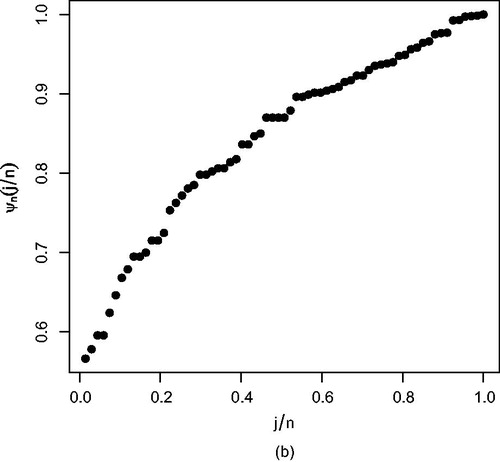
Data set 2. The second data set (see, Meeker and Escobar (2014), page-131) represents the number of cycles (in thousands) of fatigue life for 67 of 72 alloy T7987 specimens that failed before 300 thousand cycles. The observed data are,

94, 96, 99, 99, 104, 108, 112, 114, 117, 117, 118, 121, 121, 123, 129, 131,

133, 135, 136, 139, 139, 140, 141, 141, 143, 144, 149, 149, 152, 153, 159,

159, 159, 159, 162, 168, 168, 169, 170, 170, 171, 172, 173, 176, 177, 180,

180, 184, 187, 188, 189, 190, 196, 197, 203, 205, 211, 213, 224, 226, 227,

256, 257, 269, 271, 274, 291.

Figure 2 reports the TTT plot, and tabulated values from Table 7 suggest that lognormal distribution fits this data set well as compared to other considered distributions. We next generate a moderate sample of size 40 from the given data set correspond to $m=40,T=200$ thousand cycles with the censoring scheme $(0^{*39},27)$. Tables 8–11 report the estimates under classical and Bayesian approaches, associated interval estimates, predictive and associate predictive interval estimates. We observed the same behavior as mentioned in the previous section. However, in this case, we noticed that the 95% upper predictive bounds for the first three censored observations are also less than T = 200 thousand cycles. Therefore, if the experiment budget associated to a fixed time is available then this information may also help the experimenter to select the value of m accordingly.

Figure 2. Empirical scaled TTT transform for data set 2.

Observe that the data set 2 resembles the case of type-I censoring having $n=72,d=67$ and termination time T = 300 thousand cycles with five censored observations. Now we do not know the true values of the censored observations, and the predictive information from Tables 10 and 11 can be useful for the experimenter. From Table 8, we observed that with a higher sample size values of all estimates increase under classical and Bayesian approach, and further the lengths of associated interval estimates decrease(see Table 9). Also, the length of predictive intervals are smaller in the case of a large sample size, followed by moderate and small sample sizes.

7. Optimal Censoring

In previous sections, we considered problems of estimation and prediction for prescribed censoring schemes and taking into account prefixed time points, and we observed that the selection of different censoring schemes and times may lead to efficient estimates for unknown quantities of interest. Thus, selection of optimal plans and time points can be of important concerns to reliability practitioners. In the recent past, this problem has received much attention under different censoring methodologies, particularly progressive type-II censoring has been analyzed by several researchers. For instance, Ng et al. (2004) discussed D-optimality and A-optimality criteria for constructing optimal plans for a Weibull distribution, Pradhan and Kundu (2009) obtained optimal censoring schemes for a generalized exponential distribution based on optimizing the corresponding quantile function. However, the criterion based on pth quantile depends upon the value of $p,0<p<1,$. Later, Kundu (2008) proposed a more generalized criterion of the type optimizing ${\int }_0^{1}Var[\text{ln}\hspace{0.17em}{\widehat{X}}_p]W(p)dp$ where $\text{ln}\hspace{0.17em}{\widehat{X}}_p$ represents the logarithm of pth quantile and W(p) denotes a non-negative weight function, such that ${\int }_0^{1}W(p)dp=1$. Singh et al. (2015) also used this criterion for lognormal distribution and obtained sub-optimal censoring plans from the total possible schemes which belong to the convex hull generated by the points $(n-m,0,\dots ,0),\dots ,(0,0,\dots ,n-m)$. Observe that for a given value of n and m, a total of $(\begin{array}{c}n-1\\ m-1\end{array})$ choices are available to select a scheme $\mathrm{R}=(R_1,R-2,\dots ,R_m)$ such that ${\sum }_{i=1}^m{R}_i=(n-m)$. Thus, searching an optimal scheme among all possible schemes may be computationally inconvenient for higher values of n and m. Recently, Bhattacharya et al. (2016) proposed a meta heuristic based variable neighborhood search (VNS) algorithm which is quite useful in constructing optimal plans for moderate to large values of n and m. The main advantage of using VNS algorithm is that it provides near optimal solution with relatively less computation time. Construction of optimal plans under hybrid censoring is equivalent to selecting the values of m and T based on a given optimal criterion, and one may refer to Dube et al. (2011) for optimal hybrid censoring plans for a lognormal distribution. The objective of this section is to obtain optimal type-I progressive hybrid censoring plans for lognormal distribution. The construction of such plans under type-I progressive hybrid censoring is to select a scheme $\mathrm{R}$ and a time T for a given (n, m) based on a optimal criterion. We observed that selection of a time T is scale invariant and large time duration ca n be taken into account corresponding to a particular censoring scheme (see Bhattacharya et al.,2014). In this view, we next impose cost constraints like C_f, cost of each failed unit and C_t, operation cost for each time unit. So, the total cost associated with the experiment becomes $TC=C_{f}E(r)+C_{t}E(\mathcal{C})$. Here, E(r) and $E(\mathcal{C})$_, respectively, denote expected number of failures and expected duration of the experiment, and are given, respectively, by $$E\left(r\right)=\sum _{i=1}^m{F}_i(T,\theta )=m-\sum _{i=1}^m\sum _{j=1}^i{\sigma }_{i-1}\frac{a_{j,i}}{{\gamma }_j}{[1-F_X(T\left)\right]}^{{\gamma }_j},$$

and $$E\left(\mathcal{C}\right)=T{\sigma }_{m-1}\sum _{j=1}^m\frac{a_{j,m}}{{\gamma }_j}{[1-F_X(T\left)\right]}^{{\gamma }_j}+{\sigma }_{m-1}\sum _{j=1}^m{a}_{j,m}{\int }_{F_X\left(T\right)}^1{e}^{\mu +\sqrt{\tau }{\Phi }^{-1}\left(z\right)}{z}^{{\gamma }_j-1}dz.$$

The above expectations are computed with respect to the density as given in Equation (14)(14) $$f_i(x;\theta )={\sigma }_{i-1}\sum _{j=1}^i{a}_{j,i}\frac{1}{x\sqrt{\tau }}\varphi \left(\frac{\hspace{0.17em}\text{ln}\hspace{0.17em}x-\mu }{\sqrt{\tau }}\right){[1-\Phi (\frac{\hspace{0.17em}\text{ln}\hspace{0.17em}x-\mu }{\sqrt{\tau }}\left)\right]}^{{\gamma }_j-1},0<x<\infty ,$$(14) . One may further refer to Kundu and Joarder (2006) for more details on how to compute E(r). Also, the logarithmic of pth quantile is given by $\text{ln}\hspace{0.17em}{\widehat{X}}_p=\widehat{\mu }+\sqrt{\widehat{\tau }}{\Phi }^{-1}(p)$ where $\widehat{\mu }$ and $\widehat{\tau }$ denote maximum likelihood estimates of μ and τ, respectively. Therefore, construction of optimal plans under this criterion becomes equivalent to the optimization problem with cost constraints, and is given by, (13) $$\begin{array}{cccc}\hfill & \underset{(\mathrm{R},T)}{\text{Minimize}}\hfill & \hfill & {\int }_0^{1}Var(\text{ln}\hspace{0.17em}{\widehat{X}}_p)dp\hfill \\ \hfill & \text{Subject}\text{to}\hfill & \hfill & C_{f}E\left(r\right)+C_{t}E\left(\mathcal{C}\right)\le C_b.\hfill \end{array}$$(13)

Here, $${\int }_0^{1}Var(\text{ln}\hspace{0.17em}{\widehat{X}}_p)dp=l^{11}(\mathit{R},T)+\frac{l^{22}(\mathit{R},T)}{4\tau }{\int }_0^1({\Phi }^{-1}\left(p\right){)}^{2}dp+\frac{l^{12}(\mathit{R},T)}{\sqrt{\tau }}{\int }_0^1({\Phi }^{-1}\left(p\right))dp$$ where, $$\begin{array}{c}{l}^{11}(\mathit{R},T)=\frac{1}{\tau }\sum _{i=1}^m\sum _{j=1}^i{\sigma }_{i-1}{a}_{j,i}{\int }_0^{F\left(T\right)}({\Phi }^{-1}\left(t\right)-\frac{\varphi \left({\Phi }^{-1}\right(t\left)\right)}{1-t}{)}^2{(1-t)}^{{\gamma }_j-1}dt,\\ l^{22}(\mathit{R},T)=\frac{1}{4{\tau }^2}\sum _{i=1}^m\sum _{j=1}^i{\sigma }_{i-1}{a}_{j,i}{\int }_0^{F\left(T\right)}(1-{\left({\Phi }^{-1}\right(t\left)\right)}^2+{\Phi }^{-1}\left(t\right)\frac{\varphi \left({\Phi }^{-1}\right(t\left)\right)}{1-t}{)}^2{(1-t)}^{{\gamma }_j-1}dt,\end{array}$$ and $$\begin{array}{c}{l}^{12}(\mathit{R},T)=l^{21}(\mathit{R},T)=-\frac{1}{2{\tau }^{1.5}}\sum _{i=1}^m\sum _{j=1}^i{\sigma }_{i-1}{a}_{j,i}{\int }_0^{F\left(T\right)}(1-{\left({\Phi }^{-1}\right(t\left)\right)}^2+{\Phi }^{-1}(t\left)\frac{\varphi \left({\Phi }^{-1}\right(t\left)\right)}{1-t}\right)\\ \left({\Phi }^{-1}\right(t)-\frac{\varphi \left({\Phi }^{-1}\right(t\left)\right)}{1-t}){(1-t)}^{{\gamma }_j-1}dt.\end{array}$$

The elements, $l^{11}(.,.),l^{12}(.,.),l^{21}(.,.)$ and $l^{22}(.,.)$ of the Fisher information matrix are obtained from (see Park et al., 2011), $$I(\theta )={\int }_0^T{\{\frac{\partial }{\partial \theta }\text{ln}\hspace{0.17em}{h}_X(x,\theta \left)\right\}}^{\prime }\{\frac{\partial }{\partial \theta }\text{log}\hspace{0.17em}{h}_X(x\left)\right\}\sum _{i=1}^m{f}_i\left(x\right)dx$$ where $h_X(x,\theta )$ represents the hazard function of X , and $f_i(x,\theta )$ represent the PDF of the ith order statistics given by, (14) $$f_i(x;\theta )={\sigma }_{i-1}\sum _{j=1}^i{a}_{j,i}\frac{1}{x\sqrt{\tau }}\varphi \left(\frac{\hspace{0.17em}\text{ln}\hspace{0.17em}x-\mu }{\sqrt{\tau }}\right){[1-\Phi (\frac{\hspace{0.17em}\text{ln}\hspace{0.17em}x-\mu }{\sqrt{\tau }}\left)\right]}^{{\gamma }_j-1},0<x<\infty ,$$(14) with ${\gamma }_j=m-j+{\sum }_{l=j}^m{R}_l,{\sigma }_{i-1}={\prod }_{j=1}^i{\gamma }_j,i=1,2,\dots ,m$ and $a_{1,1}=1,a_{j,i}={\prod }_{l=1,l\ne j}^{i}1/({\gamma }_l-{\gamma }_j),1\le l\le i\le m$.

Next, we conduct a simulation study for different choices of (n, m) and total budget C_b along with the cost of failed units considered as C_f = 20 and the duration cost as C_t = 50. We employed the VNS algorithm and constructed optimal censoring schemes, and the results are reported in Table 12. We observed that when C_b increases the optimum values of T increase but the variance decreases. We mention that if one considers the C_p as the unit cost due to variance of the estimates of the unknown model parameters, available to the experimenter. Then, an alternative model which minimizes the total cost (TC) to obtain the optimum scheme can also be taken into account, $$TC=C_p{\int }_0^{1}Var(\text{ln}\hspace{0.17em}{\widehat{X}}_p)dp+C_{f}E\left(r\right)+C_{t}E\left(\mathcal{C}\right)$$ which is a unconstrained optimization problem, and one can use the VNS algorithm along with nlminb package in R-statistical language to obtain the desire optimum scheme $(\mathit{R},T)$. In Table 13, we report optimal censoring schemes based on this criterion with consideration of $C_f=10,C_t=25,C_p=250$. Notice that Lin et al. (2012) computed the optimum plan under Bayesian setup with fixed constraints using MCMC technique. Computation of such plans and, furthermore, consideration of plans with constraints also under a Bayesian setup, can be seen as future direction.

Table 12. Optimal censoring schemes and associated values of the criterion ${\int }_0^{1}Var(\text{ln}\hspace{0.17em}{\widehat{X}}_p)dp$.

		n = 20			n = 30			n = 40
m	Cb	$\mathit{R}$	T	Cri.	$\mathit{R}$	T	Cri.	$\mathit{R}$	T	Cri.
5	130	$(6,0^{*3},9)$	1.016	0.287	$(17,0^{*3},8)$	0.999	0.277	$(26,0^{*3},9)$	1.149	0.252
	150	$(10,0^{*2},2,3)$	3.711	0.253	$(21,0^{*3},4)$	10.24	0.242	$(31,0^{*3},4)$	10.24	0.198
8	180	$(3,0,1,0^{*4},8)$	0.901	0.169	$(13,0^{*4},1*2,7)$	1.024	0.185	$(18,3,0^{*5},11)$	0.796	0.176
	200	$(3,0^{*6},9)$	1.228	0.151	$(1,12,0^{*4},1,8)$	1.274	0.130	$(0,22,0,1,0^{*2},3,6)$	1.275	0.159
10	250	$(1,0,1,0^{*4},1,0,7)$	1.479	0.120	$(7,0,4,0^{*6},9)$	0.899	1.080	$(21,0^{*7},1,8)$	1.052	0.081
	270	$(0,5,0^{*7},5)$	2.546	0.097	$(14,0^{*6},2,0,4)$	2.567	0.089	$(24,0^{*8},6)$	10.24	0.098

Table 13. Optimal censoring schemes based on minimization of TC criterion.

	n = 20			n = 30			n = 40
m	$\mathrm{R}$	T	TC	$\mathrm{R}$	T	TC	$\mathrm{R}$	T	TC
5	$(5,0^{*3},10)$	1.6879	127.9226	$(15,0^{*3},10)$	1.6670	127.8180	$(25,0^{*3},10)$	1.6669	127.2455
8	$(7,0^{*6},5)$	0.8221	136.8608	$(17,0^{*6},5)$	0.7980	134.3990	$(27,0^{*6},5)$	0.7819	132.8223
10	$(7,0^{*7},1,2)$	0.8055	137.0688	$(16,1,0^{*7},3)$	0.7826	134.5867	$(27,0^{*8},3)$	0.7676	132.9938

8. Conclusion

In this article, we considered problems of estimation and prediction under classical and Bayesian approaches when lifetime data following a lognormal distribution are observed under type-I progressive hybrid censoring. We observed that maximum likelihood estimators (MLEs) of unknown parameters do not admit closed forms expressions. To compute these estimates, we employed an EM algorithm which has an advantage over the Newton-Raphson method but still requires an initial guess to implement. Therefore, we next obtained the approximate maximum likelihood estimators (AMLEs), and used these estimates as an initial guess for implementing the EM algorithm. In the simulation study, we also compared the performance of AMLEs with MLEs, and we observed that MLEs provide more efficient estimates than AMLEs. Similar behavior is noted in the comparison of corresponding asymptotic confidence intervals. Further, we obtained informative and non-informative Bayes estimates against squared error and LINEX loss functions. We first employed the Lindley method to compute these estimates. However, this method is not useful for interval estimation, and therefore, we next generated samples from the posterior densities using MH algorithm and constructed HPD intervals. In the simulation study, we found the performance of MH estimates quite satisfactory compared to the other proposed estimates. We mention that under the considered priors given by Equations (6)(6) $${\pi }^{*}(\mu ,\tau |x)\propto {\pi }^{*}(\mu ,\tau \left)L\right(\mu ,\tau \left|x\right),-\infty <\mu <\infty ,\tau >0.$$(6) and (7)(7) $$\pi (\mu ,\tau |x)=\frac{\pi (\tau )\times \pi (\mu |\tau )\times L(\mu ,\tau \left|x\right)}{{\int }_{-\infty }^{\infty }{\int }_0^{\infty }\pi (\tau )\times \pi (\mu |\tau )\times L(\mu ,\tau \left|x\right)d\tau d\mu },-\infty <\mu <\infty ,\tau >0.$$(7) , the corresponding posterior densities can also be written in the following form. $$\begin{array}{c}{\pi }^{*}(\mu ,\tau |x)\propto I{G}_{\tau }(\frac{r-1}{2},0.5\{\sum _{i=1}^r{(\text{ln}\hspace{0.17em}{x}_i)}^2-\frac{{({\sum }_{i=1}^r\hspace{0.17em}\text{ln}\hspace{0.17em}{x}_i)}^2}{r}\})\\ \times N_{\mu |\tau }(\frac{{\sum }_{i=1}^r\hspace{0.17em}\text{ln}\hspace{0.17em}{x}_i}{r},\frac{\tau }{r})\times H(\mu ,\tau ),\\ \pi (\mu ,\tau |x)\propto I{G}_{\tau }(\frac{r}{2}+p_2,0.5\{\sum _{i=1}^r{(\text{ln}\hspace{0.17em}{x}_i)}^2+a_1^2{b}_1+q_2-\frac{{({\sum }_{i=1}^r\hspace{0.17em}\text{ln}\hspace{0.17em}{x}_i+a_1{b}_1)}^2}{r+b_1}\})\\ \times N_{\mu |\tau }(\frac{{\sum }_{i=1}^r\hspace{0.17em}\text{ln}\hspace{0.17em}{x}_i+a_1{b}_1}{r+b_1},\frac{\tau }{r+b_1})\times H(\mu ,\tau ).\end{array}$$ where $H(\mu ,\tau )={\prod }_{i=1}^r(1-\Phi ({\xi }_i){)}^{R_i}{(1-\Phi ({\xi }_T))}^{R_T}$. Now, in both cases, the associated posterior densities are of type $I{G}_{\tau }(.,.)N_{\mu |\tau }(.,.)H(\mu ,\tau )$ and so one can also apply importance sampling procedure to obtain Bayes estimates. But, if we take independent prior distributions like $N_{\mu }(a_1,b_1)$ and $I{G}_{\tau }(p_2,q_2)$ for μ and τ in the present work, then for such consideration, the posterior density does not appear in a tractable form and so it becomes relatively difficult to use the importance sampling procedure. On the other hand, the proposed MH algorithm can still be applied. Next, we obtained prediction estimates of censored observations using maximum likelihood predictor, best unbiased predictor, conditional median predictor, and Bayesian predictors. Using the conditional density given by Equation (10)(10) $$f\left(z_{ij}\right|x,\mu ,\tau )=j\left(\begin{array}{c}{R}_i\\ j\end{array}\right)f(z_{ij}){\left[F\left(z_{ij}\right)-F\left({\mathcal{C}}^{*}\right)\right]}^{(j-1)}{\left[1-F\left(z_{ij}\right)\right]}^{(R_i-j)}{\left[1-F\left({\mathcal{C}}^{*}\right)\right]}^{-R_i},z_{ij}>{\mathcal{C}}^{*},$$(10) , we were able to construct predictive intervals using the pivotal method and the highest conditional density method. In the simulation study, we observed that HCD intervals provide smaller lengths compared to the pivotal intervals. Likewise, under the Bayesian approach, we observed that predictive highest posterior density intervals provide smaller interval lengths compared to the predictive equal tail intervals. In the data analysis, we found that all predictive estimates remain relatively close to the true observations, and also all the predictive intervals contain the true observations. Finally, we presented a discussion on optimal censoring using various optimality criteria. We established optimal plans with respect to cost constraints based on suggested optimal criterion, and reported results for different sampling situations.

Acknowledgements

The authors are thankful to two anonymous reviewers for their constructive suggestions that led to substantial improvements in the earlier version of this manuscript. Authors also extend their sincere thanks to the Editor and the Associate Editor for some very useful suggestions.

References

- Aarset, M. V. (1987). How to identify a bathtub hazard rate. IEEE Transactions on Reliability, R-36(1), 106–108.
- Asl, M. N., Belaghi, R. A., & Bevrani, H. (2017). On Burr XII distribution analysis under progressive type-ii hybrid censored data. Methodology and Computing in Applied Probability, 19(2), 665–683.
- Balakrishnan, N., & Cramer, E. (2014). Art of Progressive Censoring. Berlin, Germany: Springer.
- Balakrishnan, N., Kannan, N., Lin, C.-T., & Ng, H. T. (2003). Point and interval estimation for gaussian distribution based on progressively type-ii censored samples. IEEE Transactions on Reliability, 52(1), 90–95.
- Balakrishnan, N., & Mi, J. (2003). Existence and uniqueness of the MLES for normal distribution based on general progressively Type-II censored samples. Statistics & Probability Letters, 64(4), 407–414.
- Bhattacharya, R., Pradhan, B., & Dewanji, A. (2014). Optimum life testing plans in presence of hybrid censoring: A cost function approach. Applied Stochastic Models in Business and Industry, 30(5), 519–528.
- Bhattacharya, R., Pradhan, B., & Dewanji, A. (2016). On optimum life-testing plans under Type-II progressive censoring scheme using variable neighborhood search algorithm. TEST, 25(2), 309–330.
- Chen, M.-H., & Shao, Q.-M. (1999). Monte Carlo estimation of Bayesian credible and HPD intervals. Journal of Computational and Graphical Statistics, 8(1), 69–92.
- Cohen, A. C. (1965). Maximum likelihood estimation in the Weibull distribution based on complete and on censored samples. Technometrics, 7(4), 579–588.
- Cramer, E., & Balakrishnan, N. (2013). On some exact distributional results based on Type-I progressively hybrid censored data from exponential distributions. Statistical Methodology, 10(1), 128–150.
- Dey, S., Singh, S., Tripathi, Y. M., & Asgharzadeh, A. (2016). Estimation and prediction for a progressively censored generalized inverted exponential distribution. Statistical Methodology, 32, 185–202.
- Dube, S., Pradhan, B., & Kundu, D. (2011). Parameter estimation of the hybrid censored log-normal distribution. Journal of Statistical Computation and Simulation, 81(3), 275–287.
- Golparvar, L., & Parsian, A. (2016). Inference on proportional hazard rate model parameter under type-i progressively hybrid censoring scheme. Communications in Statistics-Theory and Methods, 45(24), 7258–7274.
- Hemmati, F., & Khorram, E. (2013). Statistical analysis of the log-normal distribution under Type-II progressive hybrid censoring schemes. Communications in Statistics-Simulation and Computation, 42(1), 52–75.
- Kundu, D. (2008). Bayesian inference and life testing plan for the Weibull distribution in presence of progressive censoring. Technometrics, 50(2), 144–154.
- Kundu, D., & Joarder, A. (2006). Analysis of type-ii progressively hybrid censored data. Computational Statistics and Data Analysis, 50(10), 2509–2528.
- Lin, C. T., Chou, C. C., & Huang, Y. L. (2012). Inference for the Weibull distribution with progressive hybrid censoring. Computational Statistics and Data Analysis, 56(3), 451–467.
- Lindley, D. V. (1980). Approximate Bayesian methods. Trabajos De Estadística y De Investigación Operativa, 31(1), 223–245.
- Linhardt, H., & Zucchin, W. (1986). Model Selection. New York, NY: Wiley.
- Louis, T. A. (1982). Finding the observed information matrix when using the EM algorithm. Journal of the Royal Statistical Society. Series B (Methodological), 226–233.
- Meeker, W. Q., & Escobar, L. A. (2014). Statistical methods for reliability data. Hoboken, NJ: John Wiley & Sons.
- Ng, H., Chan, P., & Balakrishnan, N. (2002). Estimation of parameters from progressively censored data using EM algorithm. Computational Statistics & Data Analysis, 39(4), 371–386.
- Ng, H., Chan, P., & Balakrishnan, N. (2004). Optimal progressive censoring plans for the Weibull distribution. Technometrics, 46(4), 470–481.
- Park, S., Balakrishnan, N., & Kim, S. W. (2011). Fisher information in progressive hybrid censoring schemes. Statistics, 45(6), 623–631.
- Pradhan, B., & Kundu, D. (2009). On progressively censored generalized exponential distribution. Test, 18(3), 497–515.
- Raqab, M. Z., & Nagaraja, H. (1995). On some predictors of future order statistics. Metron, 53(12), 185–204.
- Singh, S., & Tripathi, Y. M. (2016). Bayesian estimation and prediction for a hybrid censored lognormal distribution. IEEE Transactions on Reliability, 65(2), 782–795.
- Singh, S., Tripathi, Y. M., & Wu, S.-J. (2015). On estimating parameters of a progressively censored lognormal distribution. Journal of Statistical Computation and Simulation, 85(6), 1071–1089.
- Tomer, S. K., & Panwar, M. (2015). Estimation procedures for Maxwell distribution under Type-I progressive hybrid censoring scheme. Journal of Statistical Computation and Simulation, 85(2), 339–356.
- Turkkan, N., & Pham-Gia, T. (1993). Computation of the highest posterior density interval in bayesian analysis. Journal of Statistical Computation and Simulation, 44(3-4), 243–250.