Estimation and Prediction for the Power-Exponential Hazard Rate Distribution Based on Record Data

Synoptic Abstract

The problems of classical and Bayesian estimation of the parameters of the power-exponential hazard rate distribution (P-EHRD) based on record values and the prediction of future record values are considered. The parameters of P-EHRD are estimated by the maximum likelihood and the least squares methods, and the Bayes estimates are obtained by the Metropolis-Hastings method under the squared error loss and LINEX loss functions. Also, an asymptotic confidence interval, two bootstrap confidence intervals and the highest posterior density (HPD) credible interval for the unknown parameters are constructed. The problem of predicting the future record values from the P-EHRD based on the past record values is considered using the maximum likelihood and Bayesian approaches. To investigate and compare the performance of the different proposed methods, a Monte Carlo simulation study is conducted. Finally, an example is presented to illustrate the estimation and prediction procedures.

KEY WORDS AND PHRASES:

• Bayes estimation
• bootstrap confidence intervals
• least squares estimation
• power-exponential hazard rate distribution
• prediction
• record values

1. Introduction

Record values arise naturally in many real life applications, such as climatology, sports, economics, life tests and so on. For example, it might be interesting to a researcher in a manufacturing industry to determine the minimum failure stress of the product sequentially, while the amount of the rainfall that is greater (smaller) than the previous ones is of importance to climatologists and hydrologists. For more examples and details, see Arnold, Balakrishnan, and Nagaraja (1998).

Let $\{X_i,i\ge 1\}$ be a sequence of independent and identically distributed (iid) random variables with an absolutely continuous cumulative distribution function (cdf), F(x), and probability density function (pdf), f(x). An observation X_j is called an upper record if its value exceeds all previous observations, i.e. X_j is an upper record if $X_j>X_i$ for every i < j. The record time sequence $\{T_n,n\ge 1\},$ at which the records appear, is defined as, $$T_n=\min \{j:j>T_{n-1},X_j>X_{T_{n-1}}\},\hspace{1em}n>1,$$ and $T_1=1$ with probability 1. Then, the sequence of upper record values is defined by $R_n=X_{T_n},n\ge 1.$ An analogous definition can be given for lower records. It is important to note that there are two sampling schemes for generating record data: the random sampling scheme and the inverse sampling scheme. Under the random sampling scheme, a random sample $X_1,\dots ,X_n$ is examined sequentially and successive maximum values are recorded, while under the inverse sampling scheme, units are taken sequentially and sampling is terminated when a prespecified number of record values m are observed. These sampling schemes play an important role in statistical inference when one considers record values with inter-record times.

Chandler (1952) first introduced the topic of record values and studied their basic properties. Since then, such ordered data has been studied extensively in the literature. The problem of making inference based on record observations from a particular distribution has received attention of many researchers, and for literature on this topic one may refer to Soliman, Abd Ellah, and Sultan (2006) for the Weibull distribution, Asgharzadeh and Fallah (2011) for the exponentiated family of distributions, Dey, Dey, Salehi, and Ahmadi (2013) for the generalized exponential distribution, Kumar, Kumar, Saran, and Jain (2017) for the Kumaraswamy-Burr III distribution, Asgharzadeh, Fallah, Raqab, and Valiollahi (2018) for the Lindley distribution, Raqab, Bdair, and Al-Aboud (2018) for the two-parameter bathtub-shaped distribution, and Pak and Dey (2019) for the power Lindley distribution.

The hazard rate function is an important characteristic of lifetime distributions, since it describes the instantaneous failure rate at any time and is a useful tool to monitor the lifetime of a unit in life testing and reliability studies. If the lifetime of a unit is described by a random variable X with pdf f(x) and cdf F(x), then the hazard rate function h(x) is defined by $$h(x)=\frac{f(x)}{1-F(x)}.$$ Lifetime distributions are often specified by choosing a particular hazard rate function in reliability theory. In this regard, the linear hazard rate function ($h(x)=a+\mathit{bx},x>0,a,b\ge 0$) by Bain (1974), the power hazard rate function ($h(x)=a{x}^k,x>0,a>0,k>-1$) by Mugdadi (2005) and the exponential hazard rate function ($h(x)=a{e}^{\mathit{cx}},x>0,a,c>0$) by Gompertz (1825) were considered by some researchers. Unfortunately, these hazard rate functions are monotone and therefore they do not provide a reasonable parametric fit for modeling phenomenon with bathtub-shaped hazard rates which are common in biological and reliability studies. Recently, Tarvirdizade and Nematollahi (2019) introduced a more general hazard rate function by combining the power hazard rate function and the exponential hazard rate function. This is the power-exponential hazard rate function, defined as (1) $$h(x)=a{x}^k+b{e}^{\mathit{cx}},\hspace{1em}x>0,\hspace{1em}a,b,c\ge 0,\hspace{1em}k>-1,$$(1) where a, b, c and k are the parameters such that $a+b>0.$ The power-exponential hazard rate function can cover bathtub-shaped case when $a,b,c>0$ and k < 0. The cdf and the pdf corresponding to this hazard rate function are given by (2) $$F(x)=1-\hspace{0.17em}\text{exp}\hspace{0.17em}\left\{\frac{-a}{k+1}{x}^{k+1}-\frac{b}{c}(e^{\mathit{cx}}-1)\right\},\hspace{1em}x>0,\hspace{1em}a,b,c\ge 0,\hspace{1em}k>-1,$$(2) and (3) $$f(x)=(a{x}^k+b{e}^{\mathit{cx}})\hspace{0.17em}\text{exp}\hspace{0.17em}\left\{\frac{-a}{k+1}{x}^{k+1}-\frac{b}{c}(e^{\mathit{cx}}-1)\right\},\hspace{1em}x>0,\hspace{1em}a,b,c\ge 0,\hspace{1em}k>-1,$$(3) respectively. This distribution is called the power-exponential hazard rate distribution (P-EHRD). The exponential, Rayleigh, Weibull, modified Weibull, Gompertz, Gompertz-Makeham, linear hazard rate and power hazard rate distributions are the most important sub-models of the P-EHRD. Some distributional properties and estimation of the parameters based on a complete sample for the P-EHRD were studied by Tarvirdizade and Nematollahi (2019). They have also showed that the P-EHRD provides a better fit than other four-parameter distributions for data with a bathtub-shaped hazard rate while its hazard rate function is very simple in comparison with those of the competitor distributions.

To the best of our knowledge, inference based on record data from the P-EHRD is not available in the literature. Because of the importance of record values in many fields of application and since the P-EHRD can be used quite effectively in analyzing the lifetime data, especially the data with a bathtub-shaped hazard rate, in this paper the record values are used to estimate the parameters of the P-EHRD and predict the future record values for this distribution. First the maximum likelihood estimates of the parameters are obtained, which then are used to construct asymptotic and bootstrap confidence intervals. Next, the least squares method is used for estimating the parameters of the P-EHRD, and the Bayes estimates of the parameters based on symmetric and asymmetric loss functions are obtained. The HPD credible intervals for the parameters are constructed using random samples generated from the MCMC method. The prediction of future record values based on the observed upper record values from the P-EHRD is discussed. An example is used to demonstrate the application of inference techniques and a simulation study is conducted to compare different methods of estimation and prediction.

The rest of the paper is organized as follows. In Section 2, the maximum likelihood (ML) and the least squares (LS) methods are used for estimating the parameters of the P-EHRD based on upper record values. The asymptotic confidence intervals and two bootstrap confidence intervals for the parameters of the P-EHRD are also considered. In Section 3, the Bayes estimates of unknown parameters under the squared error (SE) and linear-exponential (LINEX) loss functions via the Metropolis-Hastings method are obtained, and the HPD credible interval for the parameters are constructed. The problem of predicting the future record values from the P-EHRD is considered using the ML and Bayesian approaches in Sections 4 and 5, respectively. In Section 6, an example is presented to illustrate the estimation and prediction procedures discussed in the previous sections. To investigate and compare the performance of the different methods of estimation and prediction presented in this paper, outcomes of a Monte Carlo simulation study are also presented. Finally, some conclusions are provided in Section 7.

2. Classical Estimation

The ML estimates of the parameters of the P-EHRD based on upper record values are obtained in this section and then used them to construct asymptotic and bootstrap confidence intervals. The LS method for estimating the parameters of the P-EHRD is also presented.

2.1. Maximum Likelihood Estimation

Let $\underset{\sim }{r}=(r_1,\dots ,r_n)$ be the first n upper record values observed from a population with cdf F(x) and pdf f(x). The joint density function of the first n upper record values is given by (Ahsanullah, 2004), (4) $$f(\underset{\sim }{r})=f(r_n)\prod _{i=1}^{n-1}\left(\frac{f(r_i)}{1-F(r_i)}\right),\hspace{1em}-\infty <r_1<\dots <r_n<\infty .$$(4)

From (4(4) $$f(\underset{\sim }{r})=f(r_n)\prod _{i=1}^{n-1}\left(\frac{f(r_i)}{1-F(r_i)}\right),\hspace{1em}-\infty <r_1<\dots <r_n<\infty .$$(4) ) with F and f replaced by (2(2) $$F(x)=1-\hspace{0.17em}\text{exp}\hspace{0.17em}\left\{\frac{-a}{k+1}{x}^{k+1}-\frac{b}{c}(e^{\mathit{cx}}-1)\right\},\hspace{1em}x>0,\hspace{1em}a,b,c\ge 0,\hspace{1em}k>-1,$$(2) ) and (3(3) $$f(x)=(a{x}^k+b{e}^{\mathit{cx}})\hspace{0.17em}\text{exp}\hspace{0.17em}\left\{\frac{-a}{k+1}{x}^{k+1}-\frac{b}{c}(e^{\mathit{cx}}-1)\right\},\hspace{1em}x>0,\hspace{1em}a,b,c\ge 0,\hspace{1em}k>-1,$$(3) ), respectively, it follows that the likelihood function is given by (5) $$L(a,b,c,k|\underset{\sim }{r})=\prod _{i=1}^n(a{r}_i^k+b{e}^{c{r}_i})\hspace{0.17em}\text{exp}\hspace{0.17em}\left\{-\frac{a}{k+1}{r}_n^{k+1}-\frac{b}{c}(e^{c{r}_n}-1)\right\},0<r_1<\dots <r_n<\infty .$$(5) Now taking partial derivatives the log-likelihood function with respect to $(a,b,c,k),$ the likelihood equations can be obtained as follows (6) $$\frac{\partial \ell }{\partial a}=\sum _{i=1}^n\frac{r_i^k}{a{r}_i^k+b{e}^{c{r}_i}}-\frac{1}{k+1}{r}_n^{k+1}=0,$$(6) (7) $$\frac{\partial \ell }{\partial b}=\sum _{i=1}^n\frac{e^{c{r}_i}}{a{r}_i^k+b{e}^{c{r}_i}}-\frac{1}{c}(e^{c{r}_n}-1)=0,$$(7) (8) $$\frac{\partial \ell }{\partial c}=\sum _{i=1}^n\frac{b{r}_i{e}^{c{r}_i}}{a{r}_i^k+b{e}^{c{r}_i}}-\frac{b}{c^2}(c{r}_n{e}^{c{r}_n}-e^{c{r}_n}+1)=0,$$(8) (9) $$\frac{\partial \ell }{\partial k}=\sum _{i=1}^n\frac{a{r}_i^k\hspace{0.17em}\text{log}\hspace{0.17em}{r}_i}{a{r}_i^k+b{e}^{c{r}_i}}-\frac{a}{{(k+1)}^2}{r}_n^{k+1}\left[(k+1)\hspace{0.17em}\text{log}\hspace{0.17em}{r}_n-1\right]=0.$$(9) Using (6(6) $$\frac{\partial \ell }{\partial a}=\sum _{i=1}^n\frac{r_i^k}{a{r}_i^k+b{e}^{c{r}_i}}-\frac{1}{k+1}{r}_n^{k+1}=0,$$(6) ) and (7(7) $$\frac{\partial \ell }{\partial b}=\sum _{i=1}^n\frac{e^{c{r}_i}}{a{r}_i^k+b{e}^{c{r}_i}}-\frac{1}{c}(e^{c{r}_n}-1)=0,$$(7) ), we can obtain a as a function of b, c and k as (10) $$a=g(b,c,k)=\frac{(k+1)\left(n-\frac{b}{c}(e^{c{r}_n}-1)\right)}{r_n^{k+1}}$$(10) By replacing (10(10) $$a=g(b,c,k)=\frac{(k+1)\left(n-\frac{b}{c}(e^{c{r}_n}-1)\right)}{r_n^{k+1}}$$(10) ) into (7)–(9), we get the following system of nonlinear equations (11) $$\frac{\partial \ell }{\partial b}=\sum _{i=1}^n\frac{e^{c{r}_i}}{g(b,c,k)r_i^k+b{e}^{c{r}_i}}-\frac{1}{c}(e^{c{r}_n}-1)=0,$$(11) (12) $$\frac{\partial \ell }{\partial c}=\sum _{i=1}^n\frac{b{r}_i{e}^{c{r}_i}}{g(b,c,k)r_i^k+b{e}^{c{r}_i}}-\frac{b}{c^2}(c{r}_n{e}^{c{r}_n}-e^{c{r}_n}+1)=0,$$(12) (13) $$\frac{\partial \ell }{\partial k}=\sum _{i=1}^n\frac{g(b,c,k)r_i^k\hspace{0.17em}\text{log}\hspace{0.17em}{r}_i}{g(b,c,k)r_i^k+b{e}^{c{r}_i}}-\frac{g(b,c,k)}{{(k+1)}^2}{r}_n^{k+1}\left[(k+1)\hspace{0.17em}\text{log}\hspace{0.17em}{r}_n-1\right]=0.$$(13) By solving (11)–(13) with respect to b, c and k, the ML estimates of the parameters, say $\widehat{b},\widehat{c}$ and $\widehat{k},$ respectively, can be obtained. These equations are very complicated and cannot be solved analytically. Therefore, a numerical iteration method such as Newton-Raphson method is recommended to solve these simultaneous equations to obtain $\widehat{b},\widehat{c}$ and $\widehat{k}.$ Then substituting $\widehat{b},\widehat{c}$ and $\widehat{k}$ in place of b, c and k in (10(10) $$a=g(b,c,k)=\frac{(k+1)\left(n-\frac{b}{c}(e^{c{r}_n}-1)\right)}{r_n^{k+1}}$$(10) ), the ML estimate of a, say $\widehat{a},$ can be obtained. The subroutines to solve non-linear optimization problem are available in R software. We used nlm() package for this purpose. For maximizing the log-likelihood function, the nlm function was executed for a wide range of initial values. This procedure usually leads to more than one maximum. In such cases, the MLEs corresponding to the largest value of the maxima is used. For a few initial values, no maximum was identified, in such cases, a new initial value was used to obtain a maximum.

2.2. Asymptotic Confidence Intervals

Since the exact sampling distribution of the ML estimates cannot be obtained in closed form, the approximate confidence intervals are obtained for the parameters a, b, c, and k by using the approximate distributions of their ML estimates which is need to calculate the Fisher information matrix. The observed information matrix is computed since the expected information matrix is too complicated and requires numerical integration. The elements of the 4 × 4 observed information matrix I are given in the Appendix. The asymptotic distribution of the ML estimators of the parameters a, b, c, and k are given by (see Miller, 1981) (14) $$\left(\widehat{a},\widehat{b},\widehat{c},\widehat{k}\right)\sim N_4\left((a,b,c,k),\mathbf{V}\right),$$(14) where V is the variance-covariance matrix and can be approximated by the reciprocal of the observed information matrix I, i.e., $\mathbf{V}=I^{-1},$ which involves the unknown parameters a, b, c, and k. Since the ML estimators are consistent estimators, the parameters are replaced by the corresponding ML estimates in order to obtain an estimate of V, which is given by (15) $$\widehat{V}=\left(\begin{array}{cccc}{\widehat{V}}_{11}& {\widehat{V}}_{12}& {\widehat{V}}_{13}& {\widehat{V}}_{14}\\ {\widehat{V}}_{21}& {\widehat{V}}_{22}& {\widehat{V}}_{23}& {\widehat{V}}_{24}\\ {\widehat{V}}_{31}& {\widehat{V}}_{32}& {\widehat{V}}_{33}& {\widehat{V}}_{34}\\ {\widehat{V}}_{41}& {\widehat{V}}_{42}& {\widehat{V}}_{43}& {\widehat{V}}_{44}\end{array}\right)={\left(\begin{array}{cccc}{\widehat{I}}_{11}& {\widehat{I}}_{12}& {\widehat{I}}_{13}& {\widehat{I}}_{14}\\ {\widehat{I}}_{21}& {\widehat{I}}_{22}& {\widehat{I}}_{23}& {\widehat{I}}_{24}\\ {\widehat{I}}_{31}& {\widehat{I}}_{32}& {\widehat{I}}_{33}& {\widehat{I}}_{34}\\ {\widehat{I}}_{41}& {\widehat{I}}_{42}& {\widehat{I}}_{43}& {\widehat{I}}_{44}\end{array}\right)}^{-1},$$(15) where ${\widehat{I}}_{\mathit{ij}}$ is the (i, j)th element of the observed information matrix I with a, b, c and k replaced by $\widehat{a},\widehat{b},\widehat{c},$ and $\widehat{k},$ respectively. Now, using (14(14) $$\left(\widehat{a},\widehat{b},\widehat{c},\widehat{k}\right)\sim N_4\left((a,b,c,k),\mathbf{V}\right),$$(14) ), the $100(1-\alpha )\%$ approximate confidence intervals for the parameters a, b, c, and k are given, respectively, by (16) $$\widehat{a}\pm z_{\alpha /2}\sqrt{{\widehat{V}}_{11}},\hspace{1em}\widehat{b}\pm z_{\alpha /2}\sqrt{{\widehat{V}}_{22}},\hspace{1em}\widehat{c}\pm z_{\alpha /2}\sqrt{{\widehat{V}}_{33}},\hspace{1em}\mathrm{and}\hspace{1em}\widehat{k}\pm z_{\alpha /2}\sqrt{{\widehat{V}}_{44}},$$(16) where $z_{\alpha /2}$ is the $(1-\alpha /2)$th quantile of the standard normal distribution.

According to Arnold et al. (1998), records are rare in practice and so anyone developing inferential techniques involving record values will usually be faced with small samples. Therefore, confidence intervals based on the asymptotic results are expected not to perform very well. In such situations, one can use some resampling techniques to provide more accurate approximate confidence intervals. Here, two bootstrap confidence intervals are proposed and the performance of the various approximate intervals for different sample sizes are compared in Section 6 using their coverage probability and expected length.

2.3. Bootstrap Confidence Intervals

In this subsection, two bootstrap resampling method to find approximate confidence intervals for the parameters a, b, c and k of P-EHRD are proposed. The first is the percentile bootstrap (Boot-p) confidence interval based on the idea of Efron (1982), and the second is the student’s t bootstrap (Boot-t) confidence interval based on the idea of Hall (1988). First, generate the upper record samples from P-EHRD using the algorithm suggested in Arnold et al. (1998) to generate n independent samples $x_1^{*},x_2^{*},\dots ,x_n^{*}$ from the standard exponential distribution, Exp(1(1) $$h(x)=a{x}^k+b{e}^{\mathit{cx}},\hspace{1em}x>0,\hspace{1em}a,b,c\ge 0,\hspace{1em}k>-1,$$(1) ) and solving the following equation for given values of the parameters a, b, c and k: $$\frac{a}{k+1}{r}_i^{k+1}+\frac{b}{c}\left(e^{c{r}_i}-1\right)-\sum _{j=1}^i{x}_j^{*}=0,\hspace{1em}i=1,2,\dots ,n.$$ Then $r_1,r_2,\dots ,r_n$ are the required upper record samples from the P-EHRD. As suggested by Efron and Tibshirani (1993), the following algorithm is used to generate parametric bootstrap samples.

Algorithm 1

Step 1. Compute $\widehat{a},\widehat{b},\widehat{c},$ and $\widehat{k},$ the ML estimates of the parameters a, b, c, and k based on the upper record samples $\underset{\sim }{r}=(r_1,\dots ,r_n).$

Step 2. Generate the bootstrap upper record samples ${\underset{\sim }{r}}^{*}=(r_1^{*},r_2^{*},\dots ,r_n^{*})$ from the P-EHRD with the parameters $\widehat{a},\widehat{b},\widehat{c},$ and $\widehat{k}$ by using the method described before Algorithm 1. From these data, compute the bootstrap estimates say, ${\widehat{a}}^{*},{\widehat{b}}^{*},{\widehat{c}}^{*},$ and ${\widehat{k}}^{*}.$

Step 3. Repeat step 2, B times to obtain a set of bootstrap samples of a, b, c, and k, say $({\widehat{a}}_1^{*},\dots ,{\widehat{a}}_B^{*}),({\widehat{b}}_1^{*},\dots ,{\widehat{b}}_B^{*}),({\widehat{c}}_1^{*},\dots ,{\widehat{c}}_B^{*})$ and $({\widehat{k}}_1^{*},\dots ,{\widehat{k}}_B^{*}).$

To construct the bootstrap confidence intervals of the parameter θ (which is a, b, c or k), the bootstrap samples generated by Algorithm 1 are used, and two different bootstrap confidence intervals are obtained as follows:

(I) Boot-p method

Let $G(x)=\mathit{Pr}({\widehat{\theta }}^{*}\le x)$ be the cdf of ${\widehat{\theta }}^{*}.$ Define ${\widehat{\theta }}_{\mathit{Boot}}(x)=G^{-1}(x)$ for a given x. Then the $100(1-\alpha )\%$ bootstrap percentile interval for θ is defined by (17) $$\left({\widehat{\theta }}_{\mathit{Boot}}\left(\frac{\alpha }{2}\right),{\widehat{\theta }}_{\mathit{Boot}}\left(1-\frac{\alpha }{2}\right)\right),$$(17) which are the $(\alpha /2)$th and $(1-\alpha /2)$ th quantiles of the bootstrap sample $\widehat{{\theta }_1^{*}},\dots ,\widehat{{\theta }_B^{*}}.$

(II) Boot-t method

Let $$T_b^{*}=\frac{({\widehat{\theta }}_i^{*}-\widehat{\theta })}{\widehat{s}{e}_i^{*}},\hspace{1em}i=1,2,\dots ,B,$$ where $\widehat{s}{e}_i^{*}$ is an estimate of the standard error of ${\widehat{\theta }}_i^{*}$ and can be replaced by its asymptotic standard error. Then the $100(1-\alpha )\%$ bootstrap student’s t interval is given by (18) $$(\widehat{\theta }-t_{1-\alpha /2}^{*}\widehat{s}{e}_{\mathit{boot}},\widehat{\theta }-t_{\alpha /2}^{*}\widehat{s}{e}_{\mathit{boot}}),$$(18) where $t_{\alpha }^{*}$ is the αth quantile of $T_1^{*},\dots ,T_B^{*}$ and $\widehat{s}{e}_{\mathit{boot}}$ is the bootstrap estimate of the standard error based on $\widehat{{\theta }_1^{*}},\dots ,\widehat{{\theta }_B^{*}}.$

2.4. Least Squares Estimation

For estimation of the parameters of Beta distribution under the complete sample, Swain, Venkatraman, and Wilson (1988) introduced the least squares (LS) estimation. Then, several authors used this method to estimate the parameters of some distributions under censored and record data, for example, Lin, Wu, and Balakrishnan (2003) and Krishna and Kumar (2013). In this subsection, this method is used to estimate the parameters of P-EHRD based on upper record values. Let $\underset{\sim }{r}=(r_1,\dots ,r_n)$ be the first n upper record values observed from a population with cdf F(x) and pdf f(x). Then, the LS estimates of the parameters can be obtained by minimizing $$Q=\sum _{i=1}^n{\left(F(r_i)-E[F(r_i)]\right)}^2$$ with respect to the parameters. The marginal pdf of $R_i,$ for $i=1,2,\dots ,n,$ is given by (Ahsanullah, 2004) $$f_{R_i}(r_i)=\frac{1}{(i-1)!}f(r_i){\left(-\hspace{0.17em}\text{log}[1-F(r_i)]\right)}^{i-1}.$$

Thus, it can be easily shown that $$E[F(r_i)]=1-\frac{1}{2^i}.$$

Now, for the P-EHRD, the LS estimates of the parameters can be obtained by minimizing (19) $$Q=\sum _{i=1}^n{\left(\frac{1}{2^i}-\hspace{0.17em}\text{exp}\hspace{0.17em}\left\{-\frac{a}{k+1}{r}_i^{k+1}-\frac{b}{c}(e^{c{r}_i}-1)\right\}\right)}^2$$(19) with respect to the parameters a, b, c, and k. Thus, the LS estimates of the parameters a, b, c, and k are the solutions of the simultaneous equations obtained from the partial derivatives (19(19) $$Q=\sum _{i=1}^n{\left(\frac{1}{2^i}-\hspace{0.17em}\text{exp}\hspace{0.17em}\left\{-\frac{a}{k+1}{r}_i^{k+1}-\frac{b}{c}(e^{c{r}_i}-1)\right\}\right)}^2$$(19) ) with respect to the parameters a, b, c, and k. Since these equations are complicated function of the parameters a, b, c, and k, they are difficult to solve analytically. Instead, iterative techniques such as a Newton-Raphson can be used to obtain the LS estimates of the parameters a, b, c and k, say ${\tilde{a}}_{\mathit{LS}},{\tilde{b}}_{\mathit{LS}},{\tilde{c}}_{\mathit{LS}},$ and ${\tilde{k}}_{\mathit{LS}},$ respectively.

3. Bayes Estimation

One of the attractive methods of estimation of the parameters of a distribution is the Bayes estimation. In this method, for estimation the parameter θ by the estimator $\delta (X),$ the researcher needs a prior distribution, $\pi (\theta ),$ for θ, as well as a loss function, $L(\theta ,\delta (X)),$ for estimation process. The Bayes estimate of θ is obtained by minimizing the posterior risk $\rho (x,\delta (x))=E\left[L(\theta ,\delta (x))|x\right]$ with respect to θ.

In literature, for simplicity, the squared error (SE) loss function $L(\theta ,\delta (X))={(\delta (X)-\theta )}^2$ is used for estimation problems. Under the SE loss function, the Bayes estimator of θ is given by ${\delta }_{\mathit{BS}}(X)=E(\theta |\mathbf{X}).$ This loss function is convex and symmetric, and assigns equal losses to the overestimation and underestimation. However, in some practical situations overestimation may by more serious than underestimation or vice versa. For example, overestimation is usually more serious than underestimation in the estimation of reliability and hazard rate functions. In these cases, the use of symmetric loss functions may be inappropriate. Instead, the use of an asymmetric loss function which assigns greater importance to overestimation or underestimation may be more appropriate. Varian (1975) proposed an asymmetric linear-exponential loss function known as LINEX loss function which is given by (20) $$L(\theta ,\delta )=e^{d(\delta -\theta )}-d(\delta -\theta )-1,\hspace{1em}d\ne 0,$$(20) where the shape parameter d is known and gives the degree of asymmetry. If d >  0, the overestimation is more serious than underestimation and if d <  0, underestimation is more serious than overestimation. If d close to zero, the LINEX loss function is approximately same as the SE loss function and therefore almost symmetric. Under the LINEX loss function of (20(20) $$L(\theta ,\delta )=e^{d(\delta -\theta )}-d(\delta -\theta )-1,\hspace{1em}d\ne 0,$$(20) ), the Bayes estimator of θ that minimizes the posterior risk $E\left[L(\theta ,\delta (X))|X\right]$ is given by (21) $${\delta }_{\mathit{BL}}(X)=-\frac{1}{d}\text{log}\hspace{0.17em}E\left(e^{-d\theta }|X\right),$$(21) provided that the expectation exists and is finite.

Now, to find the Bayes estimates of the unknown parameters, assume that a, b, c, and $(k+1)$ have independent gamma priors as $\mathrm{Gamma}({\alpha }_1,{\beta }_1),\mathrm{Gamma}({\alpha }_2,{\beta }_2),\mathrm{Gamma}({\alpha }_3,{\beta }_3),$ and $\mathrm{Gamma}({\alpha }_4,{\beta }_4),$ respectively, with the pdf’s given by (22) $$\pi (\theta |{\alpha }_i,{\beta }_i)=\frac{{\beta }_i^{{\alpha }_i}{\theta }^{{\alpha }_i-1}{e}^{-{\beta }_i\theta }}{\Gamma ({\alpha }_i)},\hspace{1em}\theta >0,\hspace{1em}{\alpha }_i,{\beta }_i>0,\hspace{1em}i=1,2,3,4,$$(22) where θ is one of the parameters a, b, c, and $(k+1)$ and the hyperparameters $({\alpha }_i,{\beta }_i),i=1,2,3,4,$ are assumed to be known. From the likelihood function (5(5) $$L(a,b,c,k|\underset{\sim }{r})=\prod _{i=1}^n(a{r}_i^k+b{e}^{c{r}_i})\hspace{0.17em}\text{exp}\hspace{0.17em}\left\{-\frac{a}{k+1}{r}_n^{k+1}-\frac{b}{c}(e^{c{r}_n}-1)\right\},0<r_1<\dots <r_n<\infty .$$(5) ) and the prior distributions of (22(22) $$\pi (\theta |{\alpha }_i,{\beta }_i)=\frac{{\beta }_i^{{\alpha }_i}{\theta }^{{\alpha }_i-1}{e}^{-{\beta }_i\theta }}{\Gamma ({\alpha }_i)},\hspace{1em}\theta >0,\hspace{1em}{\alpha }_i,{\beta }_i>0,\hspace{1em}i=1,2,3,4,$$(22) ), the joint posterior density function of a, b, c, and k can be obtained as (23) $$\begin{array}{c}\mathit{\text{π}}(a,b,c,k|\underset{\sim }{r})\propto \pi (a)\pi (b)\pi (c)\pi (k)L(a,b,c,k|\underset{\sim }{r})\\ \propto a^{{\alpha }_1-1}{b}^{{\alpha }_2-1}{c}^{{\alpha }_3-1}{(k+1)}^{{\alpha }_4-1}\prod _{i=1}^n(a{r}_i^k+b{e}^{c{r}_i})\\ \times \hspace{0.17em}\text{exp}\hspace{0.17em}\left\{-{\beta }_{1}a-{\beta }_{2}b-{\beta }_{3}c-{\beta }_4(k+1)-\frac{a}{k+1}{r}_n^{k+1}-\frac{b}{c}(e^{c{r}_n}-1)\right\}.\end{array}$$(23) Since the joint posterior density $\pi (a,b,c,k|\mathbf{x})$ in (23(23) $$\begin{array}{c}\mathit{\text{π}}(a,b,c,k|\underset{\sim }{r})\propto \pi (a)\pi (b)\pi (c)\pi (k)L(a,b,c,k|\underset{\sim }{r})\\ \propto a^{{\alpha }_1-1}{b}^{{\alpha }_2-1}{c}^{{\alpha }_3-1}{(k+1)}^{{\alpha }_4-1}\prod _{i=1}^n(a{r}_i^k+b{e}^{c{r}_i})\\ \times \hspace{0.17em}\text{exp}\hspace{0.17em}\left\{-{\beta }_{1}a-{\beta }_{2}b-{\beta }_{3}c-{\beta }_4(k+1)-\frac{a}{k+1}{r}_n^{k+1}-\frac{b}{c}(e^{c{r}_n}-1)\right\}.\end{array}$$(23) ) does not have a closed form, simulation technique is used to compute the Bayes estimates and credible intervals of the parameters. The Gibbs sampling technique is used to generate samples from the posterior distribution (see Gelfand & Smith, 1990). To do this, at first, the joint posterior distribution is decomposed into full conditional distributions for each parameters a, b, c, and k, respectively as follows: (24) $$\pi (a|b,c,k,x)\propto a^{{\alpha }_1-1}\prod _{i=1}^n(a{r}_i^k+b{e}^{c{r}_i})\hspace{0.17em}\text{exp}\hspace{0.17em}\left\{-\left({\beta }_1+\frac{1}{k+1}{r}_n^{k+1}\right)a\right\},$$(24) (25) $$\pi (b|a,c,k,x)\propto b^{{\alpha }_2-1}\prod _{i=1}^n(a{r}_i^k+b{e}^{c{r}_i})\hspace{0.17em}\text{exp}\hspace{0.17em}\left\{-\left({\beta }_2+\frac{1}{c}(e^{c{r}_n}-1)\right)b\right\},$$(25) (26) $$\pi (c|a,b,k,x)\propto c^{{\alpha }_3-1}\prod _{i=1}^n(a{r}_i^k+b{e}^{c{r}_i})\hspace{0.17em}\text{exp}\hspace{0.17em}\left\{-{\beta }_{3}c-\frac{b}{c}(e^{c{r}_n}-1)\right\},$$(26) and (27) $$\pi (k|a,b,c,x)\propto {(k+1)}^{{\alpha }_4-1}\prod _{i=1}^n(a{r}_i^k+b{e}^{c{r}_i})\hspace{0.17em}\text{exp}\hspace{0.17em}\left\{-{\beta }_4(k+1)-\frac{a}{k+1}{r}_n^{k+1}\right\}.$$(27) Since the full conditional distributions for a, b, c, and k do not have explicit expressions, it is not possible to sample directly by standard methods. Therefore, to generate values of a, b, c, and k from (24(24) $$\pi (a|b,c,k,x)\propto a^{{\alpha }_1-1}\prod _{i=1}^n(a{r}_i^k+b{e}^{c{r}_i})\hspace{0.17em}\text{exp}\hspace{0.17em}\left\{-\left({\beta }_1+\frac{1}{k+1}{r}_n^{k+1}\right)a\right\},$$(24) ) to (27(27) $$\pi (k|a,b,c,x)\propto {(k+1)}^{{\alpha }_4-1}\prod _{i=1}^n(a{r}_i^k+b{e}^{c{r}_i})\hspace{0.17em}\text{exp}\hspace{0.17em}\left\{-{\beta }_4(k+1)-\frac{a}{k+1}{r}_n^{k+1}\right\}.$$(27) ), the algorithm by Tierney (1994) is used, which is the Metropolis-Hastings method used in the Gibbs sampling. The following algorithm is used for the Gibbs sampling.

Algorithm 2

Step 1. Start with an initial guess $(a^{(0)},b^{(0)},c^{(0)},k^{(0)})$ and set t = 1.

Step 2. Using Metropolis-Hastings method, generate $a^{(t)}$ from $\pi (a|b^{(t-1)},$ $c^{(t-1)},k^{(t-1)},\mathbf{x})$ with the proposed distribution $$q(a)\propto N(a^{(t-1)},C_a{\widehat{V}}_{11})I(a>0),$$ where $C_a$ is a scaling factor, ${\widehat{V}}_{11}$ is given in (15(15) $$\widehat{V}=\left(\begin{array}{cccc}{\widehat{V}}_{11}& {\widehat{V}}_{12}& {\widehat{V}}_{13}& {\widehat{V}}_{14}\\ {\widehat{V}}_{21}& {\widehat{V}}_{22}& {\widehat{V}}_{23}& {\widehat{V}}_{24}\\ {\widehat{V}}_{31}& {\widehat{V}}_{32}& {\widehat{V}}_{33}& {\widehat{V}}_{34}\\ {\widehat{V}}_{41}& {\widehat{V}}_{42}& {\widehat{V}}_{43}& {\widehat{V}}_{44}\end{array}\right)={\left(\begin{array}{cccc}{\widehat{I}}_{11}& {\widehat{I}}_{12}& {\widehat{I}}_{13}& {\widehat{I}}_{14}\\ {\widehat{I}}_{21}& {\widehat{I}}_{22}& {\widehat{I}}_{23}& {\widehat{I}}_{24}\\ {\widehat{I}}_{31}& {\widehat{I}}_{32}& {\widehat{I}}_{33}& {\widehat{I}}_{34}\\ {\widehat{I}}_{41}& {\widehat{I}}_{42}& {\widehat{I}}_{43}& {\widehat{I}}_{44}\end{array}\right)}^{-1},$$(15) ) and $N(\mu ,{\sigma }^2)$ $I(a>0)$ denotes the normal distribution $N(\mu ,{\sigma }^2)$ truncated on $(0,\infty ).$

Step 3. Using Metropolis-Hastings method, generate $b^{(t)}$ from $\pi (b|a^{(t)},c^{(t-1)},$ $k^{(t-1)},\mathbf{x})$ with the proposed distribution $$q(b)\propto N(b^{(t-1)},C_b{\widehat{V}}_{22})I(b>0),$$ where $C_b$ is a scaling factor and ${\widehat{V}}_{22}$ is given in (15(15) $$\widehat{V}=\left(\begin{array}{cccc}{\widehat{V}}_{11}& {\widehat{V}}_{12}& {\widehat{V}}_{13}& {\widehat{V}}_{14}\\ {\widehat{V}}_{21}& {\widehat{V}}_{22}& {\widehat{V}}_{23}& {\widehat{V}}_{24}\\ {\widehat{V}}_{31}& {\widehat{V}}_{32}& {\widehat{V}}_{33}& {\widehat{V}}_{34}\\ {\widehat{V}}_{41}& {\widehat{V}}_{42}& {\widehat{V}}_{43}& {\widehat{V}}_{44}\end{array}\right)={\left(\begin{array}{cccc}{\widehat{I}}_{11}& {\widehat{I}}_{12}& {\widehat{I}}_{13}& {\widehat{I}}_{14}\\ {\widehat{I}}_{21}& {\widehat{I}}_{22}& {\widehat{I}}_{23}& {\widehat{I}}_{24}\\ {\widehat{I}}_{31}& {\widehat{I}}_{32}& {\widehat{I}}_{33}& {\widehat{I}}_{34}\\ {\widehat{I}}_{41}& {\widehat{I}}_{42}& {\widehat{I}}_{43}& {\widehat{I}}_{44}\end{array}\right)}^{-1},$$(15) ).

Step 4. Using Metropolis-Hastings method, generate $c^{(t)}$ from $\pi (c|a^{(t)},b^{(t)},$ $k^{(t-1)},\mathbf{x})$ with the proposed distribution $$q(c)\propto N(c^{(t-1)},C_c{\widehat{V}}_{33})I(c>0),$$ where $C_c$ is a scaling factor and ${\widehat{V}}_{33}$ is given in (15(15) $$\widehat{V}=\left(\begin{array}{cccc}{\widehat{V}}_{11}& {\widehat{V}}_{12}& {\widehat{V}}_{13}& {\widehat{V}}_{14}\\ {\widehat{V}}_{21}& {\widehat{V}}_{22}& {\widehat{V}}_{23}& {\widehat{V}}_{24}\\ {\widehat{V}}_{31}& {\widehat{V}}_{32}& {\widehat{V}}_{33}& {\widehat{V}}_{34}\\ {\widehat{V}}_{41}& {\widehat{V}}_{42}& {\widehat{V}}_{43}& {\widehat{V}}_{44}\end{array}\right)={\left(\begin{array}{cccc}{\widehat{I}}_{11}& {\widehat{I}}_{12}& {\widehat{I}}_{13}& {\widehat{I}}_{14}\\ {\widehat{I}}_{21}& {\widehat{I}}_{22}& {\widehat{I}}_{23}& {\widehat{I}}_{24}\\ {\widehat{I}}_{31}& {\widehat{I}}_{32}& {\widehat{I}}_{33}& {\widehat{I}}_{34}\\ {\widehat{I}}_{41}& {\widehat{I}}_{42}& {\widehat{I}}_{43}& {\widehat{I}}_{44}\end{array}\right)}^{-1},$$(15) ).

Step 5. Using Metropolis-Hastings method, generate $k^{(t)}$ from $\pi (k|a^{(t)},b^{(t)},$ $c^{(t)},\mathbf{x})$ with the proposed distribution $$q(k)\propto N(k^{(t-1)},C_k{\widehat{V}}_{44})I(k>-1),$$ where $C_k$ is a scaling factor and ${\widehat{V}}_{44}$ is given in (15(15) $$\widehat{V}=\left(\begin{array}{cccc}{\widehat{V}}_{11}& {\widehat{V}}_{12}& {\widehat{V}}_{13}& {\widehat{V}}_{14}\\ {\widehat{V}}_{21}& {\widehat{V}}_{22}& {\widehat{V}}_{23}& {\widehat{V}}_{24}\\ {\widehat{V}}_{31}& {\widehat{V}}_{32}& {\widehat{V}}_{33}& {\widehat{V}}_{34}\\ {\widehat{V}}_{41}& {\widehat{V}}_{42}& {\widehat{V}}_{43}& {\widehat{V}}_{44}\end{array}\right)={\left(\begin{array}{cccc}{\widehat{I}}_{11}& {\widehat{I}}_{12}& {\widehat{I}}_{13}& {\widehat{I}}_{14}\\ {\widehat{I}}_{21}& {\widehat{I}}_{22}& {\widehat{I}}_{23}& {\widehat{I}}_{24}\\ {\widehat{I}}_{31}& {\widehat{I}}_{32}& {\widehat{I}}_{33}& {\widehat{I}}_{34}\\ {\widehat{I}}_{41}& {\widehat{I}}_{42}& {\widehat{I}}_{43}& {\widehat{I}}_{44}\end{array}\right)}^{-1},$$(15) ).

Step 6. Set $t=t+1.$

Step 7. Repeat Steps 2–6, N times, and obtain the posterior sample $(b^{(t)},a^{(t)},c^{(t)},k^{(t)}),t=1,\dots ,N.$

Let ${\theta }^{(1)},{\theta }^{(2)},\dots ,{\theta }^{(N)}$ be the sample generated from the Algorithm 2. From this sample, compute the Bayes estimate of θ under the SE and LINEX loss functions as follows (28) $${\tilde{\theta }}_{\mathit{BS}}=\widehat{E}(\theta |\mathbf{X})=\frac{1}{N-M}\sum _{i=M+1}^N{\theta }^{(i)},$$(28) and (29) $${\tilde{\theta }}_{\mathit{BL}}=-\frac{1}{d}\text{log}\hspace{0.17em}\widehat{E}(e^{-d\theta }|\mathbf{X})=-\frac{1}{d}\text{log}\hspace{0.17em}\left(\frac{1}{N-M}\sum _{i=M+1}^N{e}^{-d{\theta }^{(i)}}\right)$$(29) respectively, where M is the burn-in period and θ can be each of the parameters a, b, c, and k. Also, this sample is used to construct the 100$(1-\gamma )\%$ HPD credible intervals for the parameters of the P-EHRD, by the method of Chen and Shao (1999), as follows (30) $$\left({\theta }_{\left[\frac{\gamma }{2}N\right]},{\theta }_{\left[\left(1-\frac{\gamma }{2}\right)N\right]}\right),$$(30) where ${\theta }_{\left[\frac{\gamma }{2}N\right]}$ and ${\theta }_{\left[(1-\frac{\gamma }{2})N\right]}$ are the $\left[\frac{\gamma }{2}N\right]$ th smallest integer and the $\left[\left(1-\frac{\gamma }{2}\right)N\right]$ th smallest integer of $\{{\theta }^{(t)},t=M+1,M+2,\dots ,N\},$ respectively.

4. Maximum Likelihood Prediction

One of the most interesting problems in record data is the problem of prediction of the future record value based on the past record values. For example, having observed record values of the rainfall or snowfall until the present time, one will be naturally interested in predicting the amount of rainfall or snowfall when the present record will be broken for the first time in future.

In this section, the problem of predicting the sth upper record value based on previously observed records, $\underset{\sim }{r}=(r_1,\dots ,r_n),$ s > n, using the maximum likelihood approach is considered. Suppose that the first n upper record values $\underset{\sim }{r}=(r_1,\dots ,r_n)$ have been observed from a population with pdf $f(x|\theta ).$ To find a predicted value of $Y=R_s,$ s > n, the joint predictive likelihood function of $Y=R_s$ and θ is needed, which is given by (Basak & Balakrishnan, 2003) (31) $$L(y,\theta |\underset{\sim }{r})=\prod _{i=1}^{n}h(r_i|\theta )\frac{{\left[H(y|\theta )-H(r_n|\theta )\right]}^{s-n-1}}{\Gamma (s-n)}f(y|\theta ),$$(31) where $$H(y|\theta )=-\hspace{0.17em}\text{log}\hspace{0.17em}(1-F(y|\theta )),\hspace{1em}\mathrm{and}\hspace{1em}h(r_i|\theta )=\frac{f(r_i|\theta )}{1-F(r_i|\theta )}.$$ Thus, by using (1)–(3), the log predictive likelihood function for the P-EHRD is given by (32) $$\begin{array}{c}\ell (y,a,b,c,k|\underset{\sim }{r})=\sum _{i=1}^n\hspace{0.17em}\text{log}\hspace{0.17em}(a{r}_i^k+b{e}^{c{r}_i})+\hspace{0.17em}\text{log}\hspace{0.17em}(a{y}^k+b{e}^{\mathit{cy}})\\ +(s-n-1)\hspace{0.17em}\text{log}\hspace{0.17em}\left[\frac{a}{k+1}(y^{k+1}-r_n^{k+1})+\frac{b}{c}(e^{\mathit{cy}}-e^{c{r}_n})\right]\\ -\frac{a}{k+1}{y}^{k+1}-\frac{b}{c}(e^{\mathit{cy}}-1)-\hspace{0.17em}\text{log}\hspace{0.17em}\Gamma (s-n).\end{array}$$(32) where $0<r_1<\dots <r_{n-1}<r_n<y.$ Hence, the log-likelihood equations are given by (33) $$\begin{array}{c}\frac{\partial \ell }{\partial a}=\sum _{i=1}^n\left(\frac{r_i^k}{a{r}_i^k+b{e}^{c{r}_i}}\right)+\frac{(s-n-1)(y^{k+1}-r_n^{k+1})}{(k+1)\left[\frac{a}{k+1}(y^{k+1}-r_n^{k+1})+\frac{b}{c}(e^{\mathit{cy}}-e^{c{r}_n})\right]}\\ +\frac{y^k}{a{y}^k+b{e}^{\mathit{cy}}}-\frac{1}{k+1}{y}^{k+1}=0,\end{array}$$(33) (34) $$\begin{array}{c}\frac{\partial \ell }{\partial b}=\sum _{i=1}^n\left(\frac{e^{c{r}_i}}{a{r}_i^k+b{e}^{c{r}_i}}\right)+\frac{(s-n-1)(e^{\mathit{cy}}-e^{c{r}_n})}{c\left[\frac{a}{k+1}(y^{k+1}-r_n^{k+1})+\frac{b}{c}(e^{\mathit{cy}}-e^{c{r}_n})\right]}\\ +\frac{e^{\mathit{cy}}}{a{y}^k+b{e}^{\mathit{cy}}}-\frac{1}{c}(e^{\mathit{cy}}-1)=0,\end{array}$$(34) (35) $$\begin{array}{c}\frac{\partial \ell }{\partial c}=\sum _{i=1}^n\left(\frac{b{r}_i{e}^{c{r}_i}}{a{r}_i^k+b{e}^{c{r}_i}}\right)+\frac{b(s-n-1)\left[e^{\mathit{cy}}(\mathit{cy}-1)-e^{c{r}_n}(c{r}_n-1)\right]}{c^2\left[\frac{a}{k+1}(y^{k+1}-r_n^{k+1})+\frac{b}{c}(e^{\mathit{cy}}-e^{c{r}_n})\right]}\\ +\frac{\mathit{by}{e}^{\mathit{cy}}}{a{y}^k+b{e}^{\mathit{cy}}}-\frac{b}{c^2}(\mathit{cy}{e}^{\mathit{cy}}-e^{\mathit{cy}}+1)=0,\end{array}$$(35) (36) $$\begin{array}{c}\frac{\partial \ell }{\partial k}=\sum _{i=1}^n\left(\frac{a{r}_i^k\hspace{0.17em}\text{log}\hspace{0.17em}{r}_i}{a{r}_i^k+b{e}^{c{r}_i}}\right)+\frac{a{y}^k\hspace{0.17em}\text{log}\hspace{0.17em}y}{a{y}^k+b{e}^{\mathit{cy}}}-\frac{a(y^{k+1}[(k+1)\hspace{0.17em}\text{log}\hspace{0.17em}y-1])}{{(k+1)}^2}\\ +\frac{a(s-n-1)(y^{k+1}[(k+1)\hspace{0.17em}\text{log}\hspace{0.17em}y-1]-r_n^{k+1}[(k+1)\hspace{0.17em}\text{log}\hspace{0.17em}{r}_n-1])}{{(k+1)}^2\left[\frac{a}{k+1}(y^{k+1}-r_n^{k+1})+\frac{b}{c}(e^{\mathit{cy}}-e^{c{r}_n})\right]}=0,\end{array}$$(36) (37) $$\frac{\partial \ell }{\partial y}=\frac{(s-n-1)(a{y}^k+b{e}^{\mathit{cy}})}{\left[\frac{a}{k+1}(y^{k+1}-r_n^{k+1})+\frac{b}{c}(e^{\mathit{cy}}-e^{c{r}_n})\right]}+\frac{(\mathit{ak}{y}^{k-1}+\mathit{bc}{e}^{\mathit{cy}})}{a{y}^k+b{e}^{\mathit{cy}}}-a{y}^k-b{e}^{\mathit{cy}}=0.$$(37) Solving (33)–(37) numerically, one will be able to predict the value of the sth upper record for the P-EHRD.

5. Bayesian Prediction

In this section, Bayesian approach to predict future record values under SE and LINEX loss functions is used. Suppose that $\underset{\sim }{r}=(r_1,\dots ,r_n)$ are the values of the first n upper records from a population with pdf $f(x|\theta ).$ Based on this data one wants to predict sth upper record $Y=R_s,$ s > n. The Bayes predictive density function of Y given $\underset{\sim }{r}$ is given by (Ahsanullah, 2004) (38) $$h(y|\underset{\sim }{r})=\underset{\Theta }{\int }f(y|\underset{\sim }{r},\theta )\pi (\theta |\underset{\sim }{r})d\theta ,$$(38) where the conditional pdf of Y given $\underset{\sim }{r}$ is (39) $$f(y|\underset{\sim }{r},\theta )=\frac{{\left[H(y|\theta )-H(r_n|\theta )\right]}^{s-n-1}}{\Gamma (s-n)}\frac{f(y|\theta )}{1-F(r_n|\theta )},\hspace{1em}{r}_n<y<\infty .$$(39) Now, for the P-EHRD with pdf given by (3(3) $$f(x)=(a{x}^k+b{e}^{\mathit{cx}})\hspace{0.17em}\text{exp}\hspace{0.17em}\left\{\frac{-a}{k+1}{x}^{k+1}-\frac{b}{c}(e^{\mathit{cx}}-1)\right\},\hspace{1em}x>0,\hspace{1em}a,b,c\ge 0,\hspace{1em}k>-1,$$(3) ), the conditional density function in (39(39) $$f(y|\underset{\sim }{r},\theta )=\frac{{\left[H(y|\theta )-H(r_n|\theta )\right]}^{s-n-1}}{\Gamma (s-n)}\frac{f(y|\theta )}{1-F(r_n|\theta )},\hspace{1em}{r}_n<y<\infty .$$(39) )(39) $$f(y|\underset{\sim }{r},\theta )=\frac{{\left[H(y|\theta )-H(r_n|\theta )\right]}^{s-n-1}}{\Gamma (s-n)}\frac{f(y|\theta )}{1-F(r_n|\theta )},\hspace{1em}{r}_n<y<\infty .$$(39) is given by (40) $$\begin{array}{c}f(y|\underset{\sim }{r},a,b,c,k)={\left[\frac{a}{k+1}(y^{k+1}-r_n^{k+1})+\frac{b}{c}(e^{\mathit{cy}}-e^{c{r}_n})\right]}^{s-n-1}\\ \times \frac{(a{y}^k+b{e}^{\mathit{cy}})}{\Gamma (s-n)}\text{exp}\hspace{0.17em}\{-\frac{a}{k+1}(y^{k+1}-r_n^{k+1})-\frac{b}{c}(e^{\mathit{cy}}-e^{c{r}_n})\}.\end{array}$$(40) It is clear that $h(y|\underset{\sim }{r})$ cannot be expressed in a closed form and hence cannot be computed analytically, even for the simplest form of $\pi (\theta |\underset{\sim }{r}).$ The consistent estimator of $h(y|\underset{\sim }{r})$ can be constructed by using the hybrid of Metropolis-Hastings and Gibbs sampling procedure described in Section 3. Suppose that $(b^{(t)},a^{(t)},c^{(t)},k^{(t)}),t=1,\dots ,N,$ are samples obtained from $\pi (a,b,c,k|\mathbf{x})$ using the hybrid of Metropolis-Hastings and Gibbs sampling technique in Algorithm 2. The consistent estimator of $h(y|\underset{\sim }{r})$ based on these samples can be obtained as $$\widehat{h}(y|\underset{\sim }{r})=\frac{1}{N-M}\sum _{i=M+1}^{N}f(y|\underset{\sim }{r},a^{(i)},b^{(i)},c^{(i)},k^{(i)}).$$ Then, the Bayes predictor of the sth upper record under the SE loss function is given by (41) $$\begin{array}{c}{\tilde{Y}}_{\mathit{BS}}=\widehat{E}(Y|\underset{\sim }{r})={\int }_{r_n}^{\infty }y\widehat{h}(y|\underset{\sim }{r})\mathit{dy}\\ =\frac{1}{N-M}\sum _{i=M+1}^N{\int }_{r_n}^{\infty }\mathit{yf}(y|\underset{\sim }{r},a^{(i)},b^{(i)},c^{(i)},k^{(i)})\mathit{dy}\end{array}$$(41) and that under the LINEX loss function, is given by (42) $$\begin{array}{c}{\tilde{Y}}_{\mathit{BL}}=-\frac{1}{d}\text{log}\hspace{0.17em}\widehat{E}(e^{-\mathit{dY}}|\underset{\sim }{r})=-\frac{1}{d}\text{log}\hspace{0.17em}{\int }_{r_n}^{\infty }{e}^{-\mathit{dy}}\widehat{h}(y|\underset{\sim }{r})\mathit{dy}\\ =-\frac{1}{d}\text{log}\hspace{0.17em}\left(\frac{1}{N-M}\sum _{i=M+1}^N{\int }_{r_n}^{\infty }{e}^{-\mathit{dy}}f(y|\underset{\sim }{r},a^{(i)},b^{(i)},c^{(i)},k^{(i)})\mathit{dy}\right).\end{array}$$(42)

6. Numerical Study

In this section, a simulation study is conducted to examine the performances of point estimators and confidence intervals of the parameters and predictors of the future records and an example is presented to illustrate methods described so far.

6.1. A Simulation Study

The performance of the ML, LS and Bayes estimators is compared in terms of their estimated risk (ER). The ER of the estimator $\widehat{\theta }$ for the parameter θ by different methods are obtained as, $$E{R}_{\mathit{ML}}=E{R}_{\mathit{LS}}=E{R}_{\mathit{BS}}=\frac{1}{T}\sum _{i=1}^T{({\widehat{\theta }}_i-\theta )}^2,$$ and $$E{R}_{\mathit{BL}}=\frac{1}{T}\sum _{i=1}^T\left(e^{d({\widehat{\theta }}_i-\theta )}-d({\widehat{\theta }}_i-\theta )-1\right),$$ where T is the number of replications and ${\widehat{\theta }}_i$ is the estimate of θ in ith replication. The mean squared prediction errors (MSPEs) are used to compare point predictors. Also, the performances of the asymptotic confidence intervals (AMLE), the bootstrap confidence intervals, and the HPD credible intervals are compared in terms of their coverage probability and expected length. To this end, upper record samples are generated under the inverse sampling scheme from P-EHRD with three different values for the parameters $(a,b,c,k),$

• $\text{Case} \mathrm{I}:(0.25,1,0.75,-0.5),$

• $\text{Case} \text{II}:(1,0.75,0.5,-0.25),$

• $\text{Case} \text{III}:(0.5,0.25,1,0.75),$

and sample sizes n = 4, 7, 12. For computing the Bayes estimates, informative prior distribution for the parameters with small hyperparameter values $({\alpha }_1,{\beta }_1)=(0.75,0.5),({\alpha }_2,{\beta }_2)=({\alpha }_3,{\beta }_3)=(1,0.25),$ and $({\alpha }_4,{\beta }_4)=(0.5,0.25)$ are used. Then, the Algorithm 2 in Section 3 is implemented to generate N = 10,000 MCMC samples and the first M = 2,000 values are discarded as burn-in period. Tables 1–3 list the average estimates and ER of the parameters. The expected length and coverage probability of the confidence and credible intervals for confidence level $(1-\alpha )=0.95$ are reported in Table 4. The bootstrap confidence intervals are computed based on 500 bootstrap iterations. Table 5 presents average predictors and the corresponding MSPEs for $Y=r_{n+1}.$ All the results are reported for 2,000 replications.

From Tables 1–3, as expected all the ERs are decreasing as the sample size increases. Comparison of the ML and LS estimates shows that the ERs of the LS estimates are smaller than those of the ML estimates for parameters a and b while the ML estimates provide smaller ERs for estimation of parameters c and k in most of the cases, especially when the sample size is large. Based on our simulation results, the Bayes estimators under various loss functions show different performances. In most of the cases, except for estimation of b, the Bayes estimates under SE loss function have better performances than the ML and LS estimates. Also, the performances of Bayes estimates under the LINEX loss function are different for the values of the shape parameter d = 2 and d = −1. Note that the Bayes estimates under the LINEX loss function with shape parameter d = 2 perform better than the other estimators in the Case I, while the Bayes estimates under the LINEX loss function with shape parameter d = −1 provide smaller ERs for the Cases II and III in most of the cases. As expected, for small values of d, the ERs of the of Bayes estimates under the LINEX loss function are closer to the ERs of Bayes estimates under the SE loss function.

Table 1. Average estimates and estimated risk (in parentheses) of the parameters for values of a = 0.25, b = 1, c = 0.75, and $k=-0.5.$

Parameter	n	ML	LS	BS	BL (d = 2)	BL $(d=-1)$
a	4	0.1890	0.6562	0.3577	0.1608	0.8465
		(0.3790)	(0.3289)	(0.3008)	(0.0621)	(0.4756)
	7	0.1599	0.6259	0.2998	0.1631	0.5041
		(0.2558)	(0.2106)	(0.1294)	(0.0560)	(0.2311)
	12	0.1591	0.6001	0.2679	0.1681	0.4497
		(0.1726)	(0.1401)	(0.0819)	(0.0505)	(0.1132)
b	4	0.8789	0.2391	1.7737	0.8964	4.0700
		(0.8634)	(0.6557)	(1.9836)	(0.2152)	(2.3737)
	7	1.0282	0.2343	1.7432	0.9474	2.9618
		(0.7516)	(0.6016)	(1.0336)	(0.1905)	(1.2757)
	12	1.0864	0.2509	1.6616	1.0675	2.8745
		(0.6908)	(0.5728)	(1.0099)	(0.1688)	(1.2115)
c	4	1.4193	1.6500	0.9698	0.6791	1.0544
		(1.2508)	(1.4362)	(0.2011)	(0.2084)	(0.0997)
	7	1.0739	1.5835	0.7639	0.6542	0.8729
		(0.4966)	(1.3030)	(0.0694)	(0.0801)	(0.0474)
	12	0.9078	1.4657	0.6676	0.6691	0.7253
		(0.1977)	(1.0533)	(0.0659)	(0.0672)	(0.0339)
k	4	−0.6571	−0.9748	−0.2827	−0.5901	0.2562
		(0.6788)	(0.2265)	(0.3753)	(0.2017)	(0.5016)
	7	−0.6790	−0.9748	−0.3679	−0.6092	−0.0035
		(0.5826)	(0.2254)	(0.1279)	(0.0902)	(0.1775)
	12	−0.6999	−0.9740	−0.4180	−0.6221	−0.1407
		(0.4025)	(0.2247)	(0.0573)	(0.0409)	(0.0809)

Table 2. Average estimates and estimated risk (in parentheses) of the parameters for values of a = 1, b = 0.75, c = 0.5, and $k=-0.25.$

Parameter	n	ML	LS	BS	BL (d = 2)	BL $(d=-1)$
a	4	0.2476	0.7214	0.3420	0.2003	1.2962
		(3.2645)	(0.2221)	(0.5311)	(0.8091)	(0.4696)
	7	0.2313	0.7406	0.3579	0.1998	0.7547
		(1.2772)	(0.1810)	(0.4334)	(0.8041)	(0.1976)
	12	0.2231	0.7395	0.3918	0.2011	0.7292
		(1.0213)	(0.1649)	(0.4004)	(0.7879)	(0.1713)
b	4	0.8541	0.2338	1.8240	0.9686	4.8187
		(0.5748)	(0.3037)	(2.3295)	(0.8593)	(3.2906)
	7	0.9530	0.2404	1.6922	0.9948	2.9044
		(0.5354)	(0.2848)	(1.3046)	(0.6657)	(1.3949)
	12	1.0496	0.2427	1.5749	1.0050	2.2888
		(0.4905)	(0.2725)	(0.8521)	(0.5074)	(1.0307)
c	4	0.9557	1.7416	0.9208	0.5805	1.0248
		(0.7622)	(2.2321)	(0.5422)	(1.0323)	(0.1691)
	7	0.6515	1.7097	0.5544	0.4240	0.6355
		(0.2377)	(2.1429)	(0.0465)	(0.0777)	(0.0363)
	12	0.5225	1.6567	0.4425	0.3980	0.4752
		(0.0996)	(2.0155)	(0.0281)	(0.0558)	(0.0146)
k	4	−0.5991	−0.9739	−0.4678	−0.6340	0.0388
		(0.3929)	(0.5244)	(0.0660)	(0.2539)	(0.0558)
	7	−0.5948	−0.9734	−0.4162	−0.6246	−0.1018
		(0.3084)	(0.5236)	(0.0419)	(0.2260)	(0.0335)
	12	−0.5783	−0.9731	−0.4093	−0.6172	−0.1130
		(0.2675)	(0.5215)	(0.0382)	(0.2179)	(0.0282)

Table 3. Average estimates and estimated risk (in parentheses) of the parameters for values of a = 0.5, b = 0.25, c = 1, and k = 0.75.

Parameter	n	ML	LS	BS	BL (d = 2)	BL $(d=-1)$
a	4	0.3004	0.4467	0.2812	0.1375	0.5458
		(0.6696)	(0.2448)	(0.2472)	(0.3079)	(0.2341)
	7	0.1545	0.4149	0.2157	0.1292	0.3912
		(0.3930)	(0.2289)	(0.1625)	(0.2253)	(0.1203)
	12	0.1188	0.4019	0.1847	0.1265	0.2954
		(0.3083)	(0.2072)	(0.1091)	(0.2081)	(0.0531)
b	4	0.4884	0.2615	1.0939	0.6863	1.9129
		(0.4466)	(0.1714)	(0.9477)	(0.8936)	(0.9675)
	7	0.4586	0.2399	1.0582	0.6671	1.8573
		(0.3018)	(0.1529)	(0.8768)	(0.8608)	(0.9372)
	12	0.4145	0.2425	1.0001	0.6512	1.5917
		(0.2068)	(0.1165)	(0.8182)	(0.7807)	(0.8540)
c	4	1.3761	1.2620	0.7519	0.6011	0.8535
		(0.7180)	(1.3963)	(0.1402)	(0.3138)	(0.0647)
	7	1.1369	1.2477	0.7375	0.6116	0.8148
		(0.2960)	(1.1601)	(0.1267)	(0.2803)	(0.0582)
	12	1.0545	1.1412	0.7593	0.6675	0.8104
		(0.1521)	(0.8113)	(0.1163)	(0.2393)	(0.0561)
k	4	1.0196	1.7595	−0.4328	−0.6359	−0.1652
		(2.0851)	(2.2571)	(1.4265)	(1.8374)	(0.6471)
	7	0.8563	1.6687	−0.4290	−0.6396	−0.1497
		(1.6262)	(2.0226)	(1.4041)	(1.8022)	(0.5963)
	12	0.7457	1.4925	−0.4298	−0.6234	−0.1393
		(1.3596)	(1.6379)	(1.3727)	(1.7495)	(0.5528)

As expected, it can be observed from Table 4 that the expected lengths of all intervals decrease with an increase in the size of the record values. The results show that the asymptotic confidence intervals provide the least coverage probabilities in comparison with the other confidence intervals and therefore their performances are not satisfactory in general. The coverage probabilities of the asymptotic confidence intervals are considerably lower than their corresponding nominal levels in most of the cases, even for very large sample sizes. Comparing the bootstrap confidence intervals, observe that the Boot-p confidence intervals provide the shorter expected lengths than the Boot-t confidence intervals in most of the cases, while their performances in terms of coverage probabilities are almost similar. Also, in most of the cases, except for estimation of b, the performances of the HPD credible intervals are better than the asymptotic confidence intervals but their performances are not preferable to the Boot-p confidence intervals in general.

Table 4. Expected lengths and coverage probabilities (in parentheses) of the parameters a, b, c, and k.

n	Methods	$a=0.25$	b = 1	$c=0.75$	$k=-0.5$
4	AMLE	2.9526(0.987)	4.5296(0.940)	3.7373(0.887)	2.3851(0.726)
	Boot-p	1.1217(0.993)	3.0498(0.991)	3.4154(1.000)	2.5043(1.000)
	Boot-t	1.7185(0.935)	4.5125(0.993)	5.5486(1.000)	9.5493(1.000)
	MCMC	1.8307(0.995)	5.1418(1.000)	2.3204(0.998)	2.4676(0.987)
7	AMLE	2.8562(0.972)	3.7349(0.895)	2.2422(0.874)	2.2124(0.739)
	Boot-p	0.8254(0.991)	2.9271(0.986)	2.4431(1.000)	1.1899(1.000)
	Boot-t	0.8711(0.969)	3.8530(0.990)	3.5968(1.000)	8.8830(1.000)
	MCMC	1.5247(0.997)	4.3024(1.000)	1.6228(0.993)	2.2467(0.979)
12	AMLE	2.8149(0.975)	3.1963(0.872)	1.5014(0.880)	2.1185(0.766)
	Boot-p	0.6134(0.995)	2.7846(0.983)	1.6833(1.000)	0.9648(1.000)
	Boot-t	0.6499(0.985)	2.8909(0.989)	3.0080(1.000)	7.0192(1.000)
	MCMC	1.4198(0.992)	4.1352(1.000)	1.2411(0.989)	2.0662(0.993)
n	Methods	a = 1	$b=0.75$	$c=0.5$	$k=-0.25$
4	AMLE	6.9424(0.948)	4.4672(0.957)	3.6488(0.892)	2.5033(0.846)
	Boot-p	1.8039(0.987)	3.5943(0.995)	2.5690(1.000)	1.6678(0.997)
	Boot-t	2.9871(0.933)	3.9220(0.998)	4.3406(1.000)	3.2964(1.000)
	MCMC	2.3842(0.971)	5.5673(1.000)	2.5168(0.995)	2.2920(0.994)
7	AMLE	6.5003(0.956)	3.4482(0.947)	1.9918(0.859)	2.3889(0.862)
	Boot-p	1.2915(0.992)	2.4176(0.994)	1.4302(1.000)	1.4676(0.996)
	Boot-t	1.3812(0.970)	2.7759(0.997)	3.3820(1.000)	2.3574(1.000)
	MCMC	2.0201(0.980)	4.2217(1.000)	1.3462(0.997)	2.1080(0.992)
12	AMLE	6.1330(0.953)	3.1528(0.939)	1.2799(0.884)	2.1835(0.829)
	Boot-p	1.0133(0.989)	2.3196(0.997)	1.1905(1.000)	1.3140(0.998)
	Boot-t	1.3118(0.983)	2.3233(0.995)	2.4003(1.000)	1.4801(0.997)
	MCMC	1.8627(0.966)	3.5923(1.000)	0.9228(0.991)	2.0689(0.985)
n	Methods	$a=0.5$	$b=0.25$	c = 1	$k=0.75$
4	AMLE	4.7374(0.895)	1.3210(0.887)	2.2042(0.771)	6.9510(0.878)
	Boot-p	2.7268(0.991)	1.6857(0.983)	2.9187(1.000)	5.1057(1.000)
	Boot-t	3.5827(0.983)	2.8483(0.961)	6.5808(1.000)	6.8984(1.000)
	MCMC	1.4343(0.959)	3.2220(0.987)	1.7507(0.973)	2.1564(0.925)
7	AMLE	4.2774(0.908)	1.1755(0.860)	1.5680(0.789)	6.1455(0.867)
	Boot-p	1.8605(0.993)	1.3613(0.979)	1.8222(1.000)	4.7681(1.000)
	Boot-t	1.3589(0.980)	2.1442(0.959)	3.9316(1.000)	5.1621(1.000)
	MCMC	1.2501(0.973)	3.0135(0.964)	1.4116(0.961)	2.1017(0.930)
12	AMLE	3.8191(0.921)	0.9644(0.879)	1.2022(0.780)	5.5919(0.873)
	Boot-p	1.3388(0.997)	1.2873(0.971)	1.6188(1.000)	4.0217(1.000)
	Boot-t	1.2049(0.980)	1.9716(0.947)	3.0613(1.000)	4.3242(1.000)
	MCMC	1.1099(0.967)	2.8835(0.948)	1.1851(0.947)	2.0313(0.923)

From Table 5, observe that the MSPEs of the point predictors decrease as the sample size increases in all cases. The performances of the Bayes predictors are better than the ML predictors in terms of MSPEs. It is observed that the the Bayes predictors under the LINEX loss function with shape parameter d = 2 perform better than the other predictors.

Table 5. Average predictors and MSPEs (in parentheses) for $Y=r_{n+1}.$

Parameters	n	$r_n$	$r_{n+1}$	$\widehat{Y}$	${\tilde{Y}}_{BS}$	${\tilde{Y}}_{BL}(d=1)$	${\tilde{Y}}_{BL}(d=2)$
Case I	4	1.8601	2.0119	2.8946	2.2467	2.2312	2.2275
				(1.3014)	(0.0648)	(0.0612)	(0.0589)
	7	2.2927	2.4220	3.1737	2.6049	2.5857	2.5792
				(0.8817)	(0.0476)	(0.0418)	(0.0397)
	12	3.2072	3.2923	3.7527	3.3846	3.3778	3.3721
				(0.3053)	(0.0115)	(0.0106)	(0.0101)
Case II	4	2.1264	2.4655	3.5326	2.8136	2.7832	2.7654
				(1.4855)	(0.1408)	(0.1264)	(0.1149)
	7	2.7197	2.9071	3.6689	3.1123	3.0987	3.0818
				(0.7531)	(0.0774)	(0.0687)	(0.0604)
	12	3.7045	3.8335	4.1477	3.9653	3.9511	3.9401
				(0.1420)	(0.0258)	(0.0214)	(0.0183)
Case III	4	2.3295	2.6103	3.3248	2.8428	2.8334	2.8259
				(0.9382)	(0.0857)	(0.0771)	(0.0673)
	7	2.8632	3.0343	3.4488	3.2035	3.1908	3.1793
				(0.2976)	(0.0451)	(0.0340)	(0.0302)
	12	3.7128	3.8221	3.9838	3.9224	3.9128	3.9051
				(0.0756)	(0.0168)	(0.0144)	(0.0126)

Notes: The third and fourth columns are the average of the nth record values $r_n$ and the average of the true values $r_{n+1},$ respectively.

6.2. Example

Consider a data set consisting 72 exceedances of flood peaks (in ${\mathrm{m}}^3/\mathrm{s}$) of the Wheaton River near Carcross in Yukon Territory, Canada, for the years 1958–1984 (Choulakian & Stephens, 2001). The data are presented in Table 6.

Table 6. Data set (exceedances of flood peaks).

1.7	2.2	14.4	1.1	0.4	20.6	5.3	0.7	1.9	13.0	12.0	9.3
1.4	18.7	8.5	25.5	11.6	14.1	22.1	1.1	2.5	14.4	1.7	37.6
0.6	2.2	39.0	0.3	15.0	11.0	7.3	22.9	1.7	0.1	1.1	0.6
9.0	1.7	7.0	20.1	0.4	2.8	14.1	9.9	10.4	10.7	30.0	3.6
5.6	30.8	13.3	4.2	25.5	3.4	11.9	21.5	27.6	36.4	2.7	64.0
1.5	2.5	27.4	1.0	27.1	20.2	16.8	5.3	9.7	27.5	2.5	27.0

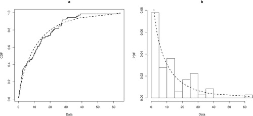
First, fit the P-EHRD to the data and compare its goodness-of-fit, using Kolmogorov-Smirnov (K-S) statistic, with its sub-models such as the linear hazard rate distribution (LHRD), the power hazard rate distribution (PHRD), and the exponential hazard rate distribution (EHRD). The ML estimates of the unknown parameters are obtained and then the values of K-S statistics and their corresponding p-values are calculated. The results are presented in Table 7. It is clear from Table 7 that the P-EHRD has the highest p-value of K-S test statistic and thus yields a better fit than LHRD, PHRD and EHRD. The empirical cdf versus fitted cdf and the histogram of the data versus fitted pdf for the P-EHRD are presented in Figure 1 which indicate the P-EHRD provides a good fit to the data.

Table 7. ML estimates of the parameters, K-S statistic, and corresponding p-value.

Distribution	$\widehat{a}$	$\widehat{b}$	$\widehat{c}$	$\widehat{k}$	K-S statistic	p-value
LHRD	$8.4\times {10}^{-13}$	0.0819	–	–	0.1422	0.1087
PHRD	0.0986	–	–	−0.0980	0.1055	0.3991
EHRD	–	0.0819	$5.9\times {10}^{-5}$	–	0.8102	0.0001
P-EHRD	0.1078	$1.5\times {10}^{-6}$	0.1784	−0.1560	0.0856	0.6657

Figure 1. (a) The empirical cdf (stair) versus fitted cdf (dotted curve). (b) Histogram of the data versus fitted pdf.

During this period, the following eight upper record values were observed under the random sampling scheme: $\underset{\sim }{r}:1.7,2.2,14.4,20.6,25.5,37.6,39.0,64.0.$

Based on these record data, the ML estimates of the parameters a, b, c and k, respectively from (10(10) $$a=g(b,c,k)=\frac{(k+1)\left(n-\frac{b}{c}(e^{c{r}_n}-1)\right)}{r_n^{k+1}}$$(10) ) to (13(13) $$\frac{\partial \ell }{\partial k}=\sum _{i=1}^n\frac{g(b,c,k)r_i^k\hspace{0.17em}\text{log}\hspace{0.17em}{r}_i}{g(b,c,k)r_i^k+b{e}^{c{r}_i}}-\frac{g(b,c,k)}{{(k+1)}^2}{r}_n^{k+1}\left[(k+1)\hspace{0.17em}\text{log}\hspace{0.17em}{r}_n-1\right]=0.$$(13) ) are obtained as $$\widehat{a}=0.3118,\hspace{1em}\widehat{b}=5.8\times {10}^{-7},\hspace{1em}\widehat{c}=0.1167,\hspace{1em}\mathrm{and}\hspace{1em}\widehat{k}=-0.3089$$ with the corresponding standard errors (Se), respectively as $$\mathit{Se}(\widehat{a})=0.2345,\hspace{1em}\mathit{Se}(\widehat{b})=8.9\times {10}^{-6},\hspace{1em}\mathit{Se}(\widehat{c})=0.0326,\hspace{1em}\mathrm{and}\hspace{1em}\mathit{Se}(\widehat{k})=0.2444.$$ Substituting the ML estimates of the unknown parameters in (15(15) $$\widehat{V}=\left(\begin{array}{cccc}{\widehat{V}}_{11}& {\widehat{V}}_{12}& {\widehat{V}}_{13}& {\widehat{V}}_{14}\\ {\widehat{V}}_{21}& {\widehat{V}}_{22}& {\widehat{V}}_{23}& {\widehat{V}}_{24}\\ {\widehat{V}}_{31}& {\widehat{V}}_{32}& {\widehat{V}}_{33}& {\widehat{V}}_{34}\\ {\widehat{V}}_{41}& {\widehat{V}}_{42}& {\widehat{V}}_{43}& {\widehat{V}}_{44}\end{array}\right)={\left(\begin{array}{cccc}{\widehat{I}}_{11}& {\widehat{I}}_{12}& {\widehat{I}}_{13}& {\widehat{I}}_{14}\\ {\widehat{I}}_{21}& {\widehat{I}}_{22}& {\widehat{I}}_{23}& {\widehat{I}}_{24}\\ {\widehat{I}}_{31}& {\widehat{I}}_{32}& {\widehat{I}}_{33}& {\widehat{I}}_{34}\\ {\widehat{I}}_{41}& {\widehat{I}}_{42}& {\widehat{I}}_{43}& {\widehat{I}}_{44}\end{array}\right)}^{-1},$$(15) ), the estimate of the variance-covariance matrix $\widehat{V}$ is obtained as $$\widehat{V}=\left(\begin{array}{cccc}0.0550& 5\times {10}^{-9}& -0.0013& -0.0506\\ 5\times {10}^{-9}& 8\times {10}^{-11}& -2\times {10}^{-6}& -2\times {10}^{-8}\\ -0.0013& -2\times {10}^{-6}& 0.0011& 0.0035\\ -0.0506& -2\times {10}^{-8}& 0.0035& 0.0597\end{array}\right).$$ The LS and Bayes estimates of the parameters a, b, c and k under SE and LINEX loss functions are obtained and the 95% asymptotic, Boot-p and Boot-t confidence intervals and the 95% HPD credible intervals of the parameters a, b, c, and k are computed. The predict value of the next record, $Y=r_{n+1},$ using the ML and Bayesian approaches is also computed. The Boot-p and Boot-t confidence intervals are obtained based on 1,000 bootstrap samples. To compute the Bayes estimates of the parameters a, b, c, and k, and the associated 95% HPD credible intervals, the hyperparameters as $({\alpha }_1,{\beta }_1)=({\alpha }_4,{\beta }_4)=(0.5,0.25)$ and $({\alpha }_2,{\beta }_2)=({\alpha }_3,{\beta }_3)=(1,0.05)$ to reflect little prior information are used. A total of N = 10,000 MCMC samples were generated and the first M = 2,000 values were discarded as burn-in period. Figure 2 shows the simulated values and Histogram of the parameters a, b, c, and k generated by Algorithm 2. All the point and interval estimates of the parameters are tabulated in Table 8.

Figure 2. Simulated values and histogram of the parameters a, b, c, and k.

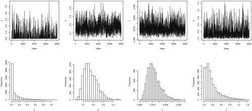
Table 8. The point and interval estimates of the parameters based on record flood values.

Parameters	a	b	c	k	Y
Methods			Point estimates
ML	0.3118	$5.8\times {10}^{-7}$	0.1167	−0.3089	79.8
LS	0.2899	$2.6\times {10}^{-8}$	0.2247	−0.5678	−
BS	0.0758	0.1888	0.0129	−0.4977	66.3
BL (d = 2)	0.0647	0.1855	0.0129	−0.6328	64.8
BL (d = −1)	0.0833	0.1905	0.0130	−0.3594	65.1
Methods			Interval estimates
AMLE	(−0.1478, 0.7716)	(−$1\times {10}^{-5},2\times {10}^{-5}$)	(0.0527, 0.1806)	(−0.7880, 0.1701)
Boot-p	(0.0087, 0.5597)	($2\times {10}^{-23},$ 0.0037)	(0.0117, 0.1504)	(−0.6145, 0.8806)
Boot-t	(0.1435, 0.5176)	(−$6\times {10}^{-7},$ 0.0110)	(0.0781, 0.2369)	(−1.6530, 0.5500)
MCMC	(0.0001,0.4109)	(0.0899,0.3148)	(0.0048,0.0246)	(−0.9736,0.6983)

7. Conclusions

In this paper, upper record samples from the P-EHRD are considered for estimating the unknown parameters and predicting the future record values. A Monte Carlo simulation study is conducted to examine and compare the performance of the proposed methods for parameters estimation and prediction of the future record values. The performances of the ML, LS and Bayes estimates under SE and LINEX loss functions are compared in terms of their ERs. The performances of the asymptotic, Boot-p and Boot-t confidence intervals and the HPD credible intervals are compared in terms of their coverage probability and expected length. The MSPEs are also used to compare the performances of the ML and Bayes point predictors. Based on simulation results, it was observed that the LS estimates perform better than the ML estimates in the estimation of parameters a and b, while the ML estimates perform better for the estimation of parameters c and k in most of the cases, especially when the sample size is large. The Bayes estimates under various loss functions show different performances in terms of their ERs. The performances of the Bayes estimates under SE loss function are better than the ML and LS estimates in most of the cases, except for estimation of b. The performances of the Bayes estimates under the LINEX loss function are dependent on the values of the shape parameter d and incomparable in general. Also, the Boot-p confidence intervals have better performances in comparison with the approximate confidence intervals and the Boot-t confidence intervals. The HPD credible intervals perform better than the approximate confidence intervals in most of the cases, except for estimation of b, but their performances are not preferable to the Boot-p confidence intervals in general. The point Bayes predictors were observed to perform better than the ML predictors in terms of MSPEs. Finally, an example of record flood values is used to illustrate the proposed methods of parameters estimation and prediction of the future record value.

Acknowledgments

The authors are grateful to the Editor, Associate Editor, and anonymous referees for making helpful comments and suggestions on an earlier version of this article which resulted in this improved version.

Appendix

The elements of the observed information matrix I are as follows: $$\begin{array}{c}{I}_{11}=-\frac{{\partial }^2\ell }{\partial a^2}=\sum _{i=1}^n\frac{r_i^{2k}}{{(a{r}_i^k+b{e}^{c{r}_i})}^2},\hspace{1em}{I}_{12}=-\frac{{\partial }^2\ell }{\partial a\partial b}=\sum _{i=1}^n\frac{r_i^k{e}^{c{r}_i}}{{(a{r}_i^k+b{e}^{c{r}_i})}^2},\\ I_{13}=-\frac{{\partial }^2\ell }{\partial a\partial c}=\sum _{i=1}^n\frac{b{r}_i^{k+1}{e}^{c{r}_i}}{{(a{r}_i^k+b{e}^{c{r}_i})}^2},\hspace{1em}{I}_{22}=-\frac{{\partial }^2\ell }{\partial b^2}=\sum _{i=1}^n\frac{e^{2c{r}_i}}{{(a{r}_i^k+b{e}^{c{r}_i})}^2},\\ I_{24}=-\frac{{\partial }^2\ell }{\partial b\partial k}=\sum _{i=1}^n\frac{a{r}_i^k\hspace{0.17em}\text{log}\hspace{0.17em}{r}_i{e}^{c{r}_i}}{{(a{r}_i^k+b{e}^{c{r}_i})}^2},\hspace{1em}{I}_{34}=-\frac{{\partial }^2\ell }{\partial c\partial k}=\sum _{i=1}^n\frac{\mathit{ab}{r}_i^{k+1}\hspace{0.17em}\text{log}\hspace{0.17em}{r}_i{e}^{c{r}_i}}{{(a{r}_i^k+b{e}^{c{r}_i})}^2},\\ I_{23}=-\frac{{\partial }^2\ell }{\partial b\partial c}=-\sum _{i=1}^n\frac{a{r}_i^{k+1}{e}^{c{r}_i}}{{(a{r}_i^k+b{e}^{c{r}_i})}^2}+\frac{1}{c^2}(c{r}_n{e}^{c{r}_n}-e^{c{r}_n}+1),\\ I_{33}=-\frac{{\partial }^2\ell }{\partial c^2}=-\sum _{i=1}^n\frac{\mathit{ab}{r}_i^{k+2}{e}^{c{r}_i}}{{(a{r}_i^k+b{e}^{c{r}_i})}^2}+\frac{b}{c^3}\left(e^{c{r}_n}{(c{r}_n-1)}^2+e^{c{r}_n}-2\right),\\ I_{14}=-\frac{{\partial }^2\ell }{\partial a\partial k}=-\sum _{i=1}^n\frac{b{r}_i^k\hspace{0.17em}\text{log}\hspace{0.17em}{r}_i{e}^{c{r}_i}}{{(a{r}_i^k+b{e}^{c{r}_i})}^2}+\frac{1}{{(k+1)}^2}{r}_n^{k+1}\left[(k+1)\hspace{0.17em}\text{log}\hspace{0.17em}{r}_n-1\right],\\ I_{44}=-\frac{{\partial }^2\ell }{\partial k^2}=-\sum _{i=1}^n\frac{\mathit{ab}{r}_i^k{\hspace{0.17em}\text{log}\hspace{0.17em}}^2{r}_i{e}^{c{r}_i}}{{(a{r}_i^k+b{e}^{c{r}_i})}^2}+\frac{a}{{(k+1)}^3}{r}_n^{k+1}\left[{\left((k+1)\hspace{0.17em}\text{log}\hspace{0.17em}{r}_n-1\right)}^2+1\right].\end{array}$$

References

- Ahsanullah, M. (2004). Record values: Theory and applications. Lanham, MD: University Press of America Inc.
- Arnold, B. C., Balakrishnan, N., & Nagaraja, H. N. (1998). Records. New York: John Wiley and Sons.
- Asgharzadeh, A., & Fallah, A. (2011). Estimation and prediction for exponentiated family of distributions based on records. Communications in Statistics - Theory and Methods, 40(1), 68–83. doi:10.1080/03610920903350564
- Asgharzadeh, A., Fallah, A., Raqab, M. Z., & Valiollahi, R. (2018). Statistical inference based on Lindley record data. Statistical Papers, 59(2), 759–779. doi:10.1007/s00362-016-0788-1
- Bain, L. (1974). Analysis for the linear failure-rate life testing distribution. Technometrics, 15, 551–559. doi:10.1080/00401706.1974.10489237
- Basak, P., & Balakrishnan, N. (2003). Maximum likelihood prediction of future record statistic. Mathematical and statistical methods in reliability. In Series on quality, reliability and engineering statistics (pp. 159–175), Eds. Lindquist, B. H. and Doksum, K. A., vol 7. Singapore: World Scientific Publishing.
- Chandler, K. N. (1952). The distribution and frequency of record values. Journal of the Royal Statistical Society: Series B (Methodological), 14, 220–228. doi:10.1111/j.2517-6161.1952.tb00115.x
- Chen, M. H., & Shao, Q. M. (1999). Monte Carlo estimation of Bayesian credible and HPD intervals. Journal of Computational and Graphical Statistics, 8, 69–92. doi:10.1080/10618600.1999.10474802
- Choulakian, V., & Stephens, M. A. (2001). Goodness-of-fit for the generalized Pareto distribution. Technometrics, 43(4), 478–484. doi:10.1198/00401700152672573
- Dey, S., Dey, T., Salehi, M., & Ahmadi, J. (2013). Bayesian inference of generalized exponential distribution based on lower record values. American Journal of Mathematical and Management Sciences, 32, 1–18.
- Efron, B. (1982). The jackknife, the bootstrap and other re-sampling plans. CBMS-NSF regional conference series in applied mathematics (No. 38). Philadelphia, PA: SIAM.
- Efron, B., & Tibshirani, R. J. (1993). An introduction to the bootstrap. New York: Chapman and Hall.
- Gelfand, A. E., & Smith, A. F. M. (1990). Sampling-based approaches to calculating marginal densities. Journal of the American Statistical Association, 85(410), 398–409. doi:10.1080/01621459.1990.10476213
- Gompertz, B. (1825). On the nature of the function expressive of the law of human mortality, and on a new mode of determining the value of life contingencies. Philosophical Transaction of the Royal Society of London, 115, 513–583.
- Hall, P. (1988). Theoretical comparison of bootstrap confidence intervals. The Annals of Statistics, 16(3), 927–953. doi:10.1214/aos/1176350933
- Krishna, H., & Kumar, K. (2013). Reliability estimation in generalized inverted exponential distribution with progressively type II censored sample. Journal of Statistical Computation and Simulation, 83(6), 1007–1024. doi:10.1080/00949655.2011.647027
- Kumar, D., Kumar, M., Saran, J., & Jain, N. (2017). The Kumaraswamy-Burr III distribution based on upper record values. American Journal of Mathematical and Management Sciences, 36(3), 205–228. doi:10.1080/01966324.2017.1318099
- Lin, C. T., Wu, S. J. S., & Balakrishnan, N. (2003). Parameter estimation for the linear hazard rate distribution based on records and inter-record times. Communications in Statistics - Theory and Methods, 32(4), 729–748. doi:10.1081/STA-120018826
- Miller, R. G. (1981). Survival analysis. New York: John Wiley.
- Mugdadi, A. R. (2005). The least squares type estimation of the parameters in the power hazard function. Applied Mathematics and Computation, 169(2), 737–748. doi:10.1016/j.amc.2004.09.064
- Pak, A., & Dey, S. (2019). Statistical inference for the power Lindley model based on record values and inter-record times. Journal of Computational and Applied Mathematics, 347, 156–172. doi:10.1016/j.cam.2018.08.012
- Raqab, M. Z., Bdair, O. M., & Al-Aboud, F. M. (2018). Inference for the two-parameter bathtub-shaped distribution based on record data. Metrika, 81(3), 229–253. doi:10.1007/s00184-017-0641-0
- Soliman, A. A., Abd Ellah, A. H., & Sultan, K. S. (2006). Comparison of estimates using record statistics from Weibull model: Bayesian and non-Bayesian approaches. Computational Statistics & Data Analysis, 51(3), 2065–2077. doi:10.1016/j.csda.2005.12.020
- Swain, J., Venkatraman, S., & Wilson, J. (1988). Least squares estimation of distribution function in Johnson’s translation system. Journal of Statistical Computation and Simulation, 29(4), 271–297. doi:10.1080/00949658808811068
- Tarvirdizade, B., & Nematollahi, N. (2019). A new flexible hazard rate distribution: Application and estimation of its parameters. Communications in Statistics - Simulation and Computation, 48(3), 882–899. doi:10.1080/03610918.2017.1402039
- Tierney, L. (1994). Markov chains for exploring posterior distributions. The Annals of Statistics, 22(4), 1701–1728. doi:10.1214/aos/1176325750
- Varian, H. (1975). A Bayesian approach to real estate assessment. In Studies in Bayesian econometrics and statistics in honor of Leonard J. Savege (pp. 195–208). Amsterdam, The Netherlands: North Holland.