A new discrete distribution

Abstract

A new one-parameter discrete distribution is introduced. Its mathematical properties and estimation procedures are derived. Four real data sets are used to show that the new model performs at least as well as the traditional one-parameter discrete models and other newly proposed two-parameter discrete models.

• discrete gamma
• discrete Lindley
• discrete Weibull

1. Introduction

The traditional discrete distributions (geometric, Poisson, etc.) have limited applicability as models for reliability, failure times, counts, etc. This has led to the development of some discrete distributions based on popular continuous models for reliability, failure times, etc. Of these, the most popular is the discrete Weibull distribution.

The discrete Weibull distribution was introduced by Nakagawa and Osaki [1], Stein and Dattero [2], Khan et al. [3] and Kulasekera [4]. It has since received widespread applications. The probability mass function of the discrete Weibull distribution is

for x=0, 1, 2, … , where 0<q<1 and β>0. Note that Equation (1) has two parameters. A particular case of Equation (1) for β=2, the discrete Rayleigh distribution, has been studied by Roy [5,6].

Some application areas of the discrete Weibull distribution have been testing contagion in the context of renewal theory [7]; pacemaker/accumulator process in animal timing [8]; warranty cost on optimization of the economic manufacturing quality [9]; estimation of replicative senescence via population dynamics models [10]; stress–strength reliability [5]; evaluation of reliability of complex systems [11]; duration-based backtesting of value at risk [12]; tree recruitment [13]; software reliability growth modelling [14–17]; opportunity-based age replacement policy [18]; wafer probe operation in semiconductor manufacturing [19,23]; inventory models with imperfect production processes [20]; off-line inspection with rework consideration [21,22]; customer-base valuation [24]; failure-counts-based health evaluation of a bus fleet [25]; construction of annual fire risk maps [26]; minimal availability variation design of repairable systems [27,28]; undulation analysis of instantaneous availability [27,28] and microbial counts in water [29].

Among other newly developed distributions corresponding to continuous analogues, only the discrete gamma appears to have received significant applications. It appears to have been used first by Yang \cite[Equations (8)–(12)]{30} in the area of molecular biology and evolution. The probability mass function of the discrete gamma distribution is

for x=0, 1, 2, … , where α>0, β>0, is the incomplete gamma function and is the gamma function. Note again that Equation (2) has two parameters.

Since Yang [30], many researchers in molecular biology and evolution have used the discrete gamma distribution (see, e.g. [31–34] for recent references).

The most recent discrete distributions are those due to Krishna and Pundir [35], Aghababaei Jazi et al. [36] and Gómez-Déniz [37]. Krishna and Pundir [35] construct discrete analogues of the continuous Burr and Pareto distributions. Aghababaei Jazi et al. [36] construct a discrete analogue of the continuous inverse Weibull distribution. Gómez-Déniz [37] constructs a discrete analogue of the generalized exponential distribution due to Marshall and Olkin [38]. Being the most recent, these three distributions have not yet received any applications. All three distributions have at least two parameters each. All three distributions have moments expressed in terms of either infinite sums or non-standard special functions. Besides, data analysis shows that the distribution due to Aghababaei Jazi et al. [36] produces fits similar to the discrete Weibull distribution given by Equation (1). Therefore, we shall not discuss these distributions in subsequent sections.

The aim of this paper is to introduce a new one-parameter discrete distribution. This model is shown to perform at least as well as the traditional models (geometric and Poisson) and the newly developed models (discrete Weibull and discrete gamma) with respect to four real data sets on failure times and counts. Two of the data sets consists of failure times. The other two data sets consists of counts. Not many of the known discrete distributions can provide accurate models for both times and counts. For example, the Poisson distribution is used to model counts but not times. It is remarkable that the proposed discrete distribution provides the best fit for both times and counts in spite of having only one parameter. Potential application areas of the new distribution could include those mentioned above and many more.

The binomial and negative binomial distributions are not considered because they are not considered to be popular models for reliability, failure times, counts, etc. This is partly because they are not defined over the set of all non-negative integers. Also, the negative binomial distribution does not share the ‘time-to-event’ interpretation that the geometric distribution has. Besides, the binomial and negative binomial distributions can be approximated well by the Poisson distribution under suitable conditions.

The new distribution is specified by the probability mass function:

where , for θ>0, and x=0, 1, 2, … . The corresponding cumulative distribution function and survival function are

and

respectively, for x=0, 1, 2, … . This survival function is the discrete version of that corresponding to the continuous Lindley distribution [39]. Therefore, we may refer to the distribution given by Equation (3) as the discrete Lindley distribution. The geometric distribution is contained as a particular case of Equation (3) as .

We shall see later that the parameter θ can be interpreted as a strict upper bound on the failure rate function, an important characteristic for lifetime models, corresponding to Equations (3)–(5). Not many discrete distributions have their parameters directly interpretable in terms of their failure rate functions. One exception is the geometric distribution, but in this case the failure rate function is a constant.

We shall also see later that the discrete Lindley distribution always allows for increasing failure rates. It does not allow for a constant or a decreasing failure rate. The geometric, discrete Weibull and the discrete gamma distributions do allow for constant and decreasing failure rates. These are very unrealistic features because there are hardly any real-life systems that have constant or decreasing failure rates.

Another interpretation of the discrete Lindley distribution can be seen in terms of its mean residual lifetime. It is not difficult to see from Equation (5) that

and

The second term in Equation (6), that is, the infinite series term, and the second term in Equation (7) can be thought of as corrections for the ‘memory less property’ of the geometric distribution. If the waiting time is small, then the expected excess time is large. On the other hand, if the waiting time is large then the expected excess time is small. Therefore, the correction term is reasonable.

Another attractive feature of the discrete Lindley distribution is that it has closed-form expressions for its cumulative distribution function and failure rate function. This is not the case for the Poisson or discrete gamma distributions.

The contents of this paper are organized as follows. The mathematical properties of the new distribution given by Equation (3) are derived in Section 2. The derived properties include shape of the probability mass function, failure rate function and its shape, quantile function, median, probability generating function, moment generating function, characteristic function, moments, conditional moments, factorial moments, cumulants, variance, coefficient of variation, skewness, kurtosis, stochastic orderings, distribution of order statistics, moments of order statistics, asymptotic distribution of the extreme order statistics, L moments, distribution of range, Shannon entropy, Rényi entropy, cumulative residual entropy, mean deviation about the mean, mean deviation about the median, Bonferroni curve, Lorenz curve, distribution of the sum of random variables, distribution of the difference of random variables, distribution of the maximum of random variables, distribution of the minimum of random variables, and reliability measure. The estimation procedures for the method of moments, method of maximum likelihood and the method of maximum likelihood incorporating censoring are derived in Section 3. An application involving four real data sets is discussed in Section 4.

2. Mathematical properties

Here, we derive various mathematical properties of the discrete Lindley distribution. The properties derived include shape properties (Section 2.1), quantile function (Section 2.2), moment properties (Section 2.3), stochastic orderings (Section 2.4), order statistics (Section 2.5), asymptotic distribution of extreme order statistics (Section 2.6), L moments (Section 2.7), distribution of range (Section 2.8), entropies (Section 2.9), mean deviations (Section 2.10), Bonferroni and Lorenz curves (Section 2.11), distribution of sums and differences (Section 2.12), distribution of maximums and minimums (Section 2.13), and reliability measure (Section 2.14).

2.1 Shape properties

Theorem 2.1

The discrete Lindley distribution is unimodal.

Proof The probability mass function (Equation (3)) satisfies the log-concave inequality for x=0, 1, 2, … . Therefore, the result follows using Theorem 3 of [40].

It follows from Theorem 2.1 that the discrete Lindley distribution is unimodal and has a discrete increasing failure rate.

Theorem 2.2

The mode of the discrete Lindley distribution is where [z] is the integer part of z and ℤ is the set of integers.

Proof Since the discrete Lindley distribution is unimodal, its probability mass function satisfies the following inequalities: and where x₀ is the mode of p(x). Therefore, and This completes the proof.

It follows from Equations (3) and (5) that the failure rate of the discrete Lindley distribution is

This function is concave and increasing in x=0, 1, … implying again that the discrete Lindley distribution has a discrete increasing failure rate. Note that Also, p (x)=0 and . If θ is small then R (∞) is approximately equal to θ. Therefore, R(x) is bounded above by θ for all x.

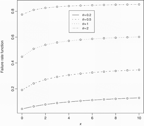
Figure 1 shows some possible shapes of Equation (3). We can see that the probability mass function is always unimodal. If θ≥1, the mode is at zero. For θ<1, the mode is positive. Figure 2 shows some possible shapes of Equation (8). We can see that the failure rate is increasing with respect to both x and θ.

Figure 1. Probability mass function of the discrete Lindley distribution for θ=0.2, 0.5, 1, 2.

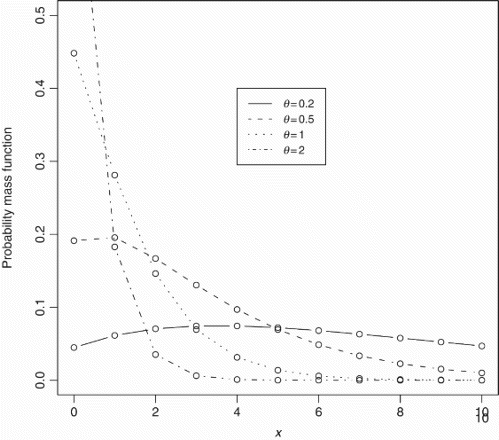
Figure 2. Failure rate function of the discrete Lindley distribution for θ=0.2, 0.5, 1, 2.

2.2 Quantile function

The quantile function of the discrete Lindley distribution, say Q (u), defined by F (Q (u))=u is the root of the equation

for 0<u<1. Substituting , one can rewrite Equation (9) as for 0<u<1. Therefore, the solution for Z (u) is

for 0<u<1, where W (·) is the Lambert W function due to Lambert [41]. See [42] for detailed properties of the Lambert W function. Inverting Equation (10), one obtains

for 0<u<1, where denotes floor. In particular, the median of the discrete Lindley distribution is

A series expansion for Equation (11) around u=1 can be obtained as

where . However, these expansions may not be needed as in-built routines for computing W (·) which are widely available, for example, {\sf ProductLog[·]} in Mathematica.

2.3 Moment properties

Let X be a discrete Lindley random variable. Then, the probability generating function of X can be expressed as

The corresponding moment generating function is The corresponding characteristic function is where .

Theorem 2.3

Let denote the kth-order moment. Let denote the kth-order descending factorial moment. Let denote the kth-order conditional moment. Let κ_k denote the kth-order cumulant. Then, μ_k, μ_(k), c_k and κ_k for the discrete Lindley distribution are

and

for k=1, 2, … , where

Proof For Equation (15), write and apply Equation (0.232.3) in [43] to calculate the infinite sums. For Equation (16), differentiate G(s), given by Equation (14), k times and evaluate at s=1. For Equation (17), use Equation (6) to write and apply Equation (0.232.3) in [43] to calculate the infinite sums. For Equation (18), using the series expansions for log (1+z) and exp (z), we can express The result follows.

The first four moments of the discrete Lindley distribution are The corresponding variance, coefficient of variation, skewness and kurtosis are The first four conditional moments of the discrete Lindley distribution are The corresponding conditional variance, conditional coefficient of variation, conditional skewness and conditional kurtosis are and

2.4 Stochastic orderings

Stochastic ordering is an important measure to judge comparative behaviours of random variables. Many stochastic orders exist and have various applications (see [44] for details). Theorems 2.4–2.6 and Corollaries 2.1–2.2 give some results on stochastic orderings of the discrete Lindley distribution. The orders considered here are the likelihood ratio order ≤_lr, the stochastic order ≤_st, the hazard rate order ≤_hr, the reversed hazard rate order ≤_rh and the expectation order ≤_E.

Theorem 2.4

Let X be a random variable with probability mass function, p_X (·), given by Equation (3). Let Y be a geometric random variable with the probability mass function x=0, 1, 2, … . Then, and is an increasing function in x.

Proof Since we have for all θ>0 and p∈(0, 1). The proof is complete.

Corollary 2.1 follows from noting that implies , , and consequently Y≤_EX.

Corollary 2.1

From Theorem 2.4, we obtain

• (i)  that is, for all x.

• (ii)  that is, for all x.

• (iii)  that is, for all x.

• (iv) Y≤_EX, that is, .

Theorem 2.5

Let X₁ and X₂ be discrete Lindley random variables with parameters and respectively. Then, if and only if p₂≤p₁.

Proof We have if and only if for all x if and only if for all x if and only if p₂≤p₁. The proof is complete.

By a similar argument, we can show the following.

Theorem 2.6

Let X₁ and X₂ be discrete Lindley random variables with parameters (θ₁, p) and (θ₂, p), respectively. Then, if and only if .

Corollary 2.2 follows from Theorems 2.5 and 2.6.

Corollary 2.2

If X₁ and X₂ are discrete Lindley random variables with parameters and respectively, with p₂≤p₁, then .

If X₁ and X₂ are discrete Lindley random variables with parameters (θ₁, p) and (θ₂, p), respectively, with then .

2.5 Order statistics

Let be a random sample from Equation (3). Let denote the corresponding order statistics. Then, the probability mass function and the cumulative distribution function of the ith-order statistic, X_i:n, are given by and respectively, where F(·) is given by Equation (4). The kth-order moment of X_i:n can be expressed as

where the final step follows by Equation (0.232.3) in [43] and S (a, b) is given by Equation (19).

2.6 Asymptotic distribution of extreme order statistics

Sometimes it is of interest to consider the asymptotic distributions of the extreme order statistics, that is, X_{1: n} and X_{n: n}. It can be seen that It can also be seen that Hence, it follows from Theorem 1.6.2 in [45] that there must be norming constants a_n>0, b_n, c_n>0 and d_n such that and as . The form of the norming constants can also be determined. For instance, using Corollary 1.6.3 in [45], one can see that and a_n=θ, where F⁻¹ (·) denotes the inverse function of F (·). By Equation (13), as n→∞.

2.7 L moments

L moments are summary statistics for probability distributions and data samples [46]. They are analogous to ordinary moments but are computed from linear functions of the ordered data values. The kth L moment is defined by where . In particular, , , and . In general, , so it can be computed using Equation (20). The L moments have several advantages over ordinary moments: for example, they apply for any distribution having finite mean and no higher order moments need to be finite.

2.8 Distribution of range

From [47], we obtain for y=0, 1, … . If denotes the range of the order statistics, then

2.9 Entropies

An entropy is a measure of variation of the uncertainty. Three most popular entropies are Shannon entropy [48], Rényi [49] entropy, and the cumulative residual entropy [50]. We now derive expression for these entropies when X is a discrete Lindley random variable.

The Shannon entropy [48] is defined by . Using the Taylor series expansion for log (1+z), we obtain where μ_k are given by Equation (15).

Rényi entropy [49] is defined by where γ>0 and γ≠1. For the probability mass function given by Equation (3), where the final step follows by Equation (0.232.3) in [43], S (a, b) is given by Equation (19) and .

The cumulative residual entropy [50] is defined by

Using the Taylor series expansion for log (1+z), we obtain where μ_k are given by Equation (15).

2.10 Mean deviations

The amount of scatter in a population is evidently measured to some extent by the totality of deviations from the mean and median. These are known as the mean deviation about the mean and the mean deviation about the median – defined by and respectively, where μ=E (X) and denotes the median. The measures, δ₁ (X) and δ₂ (X), can be calculated using the relationships and respectively.

Let X be an independent discrete Lindley random variable with parameter θ. Also, let and let Then, where the final step follows by Equations (0.113) and (0.114) in [43]. It follows that and

2.11 Bonferroni and Lorenz curves

The Bonferroni and Lorenz curves for a non-negative random variable X are defined as the graphs of the ratios

and

respectively, against F(x). The Lorenz curve has the properties L(p)≤p, L (0)=0 and L (1)=1. If X represents annual income, L(p) is the proportion of total income that accrues to individuals having the 100 p% lowest incomes. If all individuals earn the same income, then L(p)=p for all p. The area between the line L(p)=p and the Lorenz curve may be regarded as a measure of inequality of income, or more generally, of variability of X (see [51,52] for extensive discussion of Lorenz curves). A similar interpretation applies to the Bonferroni curve.

Let X be an independent discrete Lindley random variable with parameter θ. Also, let , u=F (x) and μ=E (X). Then, Equations (21) and (22) can be expressed as and respectively, for 0<u<1. The Bonferroni curve is a graph of B (u) versus u. The Lorenz curve is a graph of L (u) versus u.

2.12 Distribution of sums and differences

Sums and differences of random variables arise in reliability. Let X and Y be independent discrete Lindley random variables with parameters θ₁ and θ₂, respectively. Also, let and . Then, the probability mass function of the sum, S=X+Y, can be expressed as

where the final step follows by Equations (0.112)–(0.114) in [43]. Similar calculations show that the corresponding cumulative distribution function is

In the particular case (with p₁=p₂=p), Equations (23) and (24) reduce to the simpler forms and respectively.

The probability mass function of the difference, D=X−Y, can be expressed as

where the final step follows by Equation (0.232.3) in [43] and S (a, b) is given by Equation (19). Similar calculations show that the corresponding cumulative distribution function is

where S (a, b) is given by Equation (19). In the particular case (with p₁=p₂=p), Equations (25) and (26) reduce to the simpler forms and respectively, where S (a, b) is given by Equation (19).

The moments of S=X+Y and D=X−Y can be calculated using the facts that and respectively.

2.13 Distribution of maximums and minimums

Maximums and minimums of random variables also arise in reliability. Let X_i, i=1, 2, … , n, be independent discrete Lindley random variables with parameters θ_i, i=1, 2, … , n. Also, let for i=1, 2, … , n. Then, the cumulative distribution function of the minimum, , is

The cumulative distribution function of the maximum, , is

The moments of and can be calculated as and respectively, where S (a, b) is given by Equation (19).

2.14 Reliability measure

In the context of reliability, the stress–strength model describes the life of a component which has a random strength Y that is subjected to a random stress X. The component fails at the instant when the stress applied to it exceeds the strength, and the component will function satisfactorily whenever Y>X. Therefore, R=⪻(X<Y) is a measure of component reliability. It has many applications especially in engineering concepts such as structures, deterioration of rocket motors, static fatigue of ceramic components, fatigue failure of aircraft structures, and the ageing of concrete pressure vessels.

Suppose X and Y are independent discrete Lindley random variables with parameters θ₁ and θ₂, respectively. Let and . We can express R=⪻(X<Y) as where the final step follows by Equation (0.232.3) in [43] and S (a, b) is given by Equation (19).

3. Estimation

In this section, we estimate the unknown parameters of the discrete Lindley distribution using the methods of moments and maximum likelihood. We suppose that we have a random sample from Equation (3).

3.1 Moments estimation

For moments estimation, let m₁=(1/ denote the sample mean. Equating this with the theoretical mean given by Equation (16), we obtain

where . The method of moments estimator of θ is the root of this equation. The root can be found analytically if θ is small. Setting , we obtain The valid root of this quadratic equation is

A better approximation is to set . This gives the cubic equations:

or

The roots of Equations (31) and (32) can be obtained using the fact that the cubic equation has the roots

where . The values given by Equations (30) and (33)–(35) can be used as initial values for solving Equations (29) and for other estimation methods.

3.2 Maximum-likelihood estimation

Now consider estimation by the method of maximum likelihood. The log-likelihood function of θ is It follows that the maximum-likelihood estimator, θˆ, of θ is the root of the equation

The root can be found analytically if θ is small. Setting , we obtain The valid root of this quadratic equation is

A better approximation is to set . This gives the quadratic equation We can take θˆ to be the valid roots of one of

where An even better approximation is to set . This gives the cubic equation The roots of this equation are given by Equations (33)–(35). The values given by Equations (37), (38) and (33)–(35) can be used as initial values for solving Equation (36) and for other estimation methods.

For interval estimation of θ and tests of hypothesis, we require Fisher's information . It is given by where ,

and

The expectations, Equations (39) and (40), can be expressed as

and

where , and , where S (a, b) is given by Equation (19). Under regularity conditions, the asymptotic distribution of as is normal with zero mean and variance 1/I(θ).

A normal approximation is to assume that θˆ has a normal distribution with mean θ and variance . This approximation can be used to construct confidence intervals for θ and to test hypothesis of the kind . A confidence interval for θ is where I_1ˆ and I_2ˆ are given by Equations (41) and (42), respectively, with θ replaced by θˆ, and z_α/2 is the percentile of a standard normal variate. A likelihood ratio test of versus with significance level α is to reject H₀ if where c is such that .

It is reasonable to ask: how large should n be for the normal approximation to hold? This question is answered in the next section.

3.3 A simulation study

Here, we assess the performance of the maximum-likelihood estimate given by Equation (36) with respect to sample size n. The assessment is based on a simulation study:

• (1)  generate 10,000 samples of size n from Equation (3). The inversion method is used to generate samples, that is, variates of the discrete Lindley distribution are generated using where U∼ U(0, 1) is a uniform variate on the unit interval;

• (2)  compute the maximum-likelihood estimates for the 10,000 samples, say for i=1, 2, … , 10000.

• (3)  compute the biases and mean-squared errors given by and

We repeat these steps for with , hence computing bias (n) and MSE (n) for .

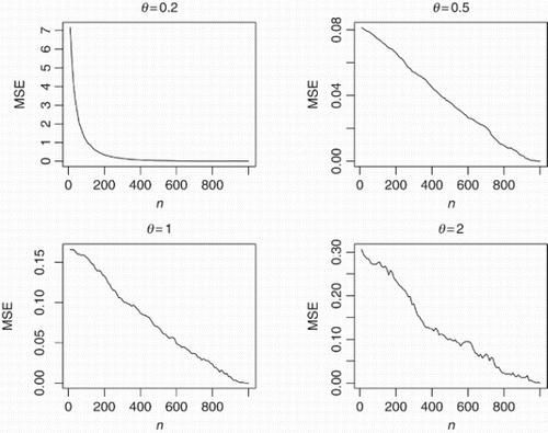
Figures 3 and 4 show how the biases and the mean-squared errors vary with respect to n. The broken line in Figure 3 corresponds to the biases being zero. The following observations can be made:

Figure 3. Bias(n) versus n=10, 20, … , 1000 for θ=0.2, 0.5, 1, 2.

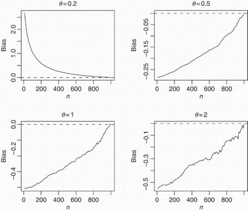
Figure 4. MSE(n) versus n=10, 20, … , 1000 for θ=0.2, 0.5, 1, 2.

• (1) the biases are positive for θ=0.2,

• (2) the biases are negative for θ=0.5, 1, 2,

• (3) the magnitude of bias always decreases to zero as n→∞,

• (4) the rate of decay of the magnitude appears approximately linear for θ=0.5, 1, 2,

• (5) the rate of decay for θ=0.2 appears much sharper,

• (6) the biases appear largest for θ=0.2,

• (7) the biases appear smallest for θ=0.5,

• (8) the mean-squared errors always decrease to zero as n→∞,

• (9) the rate of decrease appears approximately linear for θ=0.5, 1, 2,

• (10) the rate of decrease for θ=0.2 appears much sharper,

• (11) the mean-squared errors appear largest for θ=0.2,

• (12) the mean-squared errors appear smallest for θ=0.5.

We have presented results only for for reasons of space. But the results are similar for other choices for θ.

3.4 Censored maximum-likelihood estimation

Often with lifetime data, one encounters censoring. There are different forms of censoring: type I censoring, type II censoring, etc. Here, we consider the general case of multicensored data: there are n subjects of which

• n₀ are known to have the values ;

• n₁ are known to belong to the interval (S_i−1, S_i , ;

• n₂ are known to have exceeded R_i, i=1, … , n₂, but not observed any longer.

Note that . Note too that type I censoring and type II censoring are contained as particular cases of multicensoring.

In the case of multicensoring, the log-likelihood function is It follows that the maximum-likelihood estimator, θˆ, of θ is the root of the equation where . The corresponding information, I (θ), is too complicated to be presented here.

4. Data application

Here, we illustrate the superiority of the discrete Lindley distribution over the traditional models (geometric and Poisson) as well as the newly developed models (discrete Weibull and discrete gamma).

We use four real data sets. The first data set given in Table 1 consists of survival times in days of 72 guinea pigs. These data are taken from Table 6 in [53]. The data have been analysed by many authors, too many to cite here. Three of the most recent papers analysing the data are those by Alshunnar et al. [54], Kundu and Howlader [55] and Ghitany et al. [56]. These papers use continuous models to fit the data. The data are discrete by definition. Some summary statistics of the data are: minimum is 12, first quartile is 54.75, median 70, mean is 99.82, third quartile is 112.80, maximum is 376 and variance is 6580.122.

Table 1  Data set 1.

12 15 22 24 24 32 32 33 34 38 38 43 44 48

52 53 54 54 55 56 57 58 58 59 60 60 60 60

61 62 63 65 65 67 68 70 70 72 73 75 76 76

81 83 84 85 87 91 95 96 98 99 109 110 121

127 129 131 143 146 146 175 175 211 233 258 258

263 297 341 341 376

The second data set given in Table 2 consists of remission times in weeks for 20 leukaemia patients randomly assigned to a certain treatment. It is taken from page 346 of Lawless [57,58]. The data have been analysed recently by Damien and Walker [59] and Kottas [60]. Some summary statistics of this data are: minimum is 1, first quartile is 7, median is 16.5, mean is 19.55, third quartile is 28.25, maximum is 49 and variance is 216.05.

Table 2  Data set 2.

1 3 3 6 7 7 10 12 14 15 18 19

22 26 28 29 34 40 48 49

The third data set shown in Table 3 are the numbers of fires in Greece for the period from 1 July 1998 to 31 August of the same year [61]. Only fires in forest districts are considered. The sample size of these data are 123. Some summary statistics are: minimum is 0, first quartile is 2, median is 4, mean is 5.398, third quartile is 8, maximum 43 and variance is 30.0449.

Table 3  Data set 3.

2 4 4 3 3 1 2 4 3 1 1 0 5 5 0 3 1 1 0 1 0 2 0 1 2 0 0 0 0 0 0 0 0 0 1 4 2 2

1 2 1 2 0 2 2 1 0 3 2 1 2 2 7 3 5 2 5

4 5 6 5 4 3 8 43 8 4 4 3 10 5 4 5 12 3 8

12 10 11 6 1 8 9 12 9 4 8 12 11 8 6 4 7 9 15

12 15 15 12 9 16 7 11 9 11 6 5 20 9 8 8 5 7 10

6 6 5 5 15 6 8 5 6

The fourth data set given in Table 4 consists of the 2003 final examination marks of 48 slow space students in mathematics in the Indian Institute of Technology at Kanpur. The data set is taken from [62]. Some summary statistics of these data are: minimum is 4, first quartile is 14, median is 19.5, mean is 25.9, third quartile is 34, maximum is 86 and variance is 346.1379.

Table 4  Data set 4.

29 25 50 15 13 27 15 18 7 7 8 19 12 18 5 21 15 86 21 15 14 39 15 14

70 44 6 23 58 19 50 23 11 6 34 18 28 34 12 37 4 60 20 23 40 65 19 31

The five models (discrete Lindley, geometric, Poisson, discrete Weibull and discrete gamma) were fitted to each of the data sets by the method of moments. The parameter estimates, p-values and the Kolmogorov–Smirnov statistics are shown in Tables 4–8. The corresponding probability–probability plots are shown in Figures 5–8. The corresponding quantile–quantile plots are shown in Figures 9–12. The corresponding distribution plots comparing the fitted and observed distribution functions are shown in Figures 13–16.

Figure 5. Probability–probability plot for data set 1.

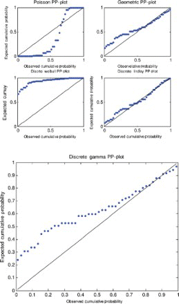
Figure 6. Probability–probability plot for data set 2.

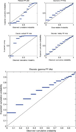
Figure 7. Probability–probability plot for data set 3.

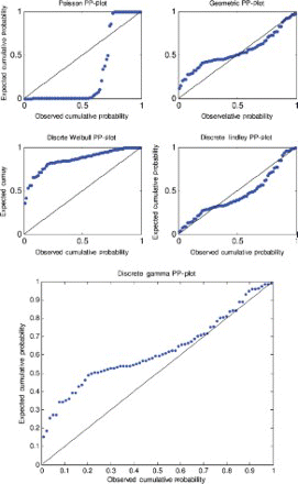
Figure 8. Probability–probability plot for data set 4.

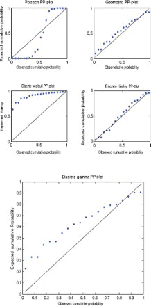
Figure 9. Quantile–quantile plot for data set 1.

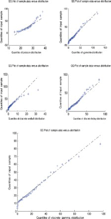
Figure 10. Quantile–quantile plot for data set 2.

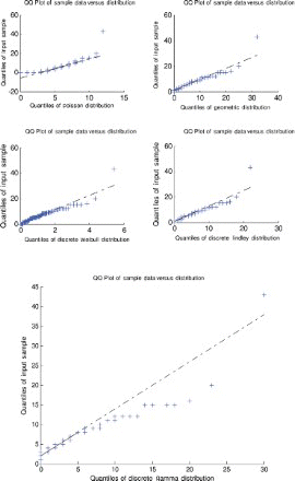
Figure 11. Quantile–quantile plot for data set 3.

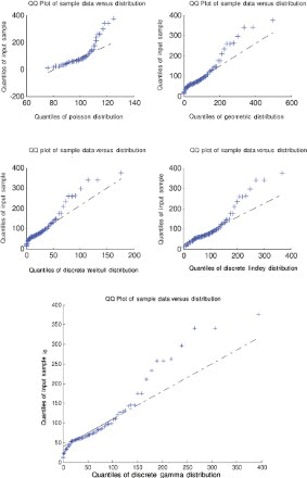
Figure 12. Quantile–quantile plot for data set 4.

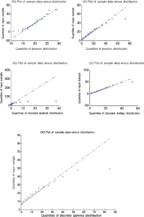
Figure 13. Distribution plots for data set 1.

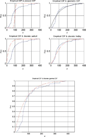
Figure 14. Distribution plots for data set 2.

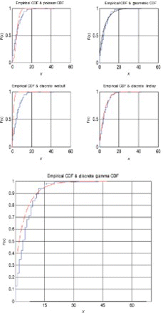
Figure 15. Distribution plots for data set 3.

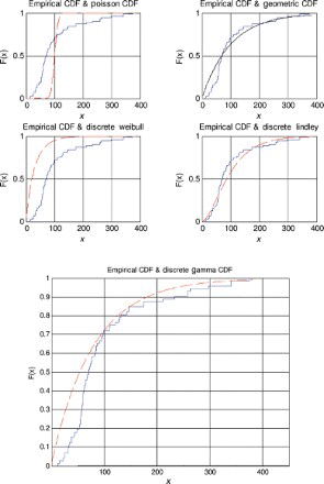
Figure 16. Distribution plots for data set 4.

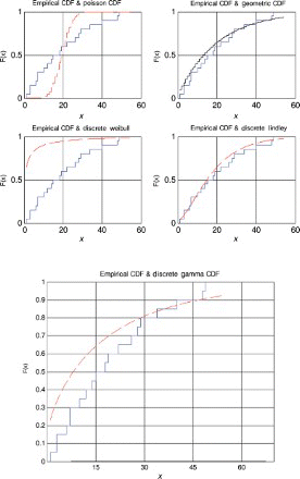
Table 5  Fitted estimates for data set 1.

Model	p(x)	Parameter estimates	p-Value	K–S statistic
Discrete Lindley	(3)	,	0.0683	0.1507
Poisson			9.5313	0.5755
Geometric			0.0020	0.2160
Discrete Weibull	(1)	,	1.0821	0.6140
Discrete gamma	(2)	,	4.1283 ×10^−6	0.2966

Note: K–S, Kolmogorov–Smirnov.

Table 6  Fitted estimates for data set 2.

Model	p(x)	Parameter estimates	p-Value	K–S statistic
Discrete Lindley	(3)	,	0.0541	0.2909
Poisson			0.0100	0.3523
Geometric			0.7436	0.1447
Discrete Weibull	(1)	,	3.5869	0.7233
Discrete gamma	(2)	,	0.0541	0.2909

Note: K–S, Kolmogorov–Smirnov.

Table 7  Fitted estimates for data set 3.

Model	p(x)	Parameter estimates	p-Value	K–S statistic
Discrete Lindley	(3)	,	0.0842	0.1122
Poisson			1.6048 ×10^−7	0.2547
Geometric			0.0024	0.1636
Discrete Weibull	(1)	,	2.7128	0.7642
Discrete gamma	(2)	,	2.8224 ×10^−8	0.2683

Note: K–S, Kolmogorov–Smirnov.

Table 8  Fitted estimates for data set 4.

Model	p(x)	Parameter estimates	p-Value	K–S statistic
Discrete Lindley	(3)	,	0.4677	0.1191
Poisson			2.4013 ×10^−7	0.3998
Geometric			0.0145	0.2223
Discrete Weibull	(1)	,	2.9221	0.7419
Discrete gamma	(2)	,	2.6082 ×10^−4	0.2993

Note: K–S, Kolmogorov–Smirnov.

A probability–probability plot is a plot of the observed probabilities against probabilities predicted by the fitted model. For example, for the discrete Lindley distribution, , j=1, 2, … , n, are plotted versus , as recommended by Blom [63] and Chambers et al. [64], where , x_(j) are the sorted values of the observed data in the ascending order and n is the number of observations.

A quantile–quantile plot is a plot of the observed quantiles against the quantiles predicted by the fitted model. For example, for the discrete Lindley distribution, x_(j) are plotted versus , j=1, 2, … , n, as recommended by Blom [63] and Chambers et al. [64], where F⁻¹ (·) denotes the inverse of the function .

A distribution plot is a plot of the empirical distribution function against fitted distribution function. For example, for the discrete Lindley distribution, are plotted versus , as recommended by Blom [63] and Chambers et al. [64], where I {·} denotes the indicator function.

For the first, third and fourth data sets, the discrete Lindley distribution provides the only acceptable p-values. The corresponding probability–probability, quantile–quantile and the distribution plots show that the fits are acceptable.

For the second data set, the discrete Lindley, geometric and the discrete gamma distributions provide acceptable p-values. The probability–probability, quantile–quantile and the distribution plots suggest that the discrete Lindley produces the best fit among the three distributions.

In conclusion, we can say that the proposed discrete Lindley distribution provides better fits than other competing models for at least four data sets.

REFERENCES

- T. Nakagawa and S. Osaki, Discrete Weibull distribution, IEEE Trans. Reliab. 24 (1975), pp. 300–301. doi: 10.1109/TR.1975.5214915
- W.E. Stein and R. Dattero, A new discrete Weibull distribution, IEEE Trans. Reliab. 33 (1984), pp. 196–197. doi: 10.1109/TR.1984.5221777
- M.S.A. Khan, A. Khalique, and A.M. Abouammoh, On estimating parameters in a discrete Weibull distribution, IEEE Trans. Reliab. 38 (1989), pp. 348–350. doi: 10.1109/24.44179
- K.B. Kulasekera, Approximate mles of the parameters of a discrete Weibull distribution with type-I censored-data, Microelectron. Reliab. 34 (1994), pp. 1185–1188. doi: 10.1016/0026-2714(94)90502-9
- D. Roy, Discretization of continuous distributions with an application to stress–strength reliability, Calcutta Statist. Assoc. Bull. 52 (2002), pp. 297–313.
- D. Roy, Discrete Rayleigh distribution, IEEE Trans. Reliab. 53 (2004), pp. 255–260. doi: 10.1109/TR.2004.829161
- T.-M. Lin and M. Guillén, The rising hazards of party incumbency: A discrete renewal analysis, Political Anal. 7 (1998), pp. 31–57. doi: 10.1093/pan/7.1.31
- A.K. Reid and D.L. Allen, A parsimonious alternative to the pacemaker/accumulator process in animal timing, Behav. Processes 44 (1998), pp. 119–125. doi: 10.1016/S0376-6357(98)00044-8
- C.H. Wang and S.H. Sheu, The effects of the warranty cost on the imperfect EMQ model with general discrete shift distribution, Prod. Plann. Control 12 (2001), pp. 621–628. doi: 10.1080/09537280010016017
- L.M. Wein and J.T. Wu, Estimation of replicative senescence via a population dynamics model of cells in culture, Exp. Gerontol. 36 (2001), pp. 79–88. doi: 10.1016/S0531-5565(00)00187-X
- D. Roy and T. Dasgupta, Evaluation of reliability of complex systems by means of a discretizing approach Weibull set-up, Int. J. Qual. Reliab. Manag. 19 (2002), pp. 792–801. doi: 10.1108/02656710210438212
- M. Haas, Improved duration-based backtesting of value-at-risk, J. Risk 8 (2005), pp. 17–38.
- M. Fortin and J. DeBlois, Modeling tree recruitment with zero-inflated models: The example of hardwood stands in southern Quebec, Canada, Forest Sci. 53 (2007), pp. 529–539.
- S. Inoue and S. Yamada, Software reliability growth modeling with discrete Weibull software failure-occurrence times distribution, in Proceedings of the 12th ISSAT International Conference Reliability and Quality in Design, H. Pham and S. Yamada, eds., 2006, pp. 42–46.
- S. Inoue and S. Yamada, Flexible discrete software reliability growth modeling, in Proceedings of the Eighth International Conference on Industrial Management, Y. Feng and H. Osaki, eds., 2006, pp. 861–866.
- S. Inoue and S. Yamada, Discrete program-size dependent software reliability assessment: Modeling, estimation, and goodness-of-fit comparisons, IEICE Trans. Fundam. Electron. Commun. Comput. Sci. E90A (2007), pp. 2891–2902. doi: 10.1093/ietfec/e90-a.12.2891
- S. Inoue and S. Yamada, Generalized discrete software reliability modeling with effect of program size, IEEE Trans. Syst. Man Cybern. A Syst. Hum. 37 (2007), pp. 170–179. doi: 10.1109/TSMCA.2006.889475
- T. Dohi, N. Kaio, and S. Osaki, Optimal (T, S)-policies in a discrete-time opportunity-based age replacement: An empirical study, Int. J. Ind. Eng. Theory Appl. Pract. 14 (2007), pp. 340–347.
- C.-H. Wang, Remarks on the Optimal Probing Lot Size for Probing the Semiconductor Wafers, Proceedings of the International MultiConference of Engineers and Computer Scientists, Vol. II, 2008, pp. 1884–1886.
- X.-H. Xu and Y.-Y. Li, An inventory model with imperfect production processes for short-life cycle products, Ind. Eng. Manage. (2008), pp. 1–6.
- C.H. Wang and C.C. Hung, An offline inspection and disposition model incorporating discrete Weibull distribution and manufacturing variation, J. Oper. Res. Soc. Japan 51 (2008), pp. 155–165.
- W.Y. Wang, S.H. Sheu, Y.C. Chen, and D.J. Horng, Economic optimization of off-line inspection with rework consideration, Eur. J. Oper. Res. 194 (2009), pp. 807–813. doi: 10.1016/j.ejor.2008.01.010
- C.H. Wang, Determining the optimal probing lot size for the wafer probe operation in semiconductor manufacturing, Eur. J. Oper. Res. 197 (2009), pp. 126–133. doi: 10.1016/j.ejor.2008.05.031
- P.S. Fader and B.G.S. Hardie, Customer-base valuation in a contractual setting: The perils of ignoring heterogeneity, Manage. Sci. 29 (2010), pp. 85–93.
- R. Jiang and Y. Zhou, Failure-counting Based Health Evaluation of a Bus Fleet, Proceedings of the 2010 Prognostics and System Health Management Conference, 2010, pp. 60–63.
- A.M. Turkman, K.F. Turkman, and J. Pereira, Construction of annual fire risk maps based on fire frequency data, preprint, Department of Statistics and Operations Research, University of Lisbon, Lisbon, 2010.
- L.-C. Wang, Y. Yang, Y.-L. Yu, and Y. Zou, Undulation analysis of instantaneous availability under discrete Weibull distributions, J. Syst. Eng. 25 (2010), pp. 277–283.
- L.-C. Wang, Y. Yang, Y. Zou, Y.-L. Yu, and R. Kang, Minimal availability variation design of repairable system under discrete Weibull distribution, Control Theory Appl. 27 (2010), pp. 575–581.
- J.D. Englehardt and R.C. Li, The discrete Weibull distribution: An alternative for correlated counts with confirmation for microbial counts in water, Risk Anal. 31 (2011), pp. 370–381. doi: 10.1111/j.1539-6924.2010.01520.x
- Z. Yang, Maximum likelihood phylogenetic estimation from DNA sequences with variable rates over sites: Approximate methods, J. Mol. Evol. 39 (1994), pp. 306–314. doi: 10.1007/BF00160154
- P. Morozov, T. Sitnikova, G. Churchill, F.J. Ayala, and A. Rzhetsky, A new method for characterizing replacement rate variation in molecular sequences: Application of the Fourier and wavelet models to drosophila and mammalian proteins, Genetics 154 (2000), pp. 381–395.
- E. Susko, C. Field, C. Blouin, and A.J. Roger, Estimation of rates-across-sites distributions in phylogenetic substitution models, Syst. Biol. 52 (2003), pp. 594–603. doi: 10.1080/10635150390235395
- H.C. Wang, M. Spencer, E. Susko, and A.J. Roger, Testing for covarion-like evolution in protein sequences, Mol. Biol. Evol. 24 (2007), pp. 294–305. doi: 10.1093/molbev/msl155
- L. Deng and D.F. Moore, Composite likelihood modeling of neighboring site correlations of DNA sequence substitution rates, Statist. Appl. Genet. Mol. Biol. 8 (2009), Article Number 6.
- H. Krishna and P.S. Pundir, Discrete Burr and discrete Pareto distributions, Statist. Methodol. 6 (2009), pp. 177–188. doi: 10.1016/j.stamet.2008.07.001
- M. Aghababaei Jazi, C.D. Lai, and M.H. Alamatsaz, A discrete inverse Weibull distribution and estimation of its parameters, Statist. Methodol. 7 (2010), pp. 121–132. doi: 10.1016/j.stamet.2009.11.001
- E. Gómez-Déniz, Another generalization of the geometric distribution, Test 19 (2010), pp. 399–415. doi: 10.1007/s11749-009-0169-3
- A.W. Marshall and I. Olkin, A new method for adding a parameter to a family of distributions with application to the exponential and Weibull families, Biometrika 84 (1997), pp. 641–652. doi: 10.1093/biomet/84.3.641
- D.V. Lindley, Fiducial distributions and Bayes’ theorem, J. R. Statist. Soc. B 20 (1958), pp. 102–107.
- J. Keilson and H. Gerber, Some results for discrete unimodality, J. Am. Statist. Assoc. 66 (1971), pp. 386–389. doi: 10.1080/01621459.1971.10482273
- J.H. Lambert, Observationes variae in mathesin puram, Acta Helveticae Physico Mathematico Anatomico Botanico Medica Band III, 1758, pp. 128–168.
- R.M. Corless, G.H. Gonnet, D.E.G. Hare, D.J. Jeffrey, and D.E. Knuth, On the Lambert W function, Adv. Comput. Math. 5 (1996), pp. 329–359. doi: 10.1007/BF02124750
- I.S. Gradshteyn and I.M. Ryzhik, Table of Integrals, Series, and Products, 7th ed., Academic Press, San Diego, CA, 2007.
- M. Shaked and J.G. Shanthikumar, Stochastic Orders, Springer Verlag, New York, 2007.
- M.R. Leadbetter, G. Lindgren, and H. Rootzén, Extremes and Related Properties of Random Sequences and Processes, Springer Verlag, New York, 1987.
- J.R.M. Hosking, L-moments: Analysis and estimation of distributions using linear combinations of order statistics, J. R. Statist. Soc. B 52 (1990), pp. 105–124.
- D.G. Kabe, Some distribution problems of order statistics from discrete populations, Ann. Inst. Statist. Math. 21 (1969), pp. 551–556. doi: 10.1007/BF02532281
- C.E. Shannon, Prediction and entropy of printed English, Bell Syst. Tech. J. 30 (1951), pp. 50–64. doi: 10.1002/j.1538-7305.1951.tb01366.x
- A. Rényi, On Measures of Entropy and Information, Proceedings of the 4th Berkeley Symposium on Mathematical Statistics and Probability, Vol. I, University of California Press, Berkeley, CA, 1961, pp. 547–561.
- M. Rao, Y. Chen, B.C. Vemuri, and F. Wang, Cumulative residual entropy: A new measure of information, IEEE Trans. Inf. Theory 50 (2004), pp. 1220–1228. doi: 10.1109/TIT.2004.828057
- M.H. Gail and J.L. Gastwirth, A scale-free goodness-of-fit test for the exponential distribution based on the Lorenz curve, J. Am. Statist. Assoc. 73 (1978), pp. 787–793.
- C. Dagum, Lorenz curve, in Encyclopedia of Statistical Sciences, S. Kotz, N.L. Johnson, and C.B. Read, eds., Vol. 5, John Wiley and Sons, New York, 1985, pp. 156–161.
- T. Bjerkedal, Acquisition of resistance in guinea pigs infected with different doses of virulent tubercle bacilli, Am. J. Hyg. 72 (1960), pp. 130–148.
- F.S. Alshunnar, M.Z. Raqab, and D. Kundu, On the comparison of the Fisher information of the log-normal and generalized Rayleigh distributions, J. Appl. Stat. 37 (2010), pp. 391–404. doi: 10.1080/02664760802698961
- D. Kundu and H. Howlader, Bayesian inference and prediction of the inverse Weibull distribution for Type-II censored data, Comput. Stat. Data Anal. 54 (2010), pp. 1547–1558. doi: 10.1016/j.csda.2010.01.003
- M.E. Ghitany, F. Alqallaf, D.K. Al-Mutairi, and H.A. Husain, A two-parameter weighted Lindley distribution and its applications to survival data, Math. Comput. Simul. 81 (2011), pp. 1190–1201. doi: 10.1016/j.matcom.2010.11.005
- J.F. Lawless, Statistical Models and Methods for Lifetime Data, 1st ed., John Wiley and Sons, New York, 1982.
- J.F. Lawless, Statistical Models and Methods for Lifetime Data, 2nd ed., John Wiley and Sons, New York, 2003.
- P. Damien and S. Walker, A Bayesian non-parametric comparison of two treatments, Scand. J. Stat. 29 (2002), pp. 51–56. doi: 10.1111/1467-9469.00891
- A. Kottas, Nonparametric Bayesian survival analysis using mixtures of Weibull distributions, J. Statist. Plann. Inference 136 (2006), pp. 578–596. doi: 10.1016/j.jspi.2004.08.009
- D. Karlis and E. Xekalaki, On some discrete valued time series models based on mixtures and thinning, in Proceedings of the Fifth Hellenic-European Conference on Computer Mathematics and Its Applications, E.A. Lipitakis, ed., 2001, pp. 872–877.
- R.D. Gupta and D. Kundu, A new class of weighted exponential distributions, Statistics 43 (2009), pp. 621–634. doi: 10.1080/02331880802605346
- G. Blom, Statistical Estimates and Transformed Beta-Variables, John Wiley and Sons, New York, 1958.
- J. Chambers, W. Cleveland, B. Kleiner, and P. Tukey, Graphical Methods for Data Analysis, Chapman and Hall, London, 1983.