A permutation approach to goodness-of-fit testing in regression models

Abstract

Model checking plays an important role in parametric regression as model misspecification seriously affects the validity and efficiency of regression analysis. Model checks can be performed by constructing an empirical process from the model's fitted values and residuals. Due to a complex covariance function of the process obtaining the exact distribution of the test statistic is, however, intractable. Several solutions to overcome this have been proposed. It was shown that the simulation and bootstrap-based approaches are asymptotically valid, however, we show by using simulations that the rate of convergence can be slow. We, therefore, propose to estimate the null distribution by using a novel permutation-based procedure. We prove, under some mild assumptions, that this yields consistent tests under the null and some alternative hypotheses. Small sample properties of the proposed approach are studied in an extensive Monte Carlo simulation study and real data illustration is also provided.

Keywords:

• Asymptotic convergence
• bootstrap
• random permutations
• stochastic processes

1. Introduction

Regression is a fundamental statistical tool for analysing the association between a dependent variable, Y, and a set of potentially transformed independent variables, $\mathit{x}\in {\mathbb{R}}^m$, which is often used in various applications. Let $(Y_i,{\mathit{x}}_i)$, $i=1,2,\dots ,n$, denote independent replications of $(Y,\mathit{x})$, such that Y and $\mathit{x}$ satisfy (1) $Y=m\left(\mathit{x}\right)+\sqrt{\sigma \left(\mathit{x}\right)}ϵ,$(1) where $m\left(\mathit{x}\right)=E\left(Y|\mathit{x}\right)$ and $\sigma \left(\mathit{x}\right)=\text{var}\left(Y|\mathit{x}\right)>0$, $x\in {\mathbb{R}}^m$ are some unknown functions and ϵ is a random error independent of $\mathit{x}$ with mean zero and unit variance.

Within a parametric framework, one assumes that the true function $m(\cdot )$ belongs to a given family of functions $\mathcal{G}=\{g_{\mathit{\theta }}:\mathit{\theta }\in \mathrm{\Theta }\}$ parameterized by some unknown parameter $\mathit{\theta }$ and $\mathrm{\Theta }\subset {\mathbb{R}}^d$, and the regression model is written as $Y_i=g_{\mathit{\theta }}\left({\mathit{x}}_i\right)+\sqrt{\sigma \left({\mathit{x}}_i\right)}{ϵ}_i,$ where ${\mathit{x}}_i=(x_{i1},\dots ,x_{im}{)}^T\in {\mathbb{R}}^m$ is the ith row of the matrix $\mathit{X}\in {\mathbb{R}}^{n\times m}$ and ${ϵ}_i$, $i=1,2,\dots ,n$ are independent replications of ϵ. Important examples are the widely used linear model $g_{\mathit{\theta }}\left({\mathit{x}}_i\right)={\mathit{x}}_i^T\mathit{\theta }$ and a logistic model $g_{\mathit{\theta }}\left({\mathit{x}}_i\right)={\theta }_0/(1+{\theta }_1\exp ({\mathit{x}}_i^T{\mathit{\theta }}_2\left)\right)$. We are interested in testing (2) $H_0:m\in \mathcal{G}\text{against}{H}_1:m\notin \mathcal{G}.$(2) Assuming (2(2) $H_0:m\in \mathcal{G}\text{against}{H}_1:m\notin \mathcal{G}.$(2) ) is tantamount to saying that the function m is equal to a function $g_{{\mathit{\theta }}_0}$ for some unknown true parameter ${\mathit{\theta }}_0$.

In parametric regression, model misspecification seriously affects the validity and efficiency of regression analysis, therefore model checking plays an important role. There is a plethora of goodness-of-fit tests for testing (2(2) $H_0:m\in \mathcal{G}\text{against}{H}_1:m\notin \mathcal{G}.$(2) ) (see González-Manteiga and Crujeiras [1] for a review). Out of these, the tests based on empirical regression processes [2], which we consider here, are particularly appealing due to their relative simplicity and informative visual representation which can provide a useful hint on how to correct the misspecification [3]. Namely, as argued by Solari et al. [4], in practice, if we find evidence against the model, we would also like to know why the model does not fit. Inspecting the plots of empirical regression processes can provide hints for answering this question (see, e.g., Lin et al. [3]), whereas this is not as straightforward when using for example the smoothing-based tests [5,6].

The approach that we consider is based on the model's residuals, $\hat{\mathit{e}}=({\hat{e}}_1,\dots ,{\hat{e}}_n{)}^T$, where ${\hat{e}}_i=Y_i-g_{\hat{\mathit{\theta }}}\left({\mathit{x}}_i\right)$, and $\hat{\mathit{\theta }}$ is, under (2(2) $H_0:m\in \mathcal{G}\text{against}{H}_1:m\notin \mathcal{G}.$(2) ), some consistent estimator of ${\mathit{\theta }}_0$. In particular, our approach is based on standardized residuals ${\widehat{ϵ}}_i=\hat{\sigma }({\mathit{x}}_i{)}^{-1/2}{\hat{e}}_i,$ where $\hat{\sigma }$ is some consistent estimator of σ.

These standardized residuals are ordered by their respective fitted values, ${\hat{Y}}_i=g_{\hat{\mathit{\theta }}}\left({\mathit{x}}_i\right)$, and the empirical process, based on a cumulative sum of (standardized and ordered) residuals, (3) ${\hat{W}}_n\left(t\right)=\frac{1}{\sqrt{n}}\sum _{i=1}^n{\widehat{ϵ}}_{i}1({\hat{Y}}_i\le t),t\in \mathbb{R},$(3) where $1(\cdot )$ is the indicator function, is constructed.

Test statistic, T, used for testing $H_0$ can then be any function of ${\hat{W}}_n\left(t\right)$ such that large (or small) values correspond to evidence against $H_0$. The proposed approach will have good power against the alternatives which cause a systematic pattern in terms of the successive number of positive versus negative ordered residuals. The process ${\hat{W}}_n\left(t\right)$ can also be displayed graphically, which can provide a useful hint on how to correct the model [3].

Exact distributions of the two most commonly used types of test statistics, Kolmogorov–Smirnov (KS) type test statistic and Cramér–von Mieses (CvM) type test statistic, for the Brownian motion and Brownian bridge stochastic processes, rely on the assumption of independence [7,8]. Hence, due to the model's residuals not being independent, these results cannot be used in our context. Given the complex correlation structure of the residuals, the exact distribution of KS and CvM test statistics is intractable.

We propose to overcome this issue by using permutations to approximate the null distribution of the test statistic. Let $T^{\ast }$ be a test statistic obtained by using a permutation procedure which will be described later. The proposed permutation procedure can be based on all possible permutations or a large number of random permutations [9–11]. The p-value is then defined in the usual way as the proportion of $T^{\ast }$ which are as or more extreme as T, including the identity permutation (corresponding to the original test statistic) in case of the random permutations [10–13].

Using permutations with linear regression models is common (see DiCiccio and Romano [14] and references therein) and two different permutation procedures are used. One is the raw data permutation procedure proposed by Manly [15] where the outcome variable is permuted. The other procedure is the permutation of residuals proposed by ter Braak [16], which for homoscedastic random errors is equivalent to the permutation procedure proposed by Freedman and Lane [17] (see Lepage and Podgórski [18] for a theoretical justification of this approach in the setting with homoscedastic random errors). Both procedures were shown to provide valid inference in the context of tests for partial regression coefficients in a linear model [14,19,20]. In this paper, we modify the permutation of residuals procedure so that it can be used in goodness-of-fit testing problems in a general setting with potentially heteroscedastic random errors. To achieve this, we rely on some consistent estimator of σ. This is different from the approach used by DiCiccio and Romano [14] which also incorporates heteroscedastic errors by using appropriately studentized test statistics. However, in our context obtaining the heteroscedastic robust standard error needed to appropriately studentize the test statistic would be very challenging. We show, under some mild assumptions, that, under $H_0$ and conditionally on the data, the proposed approach correctly approximates the distribution of the constructed random process and therefore provides valid inference in the context of goodness-of-fit testing. We also show the consistency of our approach under some alternative hypotheses, illustrating situations where our approach can be powerful.

Small sample properties of the proposed approach are studied by an extensive Monte Carlo simulation study. It is shown that our approach performs well also when the errors are heteroscedastic, non-normal and the sample size is small. An example of the non-linear case is also given. The approach is illustrated by data from a cross-sectional study of the dependence in daily activities.

1.1. Existing approaches based on empirical processes

Several approaches based on a similar cumulative sums process as defined in (3(3) ${\hat{W}}_n\left(t\right)=\frac{1}{\sqrt{n}}\sum _{i=1}^n{\widehat{ϵ}}_{i}1({\hat{Y}}_i\le t),t\in \mathbb{R},$(3) ) were proposed [3,21–26]. They are mainly defined as (4) ${\tilde{W}}_n\left(\mathit{t}\right)=\frac{1}{\sqrt{n}}\sum _{i=1}^n{\hat{e}}_i\mathbf{1}({\mathit{x}}_i\le \mathit{t}),$(4) where $\mathit{t}=(t_1,\dots ,t_m{)}^T\in {\mathbb{R}}^m$, $\mathbf{1}({\mathit{x}}_i\le \mathit{t})={(1(x_{i1}\le t_1),\dots ,1(x_{im}\le t_m))}^T$, and the test statistics are then KS or CvM statistics based on ${\tilde{W}}_n\left(\mathit{t}\right)$.

In contrast to our approach, the residuals in (4(4) ${\tilde{W}}_n\left(\mathit{t}\right)=\frac{1}{\sqrt{n}}\sum _{i=1}^n{\hat{e}}_i\mathbf{1}({\mathit{x}}_i\le \mathit{t}),$(4) ) are not standardized. Also, in (4(4) ${\tilde{W}}_n\left(\mathit{t}\right)=\frac{1}{\sqrt{n}}\sum _{i=1}^n{\hat{e}}_i\mathbf{1}({\mathit{x}}_i\le \mathit{t}),$(4) ) multivariate ordering procedure is used which can be problematic in higher dimensions [27], therefore Lin et al. [3] and Stute and Zhu [23] ordered the residuals in (4(4) ${\tilde{W}}_n\left(\mathit{t}\right)=\frac{1}{\sqrt{n}}\sum _{i=1}^n{\hat{e}}_i\mathbf{1}({\mathit{x}}_i\le \mathit{t}),$(4) ) by the fitted values as in (3(3) ${\hat{W}}_n\left(t\right)=\frac{1}{\sqrt{n}}\sum _{i=1}^n{\widehat{ϵ}}_{i}1({\hat{Y}}_i\le t),t\in \mathbb{R},$(3) ); we will use ${\tilde{W}}_n\left(t\right)$, $t\in \mathbb{R}$ to denote that the ordering is by the fitted values and ${\tilde{W}}_n\left(\mathit{t}\right)$, $\mathit{t}\in {\mathbb{R}}^m$ to denote the use of the multivariate ordering procedure. Lin et al. [3] also considered to take the sum only within a window specified by some positive constant b, i.e., in (4(4) ${\tilde{W}}_n\left(\mathit{t}\right)=\frac{1}{\sqrt{n}}\sum _{i=1}^n{\hat{e}}_i\mathbf{1}({\mathit{x}}_i\le \mathit{t}),$(4) ) they use $1(t-b<x_{ij}\le t)$. This is done as the process ${\tilde{W}}_n\left(t\right)$ tends to be dominated by the residuals with small covariate values. These different ways of ordering the residuals could be used also in our proposed approach, but ordering the residuals by the fitted values is the most convenient option when one wants to test for the possible lack-of-fit of the entire fitted model. We show later how to define different orderings, avoiding the use of multivariate ordering, to investigate the lack-of-fit for the selected parts of the model.

The existing approaches differ in how the null distribution of different test statistics based on (4(4) ${\tilde{W}}_n\left(\mathit{t}\right)=\frac{1}{\sqrt{n}}\sum _{i=1}^n{\hat{e}}_i\mathbf{1}({\mathit{x}}_i\le \mathit{t}),$(4) ) is obtained (approximated). The approximation proposed in Stute [2] depended on the asymptotic distribution of ${\tilde{W}}_n\left(\mathit{t}\right)$ but did not yield satisfactory results with small sample size [24]. Stute et al. [25] transformed a similar process as given in (4(4) ${\tilde{W}}_n\left(\mathit{t}\right)=\frac{1}{\sqrt{n}}\sum _{i=1}^n{\hat{e}}_i\mathbf{1}({\mathit{x}}_i\le \mathit{t}),$(4) ) to its innovation part to obtain a distribution-free CvM test statistics but this result can only be applied to a situation with a single regressor. This approach has been later extended to a situation with more regressors and can be applied to generalized linear models [23]. For the homoscedastic linear model (see Stute and Zhu [23] for a more general case) the test statistic based on the transformation, $T_n$, of the process ${\tilde{W}}_n\left(t\right)$, say $T_n{\tilde{W}}_n\left(t\right)$, is, for some $x_0<max({\hat{Y}}_1,\dots ,{\hat{Y}}_n)$, defined as $K_{SZ}=\frac{1}{n{\psi }_n(x_0{)}^2}\sum _{i=1}^{n}1({\hat{Y}}_i\le x_0)\hat{\sigma }\left({\hat{Y}}_i\right){\left[T_n{\tilde{W}}_n\right({\hat{Y}}_i\left)\right]}^2,$ where ${\psi }_n\left(u\right)=\frac{1}{n}\sum _{i=1}^{n}1({\hat{Y}}_i\le u){\hat{e}}_i^2$ and $\hat{\sigma }\left(u\right)$ is for example given by the Nadaraya–Watson estimator, (5) $\hat{\sigma }\left(u\right)=\frac{\sum _{i=1}^n{\hat{e}}_i^2{K}_{h_n}(u-{\hat{Y}}_i)}{\sum _{i=1}^n{K}_{h_n}(u-{\hat{Y}}_i)},$(5) where $K_c$ is some kernel with bandwidth c. The transformed process is obtained from $T_n{\tilde{W}}_n\left(t\right)={\tilde{W}}_n\left(t\right)-\frac{1}{n^{3/2}}\sum _{i=1}^{n}1({\hat{Y}}_i\le t){\mathit{r}}_n^T\left({\hat{Y}}_i\right){\mathit{A}}_n\left({\hat{Y}}_i{)}^{-1}\sum _{j=1}^{n}1\right({\hat{Y}}_j\ge {\hat{Y}}_i\left){\hat{\sigma }}^{-1}\right({\hat{Y}}_j\left){\mathit{r}}_n\right({\hat{Y}}_j){\hat{e}}_j,$ where $m\times m$ matrix ${\mathit{A}}_n\left(u\right)$ and m-vector ${\mathit{r}}_n\left(u\right)$ are given by ${\mathit{A}}_n\left(u\right)=\frac{1}{n}\sum _{i=1}^{n}1({\hat{Y}}_i\ge u){\hat{\sigma }}^{-1}\left({\hat{Y}}_i\right){\mathit{r}}_n\left({\hat{Y}}_i\right){\mathit{r}}_n^T\left({\hat{Y}}_i\right),$ and ${\mathit{r}}_n\left(u\right)=\frac{\sum _{i=1}^n{\mathit{x}}_i{K}_{h_n}(u-{\hat{Y}}_i)}{\sum _{i=1}^n{K}_{h_n}(u-{\hat{Y}}_i)},$ respectively. Critical values and p-values for $K_{SZ}$ can be obtained from $\int W^2$, where W is the standard Brownian motion [23].

Su and Wei [26] and Lin et al. [3] used a simulation approach to obtain the p-values which relies on approximating ${\tilde{W}}_n\left(\mathit{t}\right)$ with a random process, which for the linear model (see Lin et al. [3] for a more general case) is defined as (6) ${\tilde{W}}_n^{\ast }\left(t\right)=\frac{1}{\sqrt{n}}\sum _{i=1}^n\left[1\right({\hat{Y}}_i\le t)-\left(\sum _{k=1}^n{\mathit{x}}_k^{T}1\right({\hat{Y}}_i\le t\left)\right){\left[\sum _{k=1}^n{\mathit{x}}_k{\mathit{x}}_k^T\right]}^{-1}{\mathit{x}}_i]{\hat{e}}_i{Z}_i,$(6) where $(Z_1,\dots ,Z_n)$ are independent standard normal variables (for process ${\tilde{W}}_n\left(\mathit{t}\right)$, $1({\hat{Y}}_i\le t)$ would be replaced by $\mathbf{1}({\mathit{x}}_i\le \mathit{t})$, see Su and Wei [26] and Lin et al. [3] for more details). ${\tilde{W}}_n^{\ast }$ can equivalently be defined as (7) ${\tilde{W}}_n^{\ast }\left(\mathit{t}\right)=\frac{1}{\sqrt{n}}\sum _{i=1}^n{\hat{e}}_i^{\ast }1({\hat{Y}}_i\le t),$(7) where ${\hat{e}}_1^{\ast },\dots ,{\hat{e}}_n^{\ast }$ are the residuals obtained when regressing ${\mathit{y}}^{\ast }$ on $\mathit{X}$, where ${\mathit{y}}^{\ast }=(Y_1^{\ast },\dots ,Y_n^{\ast }{)}^T$ and (8) $Y_i^{\ast }={\hat{Y}}_i+{\hat{e}}_i{Z}_i,i=1,\dots ,n.$(8) Stute et al. [24] used the bootstrap [28–30] to obtain ${\hat{e}}_1^{\ast },\dots ,{\hat{e}}_n^{\ast }$. They considered classical, smooth, wild and residual bootstrap. In wild bootstrap, $Z_i$ in (8(8) $Y_i^{\ast }={\hat{Y}}_i+{\hat{e}}_i{Z}_i,i=1,\dots ,n.$(8) ) is replaced by $V_i$, where $(V_1,\dots ,V_n)$ are independent and identically distributed such that $E\left(V_i\right)=0$, $\text{var}\left(V_i\right)=1$ and $|V_i|\le c<\mathrm{\infty }$ for some finite c. In residual bootstrap, ${\hat{e}}_i{Z}_i$ in (8(8) $Y_i^{\ast }={\hat{Y}}_i+{\hat{e}}_i{Z}_i,i=1,\dots ,n.$(8) ) are replaced by an i.i.d. sample from the empirical distribution function of the ( centred) ${\hat{e}}_i$'s. The approaches proposed by Stute et al. [25], Su and Wei [26] and Stute and Zhu [23] were shown to be asymptotically valid [23–25] but, as it is shown later, they do not attain the nominal level with a small sample size.

Hattab and Christensen [31] proposed several tests based on partial sums of residuals where the test statistics are based on sums of a subset of the (ordered and standardized) residuals [27,32]. Defining partial sums over a subset of the residuals, as opposed to cumulative sums over all residuals as in (3(3) ${\hat{W}}_n\left(t\right)=\frac{1}{\sqrt{n}}\sum _{i=1}^n{\widehat{ϵ}}_{i}1({\hat{Y}}_i\le t),t\in \mathbb{R},$(3) ) or (4(4) ${\tilde{W}}_n\left(\mathit{t}\right)=\frac{1}{\sqrt{n}}\sum _{i=1}^n{\hat{e}}_i\mathbf{1}({\mathit{x}}_i\le \mathit{t}),$(4) ), makes it possible to determine the asymptotic distribution when the (appropriately standardized) test statistic is based on the largest of the absolute values of partial sums [27] or the largest partial sum of absolute values of the (ordered and standardized) residuals [31]. However, the rate of convergence is very slow and using only a subset of the residuals can lead to loss of power when ordering is not appropriately chosen [31]. Determining the number of residuals that are included in the subset for which the test statistic is computed can also be problematic in practice. To solve the issue with a slow rate of convergence, Hattab and Christensen [31] proposed a Monte Carlo simulation scheme. In the case when the partial sums are based on all residuals, this approach is identical to the approach proposed in Su and Wei [26] and Lin et al. [3]. While the tests based on partial sums can, if the residuals are ordered appropriately, under some alternatives be more powerful than the tests based on cumulative sums, they are not considered here in more detail, since they lack a nice visual representation which is one of the main strengths of the approach considered here [3]. The permutation approach proposed here could, however, easily be used instead of the Monte Carlo procedure used by Hattab and Christensen [31] also for tests based on partial model checks.

2. The proposed approach and its asymptotic convergence

Here we first give more details about the proposed approach. This is then followed by an asymptotic study of the convergence of the constructed random processes under the null hypothesis. Finally, the asymptotic convergence of the constructed random processes under a particular alternative hypothesis is studied in the last section.

2.1. The proposed approach for obtaining the null distribution

The null distribution of the proposed empirical process (see Equation (3(3) ${\hat{W}}_n\left(t\right)=\frac{1}{\sqrt{n}}\sum _{i=1}^n{\widehat{ϵ}}_{i}1({\hat{Y}}_i\le t),t\in \mathbb{R},$(3) )) is obtained with (random) permutations as described next. Let ${\widehat{ϵ}}_{\pi \left(i\right)}$ be the ith element of $\mathbf{\Pi }\widehat{\mathit{ϵ}}$, where $\mathbf{\Pi }\in {\mathbb{R}}^{n\times n}$ is some (random) permutation matrix, i.e., a square matrix that has exactly one entry 1 in each row and each column and 0s elsewhere. Define the modified outcome, ${\mathit{y}}^{\ast }=(Y_1^{\ast },\dots ,Y_n^{\ast }{)}^T$, as $Y_i^{\ast }={\hat{Y}}_i+\sqrt{\hat{\sigma }\left({\mathit{x}}_i\right)}{\widehat{ϵ}}_{\pi \left(i\right)}.$ The empirical process based on the modified outcome is then defined as (9) ${\hat{W}}_n^{\ast }\left(t\right)=\frac{1}{\sqrt{n}}\sum _{i=1}^n{\widehat{ϵ}}_i^{\ast }1({\hat{Y}}_i^{\ast }\le t),t\in \mathbb{R},$(9) where ${\widehat{ϵ}}_i^{\ast }$ and ${\hat{Y}}_i^{\ast }$ are obtained by regressing ${\mathit{y}}^{\ast }$ on $\mathit{X}$. Note that Equations (3(3) ${\hat{W}}_n\left(t\right)=\frac{1}{\sqrt{n}}\sum _{i=1}^n{\widehat{ϵ}}_{i}1({\hat{Y}}_i\le t),t\in \mathbb{R},$(3) ) and (9(9) ${\hat{W}}_n^{\ast }\left(t\right)=\frac{1}{\sqrt{n}}\sum _{i=1}^n{\widehat{ϵ}}_i^{\ast }1({\hat{Y}}_i^{\ast }\le t),t\in \mathbb{R},$(9) ) are very similar. The processes ${\hat{W}}_n$ and ${\hat{W}}_n^{\ast }$ are defined by the same formula but on different data.

The function σ in (9(9) ${\hat{W}}_n^{\ast }\left(t\right)=\frac{1}{\sqrt{n}}\sum _{i=1}^n{\widehat{ϵ}}_i^{\ast }1({\hat{Y}}_i^{\ast }\le t),t\in \mathbb{R},$(9) ) is re-estimated for each version of the modified outcome. This re-estimation, denoted by ${\hat{\sigma }}^{\ast }$, is then used to define the residuals ${\hat{e}}_i^{\ast }$, as will be explained in Section 2.2. When σ is constant, $Y_i^{\ast }={\hat{Y}}_i+{\hat{e}}_{\pi \left(i\right)}$, where ${\hat{e}}_{\pi \left(i\right)}$ is the ith element of $\mathbf{\Pi }\hat{\mathit{e}}$.

The test statistics based on ${\hat{W}}_n$ considered here were the KS-type statistic $T_S=\underset{t\in \mathbb{R}}{sup}|{\hat{W}}_n\left(t\right)|,$ and the CvM-type statistic, $T_C={\int }_{\mathbb{R}}{\hat{W}}_n\left(t{)}^2{F}_n\right(\mathrm{d}t),$ where $F_n(\cdot )$ is the empirical distribution function of $\hat{Y}$. The test statistics based on ${\hat{W}}_n^{\ast }$ are obtained similarly and are denoted as $T_S^{\ast }$ and $T_C^{\ast }$. The p-values are then estimated as the proportion of $T_S^{\ast }$ ($T_C^{\ast }$) which are as large or larger than $T_S$ ($T_C)$. Since we were mainly considering situations where it was computationally infeasible to calculate the permutation p-value based on the whole permutation group, i.e., all $n!$ possible permutations, the p-value was calculated based on random permutations [9–11] using some large value of random permutations, including the identity permutation [12,13].

We can do this because, as it will be shown in Section 2.3, under some assumptions, the stochastic process ${\hat{W}}_n$ converges weakly to the same limit as the stochastic processes ${\hat{W}}_n^{\ast }$, the later conditionally on the data. Moreover, because we use the supremum norm when assessing the convergence of stochastic processes, the test statistics $T_S$ and $T_S^{\ast }$ are equal to the norms of the stochastic processes. Since the norm on a metric space is continuous, the KS test statistics converge weakly to the same limit. A similar result can also be established for the CVM-type statistics. More on random permutations and empirical stochastic processes can be found in van der Vaart and Wellner [33].

To test the lack-of-fit for a single covariate, say covariate j, the process could be modified by ordering the residuals by the respective covariate, i.e., using $1(x_{ij}\le t)$ instead of $1({\hat{Y}}_i\le t)$ and $1({\hat{Y}}_i^{\ast }\le t)$ in (3(3) ${\hat{W}}_n\left(t\right)=\frac{1}{\sqrt{n}}\sum _{i=1}^n{\widehat{ϵ}}_{i}1({\hat{Y}}_i\le t),t\in \mathbb{R},$(3) ) and (9(9) ${\hat{W}}_n^{\ast }\left(t\right)=\frac{1}{\sqrt{n}}\sum _{i=1}^n{\widehat{ϵ}}_i^{\ast }1({\hat{Y}}_i^{\ast }\le t),t\in \mathbb{R},$(9) ), respectively. For the linear case, it is also straightforward to test the lack-of-fit for a set of covariates, by using $1(\sum _j{x}_{ij}{\hat{\theta }}_j\le t)$ and $1(\sum _j{x}_{ij}{\hat{\theta }}_j^{\ast }\le t)$ in (3(3) ${\hat{W}}_n\left(t\right)=\frac{1}{\sqrt{n}}\sum _{i=1}^n{\widehat{ϵ}}_{i}1({\hat{Y}}_i\le t),t\in \mathbb{R},$(3) ) and (9(9) ${\hat{W}}_n^{\ast }\left(t\right)=\frac{1}{\sqrt{n}}\sum _{i=1}^n{\widehat{ϵ}}_i^{\ast }1({\hat{Y}}_i^{\ast }\le t),t\in \mathbb{R},$(9) ), respectively, where the sum is taken only over the defined set of covariates. Considering the set of specified covariates enables efficient detection of the lack-of-fit due to the omission of the interaction effect. For example, if the p-value obtained by defining some subset of two variables is significant at some level α and the two p-values obtained by defining a subset of only one of the two variables are both insignificant at level α, this implies that an important interaction effect between the two variables was omitted. Furthermore, if the p-value obtained by defining the subset which includes a variable that was not present when fitting the model is significant at level α this implies that the variable should be added to the model. It is also important when the model besides the linear component of the covariate includes also its nonlinear transformation and one wants to test for the adequacy of such assumed nonlinear relation with the outcome.

One could be tempted to estimate the null distribution of the test statistic by constructing the random process directly from the permuted residuals, ${\widehat{ϵ}}_{\pi \left(i\right)}$, without refitting the model. Such a test will, however, be conservative as this will overestimate the variance of the constructed random process. When the residuals are sorted based on the fitted values, then neighbouring residuals are negatively correlated (especially for the residuals close to each other in this ordering). When the residuals are randomly permuted, this negative correlation is preserved, however, neighbouring residuals are less negatively correlated which overestimates the variance of the random process. When n is large the negative correlation becomes smaller, but the constructed stochastic process depends on a lot of residuals that are negatively correlated, and all these small negative correlations combined are still important. Therefore, a new model is fitted after the permutation to ensure that this negative correlation of residuals that are close with respect to the ordering corresponding to the fitted values is kept.

As the model is refitted, it is necessary to use standardized residuals in (3(3) ${\hat{W}}_n\left(t\right)=\frac{1}{\sqrt{n}}\sum _{i=1}^n{\widehat{ϵ}}_{i}1({\hat{Y}}_i\le t),t\in \mathbb{R},$(3) ) and (9(9) ${\hat{W}}_n^{\ast }\left(t\right)=\frac{1}{\sqrt{n}}\sum _{i=1}^n{\widehat{ϵ}}_i^{\ast }1({\hat{Y}}_i^{\ast }\le t),t\in \mathbb{R},$(9) ). The residuals are after permutation and refitting the model less variable (especially obvious with more covariates or when the sample size is small), hence the variability of the random processes constructed after permutations is smaller and the tests would reject the true null hypothesis too often.

2.2. Additional notation and definitions

We use $\mathrm{span}\mathit{M},\mathit{M}\in {\mathbb{R}}^{m_1\times m_2}$ to denote the column span or the image of matrix $\mathit{M}$. Let $\mathcal{X}\subset {\mathbb{R}}^m$ denote the set of all possible outcomes of the random vector $\mathit{x}$ that generates the rows of the matrix $\mathit{X}$. The stochastic processes that we will use will be indexed on the set of functions $\mathcal{F}$, defined as $\mathcal{F}=\{f_t,t\in \mathbb{R},f_t:\mathcal{X}\to \mathbb{R},f_t(\mathit{x})=1(g_{\mathit{\theta }}\left(\mathit{x}\right)\le t\left)\right\}.$ Rewrite the regression model in the matrix form as $\mathit{y}={\mathit{g}}_{\mathit{\theta }}\left(\mathit{X}\right)+\mathit{e},$ where $\mathit{y}=(Y_1,\dots ,Y_n{)}^T\in {\mathbb{R}}^n$ and $g:{\mathbb{R}}^m\to \mathbb{R}$ is some function dependent on the unknown parameter $\mathit{\theta }\in \mathrm{\Theta }\subset {\mathbb{R}}^d$ and $\mathit{g}$ indicates that the function g is applied to every row of the matrix $\mathit{X}$. $\mathit{e}=(e_1,\dots ,e_n{)}^T\in {\mathbb{R}}^n$ is an unknown random vector of errors, with independent components, distributed as $e_i=\sqrt{\sigma \left({\mathit{x}}_i\right)}{ϵ}_i.$ The estimators of the parameters $\mathit{\theta }$ and σ, as well as any quantity that uses these estimators in place of the parameters they are estimating, will be denoted by $\stackrel{ˆ}{}$. For example, $\hat{\mathit{\theta }}$ denotes the estimator of $\mathit{\theta }$ and $\hat{\sigma }$ denotes the estimator of σ.

Let vectors $\mathit{\varphi }$ be defined by the equation $\sqrt{n}(\hat{\mathit{\theta }}-\mathit{\theta })=\frac{1}{\sqrt{n}}\sum _{i=1}^n{\mathit{\varphi }}_i{e}_i+o_P\left(1\right),$ and let matrix ${\mathbf{\Phi }}_n$ be defined as ${\mathbf{\Phi }}_n=\frac{1}{n}\left(\begin{array}{ccc}{\mathit{\varphi }}_1& \dots & {\mathit{\varphi }}_n\end{array}\right).$ Let the function ${\mathit{h}}_{\mathit{\theta }}$ denote the derivative of g, stored as a row vector, of the function $\mathit{\eta }\mapsto g_{\mathit{\eta }}$ at $\mathit{\theta }$. Then define the matrix ${\mathit{H}}_n=\left(\begin{array}{c}{\mathit{h}}_{\mathit{\theta }}\left({\mathit{x}}_1\right)\\ ⋮\\ {\mathit{h}}_{\mathit{\theta }}\left({\mathit{x}}_n\right)\end{array}\right).$ For a permutation matrix $\mathbf{\Pi }$ define the vector of the modified outcomes ${\mathit{y}}^{\ast }$ as ${\mathit{y}}^{\ast }=\hat{\mathit{y}}+{\hat{\mathbf{\Sigma }}}_n^{\frac{1}{2}}\mathbf{\Pi }{\hat{\mathbf{\Sigma }}}_n^{-\frac{1}{2}}\hat{\mathit{e}},$ where the diagonal matrix ${\hat{\mathbf{\Sigma }}}_n$ has the elements $\hat{\sigma }\left({\mathit{x}}_1\right),\dots ,\hat{\sigma }\left({\mathit{x}}_n\right)$ on the diagonal. Let ${\mathbf{\Sigma }}_n$ be a diagonal matrix that has the elements $\sigma \left({\mathit{x}}_1\right),\dots ,\sigma \left({\mathit{x}}_n\right)$ on the diagonal. Let ${\hat{\mathit{\theta }}}^{\ast }$ and ${\hat{\sigma }}^{\ast }$ denote the estimated parameter vector $\mathit{\theta }$ and function σ, respectively, on the outcome vector ${\mathit{y}}^{\ast }$. Let ${\hat{\mathbf{\Sigma }}}_n^{\ast }$ be diagonal matrix with diagonal elements equal to ${\hat{\sigma }}^{\ast }\left({\mathit{x}}_1\right),\dots ,{\hat{\sigma }}^{\ast }\left({\mathit{x}}_n\right)$. The empirical process obtained using the modified outcomes, re-estimating $\mathit{\theta }$ and σ can then be written as ${\hat{W}}_n^{\ast }\left(t\right)=\frac{1}{\sqrt{n}}\sum _{i=1}^n{\widehat{ϵ}}_i^{\ast }1(g_{{\hat{\mathit{\theta }}}^{\ast }}\left({\mathit{x}}_i\right)\le t),$ where for $i=1,\dots ,n$, ${\widehat{ϵ}}_i^{\ast }=\frac{1}{\sqrt{{\hat{\sigma }}^{\ast }\left({\mathit{x}}_i\right)}}{\hat{e}}_i^{\ast },$ and ${\hat{e}}_i^{\ast }=y_i^{\ast }-g_{{\hat{\mathit{\theta }}}^{\ast }}\left({\mathit{x}}_i\right).$

2.3. Asymptotic behaviour under $H_0$

The following assumptions are made about the data.

(A1)	Random vectors ${\mathit{x}}_i,i=1,2,\dots$ are i.i.d., have bounded variances and are independent of i.i.d. random variables ${ϵ}_i$, which have zero mean, variance 1 and there exists some $\delta >0$, such that $\mathrm{E}\left({\left|{ϵ}_1\right|}^{2+\delta }\right)<\mathrm{\infty }$.
(A2)	Assume that the function $\mathit{\theta }\mapsto g\left(\mathit{x}\right)$ is differentiable at some neighbourhood of ${\mathit{\theta }}_0$ for every $\mathit{x}\in {\mathbb{R}}^d$. Denote its derivative at ${\mathit{\theta }}_0$ by ${\mathit{h}}_{{\mathit{\theta }}_0}$, so that ${\mathit{h}}_{{\mathit{\theta }}_0}\left(\mathit{x}\right)\in {\mathbb{R}}^{1\times m}$, assume that the function $\mathit{x}\to {\mathit{h}}_{{\mathit{\theta }}_0}\left(\mathit{x}\right)$ is bounded uniformly in $\mathit{x}$. Assume also that the function $\mathit{\theta }\mapsto {\mathit{h}}_{\mathit{\theta }}$ is differentiable at some neighbourhood of ${\mathit{\theta }}_0$ and assume that its derivatives are bounded uniformly in $\mathit{x}$. We assume that the following holds for the estimators $\hat{\mathit{\theta }}$ and ${\hat{\mathbf{\Sigma }}}_n$.
(B1)	The expression $\sqrt{n}(\hat{\mathit{\theta }}-{\mathit{\theta }}_0)$ is equal to $\sqrt{n}(\hat{\mathit{\theta }}-{\mathit{\theta }}_0)=\frac{1}{\sqrt{n}}\sum _{i=1}^n{\mathit{\varphi }}_i{e}_i+{\mathit{o}}_P\left(1\right),$ where ${\mathit{\varphi }}_i\in {\mathbb{R}}^d$ is some vector that is independent of $e_i$. We additionally assume that the vectors ${\mathit{\varphi }}_i$ have all absolute values of its elements between ${\varphi }_{min}$ and ${\varphi }_{max}$, where $0<{\varphi }_{min}<{\varphi }_{max}<\mathrm{\infty }$. Assume also that there exists a constant $C<\mathrm{\infty }$, such that ${\mathit{x}}_i{\mathit{\varphi }}_i<C$, for every i almost surely.
(B2)	We assume that our data and estimator $\hat{\sigma }$ is such, that there exists some number $r>0$, such that $\underset{\mathit{x}\in \mathcal{X}}{sup}|\hat{\sigma }\left({\mathit{x}}_i\right)-\sigma \left({\mathit{x}}_i\right)|=O_P\left(n^{\frac{1}{r}}\right).$ There exist some ${\sigma }_{min}>0$ and ${\sigma }_{max},{\sigma }_{min}<{\sigma }_{max}<\mathrm{\infty }$, so that for every i ${\sigma }_{min}\le \left|\sigma \left({\mathit{x}}_i\right)\right|\le {\sigma }_{max}$ and ${\sigma }_{min}\le \left|\hat{\sigma }\left({\mathit{x}}_i\right)\right|\le {\sigma }_{max}$ almost surely. The following assumptions are made regarding the permutations and estimators ${\hat{\mathit{\theta }}}^{\ast }$ and ${\hat{\mathbf{\Sigma }}}_n^{\ast }$.
(C1)	Assume that the permutation matrix $\mathbf{\Pi }$ is independent of $\mathit{X}$ and $\mathit{ϵ}$.
(C2)	Assume that $\sqrt{n}({\hat{\mathit{\theta }}}^{\ast }-{\mathit{\theta }}_0)=\frac{1}{\sqrt{n}}\sum _{i=1}^n{\mathit{\varphi }}_i{e}_i^{\ast }+{\mathit{o}}_P\left(1\right),$ where $e_i^{\ast }=y_i^{\ast }-{\mathit{g}}_{{\mathit{\theta }}_0}\left({\mathit{x}}_i\right).$
(C3)	Assume that $\underset{{\mathit{x}}_i\in \mathcal{X}}{sup}|{\hat{\sigma }}^{\ast }\left({\mathit{x}}_i\right)-\sigma \left({\mathit{x}}_i\right)|=O_P\left(n^{\frac{1}{r}}\right).$ Assume also that ${\sigma }_{min}\le \left|{\hat{\sigma }}^{\ast }\left({\mathit{x}}_0\right)\right|\le {\sigma }_{max}.$
(C4)	For every $n\in \mathbb{N}$ it holds that (10) $\underset{n\to \mathrm{\infty }}{lim}(\mathit{I}-{\mathit{H}}_n{\mathbf{\Phi }}_n){\mathbf{\Sigma }}_n^{\frac{1}{2}}\mathbf{1}={\mathit{o}}_P\left(1\right),$(10) for every choice of the permutation matrix $\mathbf{\Pi }$.

The assumptions, apart from assumption (C4), are standard in this context. The assumptions (B1) and (C2) imply that the estimators are both consistent and converge to the fixed and unknown true parameter ${\mathit{\theta }}_0$ fast enough, as in Remark 1 of Stute et al. [25]. The assumption (C4) on the other hand is specific to using permutations and represents an important necessary condition that needs to hold in order for the proposed permutation procedure to work. For example, assume that the function g is equal to ${\mathit{g}}_{\mathit{\theta }}\left(\mathit{X}\right)=\mathit{X}\mathit{\theta },$ and that we use the classic ordinary least squares estimator (OLS) to estimate the parameter $\mathit{\theta }$. The vectors ${\mathit{\varphi }}_i$ are therefore equal to ${\mathit{\varphi }}_i=n{\left({\mathit{X}}^T\mathit{X}\right)}^{-1}{\mathit{x}}_i^T.$ Observe that in this case the function $\mathit{h}$ is equal to $\mathit{h}\left({\mathit{x}}_i\right)={\mathit{x}}_i$. Hence it holds that ${\mathit{H}}_n{\mathbf{\Phi }}_n=\mathit{X}{\left({\mathit{X}}^T\mathit{X}\right)}^{-1}{\mathit{X}}^T.$ In the case that ${\mathbf{\Sigma }}_n$ is such that ${(\sigma \left({\mathit{x}}_1\right){}^{1/2},\dots ,\sigma \left({\mathit{x}}_n\right){}^{1/2})}^T\subset \mathrm{span}\mathit{X}$, as for example in our simulated example in Section 3.1.2, it holds that $(\mathit{I}-{\mathit{H}}_n{\mathbf{\Phi }}_n){\mathbf{\Sigma }}_n^{\frac{1}{2}}\mathbf{1}=(\mathit{I}-n\mathit{X}{\left({\mathit{X}}^T\mathit{X}\right)}^{-1}{\mathit{X}}^T){\mathbf{\Sigma }}_n^{\frac{1}{2}}\mathbf{1}=\mathbf{0}.$ This holds because the matrix $(\mathit{I}-\mathit{X}{\left({\mathit{X}}^T\mathit{X}\right)}^{-1}{\mathit{X}}^T)$ is a projection matrix on $\mathrm{span}\mathit{X}$. The assumption (C4) therefore holds in this case. It clearly follows that the above condition, in the case that ${\mathbf{\Sigma }}_n={\sigma }^2\mathit{I}$, implies that it must hold that $\mathbf{1}\subset \mathrm{span}\mathit{X}$. This then implies that (11) $\sum _{i=1}^n{\hat{e}}_i=0.$(11) It can be shown that when using the least squares estimator for estimating the parameter $\mathit{\theta }$ and assuming that ${\mathbf{\Sigma }}_n={\sigma }^2\mathit{I}$, Equality (11(11) $\sum _{i=1}^n{\hat{e}}_i=0.$(11) ) implies that Assumption (C4) holds.

Because a large part of the theory that follows will be concerned with the asymptotic behaviour of random variables, we will use little o $o_P(\cdot )$ and big O notation $O_P(\cdot )$. Remember that for a sequence of random variables $X_n,n=1,2,\dots$ the statement $X_n=o_P\left(1\right)$ equivalent to the statement that the sequence $X_n$ converges to zero in probability. This notation is explained in more detail in Section 14.2 of Bishop et al. [34] and in Section 2.2 of Vaart [35].

Remember also that the statement that the sequence of random variables $X_n$, $n=1,2,\dots$ is such that $X_n=O_P\left(1\right)$ is equivalent to the statement that $X_n$ is uniformly tight. That is for every $ϵ>0$ there exists some $M>0$, such that $\underset{n}{sup}\mathrm{P}(\left|X_n\right|>M)<ϵ.$ In addition recall that for a sequence of random variables $X_n,Y_n,R_n,n=1,2,\dots$ it holds that

1. the sequence of random variables $X_n=o_P\left(R_n\right)$ if and only if $X_n=Y_n{R}_n$, where $Y_n=o_P\left(1\right)$;

2. the sequence of random variables $X_n=O_P\left(R_n\right)$ if and only if $X_n=Y_n{R}_n$, where $Y_n=O_P\left(1\right)$.

The sequence $R_n$ will be equal to some deterministic function of n in our case.

As in van der Vaart and Wellner [33], our theory is based on random elements. In our case, the random elements are equal to $(\mathit{x},ϵ)$. We will use $\mathrm{P}$ to denote their law. In the proofs, we will also use ${\mathrm{P}}_{\mathit{x}}$ and ${\mathrm{P}}_{ϵ}$ to denote the law of either random vector $\mathit{x}$ or random variable ϵ that is independent of $\mathit{x}$.

The following proposition shows the convergence of the process $W_n\left(t\right)=\frac{1}{\sqrt{n}}\sum _{i=1}^n{ϵ}_{i}1(g_{{\mathit{\theta }}_0}\left({\mathit{x}}_i\right)\le t),$ conditionally on the design matrix $\mathit{X}$.

Proposition 2.1

If the assumptions (A1) and (A2) hold, the process $W_n$ converges weakly to some tight stochastic process, conditionally on random vectors ${\mathit{x}}_i,i=1,2,\dots$.

Proof.

Define the family of functions $\mathcal{F}$ as $\mathcal{F}=\{f_t,t\in \mathbb{R},f_t:\mathcal{X}\to \mathbb{R},f_t(\mathit{x})=1(g_{{\mathit{\theta }}_0}\left(\mathit{x}\right)\le t\left)\right\}.$ It is not difficult to show that the family $\mathcal{F}$ is Donsker. One way of doing this is with the help of VC-classes and entropy numbers. Observe also that in the special case, when m = 1, we are dealing with the simple indicator functions, which are the classic example of a Donsker class of functions.

Since the family of functions $\mathcal{F}$ is Donsker, this means that the process $t\mapsto \mathbb{G}{f}_t$ converges weakly to a tight, Borel measureable element in $l^{\mathrm{\infty }}\left(\mathcal{F}\right)$. By the multiplier central limit theorem 2.9.6 in van der Vaart and Wellner [33], it holds that conditionally on ${\mathit{x}}_i,i=1,2,\dots$, the process $t\mapsto \frac{1}{\sqrt{n}}\sum _{i=1}^n{ϵ}_i\left(f_t\right({\mathit{x}}_i)-{\mathrm{P}}_X{f}_t),$ converges weakly to a tight stochastic process. This is equivalent to the joint weak convergence of every finite number of marginals $f_{t_1},\dots ,f_{t_k}$ and there exists a semimetric ρ, so that $\mathcal{F}$ is totally bounded and the sequence of processes is asymptotically ρ-equicontinuous.

Now define the new semimetric ${\rho }^{\prime }$ on $\mathcal{F}$ as ${\rho }^{\prime }(f_t,f_s)=max(\rho (f_t,f_s),{\mathcal{L}}_1(f_t,f_s\left)\right).$ Here ${\mathcal{L}}_1$ denotes the classic ${\mathcal{L}}_1$ norm. Observe that the space $l^{\mathrm{\infty }}\left(\mathcal{F}\right)$ is totally bounded with respect to the semimetric ${\rho }^{\prime }$. For any $\delta >0$, let ${\mathcal{F}}_{\delta }$ be defined as ${\mathcal{F}}_{\delta }=\{f-g\in \mathcal{F},{\rho }^{\prime }(f,g)<\delta \}.$ For any $\eta >0$, there exists a $\delta >0$ so that $\begin{array}{rl}{E}_{ϵ}{\Vert W_n\Vert }_{{\mathcal{F}}_{\delta }}& =E_{ϵ}\underset{t,s{\rho }^{\prime }(f_t,f_s)<\delta }{sup}\left|W_n\right(t)-W_n(s\left)\right|\\ & \le E_{ϵ}\underset{t,s{\rho }^{\prime }(f_t,f_s)<\delta }{sup}\left|\frac{1}{\sqrt{n}}\sum _{i=1}^n{ϵ}_i\left(f_t\right({\mathit{x}}_i)-f_s({\mathit{x}}_i\left)\right)\right|+E_{ϵ}\underset{t,s{\rho }^{\prime }(f_t,f_s)<\delta }{sup}|{\mathrm{P}}_{\mathit{x}}{f}_t-{\mathrm{P}}_{\mathit{x}}{f}_s|\\ & \le 2\eta .\end{array}$ By Lemma 2.3.11 in van der Vaart and Wellner [33], the process $W_n$ converges to a tight limit.

In order for the proposed approach to be useful in practice, the unknown quantities in $W_n$ need to be replaced by their respective estimators. The following theorem shows the convergence of the resulting process, ${\hat{W}}_n$, conditionally on $\mathit{X}$.

Theorem 2.1

If Assumptions (A1), (A2), (B1) and (B2) hold, the process ${\hat{W}}_n$ converges weakly to some tight stochastic process, conditionally on random vectors ${\mathit{x}}_i,i=1,2,\dots$.

The limit is a Gaussian process with mean zero and covariance function equal to $K(t,s)=\underset{n\to \mathrm{\infty }}{lim}\frac{1}{n}\mathbf{1}({\mathit{g}}_{{\mathit{\theta }}_0}\left(\mathit{X}\right)\le t){}^T{\mathbf{\Sigma }}_n^{-\frac{1}{2}}(\mathit{I}-{\mathit{H}}_n{\mathbf{\Phi }}_n){\mathbf{\Sigma }}_n(\mathit{I}-{\mathit{H}}_n{\mathbf{\Phi }}_n){\mathbf{\Sigma }}_n^{-\frac{1}{2}}\mathbf{1}({\mathit{g}}_{{\mathit{\theta }}_0}\left(\mathit{X}\right)\le s).$

Proof.

Observe that from (B2) and the fact, that the square root function is concave, it follows that (12) $\begin{array}{rl}|\frac{1}{\sqrt{\hat{\sigma }\left({\mathit{x}}_i\right)}}-\frac{1}{\sqrt{\sigma \left({\mathit{x}}_i\right)}}|& =\left|\frac{\sqrt{\sigma \left({\mathit{x}}_i\right)}-\sqrt{\hat{\sigma }\left({\mathit{x}}_i\right)}}{\sqrt{\hat{\sigma }\left({\mathit{x}}_i\right)\sigma \left({\mathit{x}}_i\right)}}\right|\\ & \le \frac{|\sqrt{\sigma \left({\mathit{x}}_i\right)}-\sqrt{\hat{\sigma }\left({\mathit{x}}_i\right)}|}{\sqrt{{\sigma }_{min}^2}}\\ & \le \frac{\sqrt{|\sigma \left({\mathit{x}}_i\right)-\hat{\sigma }\left({\mathit{x}}_i\right)|}}{{\sigma }_{min}}\\ & =\frac{\sqrt{O_P\left(n^{\frac{1}{r}}\right)}}{{\sigma }_{min}}\\ & =O_P\left(n^{\frac{1}{2r}}\right).\end{array}$(12) It holds that (13) $\begin{array}{rl}{\hat{W}}_n\left(t\right)& =\frac{1}{\sqrt{n}}\sum _{i=1}^n\frac{1}{\sqrt{\sigma \left({\mathit{x}}_i\right)}}{\hat{e}}_{i}1(g_{\hat{\mathit{\theta }}}\left({\mathit{x}}_i\right)\le t)\\ & +\frac{1}{\sqrt{n}}\sum _{i=1}^n(\frac{1}{\sqrt{\hat{\sigma }\left({\mathit{x}}_i\right)}}-\frac{1}{\sqrt{\sigma \left({\mathit{x}}_i\right)}}){\hat{e}}_{i}1(g_{\hat{\mathit{\theta }}}\left({\mathit{x}}_i\right)\le t)\\ & =\frac{1}{\sqrt{n}}\sum _{i=1}^n{ϵ}_{i}1(g_{\hat{\mathit{\theta }}}\left({\mathit{x}}_i\right)\le t)\\ & +\frac{1}{\sqrt{n}}\sum _{i=1}^n\frac{1}{\sqrt{\sigma \left({\mathit{x}}_i\right)}}({\hat{e}}_i-e_i)1(g_{\hat{\mathit{\theta }}}\left({\mathit{x}}_i\right)\le t)\\ & +\frac{1}{\sqrt{n}}\sum _{i=1}^n(\frac{1}{\sqrt{\hat{\sigma }\left({\mathit{x}}_i\right)}}-\frac{1}{\sqrt{\sigma \left({\mathit{x}}_i\right)}})e_{i}1(g_{\hat{\mathit{\theta }}}\left({\mathit{x}}_i\right)\le t)\\ & +\frac{1}{\sqrt{n}}\sum _{i=1}^n(\frac{1}{\sqrt{\hat{\sigma }\left({\mathit{x}}_i\right)}}-\frac{1}{\sqrt{\sigma \left({\mathit{x}}_i\right)}})({\hat{e}}_i-e_i)1(g_{\hat{\mathit{\theta }}}\left({\mathit{x}}_i\right)\le t).\end{array}$(13) From (12(12) $\begin{array}{rl}|\frac{1}{\sqrt{\hat{\sigma }\left({\mathit{x}}_i\right)}}-\frac{1}{\sqrt{\sigma \left({\mathit{x}}_i\right)}}|& =\left|\frac{\sqrt{\sigma \left({\mathit{x}}_i\right)}-\sqrt{\hat{\sigma }\left({\mathit{x}}_i\right)}}{\sqrt{\hat{\sigma }\left({\mathit{x}}_i\right)\sigma \left({\mathit{x}}_i\right)}}\right|\\ & \le \frac{|\sqrt{\sigma \left({\mathit{x}}_i\right)}-\sqrt{\hat{\sigma }\left({\mathit{x}}_i\right)}|}{\sqrt{{\sigma }_{min}^2}}\\ & \le \frac{\sqrt{|\sigma \left({\mathit{x}}_i\right)-\hat{\sigma }\left({\mathit{x}}_i\right)|}}{{\sigma }_{min}}\\ & =\frac{\sqrt{O_P\left(n^{\frac{1}{r}}\right)}}{{\sigma }_{min}}\\ & =O_P\left(n^{\frac{1}{2r}}\right).\end{array}$(12) ) it follows that the third term in the above sum is equal to (14) $\frac{1}{\sqrt{n}}\sum _{i=1}^n(\frac{1}{\sqrt{\hat{\sigma }\left({\mathit{x}}_i\right)}}-\frac{1}{\sqrt{\sigma \left({\mathit{x}}_i\right)}})e_{i}1(g_{\hat{\mathit{\theta }}}\left({\mathit{x}}_i\right)\le t)=\frac{1}{\sqrt{n}}\sum _{i=1}^n{O}_P\left(n^{\frac{1}{2r}}\right)e_{i}1(g_{\hat{\mathit{\theta }}}\left({\mathit{x}}_i\right)\le t).$(14) Let $s_n$ denote $s_n=\sum _{i=1}^n\sigma \left({\mathit{x}}_i\right).$ Because it holds that, for every $\delta >0$ $\begin{array}{rl}0& \le \underset{n\to \mathrm{\infty }}{lim}\frac{1}{s_n}\sum _{i=1}^n\mathrm{E}\left(e_i^{2}1(\left|e_i\right|\ge \delta \sqrt{s_n})\right)\\ & \le \underset{n\to \mathrm{\infty }}{lim}\frac{1}{n{\sigma }_{min}}\sum _{i=1}^n\mathrm{E}\left(e_i^{2}1(\left|{ϵ}_i\right|\ge \delta \sqrt{\frac{n{\sigma }_{max}}{{\sigma }_{min}}})\right),\\ & =0,\end{array}$ because $\text{var}\left({ϵ}_i\right)=1$. Therefore we can use the Lindeberg's central limit theorem to get that (14(14) $\frac{1}{\sqrt{n}}\sum _{i=1}^n(\frac{1}{\sqrt{\hat{\sigma }\left({\mathit{x}}_i\right)}}-\frac{1}{\sqrt{\sigma \left({\mathit{x}}_i\right)}})e_{i}1(g_{\hat{\mathit{\theta }}}\left({\mathit{x}}_i\right)\le t)=\frac{1}{\sqrt{n}}\sum _{i=1}^n{O}_P\left(n^{\frac{1}{2r}}\right)e_{i}1(g_{\hat{\mathit{\theta }}}\left({\mathit{x}}_i\right)\le t).$(14) ) is $o_P\left(1\right)$.

From (12(12) $\begin{array}{rl}|\frac{1}{\sqrt{\hat{\sigma }\left({\mathit{x}}_i\right)}}-\frac{1}{\sqrt{\sigma \left({\mathit{x}}_i\right)}}|& =\left|\frac{\sqrt{\sigma \left({\mathit{x}}_i\right)}-\sqrt{\hat{\sigma }\left({\mathit{x}}_i\right)}}{\sqrt{\hat{\sigma }\left({\mathit{x}}_i\right)\sigma \left({\mathit{x}}_i\right)}}\right|\\ & \le \frac{|\sqrt{\sigma \left({\mathit{x}}_i\right)}-\sqrt{\hat{\sigma }\left({\mathit{x}}_i\right)}|}{\sqrt{{\sigma }_{min}^2}}\\ & \le \frac{\sqrt{|\sigma \left({\mathit{x}}_i\right)-\hat{\sigma }\left({\mathit{x}}_i\right)|}}{{\sigma }_{min}}\\ & =\frac{\sqrt{O_P\left(n^{\frac{1}{r}}\right)}}{{\sigma }_{min}}\\ & =O_P\left(n^{\frac{1}{2r}}\right).\end{array}$(12) ) and (B1) it follows that the fourth term in (13(13) $\begin{array}{rl}{\hat{W}}_n\left(t\right)& =\frac{1}{\sqrt{n}}\sum _{i=1}^n\frac{1}{\sqrt{\sigma \left({\mathit{x}}_i\right)}}{\hat{e}}_{i}1(g_{\hat{\mathit{\theta }}}\left({\mathit{x}}_i\right)\le t)\\ & +\frac{1}{\sqrt{n}}\sum _{i=1}^n(\frac{1}{\sqrt{\hat{\sigma }\left({\mathit{x}}_i\right)}}-\frac{1}{\sqrt{\sigma \left({\mathit{x}}_i\right)}}){\hat{e}}_{i}1(g_{\hat{\mathit{\theta }}}\left({\mathit{x}}_i\right)\le t)\\ & =\frac{1}{\sqrt{n}}\sum _{i=1}^n{ϵ}_{i}1(g_{\hat{\mathit{\theta }}}\left({\mathit{x}}_i\right)\le t)\\ & +\frac{1}{\sqrt{n}}\sum _{i=1}^n\frac{1}{\sqrt{\sigma \left({\mathit{x}}_i\right)}}({\hat{e}}_i-e_i)1(g_{\hat{\mathit{\theta }}}\left({\mathit{x}}_i\right)\le t)\\ & +\frac{1}{\sqrt{n}}\sum _{i=1}^n(\frac{1}{\sqrt{\hat{\sigma }\left({\mathit{x}}_i\right)}}-\frac{1}{\sqrt{\sigma \left({\mathit{x}}_i\right)}})e_{i}1(g_{\hat{\mathit{\theta }}}\left({\mathit{x}}_i\right)\le t)\\ & +\frac{1}{\sqrt{n}}\sum _{i=1}^n(\frac{1}{\sqrt{\hat{\sigma }\left({\mathit{x}}_i\right)}}-\frac{1}{\sqrt{\sigma \left({\mathit{x}}_i\right)}})({\hat{e}}_i-e_i)1(g_{\hat{\mathit{\theta }}}\left({\mathit{x}}_i\right)\le t).\end{array}$(13) ) can be written as $\begin{array}{rl}& \frac{1}{\sqrt{n}}\sum _{i=1}^n(\frac{1}{\sqrt{\hat{\sigma }\left({\mathit{x}}_i\right)}}-\frac{1}{\sqrt{\sigma \left({\mathit{x}}_i\right)}})({\hat{e}}_i-e_i)1(g_{\hat{\mathit{\theta }}}\left({\mathit{x}}_i\right)\le t)\\ & =\frac{1}{\sqrt{n}}\sum _{i=1}^n{O}_P\left(n^{\frac{1}{2r}}\right){(g_{{\mathit{\theta }}_0}\left({\mathit{x}}_i\right)-g_{\hat{\mathit{\theta }}}\left({\mathit{x}}_i\right))}^{T}1(g_{\hat{\mathit{\theta }}}\left({\mathit{x}}_i\right)\le t)\\ & =\frac{1}{\sqrt{n}}{O}_P\left(n^{\frac{1}{2r}}\right)\sum _{i=1}^n{\mathit{h}}_{{\mathit{\theta }}_0}\left({\mathit{x}}_i\right)({\mathit{\theta }}_0-\hat{\mathit{\theta }})1(g_{\hat{\mathit{\theta }}}\left({\mathit{x}}_i\right)\le t)+o_P\left(1\right)\\ & =-\frac{1}{\sqrt{n}}{O}_P\left(n^{\frac{1}{2r}}\right)\sum _{i=1}^n{\mathit{h}}_{{\mathit{\theta }}_0}\left({\mathit{x}}_i\right)(\hat{\mathit{\theta }}-{\mathit{\theta }}_0)1(g_{\hat{\mathit{\theta }}}\left({\mathit{x}}_i\right)\le t)+o_P\left(1\right)\\ & =-O_P\left(n^{\frac{1}{2r}}\right)\left(\frac{1}{n}\sum _{i=1}^{n}1(g_{\hat{\mathit{\theta }}}\left({\mathit{x}}_i\right)\le t){\mathit{h}}_{{\mathit{\theta }}_0}\left({\mathit{x}}_i\right)\right)\left(\frac{1}{\sqrt{n}}\sum _{i=1}^n{\mathit{\varphi }}_i\sigma \left({\mathit{x}}_i\right){ϵ}_i\right)+o_P\left(1\right)\end{array}$ We can use the strong law of large numbers on the second and Lindeberg's central limit theorem, as before, on the third factor in the last line. Hence it follows that the fourth term in (13(13) $\begin{array}{rl}{\hat{W}}_n\left(t\right)& =\frac{1}{\sqrt{n}}\sum _{i=1}^n\frac{1}{\sqrt{\sigma \left({\mathit{x}}_i\right)}}{\hat{e}}_{i}1(g_{\hat{\mathit{\theta }}}\left({\mathit{x}}_i\right)\le t)\\ & +\frac{1}{\sqrt{n}}\sum _{i=1}^n(\frac{1}{\sqrt{\hat{\sigma }\left({\mathit{x}}_i\right)}}-\frac{1}{\sqrt{\sigma \left({\mathit{x}}_i\right)}}){\hat{e}}_{i}1(g_{\hat{\mathit{\theta }}}\left({\mathit{x}}_i\right)\le t)\\ & =\frac{1}{\sqrt{n}}\sum _{i=1}^n{ϵ}_{i}1(g_{\hat{\mathit{\theta }}}\left({\mathit{x}}_i\right)\le t)\\ & +\frac{1}{\sqrt{n}}\sum _{i=1}^n\frac{1}{\sqrt{\sigma \left({\mathit{x}}_i\right)}}({\hat{e}}_i-e_i)1(g_{\hat{\mathit{\theta }}}\left({\mathit{x}}_i\right)\le t)\\ & +\frac{1}{\sqrt{n}}\sum _{i=1}^n(\frac{1}{\sqrt{\hat{\sigma }\left({\mathit{x}}_i\right)}}-\frac{1}{\sqrt{\sigma \left({\mathit{x}}_i\right)}})e_{i}1(g_{\hat{\mathit{\theta }}}\left({\mathit{x}}_i\right)\le t)\\ & +\frac{1}{\sqrt{n}}\sum _{i=1}^n(\frac{1}{\sqrt{\hat{\sigma }\left({\mathit{x}}_i\right)}}-\frac{1}{\sqrt{\sigma \left({\mathit{x}}_i\right)}})({\hat{e}}_i-e_i)1(g_{\hat{\mathit{\theta }}}\left({\mathit{x}}_i\right)\le t).\end{array}$(13) ) is also $o_P\left(1\right)$, and therefore (15) ${\hat{W}}_n\left(t\right)=\frac{1}{\sqrt{n}}\sum _{i=1}^n{ϵ}_{i}1(g_{\hat{\mathit{\theta }}}\left({\mathit{x}}_i\right)\le t)+\frac{1}{\sqrt{n}}\sum _{i=1}^n\frac{1}{\sqrt{\sigma \left({\mathit{x}}_i\right)}}({\hat{e}}_i-e_i)1(g_{\hat{\mathit{\theta }}}\left({\mathit{x}}_i\right)\le t)+o_P\left(1\right).$(15) By assumption (B1), it follows that $\begin{array}{rl}{\hat{W}}_n\left(t\right)& =\frac{1}{\sqrt{n}}\sum _{i=1}^n{ϵ}_{i}1(g_{\hat{\mathit{\theta }}}\left({\mathit{x}}_i\right)\le t)\\ & -\sqrt{n}{(\hat{\mathit{\theta }}-{\mathit{\theta }}_0)}^T\left(\frac{1}{n}\sum _{i=1}^n\frac{1}{\sqrt{\sigma \left({\mathit{x}}_i\right)}}{\mathit{x}}_i^{T}1(g_{\hat{\mathit{\theta }}}\left({\mathit{x}}_i\right)\le t)\right)+o_P\left(1\right)\\ & =\frac{1}{\sqrt{n}}\sum _{i=1}^n{ϵ}_{i}1(g_{\hat{\mathit{\theta }}}\left({\mathit{x}}_i\right)\le t)\\ & -\left(\frac{1}{n}\sum _{i=1}^n\frac{1}{\sqrt{\sigma \left({\mathit{x}}_i\right)}}{\mathit{h}}_{{\mathit{\theta }}_0}\left({\mathit{x}}_i\right)1(g_{\hat{\mathit{\theta }}}\left({\mathit{x}}_i\right)\le t)\right)\left(\frac{1}{\sqrt{n}}\sum _{i=1}^n{\mathit{\varphi }}_i\sigma \left({\mathit{x}}_i\right){ϵ}_i\right)+o_P\left(1\right).\end{array}$ From Proposition 2.1 which implies equicontinuity of the first summand and by (A2), it follows that $\begin{array}{rl}{\hat{W}}_n\left(t\right)& =\frac{1}{\sqrt{n}}\sum _{i=1}^n{ϵ}_{i}1(g_{{\mathit{\theta }}_0}\left({\mathit{x}}_i\right)\le t)\\ & -\left(\frac{1}{n}\sum _{i=1}^n\frac{1}{\sqrt{\sigma \left({\mathit{x}}_i\right)}}{\mathit{h}}_{{\mathit{\theta }}_0}\left({\mathit{x}}_i\right)1(g_{{\mathit{\theta }}_0}\left({\mathit{x}}_i\right)\le t)\right)\left(\frac{1}{n}\sum _{i=1}^n{\mathit{\varphi }}_i\sigma \left({\mathit{x}}_i\right){ϵ}_i\right)+o_P\left(1\right)\\ & =\frac{1}{\sqrt{n}}{\mathbf{\Sigma }}_n^{-\frac{1}{2}}\mathbf{1}({\mathit{g}}_{{\mathit{\theta }}_0}\left(\mathit{X}\right)\le t){}^T\mathit{e}-\frac{1}{\sqrt{n}}{\mathbf{\Sigma }}_n^{-\frac{1}{2}}\mathbf{1}\left({\mathit{g}}_{{\mathit{\theta }}_0}\left(\mathit{X}\right)\right){}^T{\mathit{H}}_n\left({\mathbf{\Phi }}_n\mathit{e}\right)+o_P\left(1\right)\\ & =\frac{1}{\sqrt{n}}{\mathbf{\Sigma }}_n^{-\frac{1}{2}}\mathbf{1}({\mathit{g}}_{{\mathit{\theta }}_0}\left(\mathit{X}\right)\le t){}^T(\mathit{I}-{\mathit{H}}_n{\mathbf{\Phi }}_n)\mathit{e}+o_P\left(1\right).\end{array}$ Now we can, as in the proof of Theorem 19.23 in Vaart [35], with the help of Proposition 2.1 prove that the process ${\hat{W}}_n$ converges to a tight stochastic process conditionally on the ${\mathit{x}}_i,i=1,2,\dots$.

Observe that the covariance function of the process ${\hat{W}}_n$, conditionally on $\mathit{X}$ is equal to $\begin{array}{rl}\text{cov}\left({\hat{W}}_n\right(t),{\hat{W}}_n\left(s\right)|\mathit{X})& =\frac{1}{n}\mathbf{1}({\mathit{g}}_{{\mathit{\theta }}_0}\left(\mathit{X}\right)\le t){}^T{\mathbf{\Sigma }}_n^{-\frac{1}{2}}(\mathit{I}-{\mathit{H}}_n{\mathbf{\Phi }}_n){\mathbf{\Sigma }}_n(\mathit{I}-{\mathit{H}}_n{\mathbf{\Phi }}_n)\\ & \times {\mathbf{\Sigma }}_n^{-\frac{1}{2}}\mathbf{1}({\mathit{g}}_{{\mathit{\theta }}_0}\left(\mathit{X}\right)\le s)+o_P\left(1\right).\end{array}$

We could have also proved the last part of the previous proof in a more direct way, as in the proof of Proposition 2.1.

Theorem 2.2 then shows that the processes based on the modified outcomes, ${\hat{W}}_n^{\ast }$, conditionally on data, converge weakly and that their limits are equal to the limits of the processes based on the original outcomes. The proof will borrow some steps from the proofs of Theorems 3.7.1 and 3.7.2. from van der Vaart and Wellner [33]. Since the permutations are in our case restricted only to the permutation of ${ϵ}_i,i=1,2,\dots$ and since the sums in the permuted processes in our method have length n, we could not have used the theorems from van der Vaart and Wellner [33] directly.

Theorem 2.2

Assume that (A1), (A2), (B1), (B2) and (C1)–(C4) hold. The processes ${\hat{W}}_n^{\ast }$ converge conditionally on ${\mathit{x}}_i,{ϵ}_i,i=1,2,\dots$ to a tight stochastic process that is equal to the limit of the processes ${\hat{W}}_n$ conditionally on ${\mathit{x}}_i,i=1,2,\dots$.

Proof.

Remember first that, by definition ${\mathit{y}}^{\ast }=\hat{\mathit{y}}+{\hat{\mathbf{\Sigma }}}_n^{\frac{1}{2}}\mathbf{\Pi }{\hat{\mathbf{\Sigma }}}_n^{-\frac{1}{2}}\hat{\mathit{e}}.$ Now we can use Assumptions (C2), and (C3) as in (12(12) $\begin{array}{rl}|\frac{1}{\sqrt{\hat{\sigma }\left({\mathit{x}}_i\right)}}-\frac{1}{\sqrt{\sigma \left({\mathit{x}}_i\right)}}|& =\left|\frac{\sqrt{\sigma \left({\mathit{x}}_i\right)}-\sqrt{\hat{\sigma }\left({\mathit{x}}_i\right)}}{\sqrt{\hat{\sigma }\left({\mathit{x}}_i\right)\sigma \left({\mathit{x}}_i\right)}}\right|\\ & \le \frac{|\sqrt{\sigma \left({\mathit{x}}_i\right)}-\sqrt{\hat{\sigma }\left({\mathit{x}}_i\right)}|}{\sqrt{{\sigma }_{min}^2}}\\ & \le \frac{\sqrt{|\sigma \left({\mathit{x}}_i\right)-\hat{\sigma }\left({\mathit{x}}_i\right)|}}{{\sigma }_{min}}\\ & =\frac{\sqrt{O_P\left(n^{\frac{1}{r}}\right)}}{{\sigma }_{min}}\\ & =O_P\left(n^{\frac{1}{2r}}\right).\end{array}$(12) ), to prove, as in the first steps of the proof of Theorem 2.1, that (16) $\begin{array}{rl}{\hat{W}}_n^{\ast }\left(t\right)& =\frac{1}{\sqrt{n}}\sum _{i=1}^n{\widehat{ϵ}}_i^{\ast }1(g_{{\hat{\mathit{\theta }}}^{\ast }}\left({\mathit{x}}_i\right)\le t)\\ & =\frac{1}{\sqrt{n}}\mathbf{1}({\mathit{g}}_{{\hat{\mathit{\theta }}}^{\ast }}\left(\mathit{X}\right)\le t){}^T{\widehat{\mathit{ϵ}}}^{\ast }\\ & =\frac{1}{\sqrt{n}}\mathbf{1}({\mathit{g}}_{{\mathit{\theta }}_0}\left(\mathit{X}\right)\le t{)}^T{\mathbf{\Sigma }}^{-\frac{1}{2}}(\mathit{I}-{\mathit{H}}_n{\mathbf{\Phi }}_n)\mathbf{\Pi }\hat{\mathit{e}}+o_P\left(1\right).\end{array}$(16) Observe that (17) $\mathrm{var}\left(\mathbf{\Pi }\widehat{\mathit{ϵ}}\right|\mathit{X},\mathit{ϵ})=C_1\mathit{I}+C_2\mathbf{1}{\mathbf{1}}^T,$(17) where $C_1=\frac{1}{n}\sum _{i=1}^n{\widehat{ϵ}}_i^2$ and $C_2=-\frac{1}{n(n-1)}\sum _{i\ne j}{\widehat{ϵ}}_i{\widehat{ϵ}}_j$. Observe that $C_1=1+o_P\left(1\right)$. From Equations (16(16) $\begin{array}{rl}{\hat{W}}_n^{\ast }\left(t\right)& =\frac{1}{\sqrt{n}}\sum _{i=1}^n{\widehat{ϵ}}_i^{\ast }1(g_{{\hat{\mathit{\theta }}}^{\ast }}\left({\mathit{x}}_i\right)\le t)\\ & =\frac{1}{\sqrt{n}}\mathbf{1}({\mathit{g}}_{{\hat{\mathit{\theta }}}^{\ast }}\left(\mathit{X}\right)\le t){}^T{\widehat{\mathit{ϵ}}}^{\ast }\\ & =\frac{1}{\sqrt{n}}\mathbf{1}({\mathit{g}}_{{\mathit{\theta }}_0}\left(\mathit{X}\right)\le t{)}^T{\mathbf{\Sigma }}^{-\frac{1}{2}}(\mathit{I}-{\mathit{H}}_n{\mathbf{\Phi }}_n)\mathbf{\Pi }\hat{\mathit{e}}+o_P\left(1\right).\end{array}$(16) ), (17(17) $\mathrm{var}\left(\mathbf{\Pi }\widehat{\mathit{ϵ}}\right|\mathit{X},\mathit{ϵ})=C_1\mathit{I}+C_2\mathbf{1}{\mathbf{1}}^T,$(17) ) and Assumption (C4) it therefore follows that the covariance function of the process ${\hat{W}}_n^{\ast }$ is equal to $\begin{array}{rl}\text{cov}\left({\hat{W}}_n^{\ast }\right(t),{\hat{W}}_n^{\ast }\left(s\right)|\mathit{X},\mathit{ϵ})& =\frac{1}{n}\mathbf{1}({\mathit{g}}_{{\mathit{\theta }}_0}\left(\mathit{X}\right)\le t){}^T{\mathbf{\Sigma }}_n^{-\frac{1}{2}}(\mathit{I}-{\mathit{H}}_n{\mathbf{\Phi }}_n){\mathbf{\Sigma }}_n(\mathit{I}-{\mathit{H}}_n{\mathbf{\Phi }}_n)\\ & \times {\mathbf{\Sigma }}_n^{-\frac{1}{2}}\mathbf{1}({\mathit{g}}_{{\mathit{\theta }}_0}\left(\mathit{X}\right)\le s)+o_P\left(1\right).\end{array}$ The covariance functions of the processes ${\hat{W}}_n$ and ${\hat{W}}_n^{\ast }$ are therefore asymptotically equal.

Therefore the Crammér–Wold device and the central limit theorem for non-identically distributed random variables, for example Lindeberg's CLT, imply that the marginals of these processes converge to the same limits.

For the asymptotic ρ-equicontinuity, first observe that $\left|{\hat{W}}_n^{\ast }\right(s)-{\hat{W}}_n^{\ast }(t\left)\right|=\left|\frac{1}{\sqrt{n}}\sum _{i=1}^n{ϵ}_i^{\ast }(1(g_{{\mathit{\theta }}_0}\left({\mathit{x}}_i\right)\le s)-1(g_{{\mathit{\theta }}_0}\left({\mathit{x}}_i\right)\le t))\right|+o_P\left(1\right).$ Hence we can prove the asymptotic ρ-equicontinuity of the process ${\hat{W}}_n^{\ast }$ in almost the same way as it is proven in the second half of Theorems 3.7.1 and 3.7.2 in van der Vaart and Wellner [33]. First note that, since $\mathit{X}$ is fixed in our setting, we cannot use the theory of empirical stochastic processes on i.i.d. random variables, but since we are dealing with the indicator functions, we are in fact dealing with sampling without replacement. Therefore we can use the Hoeffding's inequality to bound the above expression from above by the same expression where ${ϵ}_i$ are sampled with replacement. Then we can bound the resulting expression by a constant times the same expression containing Poissonization. After this, we can use the conditional multiplier theorem in van der Vaart and Wellner [33] which implies the desired result.

2.4. Power

In this section, we will briefly examine the power of our approach. As before, assume that we are using data $\mathit{X}$ and the function $g_{\mathit{\theta }}$ to model our data and that $\hat{\mathit{\theta }}$ converges to some limit $\mathit{\theta }$. Assume that the data $\mathit{y}$ is generated so that it holds that $m\left(\mathit{x}\right)=g_{\mathit{\theta }}\left(\mathit{x}\right)+r\left(\mathit{x}\right),$ where r is some unknown function. As before, we assume that $\hat{\sigma }$ converges to some limit σ.

Assume that the following assumption holds.

(P1)

The functions r and g are such that there exists an interval T, such that there exists an infinite number of ${\mathit{x}}_i$, so that $g_{\mathit{\theta }}\left({\mathit{x}}_i\right)\in T$ and it holds that either $r\left({\mathit{x}}_i\right)>0$ for every such ${\mathit{x}}_i$ or $r\left({\mathit{x}}_i\right)<0$ for every such ${\mathit{x}}_i$.

If we assume further that Assumptions (A1), (A2), (B1), (B2) and (C1)–(C4) hold and in addition that $\mathrm{E}\left({\widehat{ϵ}}_i^{\ast }\right)=0$, holds for every i, then our method rejects the null hypothesis. The reason for this is that the mean function of the process ${\hat{W}}_n$ does not converge on T, while the mean function of the processes ${\hat{W}}_n^{\ast }$ is zero, as before.

For example, let $x_{i1}\sim \mathit{U}\mathit{(}\mathit{0}\mathit{,}\mathit{1}\mathit{)}$ be i.i.d and let $x_{i2}\sim \mathit{U}\mathit{(}\mathit{0}\mathit{,}\mathit{1}\mathit{)}$ be i.i.d, where $U(a,b)$ denotes uniform distribution on $[a,b]$. Let $x_{i1}$ and $x_{i2}$ be independent. Let $x_{i1}$ and $x_{i2}$ be independent of ${ϵ}_i$.

If $m\left(\mathit{x}\right)=1+{\theta }^{\prime }{x}_1+x_1^2$, $g_{\theta }\left(\mathit{x}\right)=1+\theta x_1$, then the function r is equal to $r\left(\mathit{x}\right)=x_1^2+({\theta }^{\prime }-\theta )x_1,$ and it can be shown that Assumption (P1) holds.

On the other hand if we assume that $m\left(\mathit{x}\right)=1+{\theta }^{\prime }{x}_1$, $g_{\theta }\left(\mathit{x}\right)=1+{\theta }_1{x}_1+{\theta }_2{x}_2$, then the function r is equal to $r\left(\mathit{x}\right)=({\theta }^{\prime }-{\theta }_1)x_1-{\theta }_2{x}_2.$ Because the sequences ${\left\{x_{i1}\right\}}_{i\in \mathbb{N}}$ and ${\left\{x_{i2}\right\}}_{i\in \mathbb{N}}$ are independent, Assumption (P1) does not hold.

3. Simulation results

To check the size of our proposed approach and to illustrate its power for several alternatives we conducted a simulation study with two predictor variables and an intercept term. We compare our approach with the approaches proposed by Stute and Zhu [23], Lin et al. [3], and Stute et al. [24]. The fitted model is always, $\hat{y}={\hat{\theta }}_0+{\hat{\theta }}_1{x}_1+{\hat{\theta }}_2{x}_2,$ where ${\hat{\theta }}_j$, j = 0, 1, 2 were obtained by OLS if not stated otherwise. The predictor variables were simulated independently from the uniform $[0,1]$ distribution for n = 50, 100, 200 and 500 subjects. In each step of the simulation 1000 random permutations were performed. To estimate the variance function, we used the estimator defined in Equation (5(5) $\hat{\sigma }\left(u\right)=\frac{\sum _{i=1}^n{\hat{e}}_i^2{K}_{h_n}(u-{\hat{Y}}_i)}{\sum _{i=1}^n{K}_{h_n}(u-{\hat{Y}}_i)},$(5) ) using Gaussian kernel with bandwidth set to $0.5/\sqrt{n}$ [25] and ${10}^8$. When calculating the test statistic for the approach proposed by Stute and Zhu [23] we used, as in Stute et al. [25], Gaussian kernel with bandwidth set to $0.5/\sqrt{n}$ and we set $x_0$ to be the 99th centile of the predicted values [23,25]; the p-values were obtained by simulating $\int W^2$. We used Rademacher distribution (i.e., sign-flipping) for the approach proposed by Stute and Zhu [24] and standard normal distribution for the approach proposed by Lin et al. [3] simulating 1000 null realizations (see Equation 7(7) ${\tilde{W}}_n^{\ast }\left(\mathit{t}\right)=\frac{1}{\sqrt{n}}\sum _{i=1}^n{\hat{e}}_i^{\ast }1({\hat{Y}}_i\le t),$(7) ) of the respective processes. In all approaches, the residuals were ordered by the fitted values. Each step of the simulation was repeated 10, 000 times (simulation margins of error are $\pm 0.004$ and $\pm 0.006$ for $\alpha =0.05$ and 0.1, respectively). All the analyses were performed with R language for statistical computing, version 3.6.0 [36]. All methods were programmed in R by the authors and are available as an R package gofLM (available upon request from the authors). The results when using the CvM or KS test statistic were similar in terms of size. Using the CvM test statistic was, however, more powerful (data not shown), hence we only show the results for the CvM test statistic.

3.1. Size of the test

The size was verified with a simulated example where the outcome variable was simulated from, $y_i=1+{\theta }_1{x}_{i1}+0.25x_{i2}+e_i.$

3.1.1. Normal homoscedastic random errors.

Here $e_i\sim N(0,{\sigma }^2)$, where $N(\cdot )$ denotes a normal distribution. Different values of ${\theta }_1=0.5$, 1 and 2 and ${\sigma }^2=0.5$, 1 and 2 were considered.

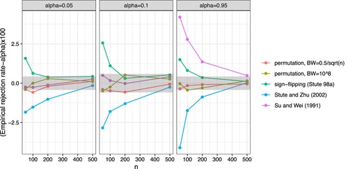
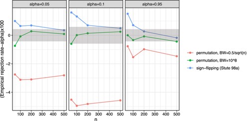
The results for different ${\theta }_1$ and ${\sigma }^2$ were very similar (data not shown), hence we show in Figure 1 the difference between the empirical rejection rate and the nominal level, α (choosing $\alpha =0.05$, 0.1 and 0.95 to give an overview over a wide range of αs) only for ${\theta }_1=1$ and ${\sigma }^2=1$. The performance of our proposed approach was good, regardless of the choice of the bandwidth, with the difference between the empirical rejection rate and the nominal level not exceeding the simulation margins of error regardless of the sample size, n. In contrast, the performance of the other approaches was not good with the difference between the empirical rejection rate and the nominal level exceeding the simulation margins of error unless when the sample size was large. Note that the results presented in Figure 1 imply that the distribution of the p-values when using the approaches proposed by Stute and Zhu [23], Lin et al. [3] and Stute et al. [24] are not uniform: the first approach is too conservative with the null hypothesis being rejected less often than the nominal level, the latter two approaches are too liberal rejecting the null hypothesis too often.

Figure 1. The difference between the empirical rejection rate and the nominal level, α, for some chosen values of $\alpha =0.05$, 0.1 and 0.95 (columns) for the example with normal homoscedastic random errors using ${\theta }_1=1$ and ${\sigma }^2=1$. Shaded areas are simulation margins of error. Different colours represent different approaches.

3.1.2. Normal heteroscedastic random errors.

Here we illustrate how the approaches perform in the presence of heteroscedasticity, with $e_i\sim N(0,{\sigma }_i^2)$, where ${\sigma }_i^2=(1+\psi x_{i1}{)}^2$. Different values of $\psi =-0.5$, $-0.25$, 0, 0.25, 0.5 were considered, using ${\theta }_1=1$.

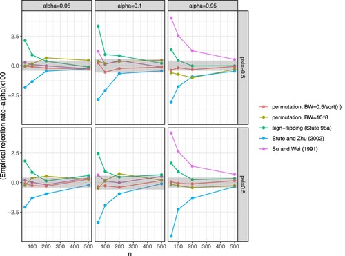
The results when using different values of ψ were similar (data not shown), hence we show in Figure 2 only the results for $\psi =-0.5$ and 0.5. The results were very similar to the example with normal homoscedastic random errors, with our proposed approach with bandwidth set to $0.5/\sqrt{n}$ attaining the nominal level and other approaches achieving this only when the sample size was large being too conservative (approach proposed by Stute and Zhu [23]) or too liberal (the approaches proposed by Lin et al. [3] and Stute et al. [24]) otherwise. As expected, setting the bandwidth to ${10}^8$ yielded slightly worse results than when using $0.5/\sqrt{n}$ with the former approach being slightly conservative for some values of ψ, however, the differences between the empirical rejection rate and the nominal level were not substantial.

Figure 2. The difference between the empirical rejection rate and the nominal level, α, for some chosen values of $\alpha =0.05$, 0.1 and 0.95 (columns) for the example with normal heteroscedastic random errors using different values of $\psi =-0.5$ and 0.5 (rows). Shaded areas are simulation margins of error. Different colours represent different approaches.

3.1.3. Non-normal homoscedastic random errors.

The size with non-normal random errors was checked with the example where $e_i={ϵ}_i-as$, ${ϵ}_i\sim \gamma (a,s)$ and a and s are the shape and the scale parameter of the gamma distribution ($\gamma (\cdot )$), respectively using ${\theta }_1=1$. The scale parameter was set to s = 1, while different values of the shape parameter were considered, a = 2, 4, 6, 8 and 10. Larger values of a mean that the distribution of the error term was more symmetric but also more variable.

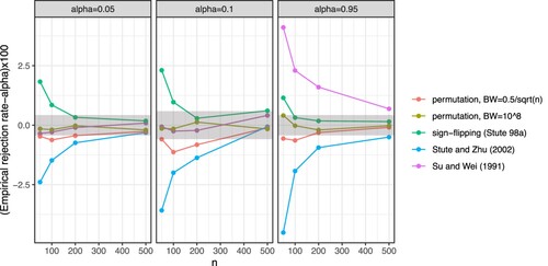
We show in Figure 3 only the results for a = 6 (the trends observed for other values of a were similar, data not shown). Our approach, setting the bandwidth to ${10}^8$, performed well attaining the nominal level; setting the bandwidth to $0.5/\sqrt{n}$ also performed well, but there were a few exceptions (the approach was slightly conservative with n<200). The performance of the other approaches was worse with the tests not attaining the nominal level for all values of α, especially with a smaller sample size (as in the previous examples the approach proposed by Stute and Zhu [23] was too conservative and the approaches proposed by Lin et al. [3] and Stute et al. [24] were too liberal).

Figure 3. The difference between the empirical rejection rate and the nominal level, α, for some chosen values of $\alpha =0.05$, 0.1 and 0.95 (columns) for the example with non-normal homoscedastic random errors using a = 6. Shaded areas are simulation margins of error. Different colours represent different approaches.

3.2. Omission of a quadratic effect or an interaction term

Here we illustrate the power to detect the lack-of-fit due to omitting the quadratic effect or the interaction term. The outcome variable was simulated from $y_i=1+x_{i1}+0.25x_{i2}+{\theta }_3{x}_{i3}+e_i,$ where $x_{i3}=x_{i1}^2$ or $x_{i3}=x_{i1}{x}_{i2}$, for the example where the quadratic and the interaction effects are omitted, respectively, and $e_i\sim N(0,0.1)$. Different values of ${\theta }_3=0$, 0.25, 0.50, 0.75, 1 were considered. 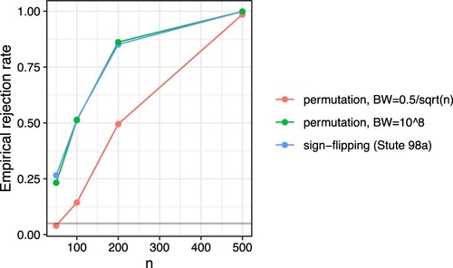Results for $\alpha =0.05$ and for different effect and sample sizes are reported in Figure 4 (power against the omission of the quadratic effect – lower panels, power against the omission of the interaction effect – upper panels; the results for n = 200 are omitted for brevity of the presentation).

Figure 4. Fraction rejected at $\alpha =0.05$ for different approaches under the null hypothesis (${\theta }_3=0$) and under different alternatives (omission of a quadratic term, omission of an interaction term; ${\theta }_3>0$) for various different sample sizes (n = 50, 100 and 500 columns). Shaded areas are simulation margins of error. Different colours represent different approaches.

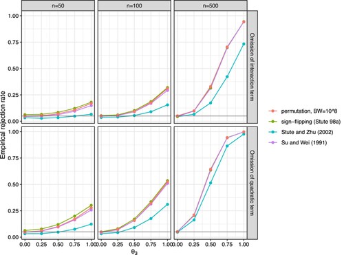
Judging from Figure 4 our approach performs well. As expected, the approach was more powerful when the effect size (${\theta }_3$) and sample size were larger. Setting the bandwidth to ${10}^8$ was slightly more powerful than using $0.5/\sqrt{n}$, but the differences were not substantial (results for $0.5/\sqrt{n}$ are not shown). The proposed approach was more powerful than the test proposed by Stute and Zhu [23], had similar power as the test proposed by Lin et al. [3] while the approach proposed by Stute et al. [24] was, with a smaller sample size, slightly more powerful, but the differences were not substantial. However, recall that the approaches proposed by Lin et al. [3] and Stute et al. [24] are too liberal rejecting the null hypothesis too often (see the results presented in the previous sections).

3.3. Nonlinear regression

Here we illustrate how our approach performs when applied to nonlinear regression. Here we only compare our approach with the approach proposed by Stute et al. [24], since it performed better than the other approaches in the previous examples. The outcome variable was simulated from the power model $y_i=2+15x_{i1}^{1/3}+e_i,$ where $e_i\sim N(0,1)$. The fitted model was the same as the simulated model. R function nls [37] was used to fit the model, using true values of the parameters as the starting values. The results are presented in Figure 5.

Figure 5. The difference between the empirical rejection rate and the nominal level, α, for some chosen values of $\alpha =0.05$, 0.1 and 0.95 (columns) for the nonlinear regression example where the fitted model was the same as the simulated model. Shaded areas are simulation margins of error. Different colours represent different approaches.

With a bandwidth set to $0.5/\sqrt{n}$ our approach was too conservative, however, when setting the bandwidth to ${10}^8$ the empirical rejection rates were within the simulation margins of error. The approach proposed by Stute et al. [24] was with a smaller sample size again too liberal.

To check the power of the proposed approach and compare it with the approach proposed by Stute et al. [24], the outcome variable was simulated from Michaelis–Menten model $y_i=2+15x_{i1}/(0.3+x_{i1})+e_i,$ where $e_i\sim N(0,1)$. The fitted model, however, assumed that the data were generated from the power model. Results are presented in Figure 6.

Figure 6. Fraction rejected at $\alpha =0.05$ for different approaches for the nonlinear regression example where the fitted and simulated models were different. Shaded areas are simulation margins of error. Different colours represent different approaches.

With bandwidth set to ${10}^8$ the power of our approach was larger than when using $0.5/\sqrt{n}$, and similar to the power obtained with the approach proposed by Stute et al. [24].

4. Application

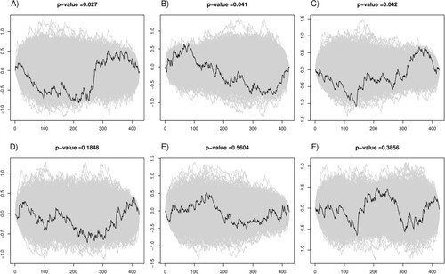
Our approach was applied to a dataset from a cross-sectional study of the dependence in daily activities among family practice non-attenders in Slovenia. We reanalysed a subset of data for 423 adult patients (aged 18 or over) requiring some level of assistance in their daily activities. We modelled the level of dependence in daily activities determined by a questionnaire through eight items, each on the 4-point Likert scale (dependence), exhibiting positively skewed distribution, and two covariates, patients age in years (age) and the assessment of pain intensity as determined by a questionnaire on a 10-point Likert scale (pain). First, we fitted a simple additive linear model using the OLS estimator and the results are shown in Figure 7, panels (A), (B) and (C). Our approach based on the CvM type test statistic, using Gaussian kernel with bandwidth set to $0.5/\sqrt{n}$, returned p-value of 0.027 and we can conclude that the fit of the model is poor (Figure 7, panel (A)). The tests using CvM type test statistic targeting at age and pain returned p-values equal to 0.041 and 0.042, respectively. From the plots of the constructed random process, we can conclude that the lack-of-fit due to covariate age is due to the omission of the quadratic term (Figure 7, panel (B), black curve). Based on Figure 7 panel (C), we then also modelled the covariate pain as a restricted cubic spline using the truncated power basis defining 3 knots. When modelling pain as a restricted cubic spline and age as a quadratic term, the p-value for the full model check was 0.185 and the null hypothesis was not rejected at $\alpha =0.05$ (Figure 7, panel D). The test using CvM type test statistic targeting at age and its square, returned a p-value of 0.560 and the test targeting at pain and its expanded term returned a p-value of 0.386 (Figure 7, panels (E) and (F), respectively) with the plots of the constructed process revealing an improved fit of the model.

Figure 7. The constructed random process (black curves) and 1000 randomly selected random processes which are obtained using the proposed permutation procedure (grey curves) for the dependence in daily activities dataset. The p-values are for the CvM type test statistic. Panel (A) refers to the model which includes only the main effects. Panels (B) and (C) are tests targeting at age and pain, respectively for the model which includes only the main effects. Panel (D) refers to the model which includes also the quadratic term of pain and models age as a restricted cubic spline with 3 knots. Panel (E) refers to the test targeting at age and its expanded term and panel (F) is for a test targeting at pain and its square.

5. Discussion

In practice, graphical procedures are mainly used to evaluate goodness-of-fit of the regression model. While these procedures are useful, they can be to a large extent subjective. They can be formalized by forming an empirical process based on residuals. Several goodness-of-fit tests based on such processes have been proposed. They are, however, very computationally expensive [24], target a certain fixed alternative [3,4], rely on the asymptotic independence of the residuals [22,27] or rely on some asymptotic properties of the constructed random process [3,23,26] and therefore can yield poor results with small sample size. We propose an approach that does not depend on the distribution of the errors and has the correct size also with a small sample size. This is achieved by using a novel permutation procedure to obtain the p-values. We prove that conditionally on the design matrix $\mathit{X}$, this approach is asymptotically consistent under the null and some alternative hypotheses.

In our approach, a consistent estimator of the function σ is required. In our simulation study, we used the standard Nadaraya–Watson estimator, where a kernel needs to be chosen and the bandwidth needs to be specified. It is well known that the choice of the kernel is not problematic [38]. We compared two options for setting the bandwidth, one used regularly in similar problems and one presenting the extreme case where σ is practically a constant. Both options gave a very similar result for the linear case (even with non-constant variance), showing some robustness of our approach against the choice of bandwidth. However, for the non-linear case using $0.5/\sqrt{n}$ did not yield good results, since our approach was too conservative having small power. In our particular example, this choice of bandwidth led to poor estimation of σ. With a larger bandwidth σ was estimated better and consequently, our approach performed well attaining the correct size while being as powerful as the approach proposed by Stute et al. [24] (which with a smaller sample size was too liberal in all our simulation examples). The question of how to consistently estimate the function σ in a general regression setting is, however, beyond the scope of this paper, see, e.g., Fan and Yao [39].

One potential disadvantage of using (any kind of) permutation (or bootstrap-based) testing could be a large computational burden. In the homoscedastic case, this was not an issue, as it is possible to implement the tests in a very efficient manner. For example, a typical simulated data example with two covariates, 1000 samples, and 10,000 permutations took 2.6 s using our R implementation. In comparison, the tests proposed by Lin et al. [3] using the gof package (no longer available on CRAN) with 10,000 simulations took 28.6 s for the same example. For the heteroscedastic case, the computational burden is increased by the calculation of $\hat{\sigma }$ and ${\hat{\sigma }}^{\ast }$, the latter of which must be performed many times. For example, when using 1000 permutations, the R implementation of the method takes about 10 s for data with n = 400 on a modern computer. In comparison, the implementation of our method written in Julia takes less than 40 ms on such data and the implementation in R for homoscedastic data takes around 130 milliseconds. With n = 1000 the R implementation for hetereoscedastic data takes about a minute, while the implementation in Julia takes less than 200 milliseconds. With n = 10, 000 the implementation in Julia is still manageable, taking about 20 s, while the R implementation is much slower, taking about 2.5 hours. Neither of these implementations is currently close to being optimal, but we do not expect this to be an important issue in practical research.

Acknowledgments

The dependence in daily activities data was provided by Zalika Klemenc Ketiš and Antonija Poplas Susič from the Health Centre Ljubljana. The dependence in daily activities data cannot be shared due to violating confidentiality. The constructive comments of two Reviewers are gratefully acknowledged.

Disclosure statement

No potential conflict of interest was reported by the author(s).

Additional information

Funding

Jakob Peterlin is a young researcher funded by the Slovene Research Agency (ARRS). The authors acknowledge the financial support by ARRS (Methodology for data analysis in medical sciences, P3-0154, and projects J3-1761 and N1-0035).

References

- González-Manteiga W, Crujeiras RM. An updated review of goodness-of-fit tests for regression models. TEST. 2013;22(3):361–411. doi:10.1007/s11749-013-0327-5.
- Stute W. Nonparametric model checks for regression. Ann Stat. 1997;25(2):613–641. doi:10.1214/aos/1031833666.
- Lin DY, Wei LJ, Ying Z. Model-checking techniques based on cumulative residuals. Biometrics. 2002;58(1):1–12. doi:10.1111/j.0006-341X.2002.00001.x.
- Solari A, Cessie S, Goeman JJ. Testing goodness of fit in regression: a general approach for specified alternatives. Stat Med. 2012;31(28):3656–3666. doi:10.1002/sim.5417.
- Khmaladze EV, Koul HL. Martingale transforms goodness-of-fit tests in regression models. Ann Stat. 2004;32(3):995–1034. doi:10.1214/009053604000000274.
- Khmaladze EV, Koul HL. Goodness-of-fit problem for errors in nonparametric regression: distribution free approach. Ann Stat. 2009;37(6A):3165–3185. doi:10.1214/08-AOS680.
- Beghin L, Orsingher E. On the maximum of the generalized Brownian bridge. Lith Math J. 1999;39(2):157–167. doi:10.1007/BF02469280.
- Kulperger R. On the distribution of the maximum of Brownian bridges with application to regression with correlated errors. J Stat Comput Simul. 1990;34(2-3):97–106. doi:10.1080/00949659008811209.
- Dwass M. Modified randomization tests for nonparametric hypotheses. Ann Math Stat. 1957;28(1):181–187. doi:10.1214/aoms/1177707045.
- Hemerik J, Goeman J. Exact testing with random permutations. TEST. 2018;27(4):811–825. doi:10.1007/s11749-017-0571-1.
- Phipson B, Smyth GK. Permutation P-values should never be zero: calculating exact P-values when permutations are randomly drawn. Stat Appl Genet Mol Biol. 2010;9(1):39.
- Ge Y, Dudoit S, Speed TP. Resampling-based multiple testing for microarray data analysis. Test. 2003;12(1):1–77.
- Lehmann EL, Romano JP. Testing statistical hypotheses. Vol. 3, New York, NY: Springer; 2005.
- DiCiccio CJ, Romano JP. Robust permutation tests for correlation and regression coefficients. J Am Stat Assoc. 2017;0:0–0. doi:10.1080/01621459.2016.1202117.
- Manly B. Randomization, bootstrap and Monte Carlo methods in biology. 3rd ed. New York, NY: Taylor & Francis; 2006.
- ter Braak CJF. Permutation versus bootstrap significance tests in multiple regression and Anova. Berlin, Heidelberg: Springer Berlin Heidelberg; 1992. doi:10.1007/978-3-642-48850-4_10. p. 79–85.
- Freedman D, Lane D. A nonstochastic interpretation of reported significance levels. J Bus Econ Stat. 1983;1(4):292–298. http://www.jstor.org/stable/1391660.
- Lepage R, Podgórski K. Resampling permutations in regression without second moments. J Multivar Anal. 1996;57(1):119–141. doi:10.1006/jmva.1996.0025. https://www.sciencedirect.com/science/article/pii/S0047259X96900251.
- Anderson MJ, Legendre P. An empirical comparison of permutation methods for tests of partial regression coefficients in a linear model. J Stat Comput Simul. 1999;62(3):271–303. doi:10.1080/00949659908811936.
- Anderson MJ, Robinson J. Permutation tests for linear models. Aust N Z J Stat. 2001;43(1):75–88. doi:10.1111/1467-842X.00156.
- Diebolt J, Zuber J. Goodness-of-fit tests for nonlinear heteroscedastic regression models. Stat Probab Lett. 1999;42(1):53–60. doi:10.1016/S0167-7152(98)00189-8. http://www.sciencedirect.com/science/article/pii/S0167715298001898.
- Fan J, Huang LS. Goodness-of-fit tests for parametric regression models. J Am Stat Assoc. 2001;96(454):640–652. doi:10.1198/016214501753168316.
- Stute W, Zhu LX. Model checks for generalized linear models. Scand J Stat. 2002;29(3):535–545. http://www.jstor.org/stable/4616730.
- Stute W, Gonzalez Manteiga W, Presedo Quindimil M. Bootstrap approximations in model checks for regression. J Am Stat Assoc. 1998;93(441):141–149. http://www.jstor.org/stable/2669611.
- Stute W, Thies S, Zhu LX. Model checks for regression: an innovation process approach. Ann Stat. 1998;26(5):1916–1934. doi:10.1214/aos/1024691363.
- Su JQ, Wei LJ. A lack-of-fit test for the mean function in a generalized linear model. J Am Stat Assoc. 1991;86(414):420–426. http://www.jstor.org/stable/2290587.
- Christensen R, Lin Y. Lack-of-fit tests based on partial sums of residuals. Commun Stat Theory Methods. 2015;44(13):2862–2880. doi:10.1080/03610926.2013.844256.
- Hardle W, Mammen E. Comparing nonparametric versus parametric regression fits. Ann Stat. 1993;21(4):1926–1947. doi:10.1214/aos/1176349403.
- Liu RY. Bootstrap procedures under some non-i.i.d. models. Ann Stat. 1988;16(4):1696–1708. doi:10.1214/aos/1176351062.
- Wu CFJ. Jackknife, bootstrap and other resampling methods in regression analysis. Ann Stat. 1986;14(4):1261–1295. doi:10.1214/aos/1176350142.
- Hattab MW, Christensen R. Lack of fit tests based on sums of ordered residuals for linear models. Aust N Z J Stat. 2018;60(2):230–257. doi:10.1111/anzs.12231.
- Christensen R, Sun SK. Alternative goodness-of-fit tests for linear models. J Am Stat Assoc. 2010;105(489):291–301. doi:10.1198/jasa.2009.tm08697.
- van der Vaart A, Wellner J. Weak convergence and empirical processes: with applications to statistics. New York, NY: Springer; 1996. (Springer Series in Statistics). https://books.google.si/books?id=OCenCW9qmp4C.
- Bishop Y, Light R, Mosteller F, et al. Discrete multivariate analysis: theory and practice. New York: Springer; 2007. https://books.google.si/books?id=IvzJz976rsUC.
- Vaart AW. Asymptotic statistics. New York, NY: Cambridge University Press; 2000. https://EconPapers.repec.org/RePEc:cup:cbooks:9780521784504.
- R Core Team. R: A Language and Environment for Statistical Computing. R Foundation for Statistical Computing, Vienna, Austria: 2014. http://www.R-project.org/.
- Bates D, Watts D. Nonlinear regression analysis, its applications. New York: Wiley; 1988. (Wiley series in probability and mathematical statistics). http://gso.gbv.de/DB=2.1/CMD?ACT=SRCHA&SRT=YOP&IKT=1016&TRM=ppn+025625357&sourceid=fbw_bibsonomy.
- Wand M, Jones M. Kernel smoothing. New York, NY: Taylor & Francis; 1994. (Chapman & Hall/CRC Monographs on Statistics & Applied Probability). https://books.google.si/books?id=GTOOi5yE008C.
- Fan J, Yao Q. Efficient estimation of conditional variance functions in stochastic regression. Biometrika. 1998;85(3):645–660. http://www.jstor.org/stable/2337393.