Predicting future failures in generalized order statistics and related models

Abstract

Quantile regression predictions are considered for generalized order statistics which extend results previously established for record values and order statistics. In order to derive the results, some (univariate and bivariate) distortion representations of generalized order statistics are established. In particular, prediction of the sth generalized order statistic $X_{(s)}^{\ast }$ based on F given a single (generalized) order statistic $X_{(r)}^{\ast }$ with r<s will be addressed. The presentation includes results for both known and unknown baseline distributions. In the latter case, we consider exponential distributions with unknown mean as well as the proportional hazards model. Using unimodality properties of the marginal density functions (pdf) of generalized order statistics, we find a simple representation of the maximum likelihood prediction of $X_{(s)}^{\ast }$ given $X_{(r)}^{\ast }$.

Keywords:

• Quantile regression prediction
• maximum likelihood prediction
• generalized order statistics
• record values
• exponential distribution

1. Introduction

The prediction of future failure times has been widely discussed in the literature assuming various scenarios for the data model. In particular, order statistics have been extensively used when the first r failure times $X_{(1)}^{\ast },\dots ,X_{(r)}^{\ast }$ are available in order to predict the value of a larger order statistic. Some basic ideas and concepts as well as references can be found in the monograph by David and Nagaraja [1, Section 8.7] (see also Arnold et al. [2, Section 7.6] and, for prediction intervals, Hahn et al. [3]). Various prediction concepts (like (best) linear prediction, (best) unbiased prediction, likelihood prediction and Bayesian prediction) have been used in this area. A brief review on point prediction methods applied under progressive censoring can be found in Balakrishnan and Cramer [4, Chapter 16] which also includes references to related results in terms of generalized order statistics. Further references dealing with this problem can be found in, e.g. Navarro [5], Navarro and Buono [6], Volovskiy [7], and Volovskiy and Kamps [8].

In this paper, we consider quantile regression predictions which have been discussed in Navarro [5] for record values and in Navarro and Buono [6] for order statistics, respectively. We extend this approach to generalized order statistics which covers progressive censoring as a particular case. In order to establish the corresponding representations, we provide the necessary extensions to generalized order statistics in Section 2 (for details on generalized order statistics and related results, see Kamps [9], Cramer and Kamps [10]). In Section 3, we establish some (bivariate) distortion representation of generalized order statistics which will be utilized in Section 4 to obtain quantile regression predictions. We consider prediction of the sth (generalized) order statistic $X_{(s)}^{\ast }$ based on F and some parameters ${\gamma }_1,{\gamma }_2,\dots$ given a single (generalized) order statistic $X_{(r)}^{\ast }$ (r<s). First, we study the case of a known baseline distribution. Then, we consider the case of exponential distributions with unknown mean. Using unimodality properties of the density functions (pdf) of generalized order statistics, we find a simple representation of the maximum likelihood prediction (according to Kaminsky and Rhodin [11]) of $X_{(s)}^{\ast }$ given $X_{(r)}^{\ast }$. In particular, we show that the point predictor can be written as ${\hat{X}}_{(s)}^{\ast }=X_{(r)}^{\ast }+m_{{\gamma }_{r+1},\dots ,{\gamma }_s}/{\hat{\vartheta }}_{\mathrm{MLE}}$where $m_{{\gamma }_{r+1},\dots ,{\gamma }_s}$ is the mode of a function related to the density function of the $(s-r)$th generalized order statistic based on a uniform distribution and parameters ${\gamma }_{r+1}+1,\dots ,{\gamma }_s+1$ (see Equation (7(7) ${\kappa }_{{\gamma }_{r+1},\dots ,{\gamma }_s}(z)={\mathrm{e}}^{-z}{g}_{s-r}({\mathrm{e}}^{-z};{\gamma }_{r+1},\dots ,{\gamma }_s)=g_{s-r}({\mathrm{e}}^{-z};{\gamma }_{r+1}+1,\dots ,{\gamma }_s+1),$(7) )) and ${\hat{\vartheta }}_{\mathrm{MLE}}$ denotes the MLE based on the single observation $X_{(r)}^{\ast }$. Furthermore, we consider the particular cases of order statistics, ℓ-generalized order statistics, and record values and discuss the value of $m_{{\gamma }_{r+1},\dots ,{\gamma }_s}$ in these models. Using the representation of the MLE based on a single generalized order statistic, we conclude from the above representation that the maximum likelihood predictor can be written in the form ${\hat{X}}_{(s)}^{\ast }=c_{(r,s)}{X}_{(r)}^{\ast },$where $c_{(r,s)}$ depends only on the model parameters of the generalized order statistics (see Sections 4.2.1 and 4.2.2).

An extension to proportional hazard rate models is also presented. Finally, the results are illustrated by a couple of examples and simulations in Section 5.

Throughout, we use the following parametric representations for the pdf of

1. an exponential distribution with parameter $\vartheta >0$ (for short $\mathrm{Exp}(\vartheta )$-distribution): $f(t)={\mathrm{e}}^{-t/\vartheta }/\vartheta$, $t\ge 0$,

2. a gamma distribution with parameters $\beta >0,\vartheta >0$ (for short $\mathsf{\text{Gamma}}(\beta ,\vartheta )$-distribution): $f(t)=\frac{1}{\mathrm{\Gamma }(\beta ){\vartheta }^{\beta }}{t}^{\beta -1}{\mathrm{e}}^{-t/\vartheta }$, $t\ge 0$,

3. a beta distribution with parameters $\alpha ,\beta >0$ (for short $\mathsf{\text{beta}}(\alpha ,\beta )$-distribution): $f(t)=\frac{\mathrm{\Gamma }(\alpha )\mathrm{\Gamma }(\beta )}{\mathrm{\Gamma }(\alpha +\beta )}{t}^{\alpha -1}(1-t{)}^{\beta -1}$, $t\in (0,1)$,

where $\mathrm{\Gamma }(\cdot )$ denotes the gamma function.

2. Preliminaries

For $U_1,\dots ,U_m\stackrel{\mathrm{iid}}{\sim }U(0,1)$, let $U_{(k)}^{\ast }=1-\prod _{j=1}^k{U}_j^{1/{\gamma }_j}$, $1\le k\le m$. According to Cramer and Kamps [10] generalized order statistics $X_{(1)}^{\ast },\dots ,X_{(m)}^{\ast }$ based on a cdf F and parameters ${\gamma }_1,\dots ,{\gamma }_m>0$, can be defined by the stochastic representation (1) $X_{(k)}^{\ast }=F^{\leftarrow }(U_{(k)}^{\ast })=F^{\leftarrow }(1-\prod _{j=1}^k{U}_j^{1/{\gamma }_j})={\overline{F}}^{\leftarrow }\left(\prod _{j=1}^k{U}_j^{1/{\gamma }_j}\right),k=1,\dots ,m,$(1) where $F^{\leftarrow }$ defines the quantile function of F, that is, $F^{\leftarrow }(y)=inf\{x:F(x)\ge y\},y\in (0,1),$and ${\overline{F}}^{\leftarrow }(\cdot )=F^{\leftarrow }(1-\cdot )$ denotes the (pseudo) inverse function of the reliability function $\overline{F}=1-F$. On the other hand, such representations like (1(1) $X_{(k)}^{\ast }=F^{\leftarrow }(U_{(k)}^{\ast })=F^{\leftarrow }(1-\prod _{j=1}^k{U}_j^{1/{\gamma }_j})={\overline{F}}^{\leftarrow }\left(\prod _{j=1}^k{U}_j^{1/{\gamma }_j}\right),k=1,\dots ,m,$(1) ) hold for order statistics, record values, and progressively Type-II censored order statistics as well as sequential order statistics by choosing appropriate values for the parameters ${\gamma }_j$ (see Cramer and Kamps [12], Balakrishnan and Cramer [4]). For order statistics, this result has also been derived by Malmquist [13]. Clearly, simulation of $U_{(k)}^{\ast }$ (and $X_{(k)}^{\ast }$) is easily possible using the product representation in (1(1) $X_{(k)}^{\ast }=F^{\leftarrow }(U_{(k)}^{\ast })=F^{\leftarrow }(1-\prod _{j=1}^k{U}_j^{1/{\gamma }_j})={\overline{F}}^{\leftarrow }\left(\prod _{j=1}^k{U}_j^{1/{\gamma }_j}\right),k=1,\dots ,m,$(1) ).

In the following, we denote by $G_d(\cdot ;{\eta }_1,\dots ,{\eta }_d)$ the cdf of a product $\prod _{j=1}^d{U}_j^{1/{\eta }_j}$ as in (1(1) $X_{(k)}^{\ast }=F^{\leftarrow }(U_{(k)}^{\ast })=F^{\leftarrow }(1-\prod _{j=1}^k{U}_j^{1/{\gamma }_j})={\overline{F}}^{\leftarrow }\left(\prod _{j=1}^k{U}_j^{1/{\gamma }_j}\right),k=1,\dots ,m,$(1) ) with parameters ${\eta }_1,\dots ,{\eta }_d>0$. Notice that $G_d(\cdot ;{\eta }_1,\dots ,{\eta }_d)$ is continuous and strictly increasing on $(0,1)$. Then, for $1\le r<s\le m$, we get (2) $W_{(r,s:m)}=\frac{\overline{F}(X_{(s)}^{\ast })}{\overline{F}(X_{(r)}^{\ast })}=\frac{\prod _{j=1}^s{U}_j^{1/{\gamma }_j}}{\prod _{j=1}^r{U}_j^{1/{\gamma }_j}}=\prod _{j=r+1}^s{U}_j^{1/{\gamma }_j},$(2) so that we have $Pr(W_{(r,s:m)}\le t)=G_{s-r}(t;{\gamma }_{r+1},\dots ,{\gamma }_s),t\in \mathbb{R}.$It should be noted that the above considerations show that the identity (3) $X_{(s)}^{\ast }={\overline{F}}^{\leftarrow }(W_{(r,s:m)}\overline{F}(X_{(r)}^{\ast }))$(3) holds where $W_{(r,s:m)}$ and $X_{(r)}^{\ast }$ are independent random variables. This illustrates the Markovian property and shows that $X_{(s)}^{\ast }$ can be seen as a somewhat (randomly) scaled version of $X_{(r)}^{\ast }$. The connection given in (3(3) $X_{(s)}^{\ast }={\overline{F}}^{\leftarrow }(W_{(r,s:m)}\overline{F}(X_{(r)}^{\ast }))$(3) ) is a key point for the results obtained in the present paper. A graphical illustration of the iterative construction can be found in Cramer [14].

Remark 2.1

In case of order statistics, the gammas are given by ${\gamma }_j=n-j+1$, $1\le j\le n$. Then, $W_{(r,s:m)}$ has a $\mathsf{\text{beta}}(n-s+1,s-r)$-distribution which can be seen from a result of Rao [15] since $U_j^{1/{\gamma }_j}\sim \mathsf{\text{beta}}(n-j+1,1)$ (see also Cramer [16], Bdair and Raqab [17]). For record values, that is, ${\gamma }_j=1$ for all j, one has that $W_{(r,s:m)}=\prod _{j=r+1}^s{U}_j$. Hence, the distribution of $W_{(r,s:m)}$ equals that of a product of s−r independent standard uniform random variables. In particular, $-\ln W_{(r,s:m)}\sim \mathsf{\text{Gamma}}(s-r,1)$ has a gamma distribution (see Navarro [5]).

Remark 2.2

For illustration, we provide an expression for $G_{s-r}$ when $s-r\in \{1,2\}$.

1. The case s = r + 1 is trivial and we have $G_1(u;{\gamma }_1)=Pr(U_1^{1/{\gamma }_1}\le u)=u^{{\gamma }_1}$for $u\in [0,1]$ (i.e., it is a power (or beta) distribution).

2. In the case s = r + 2, we can also get explicit expressions. If ${\gamma }_1\ne {\gamma }_2$, then a straightforward calculation leads to $G_2(u;{\gamma }_1,{\gamma }_2)=\frac{{\gamma }_1}{{\gamma }_1-{\gamma }_2}{u}^{{\gamma }_2}-\frac{{\gamma }_2}{{\gamma }_1-{\gamma }_2}{u}^{{\gamma }_1}$for $u\in [0,1]$ (i.e., it is a negative mixture of two power distributions). If ${\gamma }_1={\gamma }_2$, then $G_2(u;{\gamma }_1,{\gamma }_2)=u^{{\gamma }_1}-u^{{\gamma }_1}\ln \left(u^{{\gamma }_1}\right)$for $u\in [0,1]$ (i.e., it is a distorted distribution of a power distribution with the dual distortion function of a minimal repair process or an upper record).

Generally, the distribution of $W_{(r,s:m)}=\prod _{j=r+1}^s{U}_j^{1/{\gamma }_j}$ can be obtained easily from a log-transformation, that is, $-\ln W_{(r,s:m)}=\sum _{j=r+1}^s\frac{1}{{\gamma }_j}(-\ln U_j)=\sum _{j=r+1}^s\frac{Z_j}{{\gamma }_j},$where $Z_1,\dots ,Z_m\stackrel{\mathrm{iid}}{\sim }\mathrm{Exp}(1)$. Hence, the distribution of $-\ln W_{(r,s:m)}$ equals the distribution of a generalized order statistic based on parameters ${\gamma }_{r+1},\dots ,{\gamma }_s$ and a standard exponential distribution (or the sum of independent but possibly not identically exponentially distributed random variables). Explicit representations for the pdf and cdf can be found in Kamps and Cramer [18] and Cramer and Kamps [10] (see also Springer and Thompson [19], Springer [20], Botta et al. [21], Mathai [22], Akkouchi [23], and Levy [24]). They are particularly simple in case that

1. γ's are all equal to γ which means that $-\ln W_{(r,s:m)}\sim \mathsf{\text{Gamma}}(s-r,1/\gamma )$;

2. γ's are all different. In this case, the cdf of $-\ln W_{(r,s:m)}$ is given by (4) $\begin{array}{rl}{F}_{\ast ,r,s}^{({\gamma }_{r+1},\dots ,{\gamma }_s)}(t)& =1-(-1{)}^{s-r-1}\left(\prod _{j=r+1}^s{\gamma }_j\right)\sum _{j=r+1}^s{\gamma }_j^{-1}(\prod _{\begin{array}{c}k=r+1\\ v\ne j\end{array}}^s({\gamma }_j-{\gamma }_k{)}^{-1}){\mathrm{e}}^{-{\gamma }_{j}t},\\ & t\ge 0.\end{array}$(4)

In general, the cdf can also be presented in terms of divided differences as has been pointed out in Cramer [25] and Levy [24].

Remark 2.3

Notice that, for parameters ${\gamma }_{r+1},\dots ,{\gamma }_s$, the pdf of the log-transformed random variable $-\ln W_{(r,s:m)}\stackrel{d}{=}\sum _{i=1}^{s-r}{Z}_i/{\gamma }_{r+i}$ is given by (5) ${\kappa }_{{\gamma }_{r+1},\dots ,{\gamma }_s}(z)={\mathrm{e}}^{-z}{g}_{s-r}(e^{-z};{\gamma }_{r+1},\dots ,{\gamma }_s),z\ge 0,$(5) and is log-concave and, thus, unimodal (see Cramer [26] as well as Cramer et al. [27]). Moreover, as pointed out in Cramer [26], $W_{(r,s:m)}$ is multiplicative strongly unimodal (see Cuculescu and Theodorescu [28]) which also implies unimodality.

From Cramer et al. [27], the limits (6) $\underset{z\to \mathrm{\infty }}{lim}{\kappa }_{{\gamma }_{r+1},\dots ,{\gamma }_s}(z)=0,\underset{z\to 0}{lim}{\kappa }_{{\gamma }_{r+1},\dots ,{\gamma }_s}(z)={\kappa }_{{\gamma }_{r+1},\dots ,{\gamma }_s}(0)=\{\begin{array}{ll}{\gamma }_{r+1},& r+1=s\\ 0,& r+1<s\end{array}$(6) can be obtained which show that, for s>r + 1, the maximum of ${\kappa }_{{\gamma }_{r+1},\dots ,{\gamma }_s}$ is attained at an inner point of the interval $[0,\mathrm{\infty })$. For r + 1 = s, the maximum is attained at zero. The latter identity in (6(6) $\underset{z\to \mathrm{\infty }}{lim}{\kappa }_{{\gamma }_{r+1},\dots ,{\gamma }_s}(z)=0,\underset{z\to 0}{lim}{\kappa }_{{\gamma }_{r+1},\dots ,{\gamma }_s}(z)={\kappa }_{{\gamma }_{r+1},\dots ,{\gamma }_s}(0)=\{\begin{array}{ll}{\gamma }_{r+1},& r+1=s\\ 0,& r+1<s\end{array}$(6) ) can be obtained using expressions for pdfs of uniform generalized order statistics in terms of Meijer's G-functions (see Cramer et al. [27], Lemma 2.1 (iv)), that is, (7) ${\kappa }_{{\gamma }_{r+1},\dots ,{\gamma }_s}(z)={\mathrm{e}}^{-z}{g}_{s-r}({\mathrm{e}}^{-z};{\gamma }_{r+1},\dots ,{\gamma }_s)=g_{s-r}({\mathrm{e}}^{-z};{\gamma }_{r+1}+1,\dots ,{\gamma }_s+1),$(7) as well as the limits for $g_{s-r}$ in Lemma 2.2 (v) of Cramer et al. [27]. This property will be used when considering predictions with unknown baseline distribution.

Log-concavity of the pdf of $W_{(r,s:m)}$ holds when, e.g., the ordered parameters ${\gamma }_{(r+1)}\le \cdots \le {\gamma }_{(s)}$ satisfy $1\le {\gamma }_{(r+1)}$ and the difference of successive ${\gamma }_{(i)}$'s is at least 1. The latter one is true, for instance, for order statistics and progressively Type-II censored order statistics but not for record values. Furthermore, the moments of $W_{(r,s:m)}$ can be easily obtained from (2(2) $W_{(r,s:m)}=\frac{\overline{F}(X_{(s)}^{\ast })}{\overline{F}(X_{(r)}^{\ast })}=\frac{\prod _{j=1}^s{U}_j^{1/{\gamma }_j}}{\prod _{j=1}^r{U}_j^{1/{\gamma }_j}}=\prod _{j=r+1}^s{U}_j^{1/{\gamma }_j},$(2) ). In particular, for $\ell >0$, (8) $E(W_{(r,s:m)}^{\ell })=\prod _{j=r+1}^{s}E(U_j^{\ell /{\gamma }_j})=\prod _{j=r+1}^s\frac{{\gamma }_j}{\ell +{\gamma }_j},$(8) which yields directly $E(W_{(r,s:m)})=\prod _{j=r+1}^s\frac{{\gamma }_j}{1+{\gamma }_j}$.

3. Distortion representations

The key result for the predictions could be presented as follows. It will be used to establish the conditional predictive likelihood function ($\mathsf{PLF}$) of $X_{(s)}^{\ast }$ given $X_{(r)}^{\ast }$. An expression of the respective pdf can be found in, e.g., Cramer [16, Theorem 3.3.2] (see also (10(10) $f_{r,s:m}(y\mid x)=\frac{f(y)}{\overline{F}(x)}{g}_{s-r}(\frac{\overline{F}(y)}{\overline{F}(x)};{\gamma }_{r+1},\dots ,{\gamma }_s),y\ge x,$(10) )).

Theorem 3.1

Let F be a continuous cdf. With the notation introduced above, the conditional reliability function of $(X_{(s)}^{\ast }\mid X_{(r)}^{\ast }=x)$ is (9) ${\overline{F}}_{s|r:m}(y\mid x)=G_{s-r}(\frac{\overline{F}(y)}{\overline{F}(x)};{\gamma }_{r+1},\dots ,{\gamma }_s)$(9) for $1\le r<s\le m$ and x and y such that $\overline{F}(x)>0$ and $y\ge x$.

Proof.

The result follows directly from the structure of generalized order statistics (see Cramer [29]). First we note that, from (2(2) $W_{(r,s:m)}=\frac{\overline{F}(X_{(s)}^{\ast })}{\overline{F}(X_{(r)}^{\ast })}=\frac{\prod _{j=1}^s{U}_j^{1/{\gamma }_j}}{\prod _{j=1}^r{U}_j^{1/{\gamma }_j}}=\prod _{j=r+1}^s{U}_j^{1/{\gamma }_j},$(2) ) and (3(3) $X_{(s)}^{\ast }={\overline{F}}^{\leftarrow }(W_{(r,s:m)}\overline{F}(X_{(r)}^{\ast }))$(3) ), we get $\overline{F}(X_{(s)}^{\ast })=\prod _{j=1}^s{U}_j^{1/{\gamma }_j}=W_{(r,s:m)}\overline{F}(X_{(r)}^{\ast }),$where $W_{(r,s:m)}=\prod _{j=r+1}^s{U}_j^{1/{\gamma }_j}$ and $\overline{F}(X_{(r)}^{\ast })=\prod _{j=1}^r{U}_j^{1/{\gamma }_j}$ are independent. Therefore, for $\overline{F}(x)>0$ and $y\ge x$, $\begin{array}{rl}{\overline{F}}_{s|r:m}(y\mid x)& =Pr(X_{(s)}^{\ast }>y\mid X_{(r)}^{\ast }=x)\\ & =Pr(\overline{F}(X_{(s)}^{\ast })\le \overline{F}(y)\mid X_{(r)}^{\ast }=x)\\ & =Pr(\frac{\overline{F}(X_{(s)}^{\ast })}{\overline{F}(X_{(r)}^{\ast })}\le \frac{\overline{F}(y)}{\overline{F}(x)}\mid X_{(r)}^{\ast }=x)\\ & =Pr(W_{(r,s:m)}\le \frac{\overline{F}(y)}{\overline{F}(x)}\mid X_{(r)}^{\ast }=x)\\ & =Pr(W_{(r,s:m)}\le \frac{\overline{F}(y)}{\overline{F}(x)})\\ & =G_{s-r}(\frac{\overline{F}(y)}{\overline{F}(x)};{\gamma }_{r+1},\dots ,{\gamma }_s).\end{array}$This proves the representation in (9(9) ${\overline{F}}_{s|r:m}(y\mid x)=G_{s-r}(\frac{\overline{F}(y)}{\overline{F}(x)};{\gamma }_{r+1},\dots ,{\gamma }_s)$(9) ).

The representation in (9(9) ${\overline{F}}_{s|r:m}(y\mid x)=G_{s-r}(\frac{\overline{F}(y)}{\overline{F}(x)};{\gamma }_{r+1},\dots ,{\gamma }_s)$(9) ) can be written as a distortion representation for the spacing $(X_{(s)}^{\ast }-x\mid X_{(r)}^{\ast }=x)$ whose reliability function can be written as $Pr(X_{(s)}^{\ast }-x>t\mid X_{(r)}^{\ast }=x)=G_{s-r}(\frac{\overline{F}(x+t)}{\overline{F}(x)};{\gamma }_{r+1},\dots ,{\gamma }_s)=q({\overline{F}}_x(t))$for $t\ge 0$, where $q(\cdot )=G_{s-r}(\cdot ;{\gamma }_{r+1},\dots ,{\gamma }_s)$ is a distortion function (i.e., a continuous distribution function with support included in $(0,1)$) and ${\overline{F}}_x(t)=\frac{\overline{F}(t+x)}{\overline{F}(x)}$, $x,t\ge 0$, is the reliability function of the residual lifetime at age x. So all the results for distortions can be directly applied to it (see, e.g., Navarro [30]).

We can also obtain a bivariate distortion representation for the distribution of the bivariate random vector $(X_{(r)}^{\ast },X_{(s)}^{\ast })$, $1\le r<s\le m$. For the definition and properties of bivariate distortions see [31].

Theorem 3.2

Let F be continuous. With the notation introduced above, the joint reliability function of $(X_{(r)}^{\ast },X_{(s)}^{\ast })$ is given by ${\overline{F}}_{r,s:m}(x,y)=D(\overline{F}(x),\overline{F}(y))$for $1\le r<s\le m$, where D is a bivariate distortion function which depends on $r,s,{\gamma }_1,\dots ,{\gamma }_s$. Moreover, $\begin{array}{rl}D(u,v)& =\{\begin{array}{ll}{G}_r(v;{\gamma }_1,\dots ,{\gamma }_r)& \\ +{\displaystyle {\int }_v^u{G}_{s-r}(\frac{v}{w};{\gamma }_{r+1},\dots ,{\gamma }_s)g_r(w;{\gamma }_1,\dots ,{\gamma }_r)\mathrm{d}w}& \\ & \mathrm{for}0\le v\le u\le 1\\ G_r(u;{\gamma }_1,\dots ,{\gamma }_r)& \mathrm{for}0\le u<v\le 1\end{array}\\ & =G_r(u\wedge v;{\gamma }_1,\dots ,{\gamma }_r)\\ & +{\mathbb{1}}_{(0,u)}(v){\int }_v^u{G}_{s-r}(\frac{v}{w};{\gamma }_{r+1},\dots ,{\gamma }_s)g_r(w;{\gamma }_1,\dots ,{\gamma }_r)\mathrm{d}w,\end{array}$where $u\wedge v=min(u,v)$ and $g_r$ is the pdf of $G_r$. In particular, we get the corresponding pdf $d(u,v)=\frac{1}{u}{g}_{s-r}(\frac{v}{u};{\gamma }_{r+1},\dots ,{\gamma }_s)g_r(u;{\gamma }_1,\dots ,{\gamma }_r),0\le v\le u\le 1,$and zero elsewhere.

Proof.

Let D be the joint distribution function of $U=\overline{F}(X_{(r)}^{\ast })$ and $V=\overline{F}(X_{(s)}^{\ast })$. As its support is $(0,1{)}^2$ it is a bivariate distortion function (see Navarro et al. [31]). Therefore, $\begin{array}{rl}{\overline{F}}_{r,s:m}(x,y)& =Pr(X_{(r)}^{\ast }>x,X_{(s)}^{\ast }>y)\\ & =Pr(\overline{F}(X_{(r)}^{\ast })\le \overline{F}(x),\overline{F}(X_{(s)}^{\ast })\le \overline{F}(y))\\ & =D(\overline{F}(x),\overline{F}(y)).\end{array}$Moreover, for $0\le v\le u\le 1$, we have for $U=\prod _{j=1}^r{U}_j^{1/{\gamma }_j}$ and $V=\prod _{j=1}^s{U}_j^{1/{\gamma }_j}=U\cdot \prod _{j=r+1}^s{U}_j^{1/{\gamma }_j}$ $\begin{array}{rl}D(u,v)& =Pr(U\le u,V\le v)\\ & ={\int }_0^{u}Pr(V\le v\mid U=w)g_r(w;{\gamma }_1,\dots ,{\gamma }_r)\mathrm{d}w\\ & ={\int }_0^{u}Pr(\prod _{r+1}^s{U}_j^{1/{\gamma }_j}\le \frac{v}{w}\mid U=w)g_r(w;{\gamma }_1,\dots ,{\gamma }_r)\mathrm{d}w\\ & ={\int }_0^{u}Pr(\prod _{r+1}^s{U}_j^{1/{\gamma }_j}\le \frac{v}{w})g_r(w;{\gamma }_1,\dots ,{\gamma }_r)\mathrm{d}w\\ & ={\int }_0^v{g}_r(w;{\gamma }_1,\dots ,{\gamma }_r)\mathrm{dw}+{\int }_v^u{G}_{s-r}(\frac{v}{w};{\gamma }_{r+1},\dots ,{\gamma }_s)g_r(w;{\gamma }_1,\dots ,{\gamma }_r)\mathrm{d}w\\ & =G_r(v;{\gamma }_1,\dots ,{\gamma }_r)+{\int }_v^u{G}_{s-r}(\frac{v}{w};{\gamma }_{r+1},\dots ,{\gamma }_s)g_r(w;{\gamma }_1,\dots ,{\gamma }_r)\mathrm{d}w.\end{array}$For $0\le u<v\le 1$, we get $D(u,v)=Pr(U\le u,V\le v)=Pr(U\le u)=G_r(u;{\gamma }_1,\dots ,{\gamma }_r)$since V<U. The expression for the pdf d is directly obtained from the presented representation of the cdf D by, e.g., differentiating D with respect to u and v.

Remark 3.3

If we are able to get an explicit expression for D (which is not easy in general), then we can apply all the results included in Navarro et al. [31]. In particular, we could predict $X_{(r)}^{\ast }$ from $X_{(s)}^{\ast }=x$ for $1\le r<s\le m$. This kind of predictions is not as common as that considered in Theorem 3.1 since, if we work with lifetimes, we usually have information about early failures $X_{(r)}^{\ast }$ and we want to predict future failures $X_{(s)}^{\ast }$ for s>r. In this case, we have information about a current failure $X_{(s)}^{\ast }$ at time x and we want to predict a past failure $X_{(r)}^{\ast }$.

4. Quantile regression predictions

4.1. Predictions when F is supposed known

Theorem 3.1 allows us to predict $X_{(s)}^{\ast }$ from $X_{(r)}^{\ast }=x$ by using the median regression curve m which is obtained by solving the equation (in y) $G_{s-r}(\frac{\overline{F}(y)}{\overline{F}(x)};{\gamma }_{r+1},\dots ,{\gamma }_s)=\mathrm{0.5.}$Denoting by $q_{0.5}$ the unique median of this cdf, the median regression curve is given by $m(x)={\overline{F}}^{\leftarrow }(q_{0.5}\overline{F}(x)).$which for order statistics leads to the result given in Navarro and Buono [6].

This prediction can be reinforced with the following prediction bands. If we want to get $Pr(X_{(s)}^{\ast }\in I_{\alpha ,\beta }(x)\mid X_{(r)}^{\ast }=x)=\beta -\alpha$for some $0\le \alpha <\beta \le 1$, then $I_{\alpha ,\beta }(x)=[{\overline{F}}^{\leftarrow }(q_{\beta }\overline{F}(x)),{\overline{F}}^{\leftarrow }(q_{\alpha }\overline{F}(x))],$where $q_{\alpha }$ and $q_{\beta }$ are the unique α and β quantiles of $G_{s-r}(\cdot ;{\gamma }_{r+1},\dots ,{\gamma }_s)$. For example, the $90\mathrm{\%}$ centred prediction band is obtained as $I_{0.05,0.95}(x)=[{\overline{F}}^{\leftarrow }(q_{0.95}\overline{F}(x)),{\overline{F}}^{\leftarrow }(q_{0.05}\overline{F}(x))].$In other cases, we could prefer bottom prediction bands obtained as $I_{0.1,1}(x)=[x,{\overline{F}}^{\leftarrow }(q_{0.1}\overline{F}(x))].$Numerical methods can be used to determine these quantiles. Here we could also plot the level curves $G_{s-r}(\frac{\overline{F}(y)}{\overline{F}(x)};{\gamma }_{r+1},\dots ,{\gamma }_s)=p$for, e.g., p = 0.05, 0.25, 0.5, 0.75, 0.95.

Another option is to consider the mode, that is, the maximum likelihood predictor (MLP). The conditional pdf can be obtained from Theorem 3.1 as (10) $f_{r,s:m}(y\mid x)=\frac{f(y)}{\overline{F}(x)}{g}_{s-r}(\frac{\overline{F}(y)}{\overline{F}(x)};{\gamma }_{r+1},\dots ,{\gamma }_s),y\ge x,$(10) where f and $g_{s-r}$ are the pdf of F and $G_{s-r}$. To get the MLP we must look for the maximum of this function for fixed values of x and the gamma parameters.

Another reasonable option could be to consider the unique mode $m_o$ of $G_{s-r}$ which leads to the predictor $m_{\mathrm{mode}}(x)={\overline{F}}^{\leftarrow }(m_o\overline{F}(x)).$In this regard, knowledge about the shapes of the density functions could be helpful. These shapes have been completely characterized by Bieniek [32] for uniform generalized order statistics, that is, for arbitrary (positive) γ's. For progressively Type-II censored order statistics, the possible shapes reduce significantly (see Balakrishnan and Cramer [4, Theorem 2.7.5]). These results are helpful in finding the mode. However, the maximum of the density function has to be computed numerically by standard methods like Newton–Raphson, Nelder–Mead procedures etc.

The third option is to consider the mean of $W_{(r,s:m)}$ (see (8(8) $E(W_{(r,s:m)}^{\ell })=\prod _{j=r+1}^{s}E(U_j^{\ell /{\gamma }_j})=\prod _{j=r+1}^s\frac{{\gamma }_j}{\ell +{\gamma }_j},$(8) )) so that the corresponding predictor is given by (11) $m_{\mathrm{mean}}(x)={\overline{F}}^{\leftarrow }(\overline{F}(x)\prod _{j=r+1}^s\frac{{\gamma }_j}{1+{\gamma }_j}).$(11) This method is equivalent to consider the regression curve of $\overline{F}(X_{(s)})$ given by $\begin{array}{rl}E(\overline{F}(X_{(s)})\mid X_{(r)}=x)& =E(W_{(r,s:m)}\overline{F}(X_{(r)})\mid X_{(r)}=x)\\ & =\overline{F}(x)E(W_{(r,s:m)}\mid X_{(r)}=x)\\ & =\overline{F}(x)\prod _{j=r+1}^s\frac{{\gamma }_j}{1+{\gamma }_j}.\end{array}$Of course, in general, $m_{\mathrm{mean}}$ is different from the real regression curve $E(X_{(s)}\mid X_{(r)}=x)$.

4.2. Inferential approaches when F contains unknown parameters

If $(F_{\theta }{)}_{\theta \in \mathrm{\Theta }}$ forms a parametric family of absolutely continuous distributions with unknown parameters $\theta \in \mathrm{\Theta }\subseteq {\mathbb{R}}^p$, the likelihood function of the first r generalized order statistics $X_{(1)}^{\ast },\dots ,X_{(r)}^{\ast }$ and data $x_1,\dots ,x_r$ is given by $L(\theta )=\left(\prod _{j=1}^r{\gamma }_j\right)f_{\theta }(x_r){\overline{F}}_{\theta }^{{\gamma }_r-1}(x_r)\prod _{j=1}^{r-1}{f}_{\theta }(x_j){\overline{F}}_{\theta }^{{\gamma }_j-{\gamma }_{j+1}-1}(x_j).$Assuming a proportional hazard rate (PHR) model with known baseline cdf $F_0$ and parameter $\vartheta >0$, that is, ${\overline{F}}_{\vartheta }={\overline{F}}_0^{\vartheta }$, $L(\vartheta )=\left(\prod _{j=1}^r{\gamma }_j\right){\vartheta }^r{f}_0(x_r){\overline{F}}_0^{{\gamma }_r\vartheta -1}(x_r)\prod _{j=1}^{r-1}{f}_0(x_j){\overline{F}}_0^{({\gamma }_j-{\gamma }_{j+1})\vartheta -1}(x_j).$Here all the results on inference (estimation, prediction) for exponential generalized order statistics can be applied. This yields explicit results as given on pp. 7–8 in Navarro and Buono [6] for order statistics. In particular, the MLE of ϑ is given by (12) $\hat{\vartheta }=\frac{1}{r}{\mathsf{TTT}}_r,$(12) where ${\mathsf{TTT}}_r=\sum _{i=1}^r{\gamma }_i(\ln {\overline{F}}_0(X_{(i-1)}^{\ast })-\ln {\overline{F}}_0(X_{(i)}^{\ast }))$ with $X_{(0)}^{\ast }\equiv 0$. In case of exponential distributions, ${\mathsf{TTT}}_r$ equals the total time on test. Related results can be found in Cramer and Kamps [33].

Kaminsky and Rhodin [11] initiated the discussion of maximum likelihood prediction. A comprehensive treatment of maximum likelihood prediction of future generalized order statistics from exponential distributions has been presented by Volovskiy [7] in a general framework. The results are based on representations of the joint density functions of generalized order statistics in terms of so-called Meijer's G-functions (see, e.g., Mathai [22]). However, using the density function $g_{s-r}$ of $W_{(r,s:m)}$ in (10(10) $f_{r,s:m}(y\mid x)=\frac{f(y)}{\overline{F}(x)}{g}_{s-r}(\frac{\overline{F}(y)}{\overline{F}(x)};{\gamma }_{r+1},\dots ,{\gamma }_s),y\ge x,$(10) ), we get the predictive likelihood function ($\mathsf{PLF}$) of $X_{(s)}^{\ast }$ and ϑ given $X_{(r)}^{\ast }$ from Theorem 3.1 or Theorem 3.3.2 in [16]. It is given by $\begin{array}{rl}& \mathsf{PLF}(x_s,\vartheta \mid x_r)\\ & =\vartheta \frac{f_0(x_r)f_0(x_s){\overline{F}}_0^{\vartheta -1}(x_s)}{{\overline{F}}_0(x_r)}{g}_{s-r}(\frac{{\overline{F}}_0^{\vartheta }(x_s)}{{\overline{F}}_0^{\vartheta }(x_r)};{\gamma }_{r+1},\dots ,{\gamma }_s)g_r({\overline{F}}_0^{\vartheta }(x_r);{\gamma }_1,\dots ,{\gamma }_r),\\ & x_s>x_r.\end{array}$In case of exponential distributions, the $\mathsf{PLF}$ is given by $\begin{array}{rl}\mathsf{PLF}(x_s,\vartheta \mid x_r)& =\vartheta {\mathrm{e}}^{-\vartheta x_s}{g}_{s-r}({\mathrm{e}}^{-\vartheta (x_s-x_r)};{\gamma }_{r+1},\dots ,{\gamma }_s)g_r({\mathrm{e}}^{-\vartheta x_r};{\gamma }_1,\dots ,{\gamma }_r)\\ & ={\kappa }_{{\gamma }_{r+1},\dots ,{\gamma }_s}(\vartheta (x_s-x_r))\vartheta {\kappa }_{{\gamma }_1,\dots ,{\gamma }_r}\left(\vartheta x_r\right),x_s>x_r,\end{array}$with ${\kappa }_{{\gamma }_{r+1},\dots ,{\gamma }_s}$ and ${\kappa }_{{\gamma }_1,\dots ,{\gamma }_r}$ as in (5(5) ${\kappa }_{{\gamma }_{r+1},\dots ,{\gamma }_s}(z)={\mathrm{e}}^{-z}{g}_{s-r}(e^{-z};{\gamma }_{r+1},\dots ,{\gamma }_s),z\ge 0,$(5) ). Now, we find a universal upper bound for the first factor which is attained for any given $\vartheta >0$ by choosing $x_s$ appropriately. In fact, we get $x_s=x_r+m_{{\gamma }_{r+1},\dots ,{\gamma }_s}/\vartheta$where $m_{{\gamma }_{r+1},\dots ,{\gamma }_s}$ denotes the mode of the function ${\kappa }_{{\gamma }_{r+1},\dots ,{\gamma }_s}$. Note that, according to Remark 2.3, $m_{{\gamma }_{r+1}}={\gamma }_{r+1}$ when r + 1 = s and $m_{{\gamma }_{r+1},\dots ,{\gamma }_s}$ is an inner point of the interval $[0,\mathrm{\infty })$ when r + 1<s.

Then, we obtain an upper bound for the $\mathsf{PLF}$ as (13) $\mathsf{PLF}(x_s,\vartheta \mid x_r)\le {\kappa }_{{\gamma }_{r+1},\dots ,{\gamma }_s}\left(m_{{\gamma }_{r+1},\dots ,{\gamma }_s}\right)\cdot \vartheta {\kappa }_{{\gamma }_1,\dots ,{\gamma }_r}\left(\vartheta x_r\right)$(13) with equality iff $x_s=x_r+m_{{\gamma }_{r+1},\dots ,{\gamma }_s}/\vartheta$ for any given $\vartheta >0$. Therefore, we get an upper bound w.r.t. $x_s$ which is independent of ϑ but it can be attained for any given value of ϑ by defining $x_s=x_s(\vartheta )$ as above. The maximum has usually to be obtained numerically but, for selected cases, an explicit representation of $m_{{\gamma }_{r+1},\dots ,{\gamma }_s}$ is available (see Section 4.2.1).

The remaining part of the upper bound depending on ϑ corresponds to the likelihood function given a single observation $X_{(r)}^{\ast }$, that is, (14) $L(\vartheta \mid x_r)=\vartheta {\kappa }_{{\gamma }_1,\dots ,{\gamma }_r}\left(\vartheta x_r\right)=\vartheta {\mathrm{e}}^{-\vartheta x_r}{g}_r({\mathrm{e}}^{-\vartheta x_r};{\gamma }_1,\dots ,{\gamma }_r).$(14) In this case, the MLE ${\hat{\vartheta }}_{\mathrm{MLE}}$ of ϑ uniquely exists (see Hermanns et al. [34]) so that the maximum likelihood predictor is given by (15) ${\hat{X}}_{(s)}^{\ast }=X_{(r)}^{\ast }+m_{{\gamma }_{r+1},\dots ,{\gamma }_s}/{\hat{\vartheta }}_{\mathrm{MLE}}.$(15) Computational methods to compute the MLE (like the EM-algorithm) can be found in Hermanns et al. [34] (see also Glen [35]).

For some submodels of generalized order statistics like order statistics and record values, the weight $m_{{\gamma }_{r+1},\dots ,{\gamma }_s}$ and the MLE of ϑ can be obtained as closed form expressions.

Remark 4.1

Both maximization problems, i.e., maximizing the function ${\kappa }_{{\gamma }_{r+1},\dots ,{\gamma }_s}$ w.r.t. $x_s$ in (13(13) $\mathsf{PLF}(x_s,\vartheta \mid x_r)\le {\kappa }_{{\gamma }_{r+1},\dots ,{\gamma }_s}\left(m_{{\gamma }_{r+1},\dots ,{\gamma }_s}\right)\cdot \vartheta {\kappa }_{{\gamma }_1,\dots ,{\gamma }_r}\left(\vartheta x_r\right)$(13) ) and the likelihood w.r.t. ϑ in (14(14) $L(\vartheta \mid x_r)=\vartheta {\kappa }_{{\gamma }_1,\dots ,{\gamma }_r}\left(\vartheta x_r\right)=\vartheta {\mathrm{e}}^{-\vartheta x_r}{g}_r({\mathrm{e}}^{-\vartheta x_r};{\gamma }_1,\dots ,{\gamma }_r).$(14) ), are related to equations of the type $\alpha (x)=-1$ where α is the elasticity function of ${\kappa }_{{\gamma }_{r+1},\dots ,{\gamma }_s}$ and $g_r$, respectively. The elasticity function of a function h is defined as $\alpha (u)=u{h}^{\prime }(u)/h(u)$.

4.2.1. Order statistics

For order statistics $X_{(r)}^{\ast }$ and $X_{(s)}^{\ast }$ in a sample of size n, we have ${\gamma }_j=n-j+1$, $1\le j\le n$. Then, we find from (7(7) ${\kappa }_{{\gamma }_{r+1},\dots ,{\gamma }_s}(z)={\mathrm{e}}^{-z}{g}_{s-r}({\mathrm{e}}^{-z};{\gamma }_{r+1},\dots ,{\gamma }_s)=g_{s-r}({\mathrm{e}}^{-z};{\gamma }_{r+1}+1,\dots ,{\gamma }_s+1),$(7) ) that $g_{s-r}(\cdot ;n-r+1,\dots ,n-s+2)$ is the pdf of a $\mathsf{\text{beta}}(n-s+2,s-r)$-distribution (see Remark 2.1). Thus, its maximum is attained at the mode of the $\mathsf{\text{beta}}(n-s+1,s-r)$-distribution which is given by $x_{\mathrm{mode}}=\frac{n-s+1}{n-r}$ (see, e.g., Marshall and Olkin [36, p. 480]). Then, solving the equation ${\mathrm{e}}^{-m_{n-r,\dots ,n-s+1}}=x_{\mathrm{mode}}$ yields the expression $m_{n-r,\dots ,n-s+1}=\ln \left(\frac{n-r}{n-s+1}\right)=\ln \left(\frac{{\gamma }_{r+1}}{{\gamma }_s}\right).$Therefore, we get the predictor ${\hat{X}}_{(s)}^{\ast }=X_{(r)}^{\ast }+\ln \left(\frac{n-r}{n-s+1}\right)\cdot \frac{1}{{\hat{\vartheta }}_{\mathrm{MLE}}}.$This result is given in Navarro and Buono [6]. Note that the factor is zero when s = r + 1 so that we obtain the prediction ${\hat{X}}_{(r+1)}^{\ast }=X_{(r)}^{\ast }$ in this case.

It remains to compute the MLE of ϑ which means to obtain the MLE for the parameter ϑ based on the single order statistic $X_{r:n}$ from an exponential distribution. This problem has been addressed in Glen [35]. Then, the MLE has the form (16) ${\hat{\vartheta }}_{\mathrm{MLE}}=\frac{c_{r,n}}{X_{(r)}^{\ast }}$(16) where $c_{r,n}$ is the unique solution of the equation (17) $(n-\frac{1}{z})(1-{\mathrm{e}}^{-z})=r-1$(17) in z>0. Note that the function on the left is strictly increasing from $-1$ ($z\to 0$) to n ($z\to \mathrm{\infty }$). As a result, we can write the maximum likelihood predictor as ${\hat{X}}_{(s)}^{\ast }=X_{(r)}^{\ast }(1+\frac{1}{c_{r,n}}\ln \left(\frac{n-r}{n-s+1}\right)).$If r = 1, then $c_{1,n}=\frac{1}{n}$ so that ${\hat{\vartheta }}_{\mathrm{MLE}}=1/(n{X}_{(1)}^{\ast })$ (as expected).

4.2.2. ℓ-Generalized order statistics

A similar argument can be applied for ℓ-generalized order statistics with $\ell >-1$, that is, for generalized order statistics with parameters ${\gamma }_j=k+(\ell +1)(n-j)$, $1\le j\le n$, with k>0. As pointed out in Cramer [16, Example 3.1.4], $W_{(r,s:m)}=Y_{r,s}^{1/(\ell +1)}$with a random variable $Y_{r,s}\sim \mathsf{\text{beta}}(n-s+k/(\ell +1),s-r)$. Thus, $g_{s-r}(t)=(\ell +1)t^{\ell }{f}_{\mathsf{\text{beta}}(n-s+k/(\ell +1),s-r)}(t^{\ell +1}),t\in (0,1),$which is the pdf of a special beta power distribution (see Zografos and Balakrishnan [37], Cordeiro and dos Santos Brito [38]). From (5(5) ${\kappa }_{{\gamma }_{r+1},\dots ,{\gamma }_s}(z)={\mathrm{e}}^{-z}{g}_{s-r}(e^{-z};{\gamma }_{r+1},\dots ,{\gamma }_s),z\ge 0,$(5) ), we get $-\ln W_{(r,s:m)}=\frac{1}{\ell +1}(-\ln Y_{r,s})$ which has the pdf $\begin{array}{rl}{\kappa }_{{\gamma }_{r+1},\dots ,{\gamma }_s}(z)& ={\mathrm{e}}^{-z}{g}_{s-r}({\mathrm{e}}^{-z};n-r+k/(\ell +1),\dots ,n-s+1+k/(\ell +1))\\ & =(\ell +1){\mathrm{e}}^{-(\ell +1)z}{f}_{\mathsf{\text{beta}}(n-s+k/(\ell +1),s-r)}({\mathrm{e}}^{-(\ell +1)z})\\ & =(\ell +1)\frac{n-s+k/(\ell +1)}{n-r+k/(\ell +1)}{f}_{\mathsf{\text{beta}}(n-s+1+k/(\ell +1),s-r)}({\mathrm{e}}^{-(\ell +1)z})\\ & =(\ell +1)\frac{{\gamma }_s}{{\gamma }_r}{f}_{\mathsf{\text{beta}}(n-s+1+k/(\ell +1),s-r)}({\mathrm{e}}^{-(\ell +1)z}),z\ge 0.\end{array}$Using similar arguments as for order statistics in Section 4.2.1, we find that ${\kappa }_{{\gamma }_{r+1},\dots ,{\gamma }_s}$ attains its maximum at the value $m_{{\gamma }_{r+1},\dots ,{\gamma }_s}=\frac{1}{\ell +1}\ln \left(\frac{{\gamma }_{r+1}}{{\gamma }_s}\right).$Note that the representation is quite similar to the order statistics' case. As above, we get the predictor ${\hat{X}}_{(s)}^{\ast }=X_{(r)}^{\ast }+\frac{1}{\ell +1}\ln \left(\frac{{\gamma }_{r+1}}{{\gamma }_s}\right)\cdot \frac{1}{{\hat{\vartheta }}_{\mathrm{MLE}}}.$Note that the factor is zero when s = r + 1 so that we obtain the prediction ${\hat{X}}_{(r+1)}^{\ast }=X_{(r)}^{\ast }$ in this case. In order to compute the MLE ${\hat{\vartheta }}_{\mathrm{MLE}}$, we can proceed as for order statistics. As above, we get the likelihood function as $L(\vartheta \mid x_r)=\vartheta {\kappa }_{{\gamma }_1,\dots ,{\gamma }_r}(\vartheta x_r)=(\ell +1)\frac{{\gamma }_r}{{\gamma }_1}\vartheta f_{\mathsf{\text{beta}}(n-r+1+k/(\ell +1),r)}({\mathrm{e}}^{-(\ell +1)\vartheta x_r}),\vartheta >0.$Then, we get the unique maximum by choosing $c_{r,{\gamma }_1,\ell }$ as the unique solution of the equation (cf. (17(17) $(n-\frac{1}{z})(1-{\mathrm{e}}^{-z})=r-1$(17) )) (18) $({\gamma }_1-\frac{1}{z})(1-{\mathrm{e}}^{-(\ell +1)z})=(r-1)(\ell +1),z>0,$(18) which reduces to (17(17) $(n-\frac{1}{z})(1-{\mathrm{e}}^{-z})=r-1$(17) ) when $\ell =0$ (and k = 1). Note that the function on the left is strictly increasing from $-(\ell +1)$ ($z\to 0$) to ${\gamma }_1$ ($z\to \mathrm{\infty }$). Thus, as for order statistics, the maximum likelihood estimator is given by ${\hat{\vartheta }}_{\mathrm{MLE}}=c_{r,{\gamma }_1,\ell }/X_{(r)}^{\ast }$ (see (16(16) ${\hat{\vartheta }}_{\mathrm{MLE}}=\frac{c_{r,n}}{X_{(r)}^{\ast }}$(16) )) with $c_{r,{\gamma }_1,\ell }$ as unique solution of the equation (18(18) $({\gamma }_1-\frac{1}{z})(1-{\mathrm{e}}^{-(\ell +1)z})=(r-1)(\ell +1),z>0,$(18) ). Again, as above, the maximum likelihood predictor can be written in the form ${\hat{X}}_{(s)}^{\ast }=X_{(r)}^{\ast }(1+\frac{1}{(\ell +1)c_{r,{\gamma }_1,\ell }}\ln \left(\frac{{\gamma }_{r+1}}{{\gamma }_s}\right)).$

4.2.3. Record values

For record values, ${\kappa }_{1,\dots ,1}$ is the pdf of a gamma distribution with parameters s−r and 1. It attains its maximum value at the mode (see, e.g. Marshall and Olkin [36, p. 314]) $m_{1,\dots ,1}=s-r-1.$Then, we arrive at the predictor ${\hat{X}}_{(s)}^{\ast }=X_{(r)}^{\ast }+\frac{s-r-1}{{\hat{\vartheta }}_{\mathrm{MLE}}}.$By analogy with (ℓ-generalized) order statistics, the best prediction for s = r + 1 is given by the rth record, that is, by ${\hat{X}}_{(r+1)}^{\ast }=X_{(r)}^{\ast }$. This fact was already mentioned in Volovskiy and Kamps [8, p. 854].

The MLE ${\hat{\vartheta }}_{\mathrm{MLE}}$ is obtained from $L(\vartheta \mid x_r)=\vartheta {\kappa }_{1,\dots ,1}(\vartheta x_r)=f_{\mathsf{\text{Gamma}}(r,\vartheta )}(x_r),$so that ${\hat{\vartheta }}_{\mathrm{MLE}}=r/X_{(r)}^{\ast }$. Thus, we get ${\hat{X}}_{(s)}^{\ast }=X_{(r)}^{\ast }+\frac{s-r-1}{r}{X}_{(r)}^{\ast }=\frac{s-1}{r}{X}_{(r)}^{\ast }.$A similar result has been established in Kaminsky and Rhodin [11, Example 5.2] and Volovskiy [7, Proposition 5.8] assuming that the first r record values have been observed (see also Remark 4.2); note also that it is important to take into account the counting of the records values, that is, whether the counting of the records starts with one and zero, respectively; see also Arnold et al. [39, Section 5.6]).

4.2.4. PHR model

A similar representation holds in the PHR model with baseline cdf F where $x_i$ has to be replaced by $-\ln {\overline{F}}_0(x_i)$ so that the maximum likelihood predictor of $X_{(s)}^{\ast }$ given $X_{(r)}^{\ast }$ is given by ${\hat{X}}_{(s)}^{\ast }={\overline{F}}_0^{\leftarrow }({\mathrm{e}}^{-m_{{\gamma }_{r+1},\dots ,{\gamma }_s}/{\hat{\vartheta }}_{\mathrm{MLE}}}{\overline{F}}_0(X_{(r)}^{\ast })).$

Remark 4.2

If the problem is discussed given the right censored sample $X_{(1)}^{\ast },\dots ,X_{(r)}^{\ast }$ then the likelihood equations can be explicitly solved, that is, the MLE is given by (12(12) $\hat{\vartheta }=\frac{1}{r}{\mathsf{TTT}}_r,$(12) ). Thus, the corresponding prediction is given by ${\hat{X}}_{(s)}^{\ast }=X_{(r)}^{\ast }+\frac{r{m}_{{\gamma }_{r+1},\dots ,{\gamma }_s}}{{\mathsf{TTT}}_r}.$The result for record values can be found in Volovskiy and Kamps [8]. For the case of multiply censored samples from generalized order statistics, we refer to Volovskiy [7].

5. Illustration

In this section, some examples are given to illustrate the results presented in the previous section. In the first example, assuming a parent exponential distribution, predictions related to order statistics are analyzed.

Example 5.1

Let us consider a sample of size m = 20 whose parent distribution is exponential with parameter $\vartheta =1$. Consider the corresponding generalized order statistics $X_{(1)}^{\ast },\dots ,X_{(m)}^{\ast }$ based on the parameters ${\gamma }_j=m-j+1$ (order statistics), $j=1,\dots ,m$, which are obtained as $X_{(k)}^{\ast }=-\frac{1}{\vartheta }\sum _{j=1}^k\frac{1}{{\gamma }_j}\log (U_j),k=1,\dots ,m,$where $U_1,\dots ,U_m\stackrel{\mathrm{iid}}{\sim }U(0,1)$. By randomly generating m = 20 uniform numbers in $(0,1)$, we obtain the simulated generalized order statistics as $\overline{)\begin{array}{cccccccccc}0.01871& 0.05602& 0.11512& 0.11541& 0.13813& 0.44063& 0.51664& 0.652023& 0.65636& 0.78268\\ 0.81377& 0.85989& 0.92791& 1.00213& 1.02606& 1.47892& 1.69680& 1.74417& 2.26573& 3.20779\end{array}}$We want to give median predictions for this sample. In the case s = r + 1, we have $G_1(u;{\gamma }_{r+1})=u^{{\gamma }_{r+1}}$, from which the median is given by $q_{0.5}=(0.5{)}^{1/{\gamma }_{r+1}}$. Hence, the median regression curve is given by (19) ${\hat{X}}_{(r+1)}^{\ast }=m(X_{(r)}^{\ast })=X_{(r)}^{\ast }-\frac{1}{\vartheta {\gamma }_{r+1}}\log (0.5).$(19) By proceeding in this way, we obtain the median prediction for $X_{(2)}^{\ast },\dots ,X_{(m)}^{\ast }$. Moreover, we study the mean predictions for this case, which are obtained by (20) ${\tilde{X}}_{(r+1)}^{\ast }=m_{\mathrm{mean}}(X_{(r)}^{\ast })=X_{(r)}^{\ast }-\frac{1}{\vartheta }\log \left(\frac{{\gamma }_{r+1}}{1+{\gamma }_{r+1}}\right).$(20) By replacing ϑ with $\hat{\vartheta }$ in Equations (19(19) ${\hat{X}}_{(r+1)}^{\ast }=m(X_{(r)}^{\ast })=X_{(r)}^{\ast }-\frac{1}{\vartheta {\gamma }_{r+1}}\log (0.5).$(19) ) and (20(20) ${\tilde{X}}_{(r+1)}^{\ast }=m_{\mathrm{mean}}(X_{(r)}^{\ast })=X_{(r)}^{\ast }-\frac{1}{\vartheta }\log \left(\frac{{\gamma }_{r+1}}{1+{\gamma }_{r+1}}\right).$(20) ), where $\hat{\vartheta }$ is given by (12(12) $\hat{\vartheta }=\frac{1}{r}{\mathsf{TTT}}_r,$(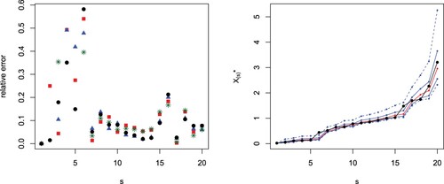12) ), the predictions with unknown parameter ϑ are obtained. In Figure 1 (left), we plot the difference in absolute value between exact values and predictions based on the median and the mean assuming both known and unknown value of the parameter. Note that with unknown ϑ some predictions based on the median and on the mean are not given in the figure in order to preserve its readability. We observe that, under the assumption of known ϑ, the predictions based on the median are better than the predictions based on the mean in 10 over 19 cases, while in one case (r = 19) they give the same value. Similarly, with unknown ϑ, the predictions based on the median are better than the predictions based on the mean in 11 over 19 cases and they are equal for r = 19.

Figure 1. Absolute value differences between generalized order statistics and predictions with known parameter ϑ based on the median (black circles) or the mean (red squares) and with unknown parameter ϑ based on the median (blue triangles) or the mean (green stars) from the simulated sample in Example 5.1 with m = 20, and s−r = 1 (left). Predictions (red) for $X_{(s)}^{\ast }$ from $X_{(r)}^{\ast }$ for m = 20, s−r = 1, for the exponential distribution in Example 5.1. The black points are the observed values and the blue lines are the limits for the $50\mathrm{\%}$ (continuous lines) and the $90\mathrm{\%}$ (dashed lines) prediction intervals (right).

Similarly, by replacing the median $q_{0.5}$ with $q_{0.25}$, $q_{0.75}$, $q_{0.05}$ and $q_{0.95}$ we obtain the 50% and $90\mathrm{\%}$ quantile prediction intervals. The results are plotted in Figure 1 (right). There we can observe that 2-out-of-19 exact points do not belong to the $90\mathrm{\%}$ prediction interval and 8-out-of-19 do not belong to the $50\mathrm{\%}$ prediction interval.

Now, we turn on considering the case s = r + 2. In this case, under the parameter and the model assumptions, the predictions and the prediction intervals are obtained by the quantiles of $G_2(u;{\gamma }_{r+1},{\gamma }_{r+2})={\gamma }_{r+1}{u}^{{\gamma }_{r+1}-1}-{\gamma }_{r+2}{u}^{{\gamma }_{r+2}-1}.$By analogy, we can obtain point predictions based on the mean by using ${\tilde{X}}_{(r+2)}^{\ast }=m_{\mathrm{mean}}(X_{(r)}^{\ast })=X_{(r)}^{\ast }-\frac{1}{\vartheta }\log \left(\frac{{\gamma }_{r+1}}{1+{\gamma }_{r+1}}\right)-\frac{1}{\vartheta }\log \left(\frac{{\gamma }_{r+2}}{1+{\gamma }_{r+2}}\right).$By analogy with the case s = r + 1, predictions with unknown ϑ can be obtained as well. 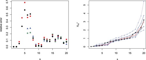In Figure 2 (left) we plot the difference in absolute value between exact values and predictions obtained with the median and the mean assuming both known and unknown value of the parameter, by leaving out the predictions with unknown ϑ for $r=1,2$ and 3 as they are much bigger compared to the others. In the figure, we can observe that the predictions based on the median are better than the ones based on the mean in 15 over 18 cases assuming known ϑ, while they are better in 9 over 18 cases and equal for r = 17 assuming unknown ϑ.

Figure 2. Absolute value differences between generalized order statistics and predictions with known parameter ϑ based on the median (black circles) or the mean (red squares) and with unknown parameter ϑ based on the median (blue triangles) or the mean (green stars) from the simulated sample in Example 5.1 with m = 20, and s−r = 2 (left). Predictions (red) for $X_{(s)}^{\ast }$ from $X_{(r)}^{\ast }$ for m = 20, s−r = 2, for the exponential distribution in Example 5.1. The black points are the observed values and the blue lines are the limits for the $50\mathrm{\%}$ (continuous lines) and the $90\mathrm{\%}$ (dashed lines) prediction intervals (right).

In Figure 2 (right), we plot the predictions for $X_{(s)}^{\ast }$ (red line), s = r + 2 jointly with the limits of the $90\mathrm{\%}$ (dashed blue lines) and $50\mathrm{\%}$ (continuous blue line) prediction intervals in the simulated sample. In this case, we can observe that 2-out-of-18 exact points do not belong to the $90\mathrm{\%}$ prediction interval and 8-out-of-18 do not belong to the $50\mathrm{\%}$ prediction interval.

As the parameters ${\gamma }_1,\dots ,{\gamma }_m$ are all different, it is possible to use (4(4) $\begin{array}{rl}{F}_{\ast ,r,s}^{({\gamma }_{r+1},\dots ,{\gamma }_s)}(t)& =1-(-1{)}^{s-r-1}\left(\prod _{j=r+1}^s{\gamma }_j\right)\sum _{j=r+1}^s{\gamma }_j^{-1}(\prod _{\begin{array}{c}k=r+1\\ v\ne j\end{array}}^s({\gamma }_j-{\gamma }_k{)}^{-1}){\mathrm{e}}^{-{\gamma }_{j}t},\\ & t\ge 0.\end{array}$(4) ) to determine the predictions and the prediction bands for the cases in which $s-r\ge 2$. Assuming known ϑ, the results are presented for some selected choices of r and s in Table 1. Then, in Table 2, we present the number of exact values which do not belong to the 50% and $90\mathrm{\%}$ prediction intervals. We obtain also the point predictions based on the mean with known ϑ and on the median and the mean with unknown ϑ, and the results are given in Tables 3–5, respectively. From the tables, we can observe that the predictions based on both the median and the mean assuming unknown ϑ are really bad for small values of r, while they are comparable with the predictions assuming known ϑ for higher values of r.

Table 1. Predicted values based on the median ${\hat{X}}_{(s)}^{\ast }$ from $X_{(r)}^{\ast }$ assuming known ϑ in Example 5.1 for some choices of r and s such that $s-r\ge 2$. In the bottom line we provide the exact values.

	s
r	3	6	9	11	14	18	20
1	0.10948	0.29518	0.52390	0.71184	1.08320	1.99725	3.34785
2		0.27948	0.50814	0.69607	1.06741	1.98148	3.33210
5			0.41177	0.59962	0.97092	1.88498	3.23571
7			0.65108	0.83860	1.20979	2.12384	3.47464
10					1.22134	2.13525	3.48622
12					1.08445	1.99768	3.34884
15						1.71923	3.07052
$X_{(s)}^{\ast }$	0.11512	0.44063	0.65636	0.81377	1.00213	1.74417	3.20779

Table 2. Number of exact values out of the 50% and $90\mathrm{\%}$ prediction intervals with fixed r in the sample of size 20 considered in Example 5.1.

r	1	2	3	4	5	6	7	8	9	10	11	12	13	14	15	16	17	18
$50\mathrm{\%}$	5	6	6	6	5	4	3	5	3	5	3	1	1	0	1	1	0	0
$90\mathrm{\%}$	0	0	0	1	2	0	0	1	0	1	0	0	0	0	0	0	0	0
out-of	18	17	16	15	14	13	12	11	10	9	8	7	6	5	4	3	2	1

Table 3. Predicted values based on the mean ${\tilde{X}}_{(s)}^{\ast }$ from $X_{(r)}^{\ast }$ assuming known ϑ in Example 5.1 for some choices of r and s such that $s-r\ge 2$. In the bottom line we provide the exact values.

	s
r	3	6	9	11	14	18	20
1	0.12407	0.30639	0.52953	0.71186	1.06853	1.91583	3.01444
2		0.29241	0.51555	0.69787	1.05455	1.90185	3.00046
5			0.42581	0.60813	0.96481	1.81211	2.91072
7			0.67079	0.85312	1.20979	2.05709	3.15570
10					1.23466	2.08196	3.18057
12					1.11120	1.95850	3.05711
15						1.71921	2.81782
$X_{(s)}^{\ast }$	0.11512	0.44063	0.65636	0.81377	1.00213	1.74417	3.20779

Table 4. Predicted values based on the median ${\hat{X}}_{(s)}^{\ast }$ from $X_{(r)}^{\ast }$ assuming unknown ϑ in Example 5.1 for some choices of r and s such that $s-r\ge 2$. In the bottom line we provide the exact values.

	s
r	3	6	9	11	14	18	20
1	0.26130	0.75758	1.36886	1.87115	2.86363	5.30647	8.91601
2		0.46867	0.89091	1.23794	1.92367	3.61162	6.10569
5			0.68207	1.51595	1.79355	3.61050	6.29546
7			0.63285	0.79429	1.11440	1.90267	3.06785
10					1.17024	1.97769	3.17129
12					1.08362	1.99348	3.33965
15						1.81067	3.34024
$X_{(s)}^{\ast }$	0.11512	0.44063	0.65636	0.81377	1.00213	1.74417	3.20779

Table 5. Predicted values based on the mean ${\tilde{X}}_{(s)}^{\ast }$ from $X_{(r)}^{\ast }$ assuming unknown ϑ in Example 5.1 for some choices of r and s such that $s-r\ge 2$. In the bottom line we provide the exact values.

	s
r	3	6	9	11	14	18	20
1	0.30029	0.78755	1.38392	1.87118	2.82442	5.08887	8.02497
2		0.49254	0.90460	1.24128	1.89992	3.46456	5.49328
5			0.70998	1.07240	1.78139	3.46564	5.64945
7			0.64958	0.80681	1.11440	1.84510	2.79253
10					1.18201	1.93061	2.90124
12					1.11027	1.95444	3.04900
15						1.81065	3.05419
$X_{(s)}^{\ast }$	0.11512	0.44063	0.65636	0.81377	1.00213	1.74417	3.20779

In the following example, we study the performance of our predictions for a different model of generalized order statistics in a sample with parent exponential distribution.

Example 5.2

Now, by analogy with Example 5.1, we consider again a standard exponential distribution and a sample of size m = 20, but with parameters ${\gamma }_1,\dots ,{\gamma }_m$ defined by ${\gamma }_j=1+3(m-j)$, that is, we consider 2-generalized order statistics with parameter k = 1 (see Cramer [16, p. 5]). The simulated generalized order statistics $X_{(1)}^{\ast },\dots ,X_{(m)}^{\ast }$, are given by $\overline{)\begin{array}{cccccccccc}0.00645& 0.01934& 0.03980& 0.03990& 0.04780& 0.15333& 0.17993& 0.22750& 0.22902& 0.27385\\ 0.28495& 0.30155& 0.32629& 0.35364& 0.36261& 0.53678& 0.62394& 0.64424& 0.90502& 1.84707\end{array}}$By proceeding as described in Example 5.1, we obtain the median and the mean predictions for $X_{(2)}^{\ast },\dots ,$ $X_{(m)}^{\ast }$ 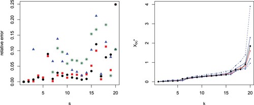both in the case of known and unknown parameter ϑ. In Figure 3 (left) we plot the difference in absolute value between exact values and predictions based on the median or the mean assuming known and unknown value of ϑ. There we observe that, assuming known ϑ, the predictions based on the median are better than the predictions based on the mean in 10 over 19 cases, while in one case (r = 19) they give the same value. Similarly, assuming unknown ϑ, the predictions based on the median are better than the predictions based on the mean in 12 over 19 cases and they are equal for r = 19. In this case, the predictions based on the assumption of known ϑ perform much better than the predictions based on unknown ϑ (as expected). Furthermore, we obtain the 50% and $90\mathrm{\%}$ quantile prediction intervals. The results are plotted in Figure 3 (right). There we can observe that 2-out-of-19 exact points do not belong to the $90\mathrm{\%}$ prediction interval and 8-out-of-19 do not belong to the $50\mathrm{\%}$ prediction interval.

Figure 3. Absolute value differences between generalized order statistics and predictions with known parameter ϑ based on the median (black circles) or the mean (red squares) and with unknown parameter ϑ based on the median (blue triangles) or the mean (green stars) from the simulated sample in Example 5.2 with m = 20, and s−r = 1 (left). Predictions (red) for $X_{(s)}^{\ast }$ from $X_{(r)}^{\ast }$ for m = 20, s−r = 1, for the exponential distribution in Example 5.2. The black points are the observed values and the blue lines are the limits for the $50\mathrm{\%}$ (continuous lines) and the $90\mathrm{\%}$ (dashed lines) prediction intervals (right).

In the case s = r + 2, with the parameters and the model assumptions stated above, the predictions and the prediction intervals are obtained by the quantiles of $G_2(u;{\gamma }_{r+1},{\gamma }_{r+2})=(m-r-\frac{2}{3})u^{3m-3r-5}-(m-r-\frac{5}{3})u^{3m-3r-2}.$Analogously, we obtain the predictions based on the mean and the predictions with unknown ϑ.

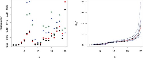
In Figure 4 (left) we plot the difference in absolute value between exact values and predictions based on the median or the mean both assuming known and unknown parameter ϑ. There, we can observe that, assuming known ϑ, the predictions based on the median are better than the ones based on the mean in 15 over 18 cases. In the case of unknown parameter ϑ, the predictions based on the median are better than the ones based on the mean in 11 over 18 cases. In Figure 4 (right), we plot the predictions for $X_{(s)}^{\ast }$ (red line), s = r + 2 jointly with the limits of the $90\mathrm{\%}$ (dashed blue lines) and $50\mathrm{\%}$ (continuous blue line) prediction intervals in the simulated sample. In this case, we can observe that 2-out-of-18 exact points do not belong to the $90\mathrm{\%}$ prediction interval and 8-out-of-18 do not belong to the $50\mathrm{\%}$ prediction interval.

Figure 4. Absolute value differences between generalized order statistics and predictions with known parameter ϑ based on the median (black circles) or the mean (red squares) and with unknown parameter ϑ based on the median (blue triangles) or the mean (green stars) from the simulated sample in Example 5.2 with m = 20, and s−r = 2 (left). Predictions (red) for $X_{(s)}^{\ast }$ from $X_{(r)}^{\ast }$ for m = 20, s−r = 2, for the exponential distribution in Example 5.2. The black points are the observed values and the blue lines are the limits for the $50\mathrm{\%}$ (continuous lines) and the $90\mathrm{\%}$ (dashed lines) prediction intervals (right).

As the parameters ${\gamma }_1,\dots ,{\gamma }_m$ are all different, it is possible to use (4(4) $\begin{array}{rl}{F}_{\ast ,r,s}^{({\gamma }_{r+1},\dots ,{\gamma }_s)}(t)& =1-(-1{)}^{s-r-1}\left(\prod _{j=r+1}^s{\gamma }_j\right)\sum _{j=r+1}^s{\gamma }_j^{-1}(\prod _{\begin{array}{c}k=r+1\\ v\ne j\end{array}}^s({\gamma }_j-{\gamma }_k{)}^{-1}){\mathrm{e}}^{-{\gamma }_{j}t},\\ & t\ge 0.\end{array}$(4) ) to determine the predictions and the prediction bands for the cases in which $s-r\ge 2$. In Table 6 the results are presented for some selected choices of r and s assuming known ϑ. In Table 7, we present the number of exact values which do not belong to the 50% and $90\mathrm{\%}$ prediction intervals. We obtain also the point predictions based on the mean with known ϑ and on the median and the mean with unknown ϑ, and the results are given in Tables 8–10. From the tables, we can observe that the predictions based on both the median and the mean assuming unknown ϑ are really bad for small values of r, while they are comparable with the predictions assuming known ϑ for higher values of r, and on average even better in the case of the predictions based on the mean.

Table 6. Predicted values based on the median ${\hat{X}}_{(s)}^{\ast }$ from $X_{(r)}^{\ast }$ assuming known ϑ in Example 5.2 for some choices of r and s such that $s-r\ge 2$. In the bottom line we provide the exact values.

	s
r	3	6	9	11	14	18	20
1	0.03784	0.10242	0.18274	0.24962	0.38469	0.74947	1.76574
2		0.09698	0.17730	0.24419	0.37921	0.74401	1.76033
5			0.14382	0.21063	0.34566	0.71052	1.72696
7			0.22727	0.29398	0.42898	0.79377	1.81041
10					0.43295	0.79774	1.81470
12					0.38377	0.74831	1.76561
15						0.64459	1.66292
$X_{(s)}^{\ast }$	0.03980	0.15333	0.22902	0.28495	0.35364	0.64422	1.84707

Table 7. Number of exact values out of the 50% and $90\mathrm{\%}$ prediction intervals with fixed r in the sample of size 20 considered in Example 5.2.

r	1	2	3	4	5	6	7	8	9	10	11	12	13	14	15	16	17	18
$50\mathrm{\%}$	6	6	7	6	5	4	4	5	3	5	3	1	1	0	1	1	0	0
$90\mathrm{\%}$	0	0	0	1	2	0	0	1	0	1	0	0	0	0	0	0	0	0
out-of	18	17	16	15	14	13	12	11	10	9	8	7	6	5	4	3	2	1

Table 8. Predicted values based on the mean ${\tilde{X}}_{(s)}^{\ast }$ from $X_{(r)}^{\ast }$ assuming known ϑ in Example 5.2 for some choices of r and s such that $s-r\ge 2$. In the bottom line we provide the exact values.

	s
r	3	6	9	11	14	18	20
1	0.04352	0.10822	0.18856	0.25540	0.39037	0.75394	1.67024
2		0.10309	0.18344	0.25028	0.38524	0.74882	1.66511
5			0.15114	0.21798	0.35295	0.71652	1.63281
7			0.23559	0.30243	0.43739	0.80097	1.71726
10					0.44391	0.80748	1.72377
12					0.39730	0.76087	1.67716
15						0.66556	1.58185
$X_{(s)}^{\ast }$	0.03980	0.15333	0.22902	0.28495	0.35364	0.64422	1.84707

Table 9. Predicted values based on the median ${\hat{X}}_{(s)}^{\ast }$ from $X_{(r)}^{\ast }$ assuming unknown ϑ in Example 5.2 for some choices of r and s such that $s-r\ge 2$. In the bottom line we provide the exact values.

	s
r	3	6	9	11	14	18	20
1	0.09034	0.26294	0.47758	0.65532	1.01731	1.99221	4.70826
2		0.16271	0.31103	0.43456	0.68389	1.35753	3.23429
5			0.23866	0.37148	0.63988	1.36515	3.38562
7			0.22076	0.27829	0.39471	0.70930	1.58603
10					0.41442	0.73671	1.63520
12					0.38346	0.74667	1.76021
15						0.68179	1.83447
$X_{(s)}^{\ast }$	0.03980	0.15333	0.22902	0.28495	0.35364	0.64422	1.84707

Table 10. Predicted values based on the mean ${\tilde{X}}_{(s)}^{\ast }$ from $X_{(r)}^{\ast }$ assuming unknown ϑ in Example 5.2 for some choices of r and s such that $s-r\ge 2$. In the bottom line we provide the exact values.

	s
r	3	6	9	11	14	18	20
1	0.10551	0.27842	0.49316	0.67179	1.03250	2.00417	4.45301
2		0.17339	0.32236	0.44579	0.69502	1.36640	3.05845
5			0.25322	0.38608	0.65436	1.37707	3.19847
7			0.22793	0.28557	0.40196	0.71550	1.50570
10					0.42410	0.74532	1.55487
12					0.39695	0.75918	1.67209
15						0.70552	1.74270
$X_{(s)}^{\ast }$	0.03980	0.15333	0.22902	0.28495	0.35364	0.64422	1.84707

In the last example, we discuss again the model used in Example 5.2 and analyze the coverage of the 50% and $90\mathrm{\%}$ prediction intervals.

Example 5.3

Consider the model already presented in Example 5.2, i.e., standard exponential distribution and a sample of size m = 20, with parameters ${\gamma }_1,\dots ,{\gamma }_m$ defined by ${\gamma }_j=1+3(m-j)$. To better analyze the predictions, we simulate N = 100 random samples of size m. Then, by fixing the values of r and s, we get the predictions for each sample. We start with the case s = r + 1 and in particular with r = 4 and s = 5. The results are plotted in Figure 5 (left). There, we can observe that 49 values do not belong to the $50\mathrm{\%}$ prediction intervals and 14 values do not belong to the $90\mathrm{\%}$ prediction intervals. Now, we consider the case s = r + 2, with r = 4 and s = 6. 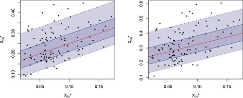The results are plotted in Figure 5 (right) where we can observe that 54 and 13 values do not belong to the 50% and $90\mathrm{\%}$ prediction intervals, respectively. In Figure 6, we consider some cases in which the difference s−r is greater than two. More precisely, in Figure 6 (left) we have r = 4 and s = 10 with 59 and 15 values out of the 50% and $90\mathrm{\%}$ prediction intervals, respectively, and in Figure 6 (right) we have r = 4 and s = 12 with 56 and 15 values out of the 50% and $90\mathrm{\%}$ prediction intervals, respectively.

Figure 5. Scatterplots of a simulated sample of size N = 100 from $(X_{(r)}^{\ast },X_{(s)}^{\ast })$ for $m=20$, r = 4 and s = 5 (left) and r = 4, s = 6 (right) for the exponential distribution in Example 5.3 jointly with the theoretical median regression curves (red) and $50\mathrm{\%}$ (dark grey) and $90\mathrm{\%}$ (light grey) prediction bands.

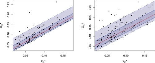
Figure 6. Scatterplots of a simulated sample of size N = 100 from $(X_{(r)}^{\ast },X_{(s)}^{\ast })$ for $m=20$, r = 4 and s = 10 (left) and r = 4, s = 12 (right) for the exponential distribution in Example 5.3 jointly with the theoretical median regression curves (red) and $50\mathrm{\%}$ (dark grey) and $90\mathrm{\%}$ (light grey) prediction bands.

6. Conclusion and outlook

In this paper, we have provided different tools to predict future data from present and past data in ordered data sets that can be modelled as generalized order statistics. These results extend preceding ones for order statistics and record values (that are included in the generalized order statistics' model as particular cases). The quantile regression technique allows us to provide not only point predictions but also confidence regions for those values.

The examples included in Section 5 show how to apply the established theoretical results to specific situations with different assumptions and tools. In the first example, we consider ordered data from a sample (of order statistics) with a baseline exponential distribution and we use mean and median predicted values, providing 50% and 90% confidence prediction bands as well. We do the same in the second example but with data from a 2-generalized order statistics' model. The coverage probabilities for the quantile regression bands obtained with this model are analyzed in the third example. These techniques can be used to analyze similar examples with ordered data.

There are several tasks for future research projects. As already mentioned above, we can study different models and/or different baseline distributions (Weibull, Pareto, etc.). Especially, the case of unknown parameters is of particular interest. So far, the regression approach is based on a completely known baseline distribution function F. However, one may consider estimators of the cumulative distribution function F and the quantile function $F^{\leftarrow }$. For instance, suppose $F_{\vartheta }$ is the cumulative distribution function of an $\mathsf{\text{Exp}}(\vartheta )$-distribution with unknown mean $\vartheta >0$. Given an estimator $\hat{\vartheta }$ of ϑ, one can estimate $F_{\vartheta }$ and $F_{\vartheta }^{\leftarrow }$ by the corresponding plug-in estimators. Then, from (11(11) $m_{\mathrm{mean}}(x)={\overline{F}}^{\leftarrow }(\overline{F}(x)\prod _{j=r+1}^s\frac{{\gamma }_j}{1+{\gamma }_j}).$(11) ), we get the predictor ${\hat{m}}_{\mathrm{mean}}(x)={\overline{F}}_{\hat{\vartheta }}^{\leftarrow }({\overline{F}}_{\hat{\vartheta }}(x)\prod _{j=r+1}^s\frac{{\gamma }_j}{1+{\gamma }_j})=x-\frac{1}{\hat{\vartheta }}\ln \left(\prod _{j=r+1}^s\frac{{\gamma }_j}{1+{\gamma }_j}\right),$which has the same form as the maximum likelihood predictor given in (15(15) ${\hat{X}}_{(s)}^{\ast }=X_{(r)}^{\ast }+m_{{\gamma }_{r+1},\dots ,{\gamma }_s}/{\hat{\vartheta }}_{\mathrm{MLE}}.$(15) ). However, its computation does not involve any computational method. Hence, we get for a generalized order statistics' model alternative but always explicit predictors to those obtained in Section 4.2 for an unknown mean. In particular, for order statistics and record values, we find the predictors ${\hat{m}}_{\mathrm{mean}}(x)=x-\frac{1}{\hat{\vartheta }}\ln \left(\frac{n-s+1}{n-r+1}\right),{\hat{m}}_{\mathrm{mean}}(x)=x+\frac{s-r}{\hat{\vartheta }}\ln (2).$Similarly, the other regression methods can be taken into account. Furthermore, if $\hat{\vartheta }$ is a consistent estimator of the mean ϑ, asymptotic confidence bands can be obtained in such a situation. It would be interesting to study these predictors and extend the method to other distributions. Another relevant task is to develop fit tests to determine whether our techniques can be applied for given data. All these problems are crucial in order to provide accurate predictions for future data values. Finally, one may consider Type-I or hybrid censored data (see Balakrishnan et al. [40] for a recent review of these models and related results) and apply the regression approach to predictions based on this kind of data.

Acknowledgements

The authors are grateful to an associate editor and two reviewers for suggestions which led to an improved version of the manuscript.

Disclosure statement

No potential conflict of interest was reported by the author(s).

Additional information

Funding

Francesco Buono is member of the research group GNAMPA of INdAM (Istituto Nazionale di Alta Matematica). Jorge Navarro thanks the support of Ministerio de Ciencia e Innovación of Spain AEI/10.13039/501100011033 under grants PID2019-103971GB-I00 and PID2022-137396NB-I00.

References

- David HA, Nagaraja HN. Order statistics. 3rd ed. Hoboken (NJ): Wiley; 2003.
- Arnold BC, Balakrishnan N, Nagaraja HN. A first course in order statistics. Philadelphia: Society for Industrial and Applied Mathematics (SIAM); 2008.
- Hahn GJ, Meeker WQ, Escobar LA. Statistical intervals: a guide for practitioners. New York: Wiley; 2017.
- Balakrishnan N, Cramer E. The art of progressive censoring. applications to reliability and quality. New York: Birkhäuser; 2014.
- Navarro J. Prediction of record values by using quantile regression curves and distortion functions. Metrika. 2021;85:675–706. doi: 10.1007/s00184-021-00847-w
- Navarro J, Buono F. Predicting future failure times by using quantile regression. Metrika. 2023;86:543–576. doi: 10.1007/s00184-022-00884-z
- Volovskiy G. Likelihood-based prediction in models of ordered data [PhD thesis]. RWTH Aachen, Aachen; 2018.
- Volovskiy G, Kamps U. Maximum observed likelihood prediction of future record values. TEST. 2020;29:1072–1097. doi: 10.1007/s11749-020-00701-7
- Kamps U. A concept of generalized order statistics. Stuttgart: Teubner; 1995.
- Cramer E, Kamps U. Marginal distributions of sequential and generalized order statistics. Metrika. 2003;58:293–310. doi: 10.1007/s001840300268
- Kaminsky KS, Rhodin L. Maximum likelihood prediction. Ann Inst Stat Math. 1985;37:507–517. doi: 10.1007/BF02481119
- Cramer E, Kamps U. Sequential k-out-of-n systems. In: Balakrishnan N, Rao CR, editors. Handbook of statistics: advances in reliability. Vol. 20, Chapter 12. Amsterdam: Elsevier; 2001. p. 301–372.
- Malmquist S. On a property of order statistics from a rectangular distribution. Skand Aktuarietidskr. 1950;33:214–222.
- Cramer E. Sequential order statistics. In: Kotz S, Balakrishnan N, Read CB, Vidakovic B, Johnson NL, editors. Encyclopedia of statistical sciences. Update Vol. 12. Hoboken (NJ): Wiley; 2006. p. 7629–7634.
- Rao CR. On some problems arising out of discrimination with multiple characters. Sankhyā. 1949;9:343–366.
- Cramer E. Contributions to generalized order statistics. Oldenburg, Germany: Habilitationsschrift, University of Oldenburg; 2003.
- Bdair OM, Raqab MZ. Prediction of future censored lifetimes from mixture exponential distribution. Metrika. 2022;85:833–857. doi: 10.1007/s00184-021-00852-z
- Kamps U, Cramer E. On distributions of generalized order statistics. Statistics. 2001;35:269–280. doi: 10.1080/02331880108802736
- Springer MD, Thompson WE. The distribution of products of beta, gamma and Gaussian random variables. SIAM J Appl Math. 1970;18:721–737. doi: 10.1137/0118065
- Springer MD. The algebra of random variables. New York: Wiley; 1979.
- Botta RF, Harris CM, Marchal WG. Characterizations of generalized hyperexponential distribution functions. Comm Stat Stoch Models. 1987;3:115–148. doi: 10.1080/15326348708807049
- Mathai AM. A handbook of generalized special functions for statistical and physical sciences. Oxford: Clarendon Press; 1993.
- Akkouchi M. On the convolution of exponential distributions. J Chungcheong Math Soc. 2008;21:501–510.
- Levy E. On the density for sums of independent exponential, Erlang and gamma variates. Stat Papers. 2022;63:693–721. doi: 10.1007/s00362-021-01256-x
- Cramer E. Hermite interpolation polynomials and distributions of ordered data. Stat Methodol. 2009;6:337–343. doi: 10.1016/j.stamet.2008.12.004
- Cramer E. Logconcavity and unimodality of progressively censored order statistics. Stat Probab Lett. 2004;68:83–90. doi: 10.1016/j.spl.2004.01.016
- Cramer E, Kamps U, Rychlik T. Unimodality of uniform generalized order statistics, with applications to mean bounds. Ann Inst Stat Math. 2004;56:183–192. doi: 10.1007/BF02530531
- Cuculescu I, Theodorescu R. Multiplicative strong unimodality. Aust N Z J Stat. 1998;40:205–214. doi: 10.1111/anzs.1998.40.issue-2
- Cramer E. Dependence structure of generalized order statistics. Statistics. 2006;40:409–413. doi: 10.1080/02331880600822291
- Navarro J. Introduction to system reliability theory. Cham: Springer; 2021.
- Navarro J, Calı C, Longobardi M, et al. Distortion representations of multivariate distributions. Stat Methods Appl. 2022;31:925–954. doi: 10.1007/s10260-021-00613-2
- Bieniek M. Variation diminishing property of densities of uniform generalized order statistics. Metrika. 2007;65:297–309. doi: 10.1007/s00184-006-0077-4
- Cramer E, Kamps U. Estimation with sequential order statistics from exponential distributions. Ann Inst Stat Math. 2001;53:307–324. doi: 10.1023/A:1012470706224
- Hermanns M, Cramer E, Ng HKT. EM algorithms for ordered and censored system lifetime data under a proportional hazard rate model. J Stat Comput Simul. 2020;90:3301–3337. doi: 10.1080/00949655.2020.1800706
- Glen AG. Accurate estimation with one order statistic. Comput Stat Data Anal. 2010;54:1434–1441. doi: 10.1016/j.csda.2010.01.012
- Marshall AW, Olkin I. Life distributions. structure of nonparametric, semiparametric, and parametric families. New York (NY): Springer; 2007.
- Zografos K, Balakrishnan N. On families of beta- and generalized gamma-generated distributions and associated inference. Stat Methodol. 2009;6:344–362. doi: 10.1016/j.stamet.2008.12.003
- Cordeiro GM, Brito RS. The beta power distribution. Braz J Probab Stat. 2012;26:88–112. doi: 10.1214/10-bjps124
- Arnold BC, Balakrishnan N, Nagaraja HN. Records. New York: Wiley; 1998.
- Balakrishnan N, Cramer E, Kundu D. Hybrid censoring know-how – designs and implementations. Cambridge: Academic; 2023.