Inner approximation algorithm for solving linear multiobjective optimization problems

ABSTRACT

Benson's outer approximation algorithm and its variants are the most frequently used methods for solving linear multiobjective optimization problems. These algorithms have two intertwined parts: single-objective linear optimization on one hand, and a combinatorial part closely related to vertex enumeration on the other. Their separation provides a deeper insight into Benson's algorithm, and points toward a dual approach. Two skeletal algorithms are defined which focus on the combinatorial part. Using different single-objective optimization problems yields different algorithms, such as a sequential convex hull algorithm, another version of Benson's algorithm with the theoretically best possible iteration count, and the dual algorithm of Ehrgott et al. [A dual variant of Benson's ‘outer approximation algorithm’ for multiple objective linear programming. J Glob Optim. 2012;52:757–778]. The implemented version is well suited to handle highly degenerate problems where there are many linear dependencies among the constraints. On problems with 10 or more objectives, it shows a significant increase in efficiency compared to Bensolve – due to the reduced number of iterations and the improved combinatorial handling.

KEYWORDS:

• Multiobjective optimization
• duality
• vertex enumeration
• double description
• objective space

AMS CLASSIFICATION NUMBERS:

• 90C29
• 90C05

1. Introduction

Our notation is standard and mainly follows that of [1,2]. The transpose of the matrix M is denoted by $M^{\mathrm{T}}$. Vectors are usually denoted by small letters and are considered as single column matrices. For two vectors, x and y of the same dimension, xy denotes their inner product, which is the same as the matrix product $x^{\mathrm{T}}y$. The ith coordinate of x is denoted by $x_i$, and $x\le y$ means that for every coordinate i, $x_i\le y_i$. The non-negative orthant ${\mathbb{R}}_{\ge }^n$ is the collection of vectors $x\in {\mathbb{R}}^n$ with $x\ge 0$, that is, vectors whose coordinates are non-negative numbers.

For an introduction to higher-dimensional polytopes, see [3], and for a description of the double description method and its variants, consult [4]. Linear multiobjective optimization problems, methods, and algorithms are discussed in [1,5,6] and the references therein.

1.1. The MOLP problem

Given positive integers n, m, and p, the $m\times n$ matrix A maps the problem space ${\mathbb{R}}^n$ to ${\mathbb{R}}^m$, and the $p\times n$ matrix P maps the problem space ${\mathbb{R}}^n$ to the objective space ${\mathbb{R}}^p$. For better clarity, we use x to denote points of the problem space ${\mathbb{R}}^n$, while y denotes points in the objective space ${\mathbb{R}}^p$. In the problem space, a convex closed polyhedral set $\mathcal{A}$ is specified by a collection of linear constraints. For simplicity, we assume that the constraints are given in the following special format. This format will only be used in Section 5. (1) $\mathcal{A}=\{x\in {\mathbb{R}}^n:Ax=c,x\ge 0\},$(1) where $c\in {\mathbb{R}}^m$ is a fixed vector. The p-dimensional linear projection of $\mathcal{A}$ given by the $p\times n$ matrix P is (2) $\mathcal{Q}=P\mathcal{A}=\{Px:x\in \mathcal{A}\}.$(2) Using this notation, the multiobjective linear optimization problem can be cast as follows: MOLP $\text{find}\underset{y}{min}\{y:y\in \mathcal{Q}\},$MOLP where minimization is understood with respect to the coordinate-wise ordering of ${\mathbb{R}}^p$. The point $\hat{y}\in \mathcal{Q}$ is non-dominated or Pareto optimal, if no $y\le \hat{y}$ different from $\hat{y}$ is in $\mathcal{Q}$; and it is weakly non-dominated if no $y<\hat{y}$ is in $\mathcal{Q}$. Solving the multiobjective optimization problem is to find (a description of) all non-dominated vectors $\hat{y}$ together with corresponding pre-images $\hat{x}\in {\mathbb{R}}^n$ such that $\hat{y}=P\hat{x}$.

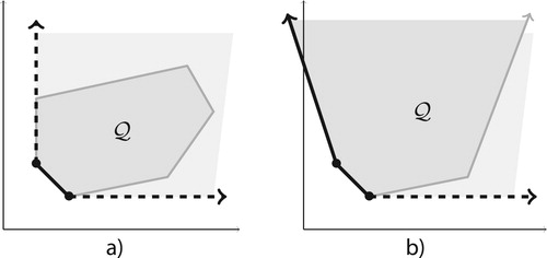
Let ${\mathcal{Q}}^{+}=\mathcal{Q}+{\mathbb{R}}_{\ge }^p$, the Minkowski sum of $\mathcal{Q}$ and the non-negative orthant of ${\mathbb{R}}^p$, see [3]. It follows easily from the definitions, but see also [1,7,8], that non-dominated points of $\mathcal{Q}$ and of ${\mathcal{Q}}^{+}$ are the same. The weakly non-dominated points of ${\mathcal{Q}}^{+}$ form its Pareto front. Figure 1 illustrates non-dominated (solid line), and weakly non-dominated points (solid and dashed line) of ${\mathcal{Q}}^{+}$ when (a) all objectives are bounded from below, and when (b) the first objective is not bounded. ${\mathcal{Q}}^{+}$ is the unbounded light grey area extending $\mathcal{Q}$.

Figure 1. Pareto front with (a) bounded, (b) unbounded objectives.

1.2. Facial structure of polytopes

Let us recall some facts concerning the facial structure of n-dimensional convex closed polytopes. A face of such a polytope $\mathcal{B}\subset {\mathbb{R}}^n$ is the intersection of $\mathcal{B}$ and some closed halfspace (including the empty set and the whole $\mathcal{B}$). Faces of dimension zero, one, n−2, and n−1 are called vertex, edge, ridge, and facet, respectively.

An n-dimensional halfspace is specified as $H=\{x\in {\mathbb{R}}^n:xh\ge M\}$, where $h\in {\mathbb{R}}^n$ is a non-null vector (normal), and M is a scalar (intercept). The positive side of H is the open halfspace $\{x\in {\mathbb{R}}^n:xh>M\}$; the negative side is defined similarly. Each facet of $\mathcal{B}$ is identified with the halfspace which contains $\mathcal{B}$ and whose boundary intersects $\mathcal{B}$ in that facet. $\mathcal{B}$ is just the intersection of all halfspaces corresponding to its facets.

The halfspace H is supporting if it contains $\mathcal{B}$, and there is a boundary point of $\mathcal{B}$ on the boundary of H. The boundary hyperplane of a supporting halfspace intersects $\mathcal{B}$ in one of its faces. All boundary points of $\mathcal{B}$ are in the relative interior of exactly one face.

A recession direction, or ray of $\mathcal{B}$ is a vector $d\in {\mathbb{R}}^n$ such that for some $x\in \mathcal{B}$, $x+\lambda d\in \mathcal{B}$ for all real $\lambda \ge 0$. d is extreme if whenever $d=d_1+d_2$ for two recession directions $d_1$ and $d_2$, then both $d_1$ and $d_2$ are non-negative multiples of d.

1.3. Working with unbounded polytopes

When $\mathcal{B}$ is unbounded but does not contain a complete line – which will always be the case in this paper – Burton and Ozlen's ‘oriented projective geometry’ can be used [9]. Intuitively this means that rays are represented by ideal points, extreme rays are the ideal vertices which lie on a single ideal facet determining the ideal hyperplane. Notions of ordering and convexity can be extended to these objects seamlessly even from a computational point of view. In particular, all non-ideal points are on the positive side of the ideal hyperplane. Thus in theoretical considerations, without loss of generality, $\mathcal{B}$ can be assumed to be bounded.

1.4. Assumptions on the MOLP problem

In order that we could focus on the main points, we make some simplifying assumptions on the (MOLP) to be solved. The main restriction is that all objectives are bounded from below. From this, it follows immediately that neither $\mathcal{Q}$ nor ${\mathcal{Q}}^{+}$ contains a complete line; and that the Pareto optimal solutions are the bounded faces of dimension p−1 and less of ${\mathcal{Q}}^{+}$ as indicated on Figure 1(a). One can relax this restriction at the expense of computing the extreme rays of $\mathcal{Q}$ first (also checking that ${\mathcal{Q}}^{+}$ does not contain a complete line), as is done by the software package Bensolve [10]. Further discussions are postponed to Section 6, where we also extend our results to the case where the ordering is given by some cone different from ${\mathbb{R}}_{\ge }^p$.

Assumption

The optimization problem (MOLP) satisfies the following conditions:

1. the n-dimensional polytope $\mathcal{A}$ defined in (1(1) $\mathcal{A}=\{x\in {\mathbb{R}}^n:Ax=c,x\ge 0\},$(1) ) is not empty;

2. each objective in $\mathcal{Q}$ is bounded from below.

An immediate consequence of the first assumption is that the projection $\mathcal{Q}=P\mathcal{A}$ is non-empty either, and then ${\mathcal{Q}}^{+}=\mathcal{Q}+{\mathbb{R}}_{\ge }^p$ is full-dimensional. According to Assumption 2, $\mathcal{Q}$ and ${\mathcal{Q}}^{+}$ is contained in $y+{\mathbb{R}}_{\ge }^p$ for some (real) vector $y\in {\mathbb{R}}^p$. Thus ${\mathcal{Q}}^{+}$ has exactly p ideal vertices, namely the positive endpoints of the coordinate axes, and these ideal vertices lie on the single ideal facet of ${\mathcal{Q}}^{+}$.

1.5. Benson's algorithm revisited

The solution of the (MOLP) can be recovered from a description of the Pareto front of ${\mathcal{Q}}^{+}$, which, in turn, is specified by the list of its vertices and (non-ideal) facets. Indeed, the set of Pareto optimal points is the union of those faces of ${\mathcal{Q}}^{+},$ which do not contain ideal points. Thus solving (MOLP) means find all vertices and facets of the polyhedron ${\mathcal{Q}}^{+}$.

Benson's ‘outer approximation algorithm’ and its variants [1,2,5–8,10] do exactly this, working in the (low-dimensional) objective space. These algorithms have two intertwined parts: scalar optimization on one hand, and a combinatorial part on the other. Their separation provides a deeper insight into how these algorithms work.

Benson's algorithm works in stages by maintaining a ‘double description’ of an approximation of the final polytope ${\mathcal{Q}}^{+}$. A convex polytope is uniquely determined as the convex hull of a finite set of points (for example, the set of vertices) and directions (in our case: ideal points) as well as the intersection of finitely many closed halfspaces (for example, halfspaces corresponding to the facets plus the ideal facet). The ‘double description’ refers to the technique keeping and maintaining both lists simultaneously. The iterative algorithm stops when the last approximation equals ${\mathcal{Q}}^{+}$. At this stage, both the vertices and facets of ${\mathcal{Q}}^{+}$ are computed, thus the (MOLP) has been solved.

During the algorithm, a new facet is added to the approximating polytope in each iteration. The new facet is determined by solving a smartly chosen scalar LP problem (specified from the description of the actual approximation). Then, the combinatorial step is executed: the new facet is merged to the approximation by updating the facet and vertex lists. This step is very similar to that of incremental vertex enumeration [4,11–13], and can be parallelized.

Section 2 defines two types of black box algorithms which, on each call, provide data for the combinatorial part. The point separating oracle separates a point from the (implicitly defined) polytope ${\mathcal{Q}}^{+}$ by a halfspace. The plane separating oracle is its dual: the input is a halfspace, and the oracle provides a point of ${\mathcal{Q}}^{+}$ on the negative side of that halfspace.

Two general enumeration algorithms are specified in Section 3 which call these black box algorithms repeatedly. It is proved that they terminate with a description of their corresponding target polytopes. Choosing the initial polytope and the oracle in some specific way, one gets a convex hull algorithm, a (variant of) Benson's algorithm, and the Ehrgott–Löhne–Shao dual algorithm.

Aspects of the combinatorial part are discussed in Section 4. Section 5 explains how the oracles in these algorithms can be realized. Finally, Section 6 discusses other implementation details, limitations and possible generalizations.

1.6. Our contribution

The first skeletal algorithm in Section 3.1 is the abstract versions of Benson's outer approximation algorithm and its variants, where the combinatorial part (vertex enumeration) and the scalar LP part has been separated. The latter one is modelled as an inquiry to a separating oracle which, on each call, provides the data the combinatorial part can work on. Using one of the point separation oracles in Section 5.1, one can recover, e.g. Algorithm 1 of [1]. The running time estimate in Theorem 3.4 is the same (with the same proof) as the estimate in [1, Theorem 4.6].

The other skeletal algorithm is the dual of the outer approximation one. The ‘inner’ algorithm of this paper uses the plane separation oracle defined in Section 5.3. Another instance is Algorithm 2 of Ehrgott et al. [1], called ‘dual variant of Benson's outer approximation algorithm’.

Studying these skeletal algorithms made it possible to clarify the role of the initial approximation, and prove general terminating conditions. While not every separating oracle guarantees termination, it is not clear what are the (interesting and realizable) sufficient conditions. Benson's outer approximation algorithm is recovered by the first separation oracle defined in Section 5.1. Other two separation oracles have stronger termination guarantees, yielding the first version which is guaranteed to take only the theoretically minimal number of iterations. Oracles in Section 5.3 are particularly efficient and contribute significantly to the excellent performance of the implemented inner approximation algorithm.

It is almost trivial to turn any of the skeletal algorithms to an incremental vertex (or facet) enumeration algorithm. Such algorithms have been studied extensively. Typically there is a blow-up in the size of the intermediate approximation; there are examples where even the last but one approximation has size $\mathrm{\Omega }\left(m^{\sqrt{p}/2}\right),$ where m is the final number of facets (or vertices) and p is the space dimension [14]. This blow-up can be significant when p is 6 or more.

An interesting extension to the usual single objective LP have been identified, where not one but several goals are specified, and called ‘multi-goal LP’. Optimization is done for the first goal, then within the solution space the second goal is optimized, that is, in the second optimization there is an additional constraint specifying that the first goal has an optimal value. Then within this solution space, the third goal is optimized, etc. Section 5.2 sketches how existing LP solvers can be patched to become an efficient multi-goal solver. We expect more interesting applications for this type of solvers.

2. Separating oracles

In this and in the following section, $\mathcal{B}\subset {\mathbb{R}}^p$ is some bounded, closed, convex polytope with non-empty interior. As discussed in Section 1.3, the condition that $\mathcal{B}$ is bounded can be replaced by the weaker assumption that $\mathcal{B}$ does not contain a complete line.

Definition 2.1

A point separating oracle $\mathsf{p}\mathsf{t}\mathsf{O}\left(\mathcal{B}\right)$ for the polytope $\mathcal{B}\subset {\mathbb{R}}^p$ is a black box algorithm with the following input/output behaviour:

1. a point $v\in {\mathbb{R}}^p$;

2. ‘inside’ if $v\in \mathcal{B}$; otherwise a halfspace H corresponding to a facet of $\mathcal{B}$ such that v is on the negative side of H.

Definition 2.2

A plane separating oracle $\mathsf{h}\mathsf{p}\mathsf{O}\left(\mathcal{B}\right)$ for the polytope $\mathcal{B}\subset {\mathbb{R}}^p$ is a black box algorithm with the following input/output behaviour:

1. a p-dimensional closed halfspace H;

2. ‘inside’ if $\mathcal{B}$ is a subset of H; otherwise a vertex v of $\mathcal{B}$ on the negative side of H.

The main point is that only the oracle uses the polytope $\mathcal{B}$ in the enumeration algorithms of Section 3, and $\mathcal{B}$ might not be defined by a collection of linear constraints. In particular, this happens when the algorithm is used to solve the multiobjective problem, where the polytope passed to the oracle is $\mathcal{Q}$ or ${\mathcal{Q}}^{+}$.

The two oracles are dual in the sense that if ${\mathcal{B}}^{\ast }$ is the geometric dual of the convex polytope $\mathcal{B}$ with the usual point versus hyperplane correspondence [3], then $\mathsf{p}\mathsf{t}\mathsf{O}\left(\mathcal{B}\right)$ and $\mathsf{h}\mathsf{p}\mathsf{O}\left({\mathcal{B}}^{\ast }\right)$ are equivalent: when a point is asked from oracle $\mathsf{p}\mathsf{t}\mathsf{O}\left(\mathcal{B}\right)$, ask the dual of this point from $\mathsf{h}\mathsf{p}\mathsf{O}\left({\mathcal{B}}^{\ast }\right)$, and return the dual of the answer.

The object returned by a weak separating oracle is not required to be a facet (or vertex), but only a supporting halfspace (or a boundary point) separating the input from the polytope. The returned separating object, however, cannot be arbitrary, it must have some structural property. Algorithms of Section 3 work with the weaker separating oracles defined below, but the performance guarantees are exponentially worse. On the other hand, such weak oracles can be realized easier. Actually, strong separating oracles in Section 5 are implemented as tweaked weak oracles.

Definition 2.3

A weak point separating oracle ${\mathsf{p}\mathsf{t}\mathsf{O}}^{\ast }(\mathcal{B}$) for the polytope $\mathcal{B}$ is a black box algorithm which works as follows. It fixes an internal point $o\in \mathcal{B}$.

1. a point $v\in {\mathbb{R}}^p$;

2. ‘inside’ if $v\in \mathcal{B}$; otherwise connect v to the fixed internal point o, compute where this line segment intersects the boundary of $\mathcal{B}$, and return a supporting halfspace H of $\mathcal{B}$ whose boundary touches $\mathcal{B}$ at that point (this H separates v and $\mathcal{B}$).

Definition 2.4

A weak plane separating oracle ${\mathsf{h}\mathsf{p}\mathsf{O}}^{\ast }\left(\mathcal{B}\right)$ for the polytope $\mathcal{B}$ is a black box algorithm which works as follows.

1. a halfspace H;

2. ‘inside’ if $\mathcal{B}$ is contained in H; otherwise a boundary point v of $\mathcal{B}$ on the negative side of H which is farthest away from the bounding hyperplane of H.

A strong oracle is not necessarily a weak one (for example, it can return any vertex on the negative side of H, not only the one which is farthest away from it), but can always give a response which is consistent with being a weak oracle. Similarly, there is always a valid response of a weak oracle which qualifies as correct answer for the corresponding strong oracle.

While strong oracles are clearly dual of each other, it is not clear whether the weak oracles are dual, and if yes, in what sense of duality.

3. Approximating algorithms

The skeletal algorithms below are called outer and inner approximations. The outer name reflects the fact that the algorithm approximates the target polytope from outside, while the inner does it from inside. The outer algorithm is an abstract version of Benson's algorithm where the computational and combinatorial parts are separated.

3.1. Skeletal algorithms

On input, both algorithms require two convex polytopes: $\mathcal{S}$ and $\mathcal{B}$. The polytope $\mathcal{S}$ is the initial approximation; it is specified by double description: by the list of its vertices and facets. The polytope $\mathcal{B}$ is passed to the oracle, and is specified according to the oracle's requirements. Both $\mathcal{S}$ and $\mathcal{B}$ are assumed to be closed, convex polytopes with non-empty interior. For this, exposition they are also assumed to be bounded; this condition can (and will) be relaxed to the weaker condition that none of them contains a complete line.

Theorem 3.1

The outer approximation algorithm using the $\mathsf{p}\mathsf{t}\mathsf{O}\left(\mathcal{B}\right)$ oracle terminates with the polytope $\mathcal{R}=\mathcal{B}\cap \mathcal{S}$. The algorithm makes at most v + f oracle calls, where v is number of vertices of $\mathcal{R},$ and f is the number of facets of $\mathcal{B}$.

Proof.

First, we show that if the algorithm terminates, then the result is $\mathcal{B}\cap \mathcal{S}$. Each approximating polytope is an intersection of halfspaces corresponding to certain facets of $\mathcal{B}$ (as $\mathsf{p}\mathsf{t}\mathsf{O}\left(\mathcal{B}\right)$ returns halfspaces which correspond to facets of $\mathcal{B}$), and all halfspaces corresponding to facets of ${\mathcal{S}}_0$ thus $\mathcal{B}\cap \mathcal{S}\subseteq {\mathcal{S}}_i$.

If $\mathcal{B}\cap \mathcal{S}$ is a proper subset of ${\mathcal{S}}_i$, then ${\mathcal{S}}_i$ has a vertex $v_i$ not in $\mathcal{B}\cap \mathcal{S}$. This vertex $v_i$ cannot be marked ‘final’ as final vertices are always points of $\mathcal{B}\cap \mathcal{S}$. (All vertices of ${\mathcal{S}}_i$ are points of the initial $\mathcal{S}$, and when the oracle returns ‘inside’, the queried point is in $\mathcal{B}$.) Thus, the algorithm cannot stop at ${\mathcal{S}}_i$.

Second, the algorithm stops after making at most v + f oracle calls. Indeed, there are at most v oracle calls which return ‘inside’ (as a final vertex is never asked from the oracle). Moreover, the oracle cannot return the same facet H of $\mathcal{B}$ twice. Suppose H is returned at the ith step. Then ${\mathcal{S}}_{i+1}={\mathcal{S}}_i\cap H$. If j>i and $v_j$ is a vertex of ${\mathcal{S}}_j\subseteq {\mathcal{S}}_{i+1}$, then $v_j$ is on the non-negative side of H, i.e. the oracle cannot return the same H for the query $v_j$.

From the discussion above, it follows that vertices marked as ‘final’ are vertices of $\mathcal{B}\cap \mathcal{S}$, thus they are vertices of all subsequent approximations. This justifies the sentence in parentheses in the description of the algorithm.

Theorem 3.2

The outer approximation algorithm using the weak ${\mathsf{p}\mathsf{t}\mathsf{O}}^{\ast }\left(\mathcal{B}\right)$ oracle terminates with the polytope $\mathcal{R}=\mathcal{B}\cap \mathcal{S}$. The algorithm makes at most $v+2^f$ oracle calls, where v is the number of vertices of $\mathcal{R},$ and f is the number of facets of $\mathcal{B}$.

Proof.

Similarly to the previous proof, for each iteration, we have $\mathcal{B}\cap \mathcal{S}\subseteq {\mathcal{S}}_i$, as each H contains $\mathcal{B}$. If $\mathcal{B}\cap \mathcal{S}$ is a proper subset of ${\mathcal{S}}_i$, then ${\mathcal{S}}_i$ has a vertex $v_i$ not in $\mathcal{B}\cap \mathcal{S}$, thus not marked as ‘final’, and the algorithm cannot stop at this iteration.

To show that the algorithm eventually stops, we bound the number of oracle calls. If for the query $v_i$ the response is ‘inside’, then $v_i$ is a vertex of $\mathcal{R}$, and $v_i$ will not be asked again. This happens at most as many times as many vertices $\mathcal{R}$ has.

Otherwise, the oracle's response is a supporting halfspace $H_i$ whose boundary touches $\mathcal{B}$ at a unique face $F_i$ of $\mathcal{B}$, which contains the point where the segment $v_{i}o$ intersects the boundary of $\mathcal{B}$.

If an internal point of the line segment $v_{j}o$ intersects the face $F_i$, then $v_j$ must be on the negative side of $H_i$. As ${\mathcal{S}}_{i+1}$ and all subsequent approximations are on the non-negative side of $H_i$, if j>i, then $v_{j}o$ cannot intersect $F_i$, and then the face $F_j$ necessarily differs from the face $F_i$. Thus, there can be no more iterations than the number of faces of $\mathcal{B}$. As each face is the intersection of some facets, this number is at most $2^f$.

Now, we turn to the dual of outer approximation.

Theorem 3.3

The inner approximation algorithm using the $\mathsf{h}\mathsf{p}\mathsf{O}\left(\mathcal{B}\right)$ oracle terminates with $\mathcal{R}=\mathsf{c}\mathsf{o}\mathsf{n}\mathsf{v}(\mathcal{B}\cup \mathcal{S}),$ the convex hull of $\mathcal{B}$ and $\mathcal{S}$. The algorithm makes at most v + f oracle calls, where v is the number of vertices of $\mathcal{B},$ and f is the number of facets of $\mathcal{R}$.

Proof.

This algorithm is the dual of Algorithm 3.1. The claims can be proved along with the proof of Theorem 3.1 by replacing notions by their dual: vertices by facets, intersection by convex hull, calls to $\mathsf{p}\mathsf{t}\mathsf{O}$ by calls to $\mathsf{h}\mathsf{p}\mathsf{O}$, etc. Details are left to the interested reader.

Theorem 3.4

The inner approximation algorithm using the weak ${\mathsf{h}\mathsf{p}\mathsf{O}}^{\ast }\left(\mathcal{B}\right)$ oracle terminates with $\mathcal{R}=\mathsf{c}\mathsf{o}\mathsf{n}\mathsf{v}(\mathcal{B}\cup \mathcal{S})$. The algorithm makes at most $2^v+f$ oracle calls, where v is the number of vertices of $\mathcal{B},$ and f is the number of facets of $\mathcal{R}$.

Proof.

As weak oracles are not dual, the proof is not as straightforward as it was for the previous theorem. First, if the algorithm stops, it computes the convex hull. Indeed, ${\mathcal{S}}_i\subseteq \mathcal{R}$, and if they differ, then ${\mathcal{S}}_i$ has a facet with the corresponding halfspace H and a vertex of $\mathcal{B}$ is on the negative side of H. This facet cannot be final, thus the algorithm did not stop.

To show termination, observe that at most f oracle calls return ‘inside’. In other calls, the query was the halfspace $H_i$, and the oracle returned $v_i$ from the boundary of $\mathcal{B}$ such that the distance between $v_i$ and $H_i$ is maximal. Consider the face $F_i$ of $\mathcal{B},$ which contains $v_i$ in its relative interior. We claim that the same $F_i$ cannot occur for any subsequent query. Indeed, all points of $F_i$ are at exactly the same (negative) distance from $H_i$, $v_i\in F_i$, $v_i$ is a point of ${\mathcal{S}}_{i+1}$ and all subsequent approximations. If j>i and $H_j$ is a facet of ${\mathcal{S}}_j$, then $v_i$ is on the non-negative side of $H_j$. Consequently $v_i$ is not an element of the face $F_j$, and then $F_i$ and $F_j$ differ.

Thus the number of such queries cannot be more than the number of faces in $\mathcal{B}$, which is at most $2^v$.

3.2. A convex hull algorithm

The skeleton algorithms can be used with different oracles and initial polytopes. An easy application is computing the convex hull of a point set $V\subseteq {\mathbb{R}}^p$. In this case $\mathcal{B}=\mathsf{c}\mathsf{o}\mathsf{n}\mathsf{v}\left(V\right)$, the convex hull of V. If the initial approximation $\mathcal{S}$ is inside this convex hull, then Algorithm 3.2 just returns the convex hull $\mathcal{B}$. There is, however, a problem. Algorithm 3.2 uses the facet enumeration as discussed in Section 4. This method generates the exact facet list at each iteration, but keeps all vertices from the earlier iterations, thus the vertex list can be redundant. When the algorithm stops, the facet list of the last approximation gives the facets of the convex hull. The last vertex list contains all of its vertices but might contain additional points as well. A solution is to check all elements in the vertex list by solving a scalar LP: is this element a convex linear combination of the others? Another option is to ensure that points returned by the oracle are vertices of the convex hull – namely using a strong oracle – and vertices of the initial polytope are not, thus they can be omitted without any computation. This is what Algorithm 3.3 does.

3.3. Algorithms solving multiobjective linear optimization problems

Let us now turn to the problem of solving the multiobjective linear optimization problem. As discussed in Section 1.5, this means that we have to find a double description of the (unbounded) polytope ${\mathcal{Q}}^{+}$. To achieve this, both skeletal algorithms from Section 3.1 can be used. Algorithm 3.4 is (a variant of) Benson's original outer approximation algorithm [1], while Algorithm 3.5 uses inner approximation. The second algorithm has several features which makes it better suited for problems with large number (at least six) of objectives, especially when ${\mathcal{Q}}^{+}$ has relatively few vertices.

As ${\mathcal{Q}}^{+}$ is unbounded, both algorithms below use ideal elements from the extended ordered projective space ${\overline{\mathbb{R}}}^p$ as elaborated in [9]. Elements of ${\overline{\mathbb{R}}}^p$ can be implemented using homogeneous coordinates. For $1\le i\le p$, the ideal point at the positive end of the ith coordinate axis $e_i$ is denoted by ${\mathbb{E}}_i\in {\overline{\mathbb{R}}}^p$. For a (non-ideal) point $v\in {\mathbb{R}}^p$ the p-dimensional simplex with vertices v and $\{{\mathbb{E}}_i:1\le i\le p\}$ is denoted by $v+\mathbb{E}$. One facet of $v+\mathbb{E}$ is the ideal hyperplane containing all ideal points; the other p facets have equation $(y-v)e_i=0$, and the corresponding halfspaces are $\{y\in {\mathbb{R}}^p:(y-v)e_i\ge 0\}$ as $v+\mathbb{E}$ is a subset of them. The description of how the oracles in Algorithms 3.4 and 3.5 are implemented is postponed to Section 5.

The input of Algorithms 3.4 and 3.5 are the n-dimensional polytope $\mathcal{A}$ as in (1(1) $\mathcal{A}=\{x\in {\mathbb{R}}^n:Ax=c,x\ge 0\},$(1) ), and the $p\times n$ projection matrix P defining the objectives, as in (2(2) $\mathcal{Q}=P\mathcal{A}=\{Px:x\in \mathcal{A}\}.$(2) ). The output of both algorithms is a double description of ${\mathcal{Q}}^{+}$. The first one gives an exact list of its vertices (and a possibly redundant list of its facets), while the second one generates a possibly redundant list of the vertices, and an exact list of the facets.

By Theorems 3.1 and 3.2, this algorithm terminates with ${\mathcal{Q}}^{+}$, as required. When creating the initial polytope $\mathcal{S}$ in step (1), the scalar LP must have a feasible solution (otherwise $\mathcal{A}$ is empty), and should not be unbounded (as otherwise the ith objective is unbounded from below). After $\mathcal{S}$ has been created successfully we know that its ideal vertices are also vertices of ${\mathcal{Q}}^{+}$, thus they can be marked as ‘final’. As these are the only ideal vertices of ${\mathcal{Q}}^{+}$, no further ideal point will be asked from the oracle at all. These facts can be used to simplify the oracle implementation.

Recall that $v+\mathbb{E}$ is the p-dimensional simplex whose vertices are v and the ideal points at the positive endpoints of the coordinate axes.

Theorems 3.3 and 3.4 claim that this algorithm computes a double description of ${\mathcal{Q}}^{+}$, as the convex hull of $\mathcal{Q}$ and $\mathcal{S}$ is just ${\mathcal{Q}}^{+}$. Observe that in this case, the oracle answers questions about the polytope $\mathcal{Q}$, and not about ${\mathcal{Q}}^{+}$. The ideal facet of $\mathcal{S}$ is also a facet of ${\mathcal{Q}}^{+}$, thus it can be marked ‘final’ and then it will not be asked from the oracle. No ideal point should ever be returned by the oracle.

To simplify the generation of the initial approximation $\mathcal{S}$, the oracle may accept any normal vector $h\in {\mathbb{R}}^p$ as a query, and return a (non-ideal) vertex (or boundary point) v of $\mathcal{Q}$ which minimizes the scalar product hv, and leave it to the caller to decide whether $\mathcal{Q}$ is on the non-negative side of the halfspace $\{y\in {\mathbb{R}}^p:yh\ge M\}$. This happens when $vh\ge M$ for the returned point v.

If the initial approximation $\mathcal{S}$ is $v+\mathbb{E}$ for some vertex v of $\mathcal{Q}$ (as indicated above) and the algorithm uses the strong oracle $\mathsf{h}\mathsf{p}\mathsf{O}\left(\mathcal{Q}\right)$, then vertices of all approximations are among the vertices of ${\mathcal{Q}}^{+}$. Consequently, the final vertex list does not contain redundant elements. In case of using a weak plane separating oracle or a different initial approximation, the final vertex list might contain additional points. To get an exact solution, the redundant points must be filtered out.

4. Vertex and facet enumeration

This section discusses the combinatorial part of the skeleton Algorithms 3.1 and 3.2 in some detail. For a more thorough exposition of this topic please consult [4,11,15]. At each step of these algorithms the approximation ${\mathcal{S}}_i$ is updated by adding a new halfspace (outer algorithm) or a new vertex (inner algorithm). To maintain the double description, we need to update both the list of vertices and the list of halfspaces. In the first case, the new halfspace is added to the list (creating a possibly redundant list of halfspaces), but the vertex list might change significantly. In the second case, it is the other way around: the vertex list grows by one (allowing vertices which are inside the convex hull of the others), and the facet (halfspace) list changes substantially. As adding a halfspace and updating the exact vertex list is at the heart of incremental vertex enumeration [12,13], it will be discussed first.

Suppose ${\mathcal{S}}_i$ is to be intersected by the (new) halfspace H. Vertices of ${\mathcal{S}}_i$ can be partitioned as $V^{+}\cup V^{-}\cup V^0$: those which are on the positive side, on the negative side, and those which are on the boundary of H. As the algorithm proceeds, H always cuts ${\mathcal{S}}_i$ properly, thus neither $V^{+}$ nor $V^{-}$ is empty; however, $V^0$ can be empty. Vertices in $V^{+}$ and in $V^0$ remain vertices of ${\mathcal{S}}_{i+1}$; vertices in $V^{-}$ will not be vertices of ${\mathcal{S}}_{i+1}$ any more, and should be discarded. The new vertices of ${\mathcal{S}}_{i+1}$ are the points where the boundary of H intersects the edges of ${\mathcal{S}}_i$ in some internal point. Such an edge must have one endpoint in $V^{+}$, and the other endpoint in $V^{-}$. To compute the new vertices, for each pair $v_1{v}_2$ with $v_1\in V^{+}$ and $v_2\in V^{-}$ we must decide whether $v_1{v}_2$ is and edge of $S_i$ or not. This can be done using the well-known and popular necessary and sufficient combinatorial test stated in Proposition 4.1(b). As executing this test is really time-consuming, the faster necessary condition (a) is checked first which filters out numerous non-edges. A proof for the correctness of the tests can be found, e.g. in [15].

Proposition 4.1

1. If $v_1{v}_2$ is an edge, then there must be at least p−1 different facets containing both $v_1$ and $v_2$.

2. $v_1{v}_2$ is an edge if and only if for every other vertex $v_3$ there is a facet H which contains $v_1$ and $v_2$ but not $v_3$.

Observe that Proposition 4.1 remains valid if the set of facets are replaced by the boundary hyperplanes of any collection of halfspaces whose intersection is ${\mathcal{S}}_i$. That is, we can have ‘redundant’ elements in the facet list. We need not, and will not, check whether adding a new facet makes other facets ‘redundant’.

Both conditions can be checked using the vertex–facet adjacency matrix, which must also be updated in each iteration. In practice, the adjacency matrix is stored twice: using the bit vector ${\mathbf{H}}_v$ for each vertex v (indexed by the facets), and the bit vector ${\mathbf{V}}_H$ for each facet H (indexed by the vertices). The vector ${\mathbf{H}}_v$ at position H contains 1 if and only if v is on the facet H; similarly for the vector ${\mathbf{V}}_H$. Condition (a) can be expressed as the intersection ${\mathbf{H}}_{v_1}\wedge {\mathbf{H}}_{v_2}$ has at least p−1 ones. Condition (b) is the same as the bit vector $\bigwedge \{{\mathbf{V}}_H:H\in {\mathbf{H}}_{v_1}\wedge {\mathbf{H}}_{v_2}\}$ contains only zeros except for positions $v_1$ and $v_2$. Bit operations are quite fast and are done on several (typically 32 or 64) bits simultaneously. Checking which vertex pairs in $V^{+}\times V^{-}$ are edges, and when such a pair is an edge computing the coordinates of the new vertex, can be done in parallel. Almost the complete execution time of vertex enumeration is taken by this edge checking procedure. Using multiple threads, the total work can be evenly distributed among the threads with very little overhead, practically dividing the execution time by the number of the available threads. See Section 6.4 for further remarks.

Along updating the vertex and facet lists, the adjacency vectors must be updated as well. In each step, we have one more facet, thus vectors ${\mathbf{H}}_v$ grow by one bit. The size of facet adjacency vectors change more erratically. In the implementation, we have chosen a lazy update heuristics: there is an upper limit on this size. Until the list size does not exceed this limit, newly added vertices are assigned a new slot, and positions corresponding to deleted vertices are put on a ‘spare indices’ pool. When no more new slots are available, the whole list is compressed, and the upper limit is expanded if necessary.

In Algorithm 3.2, the sequence of intermediate polytopes ${\mathcal{S}}_i$ grows by adding a new vertex rather than cutting it by a new facet. In this case, the facet list is to be updated. As this is the dual of the procedure above, only the main points are highlighted. Here, the vertex list can be redundant, meaning some of them can be inside the convex hull of others, but the facet list must (and will) contain no redundant elements.

Let v be the new vertex to be added to the polytope ${\mathcal{S}}_i$. Partition the facets of ${\mathcal{S}}_i$ as $H^{+}\cup H^{-}\cup H^0$ such that v is on the positive side of facets in $H^{+}$, on the negative side of facets in $H^{-}$, and is on hyperplane defined by the facets in $H^0$. The new facets of ${\mathcal{S}}_{i+1}$ are facets in $H^{+}$ and $H^0$, plus facets determined by v and a ridge (a $(p-2)$-dimensional face) which is an intersection of one facet from $H^{+}$ and one facet from $H^{-}$. One can use the dual of Proposition 4.1 to check whether the intersection of two facets is a ridge or not. We state this condition explicitly as this dual version seems not to be known.

Proposition 4.2

1. If the intersection of facets $H_1$ and $H_2$ is a ridge, then they share at least p−1 vertices in common.

2. $H_1\cap H_2$ is a ridge if and only if for every other facet $H_3$ there is a vertex $v\in H_1\cap H_2$ which is not in $H_3$.

5. Realizing oracle calls

This section describes how the oracles in Algorithms 3.4 and 3.5 can be realized. In both cases, a weak separating oracle is defined first, and then we show how it can be tweaked to become a strong oracle. The solutions are not completely satisfactory. Either the hyperplane returned by the point separating oracle for Benson's algorithm 3.4 will be a facet with ‘high probability’ only, or the oracle requires a non-standard feature from the underlying scalar LP solver. Fortunately, weak oracles work as well, thus the failure of the oracle is not fatal: it might add further iterations but neither the correctness nor termination is affected. (Numerical stability is another issue.) In Section 5.2, we describe how a special class of scalar LP solvers – including the GLPK solver [16] used in the implementation of Bensolve [10] and Inner – can be patched to find the lexicographically minimal element in the solution space.

The polytopes on which the oracles work are defined by the $m\times n$ and $p\times n$ matrices A and P, respectively, and by the vector $c\in {\mathbb{R}}^m$ as follows: $\begin{array}{rl}\mathcal{A}& =\{x\in {\mathbb{R}}^n:Ax=c,x\ge 0\},\\ \mathcal{Q}& =P\mathcal{A}=\{Px:x\in \mathcal{A}\},\\ {\mathcal{Q}}^{+}& =\mathcal{Q}+{\mathbb{R}}_{\ge }^p=\{y+z:y\in \mathcal{Q},z\in {\mathbb{R}}_{\ge }^p\}.\end{array}$ The next two sections describe how the weak and strong oracles required by Algorithms 3.4 and 3.5 can be realized.

5.1. Point separation oracle

The oracle's input is a point $v\in {\mathbb{R}}^p$, and the response should be a supporting halfspace (weak oracle) or a facet (strong oracle) of ${\mathcal{Q}}^{+}$ which separates v and ${\mathcal{Q}}^{+}$. As discussed in Section 3.3, several simplifying assumptions can be made, namely

• $\mathcal{Q}$ is not empty and bounded from below in each objective direction;

• v is not an ideal point;

• if v is in ${\mathcal{Q}}^{+}$, then it is a boundary point.

Let us consider first the weak oracle. According to Definition 2.3, the ${\mathsf{p}\mathsf{t}\mathsf{O}}^{\ast }\left({\mathcal{Q}}^{+}\right)$ must choose a fixed internal point $o\in {\mathcal{Q}}^{+}$. The vertices of the ideal facet of ${\mathcal{Q}}^{+}$ are the positive endpoints of the coordinate axes. If all coordinates of $e^{\ast }\in {\mathbb{R}}^p$ are positive, then the ideal point corresponding to this vector is in the relative interior of the ideal facet. Fix this vector $e^{\ast }$, and let o be the ideal point corresponding to $e^{\ast }$. While o is not an internal point of ${\mathcal{Q}}^{+}$, this choice works as no ideal point is ever asked from the oracle according to the assumptions above. Thus let us fix o this way.

Given the query point v, the ‘segment’ vo is the ray $\{v-\lambda e^{\ast }:\lambda <0\}$. The vo line intersects the boundary of ${\mathcal{Q}}^{+}$ at the point $\hat{v}=v-\hat{\lambda }{e}^{\ast }$, where $\hat{\lambda }$ is the solution of the scalar LP problem (P(v,e*)) $\hat{\lambda }=\underset{\lambda ,x}{max}\left\{\lambda :Px\le v-\lambda e^{\ast },Ax=c,x\ge 0\right\}.$(P(v,e*)) Indeed, this problem just searches for the largest λ for which $v-\lambda e^{\ast }\in {\mathcal{Q}}^{+}$. By the assumptions above ($\mathrm{P}(v,e^{\ast })$) always has an optimal solution.

Now the line vo intersects ${\mathcal{Q}}^{+}$ in the ray $\hat{v}o$. Thus $v\in {\mathcal{Q}}^{+}$ if and only if $\hat{\lambda }\ge 0$; in this case, the oracle returns ‘inside’. In the $\hat{\lambda }<0$ case the oracle should find a supporting halfspace H to ${\mathcal{Q}}^{+}$ at the boundary point $\hat{v}$. Interestingly, the normal of these supporting hyperplanes can be read off from the solution space of the dual of ($\mathrm{P}(v,e^{\ast })$), where the dual variables are $s\in {\mathbb{R}}^p$ and $t\in {\mathbb{R}}^m$: $\underset{s,t}{min}\left\{s^{\mathrm{T}}v+t^{\mathrm{T}}c:s^{\mathrm{T}}P+t^{\mathrm{T}}A\ge 0,s^{\mathrm{T}}{e}^{\ast }=1,s\ge 0\right\}.$ As the primal ($\mathrm{P}(v,e^{\ast })$) has an optimal solution, the strong duality theorem says that the dual ($\mathrm{D}(v,e^{\ast })$) has the same optimum $\hat{\lambda }$.

Proposition 5.1

The problem ($\mathrm{D}(v,e^{\ast })$) takes its optimal value $\hat{\lambda }$ at $s\in {\mathbb{R}}^p$ (together with some $t\in {\mathbb{R}}^m)$ if and only if s is a normal of a supporting halfspace to ${\mathcal{Q}}^{+}$ at $\hat{v}$.

Proof.

By definition s is a normal of a supporting halfspace to ${\mathcal{Q}}^{+}$ at $\hat{v}$ if and only if $s(y-\hat{v})\ge 0$ for all $y\in {\mathcal{Q}}^{+}$. From here, it follows that $s\ge 0$ (as otherwise sy is not bounded from below for some large enough $y\in {\mathcal{Q}}^{+}$), and as $e^{\ast }$ has all positive coordinates, s can be normalized by assuming $s^{\mathrm{T}}{e}^{\ast }=1$.

Knowing that $s\ge 0$, if $sy\ge s\hat{v}$ holds for some $y\in {\mathbb{R}}^p$, then it also holds for every $y^{\prime }\ge y$. Thus, it is enough to require $sy\ge s\hat{v}$ for all $y\in \mathcal{Q}$ only, that is, (3) $s^{\mathrm{T}}\left(Px\right)\ge s^{\mathrm{T}}\hat{v}\text{ for all}x\in \mathcal{A}.$(3) The polytope $\mathcal{A}$ is non-empty. According to the strong duality theorem, all $x\in \mathcal{A}$ satisfies a linear inequality if and only if it is a linear combination of the defining (in)equalities of $\mathcal{A}$. Thus (3(3) $s^{\mathrm{T}}\left(Px\right)\ge s^{\mathrm{T}}\hat{v}\text{ for all}x\in \mathcal{A}.$(3) ) holds if and only if there is a vector $(-t)\in {\mathbb{R}}^m$ such that $s^{\mathrm{T}}P\ge -t^{\mathrm{T}}A,\text{and}{s}^{\mathrm{T}}\hat{v}=-t^{\mathrm{T}}c.$ Plugging in $\hat{v}=v-\hat{\lambda }{e}^{\ast }$ and using $s^{\mathrm{T}}{e}^{\ast }=1$ we get that s is a normal of a supporting halfspace of ${\mathcal{Q}}^{+}$ at $\hat{v}$ if and only if $s^{\mathrm{T}}P+t^{\mathrm{T}}A\ge 0,\text{and}{s}^{\mathrm{T}}v+t^{\mathrm{T}}c=\hat{\lambda },$ namely $(s,t)$ is in the solution space of ($\mathrm{D}(v,e^{\ast })$).

Proposition 5.1 indicates immediately how to define a weak separating oracle.

Oracle 5.2

weak ${\mathsf{p}\mathrm{t}\mathrm{O}}^{\ast }\left({\mathcal{Q}}^{+}\right)$

Fix the vector $e^{\ast }\in {\mathbb{R}}^p$ with all positive coordinates. On input $v\in {\mathbb{R}}^p$, solve ($\mathrm{D}(v,e^{\ast })$). Let the minimum be $\hat{\lambda }$, and the place where the minimum is attained be $(\hat{s},\hat{t})$. If $\hat{\lambda }\ge 0$, then return ‘inside’. Otherwise let $\hat{v}=v-\hat{\lambda }{e}^{\ast }$, and the supporting halfspace to ${\mathcal{Q}}^{+}$ at $\hat{v}$ is $\{y\in {\mathbb{R}}^P:\hat{s}y\ge \hat{s}\hat{v}\}$.

The oracle works with any positive $e^{\ast }$. Choosing $e^{\ast }$ to be all one vector is a possibility which has been made by Bensolve and other variants. Choosing other vectors, $e^{\ast }$ can be advantageous. Randomly chosen direction works quite well in practice.

Oracle 5.3

probabilistic ${\mathsf{p}\mathsf{t}\mathsf{O}}^{\ast }\left({\mathcal{Q}}^{+}\right)$

Choose $e^{\ast }$ randomly according to the uniform distribution from the p-dimensional cube $[1,2{]}^p$. Then execute Oracle 5.2 using this random vector $e^{\ast }$.

As there is no guarantee that Oracle 5.3 always returns a facet, this is only a weak separating oracle.

Proposition 5.1 suggests another way to extract a facet among the supporting hyperplanes. The solution space of ($\mathrm{D}(v,e^{\ast })$) in the first p variables spans the (convex polyhedral) space of the normals of the supporting hyperplanes. Facet normals are the extremes among them. Pinpointing a single extreme among them is easy. As in the case of the convex hull algorithm in Section 3.2, choose its lexicographically minimal element: this will be the normal of a facet.

Oracle 5.4

strong $\mathsf{p}\mathrm{t}\mathrm{O}\left({\mathcal{Q}}^{+}\right)$

Fix the vector $e^{\ast }\in {\mathbb{R}}^p$ with all positive coordinates, e.g. take the all one vector. On input $v\in {\mathbb{R}}^p$ solve ($\mathrm{D}(v,e^{\ast })$). The LP solver must return the minimum, and the lexicographically minimal $s\in {\mathbb{R}}^p$ from the solution space. Proceed as in Oracle 5.2.

The question how to find the lexicographically minimal element in the solution space is addressed in the next section.

5.2. A ‘multi-goal’ scalar LP solver

Scalar LP solvers typically stop when the optimum value is reached, and report the optimum, the value of the structural variables, and optionally the value of the dual variables. The lexicographically minimal vector from the solution space can be computed by solving additional (scalar) LP problems by adding more and more constraints which restrict the solution space. For Oracle 5.4, this sequence could be $\begin{array}{rl}\hat{\lambda }& =\underset{s,t}{min}\{s^{\mathrm{T}}v+t^{\mathrm{T}}c:\text{original constraints}\},\\ {\hat{s}}_1& =\underset{s,t}{min}\{s_1:s^{\mathrm{T}}v+t^{\mathrm{T}}c=\hat{\lambda }+\text{original constraints}\},\\ {\hat{s}}_2& =\underset{s,t}{min}\{s_2:s_1={\hat{s}}_1,s^{\mathrm{T}}v+t^{\mathrm{T}}c=\hat{\lambda }+\text{original constraints}\},\\ {\hat{s}}_3& =\underset{s,t}{min}\{s_3:s_2={\hat{s}}_2,s_1={\hat{s}}_1,s^{\mathrm{T}}v+t^{\mathrm{T}}c=\hat{\lambda }+\text{original constraints}\},\\ & \text{etc.}\end{array}$ The first LP solves ($\mathrm{D}(v,e^{\ast })$). The second one fixes this solution and searches for the minimal $s_1$ within the solution space, etc. Fortunately, certain simplex LP solvers – including GLPK [16] – can be patched to do this task more efficiently. Let us first define what do we mean by a ‘multi-goal’ LP solver, show how it can be used to realize the strong Oracle 5.4, and then indicate an efficient implementation.

Definition 5.5

A multi-goal LP solver accepts as input a set of linear constraints and several goal vectors, and returns a feasible solution after minimizing for all goals in sequence:

• Constraints: a collection of linear constraints.

• Goals: real vectors $g_1,g_2,\dots ,g_k$.

Let ${\mathcal{A}}_0=\{x:x$ satisfies the given constraints $\}$; and for $1\le j\le k$ let ${\mathcal{A}}_j=\{x\in {\mathcal{A}}_{j-1}:g_{j}x$ is minimal among $x\in {\mathcal{A}}_{j-1}\}$.

• Result: Return any vector x from the last set ${\mathcal{A}}_k$, or report failure if any of ${\mathcal{A}}_j$ is empty (including the case when $g_{j}x$ is not bounded from below).

Oracle 5.4 can be realized by such a multi-goal LP solver. Fix $e^{\ast }\in {\mathbb{R}}^p$. We need the lexicographically minimal $s\in {\mathbb{R}}^p$ from the solution space of ($\mathrm{D}(v,e^{\ast })$). Let $e_i\in {\mathbb{R}}^{p+m}$ be the coordinate vector with 1 in position i. Call the multi-goal LP solver as follows:

• Constraints: $s^{\mathrm{T}}P+t^{\mathrm{T}}A\ge 0$, $s^{\mathrm{T}}{e}^{\ast }=1$, $s\ge 0$.

• Goals: the p + m dimensional vectors $(v,c),e_1,e_2,\dots ,e_p$.

Parse the p + m-dimensional output as $(\hat{s},\hat{t})$, and compute $\hat{\lambda }={\hat{s}}^{\mathrm{T}}v+{\hat{t}}^{\mathrm{T}}c$, $\hat{v}=v-\hat{\lambda }{e}^{\ast }$. Return ‘inside’ if $\hat{\lambda }\ge 0$, and return the halfspace equation $\{y\in {\mathbb{R}}^P:\hat{s}y\ge \hat{s}\hat{v}\}$ otherwise.

In the rest of the section, we indicate how GLPK [16] can be patched to become an efficient multi-goal LP solver. After parsing the constraints, GLPK internally transforms them to the form $Ax=c,a\le x\le b.$ Here, $x\in {\mathbb{R}}^n$ is the vector of all variables, A is some $m\times n$ matrix, $m\le n$, $c\in {\mathbb{R}}^m$ is a constant vector, and $a,b\in {\mathbb{R}}^m$ are the lower and upper bounds, respectively. The lower bound $a_i$ can be $-\mathrm{\infty }$ and the upper bound $b_i$ can be $+\mathrm{\infty }$ meaning that the variable $x_i$ is not bounded in that direction. The two bounds can be equal, but $a_i\le b_i$ must always hold (otherwise the problem has no feasible solution). The function to be minimized is gx for some fixed goal vector $g\in {\mathbb{R}}^n$. (During this preparation only slack and auxiliary variables are added, thus g can be got from the original goal vector by padding it with zeroes.)

GLPK implements the simplex method by maintaining a set of m base variables, an invertible $m\times m$ matrix M so that the product MA contains (the permutation of) a unit matrix at column positions corresponding to the base variables. Furthermore, for each non-base variable $x_i$ there is a flag indicating whether it takes its lower bound $a_i$ or upper bound $b_i$. Fixing the value of non-base variables according to these flags, the value of base variables can be computed from the equation MAx = Mc. If the values of the computed base variables fall between the corresponding lower and upper bounds, then the arrangement (base, M, flags) is primal feasible.¹

The simplex method works by changing one feasible arrangement to another one while improving the goal gx. Suppose we are at a feasible arrangement where gx cannot decrease. Let $\phi \in {\mathbb{R}}^m$ be a vector such that $g^{\prime }=g-{\phi }^{\mathrm{T}}\left(MA\right)$ contains zeros at indices corresponding to base variables. As MA contains a unit matrix at these positions, computing this φ is trivial. Now $g^{\prime }x=gx-{\phi }^{\mathrm{T}}\left(MA\right)x=gx-{\phi }^{\mathrm{T}}Mc$, thus $g^{\prime }x$ is minimal as well. By simple inspection $g^{\prime }x$ cannot be decreased if and only if for each non-base variable $x_i$ one of the following three possibilities hold:

• $g_i^{\prime }=0$;

• $g_i^{\prime }>0$ and $x_i$ is on its upper limit;

• $g_i^{\prime }<0$ and $x_i$ is on its lower limit.

When this condition is met, the optimum is reached. At this point, instead of terminating the solver, let us change the bounds $a_i\le b_i$ to $a_i^{\prime }\le b_i^{\prime }$ as follows. For base variables $x_i$ and when $g_i^{\prime }=0$ keep the old bounds: $a_i^{\prime }=a_i$, $b_i^{\prime }=b_i$. If $g_i^{\prime }>0,$ then set $a_i^{\prime }=b_i^{\prime }=b_i$ (shrink it to the upper limit) and if $g_i^{\prime }<0,$ then set $a_i^{\prime }=b_i^{\prime }=a_i$ (shrink it to the lower limit).

Proposition 5.6

The solution space of the scalar LP $\underset{x}{min}\{gx:Ax=c,a\le x\le b\}$ is the collection of all $x\in {\mathbb{R}}^n$ which satisfy $\{Ax=c,a^{\prime }\le x\le b^{\prime }\}.$

Proof.

From the discussion above, it is clear that if gx is optimal, then x must satisfy $a^{\prime }\le x\le b^{\prime }$, otherwise gx can decrease. On the other direction for all x satisfying these constraints $g^{\prime }$ (and then g) takes the same value, one of which is optimal.

This indicates how GLPK can be patched. When the optimum is reached, change the bounds $(a,b)$ to $(a^{\prime },b^{\prime })$. After this change, all feasible solutions are optimal solutions for the first goal. Change the goal function to the next one and resume execution. The last arrangement remains feasible, thus there is no overhead, no additional work is required, just continue the usual simplex iteration. Experience shows that each additional goal adds only a few or no iterations at all. The performance loss over returning after the first minimization is really small.

5.3. Plane separation oracle

The plane separation oracles used in Algorithm 3.5 can be implemented as indicated at the end of Section 3.3. The oracle's input is a vector $h\in {\mathbb{R}}^m$ and an intercept $M\in \mathbb{R}$. The oracle should return a point $v\in {\mathbb{R}}^m$ on the boundary of $\mathcal{Q}$ (weak oracle), or a vertex of $\mathcal{Q}$ (strong oracle) for which the scalar product hv is the smallest possible. Both the oracle (and the procedure calling the oracle) should be prepared for cases when $\mathcal{Q}$ is empty, or when $\{hv:v\in \mathcal{Q}\}$ is not bounded from below.

Oracle 5.7

weak ${\mathsf{h}\mathrm{p}\mathrm{O}}^{\ast }\left(\mathcal{Q}\right)$

On input $h\in {\mathbb{R}}^p$ and intercept $M\in \mathbb{R}$ find any $\hat{x}\in {\mathbb{R}}^m$ where the scalar LP problem (P(h)) $\underset{x}{min}\{h^{\mathrm{T}}Px,Ax=c,x\ge 0\}$(P(h)) takes its minimum. If the LP fails, return failure. Otherwise compute $v=P\hat{x}\in {\mathbb{R}}^p$. Return ‘inside’ if M is specified and $hv\ge M$, otherwise return v.  □

The scalar LP problem ($\mathrm{P}\left(h\right)$) searches for a point of $\mathcal{Q}$ which is farthest away in the direction of h. As all oracle calls specify a normal $h\ge 0$, the LP can fail only when some of the assumptions on the MOLP in Section 1.4 does not hold. In such a case, the MOLP solver can report the problem and abort.

The very first oracle call can be used to find a boundary point of $\mathcal{Q}$ Algorithm 3.5 starts with. In this case, the oracle is called without the intercept. This first oracle call will complain when the polytope $\mathcal{A}$ is empty, but might not detect if $\mathcal{Q}$ is not bounded from below in some objective direction. The input to subsequent oracle calls is the facet equation of the approximating polytope, thus have both normal and intercept.

To guarantee that the oracle returns a vertex of $\mathcal{Q}$, and not an arbitrary point on its boundary at a maximal distance, the multi-goal scalar LP solver from Section 5.2 can be invoked.

Oracle 5.8

strong $\mathsf{h}\mathrm{p}\mathrm{O}\left(\mathcal{Q}\right)$

On input $h\in {\mathbb{R}}^p$ and intercept $M\in {\mathbb{R}}^p$ call the multi-goal LP solver as follows:

• Constraints: Ax = c, $x\ge 0$.

• Goals: $h^{\mathrm{T}}Px$, $P_{1}x$, $P_{2}x$, $\dots$, $P_{p}x$,

where $P_i$ is the ith row of the objective matrix P. The solver returns $\hat{x}$. Compute $\hat{v}=P\hat{x}$. Return ‘inside’ if M is specified and $h\hat{v}\ge M$, otherwise return $\hat{v}$.

The point $\hat{v}$ is lexicographically minimal among the boundary points of $\mathcal{Q}$ which are farthest away from the specified hyperplane, thus – assuming the oracle did not fail – it is a vertex.

Observe that the plane separating oracles in this section work directly on the polytope $\mathcal{A}$ without modifying or adding any further constraints. Thus, the constraints and all but the first goal in the invocations of the multi-goal LP solver are the same.

6. Remarks

6.1. Using different ordering cone

In a more general setting the minimization in the MOLP MOLP $\text{find}\underset{y}{min}\{y:y\in \mathcal{Q}\}$MOLP is understood with respect to the partial ordering on ${\mathbb{R}}^p$ defined by the (convex, closed, pointed, and polyhedral) ordering cone $\mathcal{C}$. In this case, the solution of the MOLP is the list of facets and vertices of the Minkowski sum ${\mathcal{Q}}_{\mathcal{C}}^{+}=\mathcal{Q}+\mathcal{C}$. The MOLP is $\mathcal{C}$-bounded just in case the ideal points of ${\mathcal{Q}}_{\mathcal{C}}^{+}$ are the extremal rays of $\mathcal{C}$. In this case, the inner algorithm works with the same plane separating oracles $\mathsf{h}\mathsf{p}\mathsf{O}\left(\mathcal{Q}\right)$ and ${\mathsf{h}\mathsf{p}\mathsf{O}}^{\ast }\left(\mathcal{Q}\right)$ as defined in Section 5.3 whenever the vertices of the initial approximation $\mathcal{S}$ are just these extremal ideal points and some point $v\in \mathcal{Q}$. Indeed, in this case, we have ${\mathcal{Q}}_{\mathcal{C}}^{+}=\mathsf{c}\mathsf{o}\mathsf{n}\mathsf{v}(\mathcal{Q}\cup \mathcal{S})$, and the algorithm terminates with a double description of this polytope.

When using the outer approximation algorithm, the point separating oracle is invoked with the polytope ${\mathcal{Q}}_{\mathcal{C}}^{+}$. The vector $e^{\ast }$ should be chosen to be an internal ray in $\mathcal{C}$, and the scalar LP searching for the intersection of $v-\lambda e^{\ast }$ and the boundary of ${\mathcal{Q}}_{\mathcal{C}}^{+}$ is $\hat{\lambda }=\underset{\lambda ,x,z}{max}\{\lambda :v-\lambda e^{\ast }=Px+z,Ax=c,x\ge 0,z\in \mathcal{C}\},$ see Section 5.1. The analogue of Proposition 5.1 can be used to realize the oracles $\mathsf{p}\mathsf{t}\mathsf{O}\left({\mathcal{Q}}_{\mathcal{C}}^{+}\right)$ and ${\mathsf{p}\mathsf{t}\mathsf{O}}^{\ast }\left({\mathcal{Q}}_{\mathcal{C}}^{+}\right)$. The base of the initial bounding $\mathcal{S}$ is formed by the ideal vertices at the end of the extremal rays of $\mathcal{C}$, as above. The top vertex can be generated by computing a H-minimal point of $\mathcal{Q}$ for each facet H of $\mathcal{C}$.

6.2. Relaxing the condition on boundedness

When the boundedness assumption in Section 1.4 does not hold, then the ideal points of ${\mathcal{Q}}^{+}$ (or the polytope ${\mathcal{Q}}_{\mathcal{C}}^{+}$ above) are not known in advance. As the initial approximation of the Outer algorithm 3.4 must contain ${\mathcal{Q}}^{+}$, these ideal points should be computed first. For Algorithm 3.5, there are two possibilities. One can start from the same initial polytope $\mathcal{S}$, but then the oracle can return ideal points. Or, as above, the initial approximation could contain all ideal points, and then all points returned by the oracle (which could just be $\mathsf{h}\mathsf{p}\mathsf{O}\left(\mathcal{Q}\right)$ or ${\mathsf{h}\mathsf{p}\mathsf{O}}^{\ast }\left(\mathcal{Q}\right)$) are non-ideal points.

The ideal points of ${\mathcal{Q}}^{+}$ (or ${\mathcal{Q}}_{\mathcal{C}}^{+}$) are the convex hull of the ideal points of $\mathcal{Q}$ and that of the positive orthant ${\mathbb{R}}_{\ge }^p$ (or the ordering cone $\mathcal{C}$). To find all the ideal vertices, Algorithm 3.5 can be called recursively for this $(p-1)$-dimensional subproblem.

6.3. The order of oracle inputs

The skeletal Algorithms 3.1 and 3.2 do not specify which non-final vertex (facet) should be passed to the oracle; as far as the algorithm is concerned, any choice is good. But the actual choice can have a significant effect on the overall performance: it can affect the size (number of vertices and facets) of the subsequent approximating polytopes, and, which is equally important, numerical stability. There are no theoretical results which would recommend any particular choice. Bremner in [14] gave an example where any choice leads to a blow-up in the approximating polytope.

The implementation of Algorithm 3.2 reported in Section 6.5 offers three possibilities for choosing which vertex is to be added to the approximation polytope.

1. Ask the oracle the facets in the order they were created (first facets from the initial approximation $\mathcal{S}={\mathcal{S}}_0$, then facets from ${\mathcal{S}}_1$, etc.), and then use the returned vertex to create the next approximation.

2. Pick a non-final facet from the current approximation randomly with (roughly) equal probability, ask this facet from the oracle, and use the returned vertex to create the next approximation.

3. Keep a fixed number of candidate vertices in a ‘pool’. (The pool size can be set between 10 and 100.) Fill the pool by asking the oracle non-final facets randomly. Give a score for each vertex in the pool and choose the vertex with the best score to create the next approximation.

In the last case, the following heuristics gave the best result consistently: choose the vertex from the pool which discards the largest number of facets (that is, the vertex for which the set $H^{-}$ is the biggest). It would be interesting to see some theoretical support for this heuristics.

6.4. Parallelizing

While the simplex algorithm solving scalar LP problems is inherently serial, the most time-consuming part of vertex enumeration – the ridge test – can be done in parallel. There are LP intensive problems – especially when the number of variables and constraints are high and there are only a few objectives – where almost the total execution time is spent by the LP solver; and there are combinatorial intensive problems – typically when the number of objectives is 20 or more – where the LP solver takes negligible time. In the latter cases, the average number of ridge tests per iteration can be as high as ${10}^7$–${10}^9$ and it takes hours to complete one iteration. Doing it in parallel can reduce the execution time as explained in Section 4.

In a multithread environment, each thread is assigned a set of facet pairs on which it executes the ridge test as defined in Proposition 4.2, and computes the coordinates of the new facet if the pair passes the test. Every thread uses the current facet and vertex bitmaps with total size up to ${10}^8$–${10}^9$ byte, while every thread requires a relative small private memory around ${10}^5$ byte. Run on a single processor the algorithm scales well with the number of assigned threads. On supercomputers with hundreds of threads (and processors) memory latency can be an issue [17].

6.5. Numerical results

An implementation of Algorithm 3.5 is available at the GitHub site https://github.com/lcsirmaz/inner, together with more than 80 MOLP and their solutions. The problems come from combinatorial optimization, have highly degenerate constraint matrices and large number of objectives. Table 1 contains a sample of this set. Columns vars and eqs refer to the columns and rows of the constraint matrix A in (1(1) $\mathcal{A}=\{x\in {\mathbb{R}}^n:Ax=c,x\ge 0\},$(1) ), and objs is the number of objectives. The next three columns contain the number of vertices and facets of ${\mathcal{Q}}^{+}$ as well as the running time on a single desktop machine with 8 Gbyte memory and Intel i5-4590 processor running on 3.3 GHz. There is inherent randomness in the running time as the constraint matrix is permuted randomly, and during the iterations the next processed facet is chosen randomly as explained in Section 6.3. The difference in running time can be very high as it depends on the size of the intermediate approximations.

Table 1. Some computational results.

Problem			Solution
vars	eqs	objs	vertices	facets	time
844	12	10	77	817	0:01
888	12	10	1291	11,232	2:44
1983	12	10	2788	26,859	6:24
9472	707	10	97	271	19:50
138	31	21	18	9076	0:06
25	8	22	153	3000	34:50
139	30	22	178	36,784	4:41
220	42	22	452	15,949	5:59
213	43	22	586	151,474	1:07:16
174	48	27	290	116,091	2:23:17

Acknowledgments

The author would like to thank the generous support of the Institute of Information Theory and Automation of the CAS, Prague. The careful and thorough report of the reviewers helped to improve the presentation, clarify vague ideas, and correcting my sloppy terminology. I am very much indebted for their valuable work.

Disclosure statement

No potential conflict of interest was reported by the author(s).

Additional information

Funding

The research reported in this paper has been supported by the Grantová Agentura Ceské Republiky (GACR) project number 16-12010S, and partially by the Lendület program of the HAS.

Notes

1 Observe that the constraint matrix A never changes. GLPK stores only non-zero elements of A in doubly linked lists, which is quite space-efficient when A is sparse. All computations involving A are made ‘on the fly’ using this sparse storage.

References

- Ehrgott M, Löhne A, Shao L. A dual variant of Benson's ‘outer approximation algorithm’ for multiple objective linear programming. J Glob Optim. 2012;52:757–778. doi: 10.1007/s10898-011-9709-y
- Löhne A. Projection of polyhedral cones and linear vector optimization. 2014 Jun; ArXiv:1404.1708.
- Ziegler GM. Lectures on polytopes. New York Heidelberg Dordrecht London: Springer; 1994. (Graduate texts in mathematics; 152).
- Avis D, Fukuda K. A pivoting algorithm for convex hulls and vertex enumeration of arrangements and polyhedra. Discrete Comput Geom. 1992;8:295–313. doi: 10.1007/BF02293050
- Hamel AH, Löhne A, Rudloff B. Benson type algorithms for linear vector optimization and applications. J Glob Optim. 2014;59(4):811–836. doi: 10.1007/s10898-013-0098-2
- Löhne A, Rudloff B, Ulus F. Primal and dual approximation algorithms for convex vector optimization problems. J Glob Optim. 2014;60(4):713–736. doi: 10.1007/s10898-013-0136-0
- Dörfler D, Löhne A. Geometric duality and parametric duality for multiple objective linear programs are equivalent. 2018 Mar; ArXiv:1803.05546.
- Löhne A, Weißing B. Equivalence between polyhedral projection, multiple objective linear programming and vector linear programming. ArXiv:1507.00228.
- Burton BA, Ozlen M. Projective geometry and the outer approximation algorithm for multiobjective linear programming. 2010 Jun; ArXiv:1006.3085.
- Löhne A, Weißing B. The vector linear program solver Bensolve – notes on theoretical background. Eur J Oper Res. 2016;206:807–813. arXiv:1510.04823.
- Avis D, Bremner D, Seidel R. How good are convex hull algorithms?. Comput Geom. 1997;7:265–301. doi: 10.1016/S0925-7721(96)00023-5
- Genov B. Data structures for incremental extreme ray enumeration algorithms. Proceedings of the 25th Canadian Conference on Computational Geometry; CCCG 2013; Waterloo, Ontario, 2013 Aug.
- Zolotykh NYu. New modification of the double description method for constructing the skeleton of a polyhedral cone. Comput Math Math Phys. 2012;52:146–156. doi: 10.1134/S0965542512010162
- Bremner D. Incremental convex hull algorithms are not output sensitive. In: Asano T, Igarashi Y, Nagamochi H, Miyano S, Suri S, editors. Algorithms and Computation; ISAAC 1996. Berlin, Heidelberg: Springer. (Lecture notes in computer science; vol. 1178).
- Fukuda K, Prodon A. Double description method revisited. In: Deza M, Euler R, Manoussakis I. editors. Combinatorics and Computer Science; CCS 1995. Berlin, Heidelberg: Springer. (Lecture notes in computer science; vol. 1120).
- Makhorin A. GLPK (GNU linear programming kit), version 4.63. 2017. Available from: http://www.gnu.org/software/glpk/glpk.html.
- Bücker HM, Löhne A, Weißing B, et al. On parallelizing Benson's algorithm. In: Gervasi O, et al., editors. Computation Science and its Applications; ICCSA 2018. Cham: Springer. (Lecture notes in computer science; vol. 10961).