Some properties of K-convex mappings in variable ordering settings

Abstract

We consider a generalization of standard vector optimization which is called vector optimization with variable ordering structures. The problem class under consideration is characterized by a point-dependent proper cone-valued mapping: here, the concept of K-convexity of the incorporated mapping plays an important role. We present and discuss several properties of this class such as the cone of separations and the minimal variable K-convexification. The latter one refers to a general approach for generating a variable ordering mapping for which a given mapping is K-convex. Finally, this approach is applied to a particular case.

Keywords:

• Vector optimization
• variable ordering structure
• K-convexity
• cone of separations
• minimal variable K-convexification

2010 Mathematics Subject Classifications:

• 90C29
• 90C26
• 65K05

1. Introduction

In this paper, we present some properties of a K-convex mapping in variable ordering settings, that is, a vector mapping $F:C\subset {\mathbb{R}}^n\to {\mathbb{R}}^m$ such that (1) $\lambda F\left(x\right)+(1-\lambda )F\left(y\right)-F(\lambda x+(1-\lambda \left)y\right)\in K(\lambda x+(1-\lambda \left)y\right)$(1) for all $\lambda \in [0,1]$ and all $x,y\in C$, where C is a convex set and $K:x\in {\mathbb{R}}^n\mapsto K\left(x\right)\subset {\mathbb{R}}^m$ is a proper cone-valued mapping. This class of mappings arises in vector optimization with a variable ordering structure, given as (2) $K\text{-}minF\left(x\right),$(2) which consists in finding a point $\overline{x}\in C$ such that $F\left(x\right)-F\left(\overline{x}\right)\notin -K\left(\overline{x}\right)\setminus \left\{0\right\}$for all $x\in C$ (see [1]). We refer to Definition 2.3, where a proper cone-valued mapping, or synonymously variable ordering cone mapping, is defined. The K-convexity of a mapping has been extensively studied in standard vector optimization, in particular, in the context of convergence results for numerical solution methods [2–5]. The K-convexity of F in (2(2) $K\text{-}minF\left(x\right),$(2) ) allows to give a sufficient first-order optimality condition [1]. Furthermore, for the (generalized) concept of vector optimization with variable ordering structures, recent results on the convergence of solution methods can be found in [1,6]. We also mention [7], where a variable ordering setting for set-valued optimization was introduced and studied.

Several applications of Problem (2(2) $K\text{-}minF\left(x\right),$(2) ) arise, e.g. in medical diagnosis and portfolio optimization [8,9]; for a summary of these applications, we refer to [10, Section 1.3.1]. We briefly expose here an application in medical diagnosis. After obtaining information from images, the data are transformed into another presentation and, based on that, the diagnosis is made. In order to determine the best transformation from the original data to the desired pattern, different criteria for measuring can be used which lead to the optimization of a vector of functions. It is well known that the solution of that model, which uses a classical weighting technique, may yield inadequate results. However, if the set of weights is point-dependent, then better results are reported [10].

The goal of this paper is twofold. Firstly, we define the so-called cone of separations and relate its properties to K-convexity; in particular, under certain assumptions, the set of K-convex mappings is reduced to the class of affine functions. Secondly, we introduce a particular cone-valued mapping that provides a theoretical approach for obtaining K-convex mappings. This particular mapping is called minimal variable K-convexification. We study several of its properties, for example, the Lipschitz continuity of related cone generator mappings.

This paper is organized as follows. Section 2 contains basic notation and definitions as well as some preliminary results. Section 3 presents the concept of the cone of separations. Section 4 discusses the main results of this paper: a special cone-valued mapping, the minimal variable K-convexification, is defined and corresponding properties are shown. In Section 5, this approach is applied to a particular case, and Section 6 gives some conclusions.

2. Notations and preliminary results

Throughout this paper, we will use the following standard notations. The inner product in ${\mathbb{R}}^n$ is denoted by $〈\cdot ,\cdot 〉$ and the Euclidian norm by $\parallel \cdot \parallel$. The ball and the sphere centred at $x\in {\mathbb{R}}^n$ with radius r>0 are $B(x,r)=\{y\in {\mathbb{R}}^n:\parallel y-x\parallel \le r\}$ and $S(x,r)=\{y\in {\mathbb{R}}^n:\parallel y-x\parallel =r\}$, respectively. The set ${\mathcal{C}}^k({\mathbb{R}}^n,{\mathbb{R}}^m)$ represents the set of k-times continuously differentiable mappings $F:{\mathbb{R}}^n\to {\mathbb{R}}^m$ with derivative $DF\left(x\right)$ and Hessian $D^{2}F\left(x\right)$ at a point $x\in {\mathbb{R}}^n$. For a set $C\subset {\mathbb{R}}^n$, let $\mathrm{int}C$, $\mathrm{conv}C$, $\mathrm{bd}C$ and $\mathrm{cl}C$ denote the set of its interior points, its convex hull, its boundary and its closure, respectively.

The following definition recalls some well-known notations related to cones (see, e.g. [11]).

Definition 2.1

• A non-empty set $K\subset {\mathbb{R}}^m$ is called a cone if $\alpha z\in K$ for all $z\in K$ and all real numbers $\alpha \ge 0$.

• A cone K is called solid if $\mathrm{int}K\ne set$.

• A cone K is called pointed if $K\cap [-K]=\left\{0\right\}$.

• A cone K is called proper if it is solid, pointed and a convex closed set.

• The dual cone $K^{\ast }$ of a cone K is the set $K^{\ast }=\left\{l\in {\mathbb{R}}^m:〈l,z〉\ge 0\mathrm{\forall }z\in K\right\}.$

• Let $A\subset {\mathbb{R}}^m$ be a given set. The intersection of all convex cones containing the set A is called the convex conic hull of A and is denoted by $\mathrm{coneco}A$.

• A set A is called a generator of a cone K if $\mathrm{coneco}A=K$.

It is well known that a proper cone in ${\mathbb{R}}^m$ defines a partial ordering in ${\mathbb{R}}^m$ (see, e.g. [11, p. 43]). The following lemma summarizes some known results on cones.

Lemma 2.1

1. A convex closed cone $K\subset {\mathbb{R}}^m$ is pointed, if and only if there exist $w\in S(0,1)\subset {\mathbb{R}}^m$ and a real number $\delta >0$ such that $〈w,z〉\ge \delta ∥z∥,$for all $z\in K$.

2. A cone $K\subset {\mathbb{R}}^m$ is proper if and only if $K^{\ast }$ is proper.

3. Let $K_i\subset {\mathbb{R}}^m,i=1,2,$ be convex closed cones and assume that $K_1$ is pointed. Then, we have $K_1\cap K_2=\left\{0\right\},$if and only if there exists $l\in {\mathbb{R}}^m$ such that $〈l,z^1〉\le 0\le 〈l,z^2〉,$for all $z^1\in K_1$, $z^2\in K_2$, and $〈l,z〉<0$ for all $z\in K_1\setminus \left\{0\right\}$.

Proof.

For the proof of (i), (ii) and (iii), see [11, Subsection 2.6.1], [12, Subsection 2.7.2] and [13, Theorem 3.22], respectively.

In the following, we will sometimes consider a set-valued mapping $\mathrm{\Psi }:C\subset {\mathbb{R}}^n\rightrightarrows {\mathbb{R}}^m$ and its graph $\mathrm{g}\mathrm{r}\mathrm{\Psi }=\left\{(x,y)\in C\times {\mathbb{R}}^m:y\in \mathrm{\Psi }\left(x\right)\right\}.$The next definition recalls two well-known concepts [14,15].

Definition 2.2

• Let two nonempty sets $A,B\subset {\mathbb{R}}^m$ be given. The directed Hausdorff distance between A and B is given by ${\mathrm{\Delta }}_H(A,B)=\underset{a\in Ab\in B}{supinf}\parallel a-b\parallel .$Moreover, the Hausdorff distance between A and B is defined as $d_H(A,B)=max\left\{{\mathrm{\Delta }}_H(A,B),{\mathrm{\Delta }}_H(B,A)\right\}.$

• A set-valued mapping $\mathrm{\Psi }:C\rightrightarrows {\mathbb{R}}^m$ is called Lipschitz continuous on C if there exists a real number $\mu >0$ such that $d_H\left(\mathrm{\Psi }\right(x),\mathrm{\Psi }(y\left)\right)\le \mu ∥x-y∥,$for all $x,y\in C$.

As mentioned above, in this paper, we are interested in variable ordering cone mappings, which are a particular class of set-valued mappings and whose definition is recalled in the following, see [1,10].

Definition 2.3

Let a convex set $C\subset {\mathbb{R}}^n$, a set-valued mapping $K:C\subset {\mathbb{R}}^n\rightrightarrows {\mathbb{R}}^m$ and a mapping $F:{\mathbb{R}}^n\to {\mathbb{R}}^m$ be given.

• K is said to be a cone-valued mapping if $K\left(x\right)$ is a cone for all $x\in C$.

• K is said to be a proper cone-valued mapping (or, synonymously, variable ordering cone mapping) if $K\left(x\right)$ is a proper cone for all $x\in C$.

• Assume that K is a cone-valued mapping and that $K\left(x\right)$ is closed and convex for all $x\in C$. The mapping F is called K-convex on C if (3) $\lambda F\left(x\right)+(1-\lambda )F\left(y\right)-F(\lambda x+(1-\lambda \left)y\right)\in K(\lambda x+(1-\lambda \left)y\right),$(3) for all $\lambda \in [0,1]$ and all $x,y\in C$.

Our interest in proper cone-valued mappings is motivated by the fact that they provide a variable ordering structure, see [1,10]. That is why we also call them variable ordering cone mappings. In the concluding lemma of this section, we characterize K-convexity for the differentiable case.

Lemma 2.2

[1,6]

Let the set C and the mappings K and F be given as in the previous definition. Furthermore, assume that $\mathrm{int}C\ne set$, K is a cone-valued mapping such that $K\left(x\right)$ is closed and convex for all $x\in C$, and that F is continuously differentiable on an open neighbourhood of C. Then , we have the following:

1. If (4) $F\left(x\right)-F\left(y\right)-DF\left(y\right)(x-y)\in K\left(y\right)$(4) for all $x,y\in C$, then F is K-convex on C.

2. If F is K-convex on C and $\mathrm{gr}K$ is closed, then (4(4) $F\left(x\right)-F\left(y\right)-DF\left(y\right)(x-y)\in K\left(y\right)$(4) ) holds for all $x,y\in C$.

3. Cone of separations on ${\mathbb{R}}^n$

Throughout this section, we assume the following.

• $K:{\mathbb{R}}^n\rightrightarrows {\mathbb{R}}^m$ is a proper cone-valued mapping and $\mathrm{gr}K$ is closed.

• $F\in {\mathcal{C}}^1({\mathbb{R}}^n,{\mathbb{R}}^m)$ is a K-convex mapping (on $C={\mathbb{R}}^n$).

• $x^1,x^2\in {\mathbb{R}}^n$ are arbitrarily chosen points.

According to Lemma 2.2, these assumptions imply that (5) $F\left(x^1\right)-F\left(x^2\right)-DF\left(x^2\right)(x^1-x^2)\in K\left(x^2\right).$(5) As already mentioned, the motivation of this paper is closely related to the consideration of proper cone-valued mappings. These mappings have the property that $K\left(x\right)$, $x\in C,$ are closed cones. Obviously, the supposed closedness of $\mathrm{gr}K$ implies already the closedness of $K\left(x\right)$, $x\in C$. In order to avoid confusion concerning the motivation of this paper, we will sometimes assume that $\mathrm{gr}K$ is closed and use the notation of a proper cone-valued mapping. The following definition is basic for this section.

Definition 3.1

The set $K_S(x^1,x^2)=\left\{l\in {\mathbb{R}}^m:〈l,z^1〉\ge 0\ge 〈l,z^2〉,z^1\in K\left(x^1\right),z^2\in K\left(x^2\right)\right\}$is called the cone of separations for $x^1,x^2\in {\mathbb{R}}^n$.

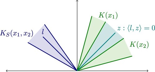
Obviously, it holds that $K_S(x^1,x^2)=\left\{0\right\}$ whenever $\mathrm{int}K\left(x^1\right)\cap \mathrm{int}K\left(x^2\right)\ne set$. In Figure 1, a cone of separations is illustrated assuming m = 2 and $K\left(x^1\right)\cap K\left(x^2\right)=\left\{0\right\}$.

Figure 1. A cone of separations for $x^1,x^2\in {\mathbb{R}}^n$ when m = 2.

The goal of this section is to relate some properties of the mapping F to those of the cone of separations. The next lemma presents some properties of $K_S(x^1,x^2)$.

Lemma 3.1

1. If $l\in K_S(x^1,x^2)$, then the hyperplane $\{z\in {\mathbb{R}}^m:〈l,z〉=0\}$ separates the cones $K\left(x^1\right)$ and $K\left(x^2\right)$.

2. $K_S(x^1,x^2)$ is a convex, closed and pointed cone.

3. If $K\left(x^1\right)\cap K\left(x^2\right)=\left\{0\right\}$, then $K_S(x^1,x^2)$ is a proper cone.

4. It is (6) $K_S(x^1,x^2)=K^{\ast }\left(x^1\right)\cap \left[-K^{\ast }\left(x^2\right)\right].$(6)

Proof.

(ii) It is easily seen that $K_S(x^1,x^2)$ is convex and closed. Suppose for a moment that $K_S(x^1,x^2)$ is not pointed, that is, there exists $l^0\in {\mathbb{R}}^m\setminus \left\{0\right\}$ with $l^0\in K_S(x^1,x^2)\cap [-K_S(x^1,x^2\left)\right].$From the previous expression, it follows that $〈l^0,z^1〉=〈l^0,z^2〉=0,$for all $z^1\in K\left(x^1\right)$ and all $z^2\in K\left(x^2\right)$. However, this is not possible since $K\left(x^1\right)$ and $K\left(x^2\right)$ are solid and, therefore, span the whole space ${\mathbb{R}}^m$.

(iii) By (ii), we only have to show that $K_S(x^1,x^2)$ is solid. By Lemma 2.1(iii) and since $K\left(x^1\right)$ and $K\left(x^2\right)$ are pointed, there exist $l^1,l^2\in {\mathbb{R}}^m$ such that $\begin{array}{rl}〈l^1,z^1& 〉\ge 0>〈l^1,z^2〉,\\ 〈l^2,z^1& 〉>0\ge 〈l^2,z^2〉,\end{array}$for all $z^1\in K\left(x^1\right)\cap S(0,1)$ and all $z^2\in K\left(x^2\right)\cap S(0,1)$. Hence, $l^1+l^2\in \text{int }{K}_S(x^1,x^2).$The statements (i) and (iv) are obvious.

The first theorem in this section relates $K_S(x^1,x^2)$ to the Jacobian of F.

Theorem 3.1

If $l\in K_S(x^1,x^2)$, then $l^T\left[DF\right(x^1)-DF(x^2\left)\right]=0$.

Proof.

Let $l\in K_S(x^1,x^2)$ and suppose that $l^T\left[DF\right(x^1)-DF(x^2\left)\right]\ne 0$. By definition, we have (7) $〈l,z^1〉\ge 0\ge 〈l,z^2〉,$(7) for all $z^1\in K\left(x^1\right)$ and $z^2\in K\left(x^2\right)$. Hence, by the K-convexity of F, (5(5) $F\left(x^1\right)-F\left(x^2\right)-DF\left(x^2\right)(x^1-x^2)\in K\left(x^2\right).$(5) ) and (7(7) $〈l,z^1〉\ge 0\ge 〈l,z^2〉,$(7) ), we get for all $x\in {\mathbb{R}}^n$ that $〈l,F\left(x\right)-F\left(x^1\right)-DF\left(x^1\right)(x-x^1)〉\ge 〈l,F\left(x\right)-F\left(x^2\right)-DF\left(x^2\right)(x-x^2)〉,$and, therefore, $〈l,F\left(x^2\right)-F\left(x^1\right)+DF\left(x^1\right)x^1-DF\left(x^2\right)x^2〉\ge 〈l,\left[DF\right(x^1)-DF(x^2\left)\right]x〉.$Now, let a real number $\alpha >0$ be arbitrarily chosen. Substituting $x=\alpha \left[DF\right(x^1)-DF(x^2){]}^{T}l$, we get $〈l,F\left(x^2\right)-F\left(x^1\right)+DF\left(x^1\right)x^1-DF\left(x^2\right)x^2〉\ge \alpha {∥l^T\left[DF\right(x^1)-DF(x^2\left)\right]∥}^2.$By $l^T\left[DF\right(x^1)-DF(x^2\left)\right]\ne 0$, letting $\alpha \to +\mathrm{\infty }$ yields a contradiction since the left-hand side of the latter inequality is finite, while its right-hand-side becomes unbounded. This completes the proof.

As a consequence, we obtain the following corollary.

Corollary 3.1

1. For all $l\in K_S(x^1,x^2)$ and all $x\in {\mathbb{R}}^n,$ we obtain $〈l,F(x+x^1)-F(x+x^2)〉\ge 〈l,F\left(x^1\right)-F\left(x^2\right)〉.$

2. If $K_S(x^1,x^2)$ is a solid cone, then $DF\left(x^1\right)=DF\left(x^2\right)$.

Proof.

(i) By (5(5) $F\left(x^1\right)-F\left(x^2\right)-DF\left(x^2\right)(x^1-x^2)\in K\left(x^2\right).$(5) ), the K-convexity of F implies $\begin{array}{rl}F(x+x^1)-F\left(x^1\right)-DF\left(x^1\right)x& \in K\left(x^1\right),\\ F(x+x^2)-F\left(x^2\right)-DF\left(x^2\right)x& \in K\left(x^2\right),\end{array}$for all $x\in {\mathbb{R}}^n$. Combining this with (7(7) $〈l,z^1〉\ge 0\ge 〈l,z^2〉,$(7) ) it follows that $〈l,F(x+x^1)-F\left(x^1\right)-DF\left(x^1\right)x〉\ge 〈l,F(x+x^2)-F\left(x^2\right)-DF\left(x^2\right)x〉,$and therefore, (8) $〈l,F(x+x^1)-F(x+x^2)〉\ge 〈l,F\left(x^1\right)-F\left(x^2\right)〉+〈l,\left[DF\right(x^1)-DF(x^2\left)\right]x〉.$(8) By Theorem 3.1, we obtain the desired result.

(ii) Since $K_S(x^1,x^2)$ is a solid cone, there exist $z\in {\mathbb{R}}^m$ and a real number $\delta >0$ such that $B(z,\delta )\subset K_S(x^1,x^2).$Then, there exist linearly independent vectors $v^i\in K_S(x^1,x^2),i=1,..,m,$ and by Theorem 3.1, we have $(v^i{)}^T\left[DF\left(x^1\right)-DF\left(x^2\right)\right]=0,i=1,..,m.$The linear independence of $v^i,i=1,..,m$ implies $DF\left(x^1\right)=DF\left(x^2\right)$.

We conclude this section by presenting its main result.

Theorem 3.2

Let $D\subset {\mathbb{R}}^n$ be an open and connected set. If there exists $\overline{y}\in {\mathbb{R}}^n$ such that $K\left(x\right)\cap K\left(\overline{y}\right)=\left\{0\right\}$ for all $x\in D$, then $F{|}_D$ is an affine mapping.

Proof.

By Lemma 3.1(iii), $K_S(x,\overline{y})$ is a solid cone for all $x\in D,$ and by Corollary 3.1(ii), we get the system $DF\left(x\right)=DF\left(\overline{y}\right),x\in D,$whose solution is $F\left(x\right)=DF\left(\overline{y}\right)(x-x^0)+F\left(x^0\right),x\in D,$for some $x^0\in D$.

Note that the fact that F has to be an affine mapping, under the assumptions of Theorem 3.2, is a surprising result given the flexibility of variable order structures.

4. Minimal variable K-convexification

In this section, we study a particular cone-valued mapping which provides a theoretical approach to obtain K-convex mappings. For a more practical approach, we refer to [16], where Bishop-Phelps and simplicial cones are used. Throughout this section assume the following:

• $C\subset {\mathbb{R}}^n$ is a convex set with $\mathrm{int}C\ne set$.

• $F:{\mathbb{R}}^n\to {\mathbb{R}}^m$ is a continuously differentiable mapping on an open neighbourhood of C.

Definition 4.1

• The set ${\mathbf{K}}_{\mathrm{conv}}\left(F\right)$ is defined as the family of all cone-valued mappings $K:C\rightrightarrows {\mathbb{R}}^m$ with the following properties:

  1. $K\left(y\right)$ is closed and convex for all $y\in C$.

  2. $F\left(x\right)-F\left(y\right)-DF\left(y\right)(x-y)\in K\left(y\right)$ for all $x,y\in C$.

• The mapping $K_F:C\rightrightarrows {\mathbb{R}}^m$ is defined by (9) $K_F\left(y\right)=\bigcap _{K\in {\mathbf{K}}_{\mathrm{c}\mathrm{o}\mathrm{n}\mathrm{v}}\left(F\right)}K\left(y\right),y\in C,$(9) and it is called the minimal variable K-convexification of F on C.

It is easily seen that $K_F\left(y\right)$ is a convex and closed cone for all $y\in C$, and that, by Lemma 2.2(i), F is $K_F$-convex on C. Note that $K_F\left(y\right)$ need not to be pointed. According to the previous definition, the minimality of $K_F\left(y\right)$ is defined with respect to all $K\in {\mathbf{K}}_{\mathrm{conv}}\left(F\right)$.

Lemma 2.2(i) implies that F is K-convex on C for all $K\in {\mathbf{K}}_{\mathrm{conv}}\left(F\right)$. Moreover, Lemma 2.2(ii) yields that $K\in {\mathbf{K}}_{\mathrm{conv}}\left(F\right)$ whenever the assumptions of Lemma 2.2 are fulfilled, that is, whenever F is K-convex on C, $\mathrm{gr}K$ is closed and $K\left(y\right)$ is convex for every $y\in C$.

The next lemma presents a specific form for the minimal variable K-convexification of F on C. For this define the mapping $\hat{F}:C\times C\to {\mathbb{R}}^m$ by $\hat{F}(x,y)=F\left(x\right)-F\left(y\right)-DF\left(y\right)(x-y),$and let $\hat{F}(C,y)=\left\{\hat{F}\right(x,y):x\in C\}$.

Lemma 4.1

For all $y\in C,$ we have $K_F\left(y\right)=\mathrm{cl}[\mathrm{coneco}\hat{F}(C,y\left)\right]$.

Proof.

By (ii) in Definition 4.1, we have for all $K\in {\mathbf{K}}_{\mathrm{conv}}\left(F\right)$ and all $x,y\in C$ that $\hat{F}(x,y)\in K\left(y\right),$and therefore, $\hat{F}(C,y)\subset K_F\left(y\right)$ for all $y\in C$. Since $K_F\left(y\right)$ is a convex and closed cone, we get $\mathrm{cl}[\mathrm{coneco}\hat{F}(C,y\left)\right]\subset K_F\left(y\right)$ for all $y\in C$.

On the other hand, $\mathrm{cl}[\mathrm{coneco}\hat{F}(C,y\left)\right]$ is a closed and convex cone for all $y\in C$ and $\hat{F}(x,y)\in \mathrm{cl}[\mathrm{coneco}\hat{F}(C,y\left)\right],$for all $x,y\in C$. Therefore, $K_F\left(y\right)\subset \mathrm{cl}[\mathrm{coneco}\hat{F}(C,y\left)\right]$ for all $y\in C$ which completes the proof.

Following [1], one is furthermore interested in conditions which are related to the existence of a proper cone $\mathcal{K}\subset {\mathbb{R}}^m$ such that (10) $K_F\left(y\right)\subset \mathcal{K},$(10) for all $y\in C$. The following lemma presents a necessary condition for this property.

Lemma 4.2

Assume that there exists a proper cone $\mathcal{K}\subset {\mathbb{R}}^m$ such that (10(10) $K_F\left(y\right)\subset \mathcal{K},$(10) ) holds for all $y\in C$. Then, there exists $w\in S(0,1)\subset {\mathbb{R}}^m$ such that the function $f_w:C\to \mathbb{R}$ given as $f_w\left(x\right)=〈w,F\left(x\right)〉$is convex on C.

Proof.

Since $K_F\left(y\right)\subset \mathcal{K}$ for all $y\in C$, by (ii) in Definition 4.1, we have (11) $\hat{F}(x,y)\in \mathcal{K},$(11) for all $x,y\in C$. Applying Lemma 2.1(i), there exist $w\in S(0,1)$ and $\delta >0$ such that (12) $〈w,z〉\ge \delta \parallel z\parallel ,$(12) for all $z\in \mathcal{K}$. By (11(11) $\hat{F}(x,y)\in \mathcal{K},$(11) ) and (12(12) $〈w,z〉\ge \delta \parallel z\parallel ,$(12) ), we get $〈w,\hat{F}(x,y)〉\ge \delta \parallel \hat{F}(x,y)\parallel \ge 0,$for all $x,y\in C$. Obviously, the latter means that $f_w$ is convex.

Our next goal is to present a sufficient condition for the existence of a proper cone $\mathcal{K}\subset {\mathbb{R}}^m$ such that (10(10) $K_F\left(y\right)\subset \mathcal{K},$(10) ) holds for all $y\in C$. For this, we assume in the remainder of this section that the set C is compact and that the mapping F is twice continuously differentiable on an open neighbourhood of C. Furthermore, for $w\in S(0,1)\subset {\mathbb{R}}^m$ define the function ${\hat{f}}_w(x,y)=〈w,\hat{F}(x,y)〉,$where $x,y\in C$.

Lemma 4.3

Assume that there exists a vector $w\in S(0,1)\subset {\mathbb{R}}^m$ such that $D^2{f}_w\left(y\right)$ is positive definite (denoted by $D^2{f}_w\left(y\right)\succ 0$) for all $y\in C$. Then, there exist real numbers $M>0,\delta >0$ such that $∥\frac{\hat{F}(x,y)}{{\hat{f}}_w(x,y)}∥<M,$for $x,y\in C$ whenever $0<\parallel x-y\parallel <\delta$.

Proof.

Suppose contrarily that there exist two sequences $\left\{x^p\right\},\left\{y^p\right\}\subset C$ such that $\underset{p}{lim}{x}^p=\underset{p}{lim}{y}^p=\overline{x},\underset{p}{lim}\frac{x^p-y^p}{∥x^p-y^p∥}=\overline{u},$and that (13) $\underset{p}{lim}∥\frac{\hat{F}(x^p,y^p)}{{\hat{f}}_w(x^p,y^p)}∥=\mathrm{\infty }.$(13) Note that $\overline{x}\in C$, since C is compact. Obviously, we have $\frac{\hat{F}(x^p,y^p)}{{\hat{f}}_w(x^p,y^p)}=\frac{\hat{F}(y^p+∥x^p-y^p∥\frac{x^p-y^p}{∥x^p-y^p∥},y^p)}{{\hat{f}}_w(y^p+∥x^p-y^p∥\frac{x^p-y^p}{∥x^p-y^p∥},y^p)}.$A componentwise ($F_i,i=1,..,m,$ denote the components of F) second-order Taylor expansion separately for each of the both parts of the latter fraction yields (14) $\underset{p}{lim}\frac{\hat{F}(x^p,y^p)}{{\hat{f}}_w(x^p,y^p)}={\left(\frac{{\overline{u}}^T{D}^2{F}_1\left(\overline{x}\right)\overline{u}}{{\overline{u}}^T{D}^2{f}_w\left(\overline{x}\right)\overline{u}},\dots ,\frac{{\overline{u}}^T{D}^2{F}_m\left(\overline{x}\right)\overline{u}}{{\overline{u}}^T{D}^2{f}_w\left(\overline{x}\right)\overline{u}}\right)}^T.$(14) By $D^2{f}_w\left(\overline{x}\right)\succ 0$, the right-hand side in (14(14) $\underset{p}{lim}\frac{\hat{F}(x^p,y^p)}{{\hat{f}}_w(x^p,y^p)}={\left(\frac{{\overline{u}}^T{D}^2{F}_1\left(\overline{x}\right)\overline{u}}{{\overline{u}}^T{D}^2{f}_w\left(\overline{x}\right)\overline{u}},\dots ,\frac{{\overline{u}}^T{D}^2{F}_m\left(\overline{x}\right)\overline{u}}{{\overline{u}}^T{D}^2{f}_w\left(\overline{x}\right)\overline{u}}\right)}^T.$(14) ) is finite which contradicts (13(13) $\underset{p}{lim}∥\frac{\hat{F}(x^p,y^p)}{{\hat{f}}_w(x^p,y^p)}∥=\mathrm{\infty }.$(13) ).

The next theorem presents a sufficient condition for the existence of a proper cone $\mathcal{K}\subset {\mathbb{R}}^m$ such that (10(10) $K_F\left(y\right)\subset \mathcal{K},$(10) ) holds for all $y\in C$. The cone $\mathcal{K}$, as defined in (16(16) $\mathcal{K}=\left\{z\in {\mathbb{R}}^m:〈Mw,z〉\ge \parallel z\parallel \right\}.$(16) ), will be later used in Lemma 4.5 as well as in Proposition 4.2.

Theorem 4.1

Assume that there exists a vector $w\in S(0,1)\subset {\mathbb{R}}^m$ such that $D^2{f}_w\left(y\right)\succ 0$ for all $y\in C$. Then, there exists a proper cone $\mathcal{K}\subset {\mathbb{R}}^m$ such that $K_F\left(y\right)\subset \mathcal{K},$for all $y\in C$.

Proof.

By Lemma 4.3, there exist real numbers $M_1>0$ and $\delta >0$ such that $∥\frac{\hat{F}(x,y)}{{\hat{f}}_w(x,y)}∥<M_1,$for $x,y\in C$ whenever $0<\parallel x-y\parallel <\delta$. Furthermore, since $D^2{f}_w\left(y\right)\succ 0$ for all $y\in C$, it follows that ${\hat{f}}_w(x,y)>0$ for all $x,y\in C$ with $x\ne y$. Hence, the fraction ${\displaystyle \frac{\hat{F}(x,y)}{{\hat{f}}_w(x,y)}}$ is defined for all $x,y\in C$ with $x\ne y$, and the compactness of C implies that there exists a real number M>1 such that (15) $∥\frac{\hat{F}(x,y)}{{\hat{f}}_w(x,y)}∥<M,$(15) for all $x,y\in C$ with $x\ne y$. Now, define the set (16) $\mathcal{K}=\left\{z\in {\mathbb{R}}^m:〈Mw,z〉\ge \parallel z\parallel \right\}.$(16) Since M>1, it is easily seen that $w\in \mathrm{int}\mathcal{K}$ and, therefore, $\mathcal{K}$ is solid. Moreover, $\mathcal{K}$ is obviously a proper cone. By (15(15) $∥\frac{\hat{F}(x,y)}{{\hat{f}}_w(x,y)}∥<M,$(15) ), we have $∥\hat{F}(x,y)∥<M{\hat{f}}_w(x,y)=M〈w,\hat{F}(x,y)〉,$for all $x,y\in C$ with $x\ne y$ and, therefore, $\hat{F}(C,y)\subset \mathcal{K}$ for all $y\in C$. Finally, by Lemma 4.1, we get $K_F\left(y\right)=\mathrm{cl}[\mathrm{coneco}\hat{F}(C,y\left)\right]\subset \mathrm{cl}\left[\mathrm{coneco}\mathcal{K}\right]=\mathcal{K},$for all $y\in C$ which completes the proof.

Note that if m = 2 and the assumptions of Theorem 4.1 hold, then we can obtain a formula for $K_F$ as follows. Let $w^0\in S(0,1)$ with $〈w,w^0〉=0$, where w is given as in Theorem 4.1. Moreover, for $y\in C,$ let (17) $\begin{array}{rl}{v}^1\left(y\right)& =\arg ma{x}_{v\in \hat{F}(C,y)\cap S(0,1)}〈v,w^0〉,\end{array}$(17) (18) $\begin{array}{rl}{v}^2\left(y\right)& =\arg mi{n}_{v\in \hat{F}(C,y)\cap S(0,1)}〈v,w^0〉.\end{array}$(18) Then, we have (19) $K_F\left(y\right)=\mathrm{coneco}\left\{v^1\right(y),v^2(y\left)\right\}.$(19) Obviously, finding $v^1\left(y\right)$ and $v^2\left(y\right)$ is not trivial and a global optimization method must be used (see, e.g. [17, Subsection 1.1.4]).

Example 4.1

Let n = m = 2, $C=[0,1{]}^2$ and $F(x_1,x_2)=\left(\begin{array}{c}{x}_1^2+x_2^2\\ x_1^3-x_2^3\end{array}\right).$Take $w=(1,0{)}^T$ and fix $w^0=(0,-1{)}^T$. By using (17(17) $\begin{array}{rl}{v}^1\left(y\right)& =\arg ma{x}_{v\in \hat{F}(C,y)\cap S(0,1)}〈v,w^0〉,\end{array}$(17) ) and (18(18) $\begin{array}{rl}{v}^2\left(y\right)& =\arg mi{n}_{v\in \hat{F}(C,y)\cap S(0,1)}〈v,w^0〉.\end{array}$(18) ), we compute $v^1\left(y\right)$, $v^2\left(y\right)$ for $y\in \left\{\right(0,0{)}^T,(0.5,0{)}^T,(1,1{)}^T\}$ and list the corresponding results in the following table:

Table

$y_1$	$y_2$	$v_1^1\left(y\right)$	$v_2^1\left(y\right)$	$v_1^2\left(y\right)$	$v_2^2\left(y\right)$
0	0	$0.71$	$-0.71$	$0.71$	$0.71$
$0.5$	0	$0.71$	$-0.71$	$0.44$	$0.89$
1	1	$0.32$	$-0.95$	$0.32$	$0.95$

This table and (19(19) $K_F\left(y\right)=\mathrm{coneco}\left\{v^1\right(y),v^2(y\left)\right\}.$(19) ) allow us to illustrate $K_F\left(y\right)$ for $y\in \left\{\right(0,0{)}^T,(0.5,0{)}^T,(1,1{)}^T\}$ in Figure 2.

Next, we deal with the Lipschitz continuity of two generators of $K_F\left(y\right)$. For this we recall the assumptions given just before Lemma 4.3, namely, that C is a compact set and F is twice continuously differentiable. We start with the following lemma.

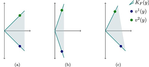
Figure 2. A minimal variable K-convexification for m = 2. (a) $y=(0,0{)}^T$, (b) $y=(0.5,0{)}^T$ and (c) $y=(1,1{)}^T$.

Lemma 4.4

1. Let $A,B\subset {\mathbb{R}}^m$ be nonempty compact sets. Then, there exist $\overline{a}\in A$ and $\overline{b}\in B$ such that ${\mathrm{\Delta }}_H(A,B)=\parallel \overline{a}-\overline{b}\parallel$ as well as ${\mathrm{\Delta }}_H(A,B)\le \parallel \overline{a}-b\parallel$ for all $b\in B$.

2. There exists $\mu >0$ such that $∥\hat{F}(x,y^1)-\hat{F}(x,y^2)∥\le \mu \parallel y^1-y^2\parallel ,$for all $x,y^1,y^2\in C$.

3. Let $a,b\in {\mathbb{R}}^m\setminus \left\{0\right\}$. Then, it holds that $∥\frac{a}{∥a∥}-\frac{b}{∥b∥}∥\le \frac{∥a-b∥}{\sqrt{∥a∥∥b∥}},$and the equality holds if and only if $\parallel a\parallel =\parallel b\parallel$.

Proof.

The compactness of A and B implies (i). Since $\hat{F}$ is continuously differentiable and C is compact, it holds that $\hat{F}$ is Lipschitz continuous on $C\times C$. Hence, there exists $\mu >0$ such that $∥\hat{F}(x,y^1)-\hat{F}(x,y^2)∥\le \mu \parallel (x,y^1)-(x,y^2)\parallel =\mu \parallel y^1-y^2\parallel ,$for all $x,y^1,y^2\in C$. For proving (iii) consider $\begin{array}{rl}{∥\frac{a}{∥a∥}-\frac{b}{∥b∥}∥}^2& =2+\frac{{∥a-b∥}^2-{∥a∥}^2-{∥b∥}^2}{∥a∥∥b∥}\\ & =\frac{{∥a-b∥}^2-{\left(∥a∥-∥b∥\right)}^2}{∥a∥∥b∥}\le \frac{{∥a-b∥}^2}{∥a∥∥b∥}.\text{■}\end{array}$

Now, we prove the Lipschitz continuity of the two generators.

Proposition 4.1

Let the set-valued mapping $G:C\rightrightarrows {\mathbb{R}}^m$ be given as $G\left(y\right)=\mathrm{c}\mathrm{o}\mathrm{n}\mathrm{v}\hat{F}(C,y).$Then, G is Lipschitz continuous on C.

Proof.

Obviously, we only have to show that there exists $\mu >0$ such that ${\mathrm{\Delta }}_H\left(G\right(y^1),G(y^2\left)\right)\le \mu \parallel y^1-y^2\parallel ,$for all $y^1,y^2\in C$. Since $G\left(y\right)$ is a compact set for all $y\in C$, by Lemma 4.4 (i), it follows that there exists ${\overline{z}}^1\in G\left(y^1\right)$ such that (20) ${\mathrm{\Delta }}_H\left(G\right(y^1),G(y^2\left)\right)\le \parallel {\overline{z}}^1-z^2\parallel ,$(20) for all $z^2\in G\left(y^2\right)$. Moreover, there exist $x^i\in C$, ${\lambda }_i\ge 0$, $i=1,\dots ,p,$ with (21) ${\overline{z}}^1=\sum _{i=1}^p{\lambda }_i\hat{F}(x^i,y^1),\sum _{i=1}^p{\lambda }_i=1.$(21) Choosing (22) $z^2=\sum _{i=1}^p{\lambda }_i\hat{F}(x^i,y^2)$(22) and substituting (21(21) ${\overline{z}}^1=\sum _{i=1}^p{\lambda }_i\hat{F}(x^i,y^1),\sum _{i=1}^p{\lambda }_i=1.$(21) ) and (22(22) $z^2=\sum _{i=1}^p{\lambda }_i\hat{F}(x^i,y^2)$(22) ) into (20(20) ${\mathrm{\Delta }}_H\left(G\right(y^1),G(y^2\left)\right)\le \parallel {\overline{z}}^1-z^2\parallel ,$(20) ), we get (23) ${\mathrm{\Delta }}_H\left(G\right(y^1),G(y^2\left)\right)\le ∥\sum _{i=1}^p{\lambda }_i\left[\hat{F}(x^i,y^1)-\hat{F}(x^i,y^2)\right]∥.$(23) Then, the statement follows by applying the triangle inequality and Lemma 4.4 (ii).

The generator used in the next result is in general not Lipschitz continuous on C. However, we present a sufficient condition for its Lipschitz continuity on a subset of C.

Lemma 4.5

Let $w\in S(0,1)\subset {\mathbb{R}}^m$, M>1 and the cone $\mathcal{K}$ be given as in (16(16) $\mathcal{K}=\left\{z\in {\mathbb{R}}^m:〈Mw,z〉\ge \parallel z\parallel \right\}.$(16) ). Assume that $v^i\in \mathcal{K}$, ${\lambda }_i\ge 0$, $i=1,\dots ,p$ and $\sum _{i=1}^p{\lambda }_i=1.$Then, we have $∥\sum _{i=1}^p{\lambda }_i{v}^i∥\ge \frac{\underset{i}{min}\parallel v^i\parallel }{M}.$

Proof.

Let Φ be an orthogonal matrix whose first row is w. Then, $∥\sum _{i=1}^p{\lambda }_i{v}^i∥=∥\mathrm{\Phi }\sum _{i=1}^p{\lambda }_i{v}^i∥\ge \sum _{i=1}^p{\lambda }_i〈w,v^i〉\ge \sum _{i=1}^p{\lambda }_i\frac{\parallel v^i\parallel }{M}\ge \frac{\underset{i}{min}\parallel v^i\parallel }{M}.\text{■}$

As mentioned just before Lemma 4.5, the next result yields a sufficient condition for a generator to be Lipschitz continuous (only) on a subset $A\subset C$. Here, we have to ‘cut out’ a subset from $\hat{F}(C,y)$. We refer also to Remark 4.1, where we discuss how, under certain conditions, this result could be used.

Proposition 4.2

Let $A\subset C$ be a compact convex set. Assume that for some $w\in S(0,1)\subset {\mathbb{R}}^m$ it holds that $D^2{f}_w\left(y\right)\succ 0$ for all $y\in C$, and that there exists $\delta >0$ such that (24) $K_F\left(y\right)=\mathrm{coneco}\left[\hat{F}(C,y)\setminus \mathrm{i}\mathrm{n}\mathrm{t}B(0,\delta )\right],$(24) for all $y\in A$. Then, the set-valued mapping $G:A\rightrightarrows {\mathbb{R}}^m$, given as $G\left(y\right)=K_F\left(y\right)\cap S(0,1),$is Lipschitz continuous on A.

Proof.

We will prove that G is locally Lipschitz continuous for any arbitrarily chosen $\overline{y}\in A$. Then, the Lipschitz continuity of G on A follows from the convexity and the compactness of A. By Theorem 4.1, there exists a proper cone $\mathcal{K}$ such that $K_F\left(y\right)\subset \mathcal{K},$where $\mathcal{K}$ is given as in (16(16) $\mathcal{K}=\left\{z\in {\mathbb{R}}^m:〈Mw,z〉\ge \parallel z\parallel \right\}.$(16) ) for certain M>1. Let $\mu >0$ be given as in Lemma 4.4 (ii). Choose $y^1,y^2\in B\left(\overline{y},\frac{\delta }{4\mu }\right)\cap A.$By Lemma 4.4 (ii), we have (25) $\parallel \hat{F}(x,y^2)\parallel \ge \frac{\delta }{2},$(25) whenever $\parallel \hat{F}(x,y^1)\parallel \ge \delta$ for $x\in C$. Next, we will show that (26) ${\mathrm{\Delta }}_H\left(G\right(y^1),G(y^2\left)\right)\le \frac{\sqrt{2}\mu M}{\delta }\parallel y^1-y^2\parallel .$(26) Analogously to the proof of Proposition 4.1, by (24(24) $K_F\left(y\right)=\mathrm{coneco}\left[\hat{F}(C,y)\setminus \mathrm{i}\mathrm{n}\mathrm{t}B(0,\delta )\right],$(24) ), we get (27) ${\mathrm{\Delta }}_H\left(G\right(y^1),G(y^2\left)\right)\le ∥\frac{\sum _{i=1}^p{\lambda }_i\hat{F}(x^i,y^1)}{∥\sum _{i=1}^p{\lambda }_i\hat{F}(x^i,y^1)∥}-\frac{\sum _{i=1}^p{\lambda }_i\hat{F}(x^i,y^2)}{∥\sum _{i=1}^p{\lambda }_i\hat{F}(x^i,y^2)∥}∥$(27) with (28) $\parallel \hat{F}(x^i,y^1)\parallel \ge \delta ,\parallel \hat{F}(x^i,y^2)\parallel \ge \frac{\delta }{2},i=1,\dots ,p,\sum _{i=1}^p{\lambda }_i=1.$(28) Note that in (28(28) $\parallel \hat{F}(x^i,y^1)\parallel \ge \delta ,\parallel \hat{F}(x^i,y^2)\parallel \ge \frac{\delta }{2},i=1,\dots ,p,\sum _{i=1}^p{\lambda }_i=1.$(28) ), the two inequalities follow from (24(24) $K_F\left(y\right)=\mathrm{coneco}\left[\hat{F}(C,y)\setminus \mathrm{i}\mathrm{n}\mathrm{t}B(0,\delta )\right],$(24) ) and (25(25) $\parallel \hat{F}(x,y^2)\parallel \ge \frac{\delta }{2},$(25) ), respectively. By Lemma 4.4 (iii) and (27(27) ${\mathrm{\Delta }}_H\left(G\right(y^1),G(y^2\left)\right)\le ∥\frac{\sum _{i=1}^p{\lambda }_i\hat{F}(x^i,y^1)}{∥\sum _{i=1}^p{\lambda }_i\hat{F}(x^i,y^1)∥}-\frac{\sum _{i=1}^p{\lambda }_i\hat{F}(x^i,y^2)}{∥\sum _{i=1}^p{\lambda }_i\hat{F}(x^i,y^2)∥}∥$(27) ), we get (29) ${\mathrm{\Delta }}_H\left(G\right(y^1),G(y^2\left)\right)\le \frac{∥\sum _{i=1}^p{\lambda }_i\left[\hat{F}(x^i,y^1)-\hat{F}(x^i,y^2)\right]∥}{\sqrt{∥\sum _{i=1}^p{\lambda }_i\hat{F}(x^i,y^1)∥∥\sum _{i=1}^p{\lambda }_i\hat{F}(x^i,y^2)∥}}.$(29) Moreover, by Lemma 4.5 and (28(28) $\parallel \hat{F}(x^i,y^1)\parallel \ge \delta ,\parallel \hat{F}(x^i,y^2)\parallel \ge \frac{\delta }{2},i=1,\dots ,p,\sum _{i=1}^p{\lambda }_i=1.$(28) ), it follows that (30) $∥\sum _{i=1}^p{\lambda }_i\hat{F}(x^i,y^1)∥\ge \frac{\delta }{M},∥\sum _{i=1}^p{\lambda }_i\hat{F}(x^i,y^2)∥\ge \frac{\delta }{2M}.$(30) Finally, applying the triangle inequality, Lemma 4.4 (ii) and using (30(30) $∥\sum _{i=1}^p{\lambda }_i\hat{F}(x^i,y^1)∥\ge \frac{\delta }{M},∥\sum _{i=1}^p{\lambda }_i\hat{F}(x^i,y^2)∥\ge \frac{\delta }{2M}.$(30) ) in (29(29) ${\mathrm{\Delta }}_H\left(G\right(y^1),G(y^2\left)\right)\le \frac{∥\sum _{i=1}^p{\lambda }_i\left[\hat{F}(x^i,y^1)-\hat{F}(x^i,y^2)\right]∥}{\sqrt{∥\sum _{i=1}^p{\lambda }_i\hat{F}(x^i,y^1)∥∥\sum _{i=1}^p{\lambda }_i\hat{F}(x^i,y^2)∥}}.$(29) ), we obtain (26(26) ${\mathrm{\Delta }}_H\left(G\right(y^1),G(y^2\left)\right)\le \frac{\sqrt{2}\mu M}{\delta }\parallel y^1-y^2\parallel .$(26) ).

Remark 4.1

Proposition 4.2 can be exploited in the following way. Let $A\subset C$ be a set for which the assumptions of Proposition 4.2 are fulfilled. Choose a cone-valued mapping $K_A:C\rightrightarrows {\mathbb{R}}^m$ with $K_A\left(y\right)=\left\{\begin{array}{ll}{K}_F\left(y\right)& \text{if }y\in A,\\ K& \text{if }y\in C\setminus A,\end{array}\right.$where $K\subset {\mathbb{R}}^m$ is a fixed cone satisfying $K_F\left(y\right)=K$ for $y\in \mathrm{bd}A$ and $K_F\left(y\right)\subset K$ for $y\in C\setminus A$. Define the set-valued mapping $G_A\left(y\right)=K_A\left(y\right)\cap S(0,1).$Since $S(0,1)$ is bounded, the Hausdorff distance is a metric for the family of compact subsets of $S(0,1)$ (see, e.g. [15, Section 4C]). A moment of reflection shows that $G_A$ is continuous on C whenever its codomain is endowed with this metric. Moreover, by Proposition 4.2, it follows that $G_A$ is Lipschitz continuous on A and, by definition, that $G_A$ is Lipschitz continuous on $C\setminus A$. Consequently, $G_A$ is Lipschitz continuous on C. We will come back to this approach at the end of Section 5. Of course, such a choice of $K_A$ is not always possible. Necessary or sufficient conditions for its existence will be considered in future research.

5. A particular case

In this section, we study a particular case and apply to it the general approach described in the previous sections. Specifically, we consider an interval $[\alpha ,\text{β}]\subset \mathbb{R}$ and a mapping $F\in {\mathcal{C}}^2\left(\right[\alpha ,\text{β}],{\mathbb{R}}^2)$, $F\left(t\right)=\left(F_1\right(t),F_2(t\left)\right)$. Moreover, we assume that $F_1^{\mathrm{\prime }\mathrm{\prime }}\left(t\right)>0$, $t\in [\alpha ,\text{β}]$, where $F_i^{\mathrm{\prime }}\left(t\right)$ and $F_i^{\mathrm{\prime }\mathrm{\prime }}\left(t\right)$, $i=1,2,$ denote the first and second derivative at $t\in \mathbb{R}$, respectively. For this case, we obtain a particular expression for $K_F\left(t\right)$. First, we define four auxiliary functions.

Lemma 5.1

Let $t_0\in [\alpha ,\text{β}]$ and define $\begin{array}{rl}{\varphi }_{-}\left(t\right)& ={\hat{F}}_1(t,t_0),t\in [\alpha ,t_0],\\ {\varphi }_{+}\left(t\right)& ={\hat{F}}_1(t,t_0),t\in [t_0,\text{β}].\end{array}$Then, ${\varphi }_{-}$ is strictly decreasing, and ${\varphi }_{+}$ is strictly increasing.

Proof.

For ${\varphi }_{+}$ we get ${\varphi }_{+}^{\mathrm{\prime }}\left(t\right)=F_1^{\mathrm{\prime }}\left(t\right)-F_1^{\mathrm{\prime }}\left(t_0\right)=F_1^{\mathrm{\prime }\mathrm{\prime }}\left({\theta }_t\right)(t-t_0)$for some ${\theta }_t\in (t_0,\text{β})$. Since $F_1^{\mathrm{\prime }\mathrm{\prime }}\left(t\right)>0$, $t\in [t_0,\text{β}]$, it holds that ${\varphi }_{+}$ is strictly increasing. Analogously, we obtain that ${\varphi }_{-}$ is strictly decreasing.

Since ${\hat{F}}_1(t_0,t_0)=0$, Lemma 5.1 yields for $t_0\in [\alpha ,\text{β}]$ that ${\hat{F}}_1(t,t_0)>0,$for all $t\in [\alpha ,\text{β}]\setminus \left\{t_0\right\}$. Moreover, by Lemma 5.1, both ${\varphi }_{-}$ and ${\varphi }_{+}$ are injective functions. Therefore, the functions ${\psi }_{-}:[0,{\varphi }_{-}(\alpha \left)\right]\to [0,{\hat{F}}_2(\alpha ,t_0\left)\right]$ and ${\psi }_{+}:[0,{\varphi }_{+}(\text{β}\left)\right]\to [0,{\hat{F}}_2(\text{β},t_0\left)\right]$, given by $\begin{array}{rl}{\psi }_{-}\left(x\right)& ={\hat{F}}_2\left({\varphi }_{-}^{-1}\left(x\right),t_0\right),\\ {\psi }_{+}\left(x\right)& ={\hat{F}}_2\left({\varphi }_{+}^{-1}\left(x\right),t_0\right),\end{array}$are well defined. The following two results concern the relationship between the latter two functions and $\hat{F}(t,t_0)$.

Lemma 5.2

The right derivatives of ${\psi }_{-}$ and ${\psi }_{+}$ at x = 0 are ${\psi }_{-}^{\mathrm{\prime }}\left(0\right)={\psi }_{+}^{\mathrm{\prime }}\left(0\right)=\frac{F_2^{\mathrm{\prime }\mathrm{\prime }}\left(t_0\right)}{F_1^{\mathrm{\prime }\mathrm{\prime }}\left(t_0\right)}.$

Proof.

We show it for ${\psi }_{+}$. Since ${\psi }_{+}\left(0\right)=0$, we have (31) ${\psi }_{+}^{\mathrm{\prime }}\left(0\right)=\underset{\mathrm{\Delta }x\to 0^{+}}{lim}\frac{{\psi }_{+}\left(\mathrm{\Delta }x\right)}{\mathrm{\Delta }x}=\underset{t\to t_0^{+}}{lim}\frac{{\hat{F}}_2(t,t_0)}{{\hat{F}}_1(t,t_0)}.$(31) After applying L'Hôpital's rule twice we get the desired result. The proof runs analogously for ${\psi }_{-}$.

Lemma 5.3

If $\frac{F_2^{\mathrm{\prime }\mathrm{\prime }}\left(t\right)}{F_1^{\mathrm{\prime }\mathrm{\prime }}\left(t\right)}$ is an increasing function on $[\alpha ,\text{β}]$, then ${\psi }_{-}\left(x\right)$ is concave and ${\psi }_{+}\left(x\right)$ is convex.

Proof.

For showing the convexity of ${\psi }_{+}$, we prove that (32) ${\psi }_{+}^{\mathrm{\prime }\mathrm{\prime }}\left(x\right)>0,$(32) for all $x\in (0,{\varphi }_{+}(\text{β}\left)\right)$. For $x\in (0,{\varphi }_{+}(\text{β}\left)\right)$ and $t={\varphi }_{+}^{-1}\left(x\right)$, after a straightforward calculation, we get that ${\psi }_{+}^{\mathrm{\prime }\mathrm{\prime }}\left(x\right)=\frac{F_2^{\mathrm{\prime }\mathrm{\prime }}\left(t\right)-F_1^{\mathrm{\prime }\mathrm{\prime }}\left(t\right)\left[{\displaystyle \frac{F_2^{\mathrm{\prime }}\left(t\right)-F_2^{\mathrm{\prime }}\left(t_0\right)}{F_1^{\mathrm{\prime }}\left(t\right)-F_1^{\mathrm{\prime }}\left(t_0\right)}}\right]}{{\left[F_1^{\mathrm{\prime }}\left(t\right)-F_1^{\mathrm{\prime }}\left(t_0\right)\right]}^2}.$Since $F_1^{\mathrm{\prime }\mathrm{\prime }}\left(t\right)>0$, in order to obtain (32(32) ${\psi }_{+}^{\mathrm{\prime }\mathrm{\prime }}\left(x\right)>0,$(32) ), we use that $\frac{F_2^{\mathrm{\prime }\mathrm{\prime }}\left(t\right)}{F_1^{\mathrm{\prime }\mathrm{\prime }}\left(t\right)}>\frac{F_2^{\mathrm{\prime }}\left(t\right)-F_2^{\mathrm{\prime }}\left(t_0\right)}{F_1^{\mathrm{\prime }}\left(t\right)-F_1^{\mathrm{\prime }}\left(t_0\right)}.$By Cauchy's mean value theorem, the latter inequality holds since $t>t_0$, and $\frac{F_2^{\mathrm{\prime }\mathrm{\prime }}\left(t\right)}{F_1^{\mathrm{\prime }\mathrm{\prime }}\left(t\right)}$ is an increasing function on $[\alpha ,\text{β}]$. The concavity of ${\psi }_{-}$ is obtained analogously.

In the remainder of this section, we assume that $\frac{F_2^{\mathrm{\prime }\mathrm{\prime }}\left(t\right)}{F_1^{\mathrm{\prime }\mathrm{\prime }}\left(t\right)}$ is increasing on $[\alpha ,\text{β}]$. The next result is a consequence of Lemma 5.3.

Corollary 5.1

Let $t_0\in (\alpha ,\text{β})$. Then, we have $\frac{{\hat{F}}_2(\alpha ,t_0)}{{\hat{F}}_1(\alpha ,t_0)}\le \frac{{\hat{F}}_2(t,t_0)}{{\hat{F}}_1(t,t_0)}\le \frac{{\hat{F}}_2(\text{β},t_0)}{{\hat{F}}_1(\text{β},t_0)},$for all $t\in [\alpha ,\text{β}]\setminus \left\{t_0\right\}$.

Proof.

If $t>t_0$, then for $x={\varphi }_{+}\left(t\right),$ we have $x\in (0,{\varphi }_{+}(\text{β}\left)\right]$. By the convexity of ${\psi }_{+}$, Lemma 5.2 implies $\frac{F_2^{\mathrm{\prime }\mathrm{\prime }}\left(t_0\right)}{F_1^{\mathrm{\prime }\mathrm{\prime }}\left(t_0\right)}\le \frac{{\psi }_{+}\left(x\right)}{x}\le \frac{{\psi }_{+}\left({\varphi }_{+}\right(\text{β}\left)\right)}{{\varphi }_{+}\left(\text{β}\right)}.$Hence, we obtain $\frac{F_2^{\mathrm{\prime }\mathrm{\prime }}\left(t_0\right)}{F_1^{\mathrm{\prime }\mathrm{\prime }}\left(t_0\right)}\le \frac{{\hat{F}}_2(t,t_0)}{{\hat{F}}_1(t,t_0)}\le \frac{{\hat{F}}_2(\text{β},t_0)}{{\hat{F}}_1(\text{β},t_0)}$and, analogously, for $t<t_0$ that $\frac{{\hat{F}}_2(\alpha ,t_0)}{{\hat{F}}_1(\alpha ,t_0)}\le \frac{{\hat{F}}_2(t,t_0)}{{\hat{F}}_1(t,t_0)}\le \frac{F_2^{\mathrm{\prime }\mathrm{\prime }}\left(t_0\right)}{F_1^{\mathrm{\prime }\mathrm{\prime }}\left(t_0\right)}.$A combination of these two results delivers for $t>t_0$ that $\frac{{\hat{F}}_2(\alpha ,t_0)}{{\hat{F}}_1(\alpha ,t_0)}\le \frac{F_2^{\mathrm{\prime }\mathrm{\prime }}\left(t_0\right)}{F_1^{\mathrm{\prime }\mathrm{\prime }}\left(t_0\right)}\le \frac{{\hat{F}}_2(t,t_0)}{{\hat{F}}_1(t,t_0)}\le \frac{{\hat{F}}_2(\text{β},t_0)}{{\hat{F}}_1(\text{β},t_0)},$and a corresponding result for $t<t_0$. This completes the proof.

In the next result, we see the advantage of considering $F\in {\mathcal{C}}^2\left(\right[\alpha ,\text{β}],{\mathbb{R}}^2)$. We show that in this case, the minimal variable K-convexification of F on $[\alpha ,\text{β}]$ can easily and directly be calculated.

Theorem 5.1

Let the mappings $G_{\alpha }:[\alpha ,\text{β}]\to {\mathbb{R}}^2$ and $G_{\text{β}}:[\alpha ,\text{β}]\to {\mathbb{R}}^2$ be given as $G_{\alpha }\left(t_0\right)=\left\{\begin{array}{ll}{F}^{\mathrm{\prime }\mathrm{\prime }}\left(\alpha \right)& \text{if }{t}_0=\alpha ,\\ \hat{F}(\alpha ,t_0)& \text{if }\alpha <t_0\le \text{β},\end{array}\right.G_{\text{β}}\left(t_0\right)=\left\{\begin{array}{ll}\hat{F}(\text{β},t_0)& \text{if }\alpha \le t_0<\text{β},\\ F^{\mathrm{\prime }\mathrm{\prime }}\left(\text{β}\right)& \text{if }{t}_0=\text{β}\end{array}\right.$and define the set-valued mapping $G\left(t_0\right)=\left\{G_{\alpha }\right(t_0),G_{\text{β}}(t_0\left)\right\}$. Then, $K_F\left(t_0\right)=\mathrm{coneco}G\left(t_0\right)$.

Proof.

We distinguish two cases.

Case 1: Let $t_0\in (\alpha ,\text{β})$. Then, we have $G\left(t_0\right)=\left\{\hat{F}(\alpha ,t_0),\hat{F}(\text{β},t_0)\right\}\subset \hat{F}\left(\right[\alpha ,\text{β}],t_0).$Hence, it holds that (33) $\mathrm{coneco}G\left(t_0\right)\subset \mathrm{coneco}\hat{F}\left(\right[\alpha ,\text{β}],t_0).$(33) Next, we prove that (34) $\hat{F}\left(\right[\alpha ,\text{β}],t_0)\subset \mathrm{coneco}G\left(t_0\right).$(34) Note that $0\in \mathrm{coneco}G\left(t_0\right)$. Now, choose $z\in \hat{F}\left(\right[\alpha ,\text{β}],t_0)\setminus \left\{0\right\}$. Therefore, there exists $t\in [\alpha ,\text{β}]\setminus \left\{t_0\right\}$ such that $z=\hat{F}(t,t_0)$. From Corollary 5.1, it follows for $z=(z_1,z_2)$ that $z_1={\hat{F}}_1(t,t_0)>0$ and that $\frac{{\hat{F}}_2(\alpha ,t_0)}{{\hat{F}}_1(\alpha ,t_0)}\le \frac{z_2}{z_1}\le \frac{{\hat{F}}_2(\text{β},t_0)}{{\hat{F}}_1(\text{β},t_0)}.$Thus, there exists $\lambda \in [0,1]$ such that $\frac{z_2}{z_1}=\lambda \frac{{\hat{F}}_2(\alpha ,t_0)}{{\hat{F}}_1(\alpha ,t_0)}+(1-\lambda )\frac{{\hat{F}}_2(\text{β},t_0)}{{\hat{F}}_1(\text{β},t_0)}.$A moment of reflection shows that the latter equation yields (35) $z=\frac{\lambda z_1}{{\hat{F}}_1(\alpha ,t_0)}\hat{F}(\alpha ,t_0)+\frac{(1-\lambda )z_1}{{\hat{F}}_1(\text{β},t_0)}\hat{F}(\text{β},t_0).$(35) Note that in (35(35) $z=\frac{\lambda z_1}{{\hat{F}}_1(\alpha ,t_0)}\hat{F}(\alpha ,t_0)+\frac{(1-\lambda )z_1}{{\hat{F}}_1(\text{β},t_0)}\hat{F}(\text{β},t_0).$(35) ) the coefficients of $\hat{F}(\alpha ,t_0)$ and $\hat{F}(\text{β},t_0)$ are nonnegative since $\lambda \in [0,1]$, $z_1>0$, ${\hat{F}}_1(\alpha ,t_0)>0$ and ${\hat{F}}_1(\text{β},t_0)>0$. Thus, (34(34) $\hat{F}\left(\right[\alpha ,\text{β}],t_0)\subset \mathrm{coneco}G\left(t_0\right).$(34) ) is shown. By Lemma 4.1, (33(33) $\mathrm{coneco}G\left(t_0\right)\subset \mathrm{coneco}\hat{F}\left(\right[\alpha ,\text{β}],t_0).$(33) ) and (34(34) $\hat{F}\left(\right[\alpha ,\text{β}],t_0)\subset \mathrm{coneco}G\left(t_0\right).$(34) ), we get $K_F\left(t_0\right)=\mathrm{coneco}G\left(t_0\right)$.

Case 2: Let $t_0=\alpha$ (analogously for $t_0=\text{β}$). Applying L'Hôpital's rule twice, we get $\underset{t\to {\alpha }^{-}}{lim}\frac{{\hat{F}}_2(t,\alpha )}{{\hat{F}}_1(t,\alpha )}=\frac{F_2^{\mathrm{\prime }\mathrm{\prime }}\left(\alpha \right)}{F_1^{\mathrm{\prime }\mathrm{\prime }}\left(\alpha \right)},$and by $G\left(\alpha \right)=\left\{F^{\mathrm{\prime }\mathrm{\prime }}\right(\alpha ),\hat{F}(\text{β},\alpha \left)\right\}$, we get $G\left(\alpha \right)\subset \mathrm{cl}\mathrm{coneco}\hat{F}\left(\right[\alpha ,\text{β}],\alpha ).$Moreover, letting $t_0\to \alpha$ in Corollary 5.1, we obtain (36) $\frac{F_2^{\mathrm{\prime }\mathrm{\prime }}\left(\alpha \right)}{F_1^{\mathrm{\prime }\mathrm{\prime }}\left(\alpha \right)}\le \frac{{\hat{F}}_2(t,\alpha )}{{\hat{F}}_1(t,\alpha )}\le \frac{{\hat{F}}_2(\text{β},\alpha )}{{\hat{F}}_1(\text{β},\alpha )}.$(36) Using (36(36) $\frac{F_2^{\mathrm{\prime }\mathrm{\prime }}\left(\alpha \right)}{F_1^{\mathrm{\prime }\mathrm{\prime }}\left(\alpha \right)}\le \frac{{\hat{F}}_2(t,\alpha )}{{\hat{F}}_1(t,\alpha )}\le \frac{{\hat{F}}_2(\text{β},\alpha )}{{\hat{F}}_1(\text{β},\alpha )}.$(36) ) we deduce an expression which is analogous to (35(35) $z=\frac{\lambda z_1}{{\hat{F}}_1(\alpha ,t_0)}\hat{F}(\alpha ,t_0)+\frac{(1-\lambda )z_1}{{\hat{F}}_1(\text{β},t_0)}\hat{F}(\text{β},t_0).$(35) ). The remaining part of the proof runs as in Case 1.

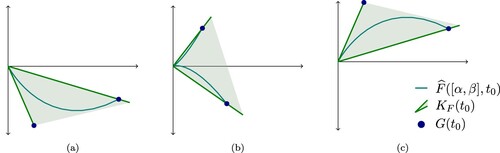
Example 5.1

Let $\alpha =-1$, $\text{β}=1$ and $F\left(t\right)=(t^2,t^3{)}^T$. By using Theorem 5.1, we have $K_F\left(t_0\right)=\mathrm{coneco}G\left(t_0\right)$ for $t_0\in \{-1,0.15,1\}$, which is illustrated in Figure 3.

Figure 3. Application of Theorem 5.1 for $F\left(t\right)=(t^2,t^3{)}^T$ with $\alpha =-1$ and $\text{β}=1$. (a) $t_0=-1$, (b) $t_0=0.15$ and (c) $t_0=1$.

Note that the set-valued mapping $G\left(t_0\right)$ in Theorem 5.1 is not Lipschitz continuous. Indeed, since $\underset{t_0\to \alpha }{lim}{G}_{\alpha }\left(t_0\right)=\underset{t_0\to \alpha }{lim}\hat{F}(\alpha ,t_0)=0\text{and}{G}_{\alpha }\left(\alpha \right)=F^{\mathrm{\prime }\mathrm{\prime }}\left(\alpha \right)\ne 0,$the function $G_{\alpha }\left(t_0\right)$ is not continuous. However, we can find a cone-valued mapping $K_{\delta }\left(t_0\right)$ close to $K_F\left(t_0\right)$ such that its generator mapping is Lipschitz continuous. As an example, fix $\delta >0$, define $\begin{array}{rl}{G}_{\alpha }^{\delta }\left(t_0\right)& =\left\{\begin{array}{ll}\hat{F}(\alpha ,\alpha +\delta )& \text{if }\alpha \le t_0\le \alpha +\delta ,\\ \hat{F}(\alpha ,t_0)& \text{if }\alpha +\delta <t_0\le \text{β},\end{array}\right.\\ G_{\text{β}}^{\delta }\left(t_0\right)& =\left\{\begin{array}{ll}\hat{F}(\text{β},t_0)& \text{if }\alpha \le t_0<\text{β}-\delta ,\\ \hat{F}(\text{β},\text{β}-\delta )& \text{if }\text{β}-\delta \le t_0\le \text{β}\end{array}\right.\end{array}$and set $K_{\delta }\left(t_0\right)=\mathrm{coneco}\left[G_{\alpha }^{\delta }\left(t_0\right),G_{\text{β}}^{\delta }\left(t_0\right)\right].$Analogously to Proposition 4.2, it can be shown that $K_{\delta }\left(t_0\right)\cap S(0,1)$ is Lipschitz continuous on $[\alpha ,\text{β}]$. Moreover, it is easy to check that $K_F\left(t_0\right)=K_{\delta }\left(t_0\right),$for all $t_0\in [\alpha +\delta ,\text{β}-\delta ]$ and that $K_F\left(t_0\right)⊊K_{\delta }\left(t_0\right),$for all $t_0\in [\alpha ,\text{β}]\setminus [\alpha +\delta ,\text{β}-\delta ]$. This latter construction represents an application of the strategy described in Remark 4.1 to this particular case considered in the current section.

6. Final remarks

In this paper, we considered vector optimization problems with variable ordering structures. They are related to K-convex mappings where K refers to a proper cone-valued mapping. This model has several applications, e.g. in medical diagnosis and portfolio optimization. We defined the cone of separations and showed that under certain assumptions the corresponding K-convex mapping needs to be affine. Note that this is a somehow counter-intuitive property and its geometric meaning need still to be discussed in the future. Moreover, we introduced the concept of the minimal variable K-convexification $K_F\left(x\right)$, presented sufficient conditions for the images of this cone-valued mapping to be contained in a proper cone and proved the Lipschitz continuity of some corresponding generator mappings. Note that we described a theoretical approach for generating a variable ordering mapping for which a given mapping is K-convex. We applied this approach to a particular case; the construction of further applications will be a topic for further research.

Disclosure statement

No potential conflict of interest was reported by the author(s).

References

- Bello Cruz JY, Bouza Allende G. A steepest descent-like method for variable order vector optimization problems. J Optim Theory Appl. 2014;162:371–391.
- Graña Drummond LM, Iusem AN. A projected gradient method for vector optimization problems. Comput Optim Appl. 2004;28(1):5–29.
- Graña Drummond LM, Svaiter BF. A steepest descent method for vector optimization. J Comput Appl Math. 2005;175(2):395–414.
- Luc DT. Theory of vector optimization. New York (NY): Springer; 1989.
- Luc DT, Tan NX, Tinh PN. Convex vector functions and their subdifferential. Acta Math. 1998;23(1):107–127.
- Bello Cruz JY, Bouza Allende G. On inexact projected gradient methods for solving variable vector optimization problems. Optim Eng. 2020. Available from: https://doi.org/10.1007/s11081-020-09579-8
- Durea M, Strugariu R, Tammer C. On set-valued optimization problems with variable ordering structure. J Global Optim. 2015;61:745–767.
- Engau A. Variable preference modeling with ideal-symmetric convex cones. J Global Optim. 2008;42:295–311.
- Wacker M, Deinzer F. Automatic robust medical image registration using a new democratic vector optimization approach with multiple measures. In: Yang GZ, editor. Medical image computing and computer-assisted intervention – MICCAI. New York: Springer; 2009.
- Eichfelder G. Variable ordering structures in vector optimization. New York (NY): Springer; 2014.
- Boyd S, Vandenberghe L. Convex optimization. Cambridge: Cambridge University Press; 2009.
- Dattorro J. Convex optimization & Euclidean distance geometry. Palo Alto (CA): Meboo Publishing USA; 2013.
- Jahn J. Vector optimization: theory, applications and extensions. New York (NY): Springer; 2011.
- Mordukhovich BS. Variational analysis and generalized differentiation. New York (NY): Springer; 2006.
- Rockafellar RT, Wets RJ. Variational analysis. New York (NY): Springer; 1998.
- Bouza Allende G, Hernández Escobar D, Rückmann J-J. Generation of K-convex test problems in variable ordering settings. Rev Inv Oper. 2018;39(3):463–479.
- Pintér JD. Global optimization in action. New York (NY): Springer; 1996.