Lipschitz upper semicontinuity in linear optimization via local directional convexity

Abstract

This work is focussed on computing the Lipschitz upper semicontinuity modulus of the argmin mapping for canonically perturbed linear programs. The immediate antecedent can be traced out from Camacho J et al. [2022. From calmness to Hoffman constants for linear semi-infinite inequality systems. Available from: https://arxiv.org/pdf/2107.10000v2.pdf], devoted to the feasible set mapping. The aimed modulus is expressed in terms of a finite amount of calmness moduli, previously studied in the literature. Despite the parallelism in the results, the methodology followed in the current paper differs notably from Camacho J et al. [2022] as far as the graph of the argmin mapping is not convex; specifically, a new technique based on a certain type of local directional convexity is developed.

Keywords:

• Lipschitz upper semicontinuity
• calmness
• argmin mapping
• linear programming

Mathematics Subject Classifications:

• 90C31
• 49J53
• 49K40
• 15A39
• 90C05

1. Introduction and motivation

The main goal of the present paper is to compute the upper semicontinuity modulus of the optimal set (argmin) mapping associated with the parameterized linear programming (LP, in brief) problem given by (1) $\begin{array}{rll}\pi :& \mathrm{m}\mathrm{i}\mathrm{n}\mathrm{i}\mathrm{m}\mathrm{i}\mathrm{z}\mathrm{e}& c^{\mathrm{\prime }}x\\ & \mathrm{s}\mathrm{u}\mathrm{b}\mathrm{j}\mathrm{e}\mathrm{c}\mathrm{t}\mathrm{t}\mathrm{o}& a_t^{\mathrm{\prime }}x\le b_t,t\in T:=\{1,2,\dots ,m\},\end{array}$(1) where $x\in {\mathbb{R}}^n$ is the decision variable, regarded as a column-vector, the prime stands for transposition, $a_t\in {\mathbb{R}}^n$ is fixed for each $t\in T$, and the pair $(c,b)\in {\mathbb{R}}^n\times {\mathbb{R}}^m$, with $b=(b_t{)}_{t\in T}\in {\mathbb{R}}^m$, is the parameter to be perturbed around a nominal one $(\overline{c},\overline{b})\in {\mathbb{R}}^n\times {\mathbb{R}}^m$. In this way we are dealing with the so-called canonical perturbations (tilt perturbations of the objective function together with the right-hand side – RHS – of the constraints). We consider the feasible set and the optimal set mappings $\mathcal{F}:{\mathbb{R}}^m\rightrightarrows {\mathbb{R}}^n$ and ${\mathcal{F}}^{op}:{\mathbb{R}}^n\times {\mathbb{R}}^m\rightrightarrows {\mathbb{R}}^n$ defined as (2) $\begin{array}{rl}\mathcal{F}\left(b\right)& :=\{x\in {\mathbb{R}}^n:a_t^{\mathrm{\prime }}x\le b_t\mathrm{f}\mathrm{o}\mathrm{r}\mathrm{a}\mathrm{l}\mathrm{l}t\in T\},\end{array}$(2) (3) $\begin{array}{rl}{\mathcal{F}}^{op}\left(\pi \right)& :=\arg min\{c^{\mathrm{\prime }}x:x\in \mathcal{F}\left(b\right)\}.\end{array}$(3) From now on we identify each problem π with the corresponding parameter $(c,b);$ accordingly, $\overline{\pi }\equiv (\overline{c},\overline{b})$ denotes the nominal problem. The space of variables, ${\mathbb{R}}^n$, is endowed with an arbitrary norm $\Vert \cdot \Vert$, whose dual norm is denoted by $\Vert \cdot {\Vert }_{\ast }$, i.e. $\Vert u{\Vert }_{\ast }=\underset{\Vert x\Vert \le 1}{max}|u^{\mathrm{\prime }}x|$. The parameter space ${\mathbb{R}}^n\times {\mathbb{R}}^m$ is endowed with the norm $\Vert (c,b)\Vert :=max\{\Vert c{\Vert }_{\ast },\Vert b{\Vert }_{\mathrm{\infty }}\}$(since c is identified with the linear functional $x\mapsto c^{\mathrm{\prime }}x)$, where $\Vert b{\Vert }_{\mathrm{\infty }}:=\underset{t\in T}{max}\left|b_t\right|$.

The current paper is mainly oriented to the computation of the Lipschitz upper semicontinuity modulus of ${\mathcal{F}}^{op}$ at the nominal parameter $\overline{\pi }$, denoted by $\mathrm{Lipusc}{\mathcal{F}}^{op}\left(\overline{\pi }\right)$ following [1]; see Section 2 for the formal definitions. At this moment let us comment that $\mathrm{Lipusc}{\mathcal{F}}^{op}\left(\overline{\pi }\right)$ provides a semi-local measure of the stability (in fact, a rate of deviation) of the optimal set around the nominal problem $\overline{\pi }$. The term ‘semi-local’ refers to the fact that only parameters π around $\overline{\pi }$ are considered, while all elements of ${\mathcal{F}}^{op}\left(\pi \right)$ are taken into account. A point-based formula (only depending on the nominal data $(\overline{c},\overline{b}))$ for the aimed $\mathrm{Lipusc}{\mathcal{F}}^{op}\left(\overline{\pi }\right)$ is provided in Theorem 4.2 (see also Theorem 4.1) in terms of a finite amount of calmness moduli (of a local nature) of certain feasible set mappings coming from adding new constraints to the system in (1(1) $\begin{array}{rll}\pi :& \mathrm{m}\mathrm{i}\mathrm{n}\mathrm{i}\mathrm{m}\mathrm{i}\mathrm{z}\mathrm{e}& c^{\mathrm{\prime }}x\\ & \mathrm{s}\mathrm{u}\mathrm{b}\mathrm{j}\mathrm{e}\mathrm{c}\mathrm{t}\mathrm{t}\mathrm{o}& a_t^{\mathrm{\prime }}x\le b_t,t\in T:=\{1,2,\dots ,m\},\end{array}$(1) ). These calmness moduli can be computed through the point-based formula given in [2, Theorem 4] and recalled in [3, Theorem 3]. The reader is referred to monographs on variational analysis as [4–7] for details about calmness and other Lipschitz-type properties and to [8] for other stability criteria in linear optimization.

The theory of parametric linear optimization goes back to the early 1950s (see, e.g. [9, 10]). Some years later a systematic development of stability theory in LP with canonical perturbations emerged. One direction of research was the analysis of semicontinuity and Lipschitz continuity properties based on approaches from variational analysis like Berge's theory or Hoffman's error bounds. In the current parametric context both $\mathcal{F}$ and ${\mathcal{F}}^{op}$ are polyhedral multifunctions; i.e. their graphs, $\mathrm{gph}\mathcal{F}$ and $\mathrm{gph}{\mathcal{F}}^{op}$, are finite unions of convex polyhedra. In fact $\mathrm{gph}\mathcal{F}$ is a convex polyhedral cone, while the union of polyhedra constituting $\mathrm{gph}{\mathcal{F}}^{op}$ comes from considering the different choices of subsets of active indices involved in the Karush–Kuhn–Tucker (KKT) optimality conditions. Hence, as a consequence of a classical result by Robinson [11], both $\mathcal{F}$ and ${\mathcal{F}}^{op}$ are Lipschitz upper semicontinuous (see Section 2.2 for the formal definition) at any $\overline{b}$ and $\overline{\pi }$, respectively, provided that $\mathcal{F}\left(\overline{b}\right)$ and ${\mathcal{F}}^{op}\left(\overline{\pi }\right)$ are nonempty. The current paper borrows the terminology from [5] or [1], although the Lipschitz upper semicontinuity property, introduced in [11] as upper Lipschitz continuity, has been also popularized under the name outer Lipschitz continuity (see the reference book [4]). In the context of RHS perturbations (where only b is perturbed, c remains fixed) a well-known result establishes that both $\mathcal{F}$ and ${\mathcal{F}}^{op}$ are Lipschitz continuous relative to their domains (see, e.g. [[12, p. 232],[13, Chapter IX (Sec. 7)],[4, Chapter 3C]]). At this moment we point out that the case of ‘fully perturbed’ problems, when all data ($c,a_t$ and $b_t$, $t\in T$) are perturbed, entails notable differences regarding the Lipschitz upper semicontinuity as it is emphasized in Remark 2.3.

The immediate antecedent to this work can be found in [3, Theorems 4 and 6], where the Lipschitz upper semicontinuity modulus of $\mathcal{F}$ at $\overline{b}$, $\mathrm{Lipusc}\mathcal{F}\left(\overline{b}\right)$, is analysed.

Remark 1.1

There exists a striking resemblance between the formula of $\mathrm{Lipusc}\mathcal{F}\left(\overline{b}\right)$ obtained from [3, Theorems 4 and 6] and the new one, established in Theorem 4.2, of $\mathrm{Lipusc}{\mathcal{F}}^{op}\left(\overline{\pi }\right)$. Just to show the similar appearance, here we gather both formulae: $\begin{array}{rl}\mathrm{Lipusc}\mathcal{F}\left(\overline{b}\right)& =\underset{x\in \mathcal{E}\left(\overline{b}\right)}{max}\mathrm{clm}\mathcal{F}(\overline{b},x),\\ \mathrm{Lipusc}{\mathcal{F}}^{op}\left(\overline{\pi }\right)& =\underset{x\in {\mathcal{E}}^{op}\left(\overline{\pi }\right)}{max}\mathrm{clm}{\mathcal{F}}^{op}(\overline{\pi },x),\end{array}$where $\mathrm{clm}\mathcal{F}(\overline{b},x)$ denotes the calmness modulus (see again Section 2 for the definition) of $\mathcal{F}$ at $(\overline{b},x)\in \mathrm{gph}\mathcal{F}$ and $\mathrm{clm}{\mathcal{F}}^{op}(\overline{\pi },x)$ the corresponding calmness modulus of ${\mathcal{F}}^{op}$ at $(\overline{\pi },x)\in \mathrm{gph}{\mathcal{F}}^{op}$, and $\mathcal{E}\left(\overline{b}\right)$ and ${\mathcal{E}}^{op}\left(\overline{\pi }\right)$ are two nonempty finite subsets of extreme points of certain subsets of $\mathcal{F}\left(\overline{b}\right)$ and ${\mathcal{F}}^{op}\left(\overline{\pi }\right)$ introduced in (11(11) $\mathcal{E}\left(b\right):=\mathrm{extr}\left(\mathcal{F}\right(b)\cap \mathrm{span}\{a_t,t\in T\}),b\in \mathrm{dom}\mathcal{F}.$(11) ) and (16(16) ${\mathcal{E}}^{op}\left(\pi \right):=\mathrm{extr}\left({\mathcal{F}}^{op}\right(\pi )\cap \mathrm{span}\{a_t,t\in T\}),\pi \in \mathrm{dom}{\mathcal{F}}^{op}.$(16) ), respectively. Despite these formal similarities between the two results, let us emphasize that they both follow different methodologies, mainly due to the fact that $\mathrm{gph}\mathcal{F}$ is convex (hence the last part of Theorem 2.1 below applies), while $\mathrm{gph}{\mathcal{F}}^{op}$ is not, even when fixing $\overline{c}$ and allowing only for RHS perturbations. Indeed, as commented above, $\mathrm{gph}{\mathcal{F}}^{op}$ is a finite union of convex polyhedra.

To overcome the drawback coming from the lack of convexity of $\mathrm{gph}{\mathcal{F}}^{op}$, the paper appeals to a weaker form of this property. Specifically, Theorem 3.1 shows that a certain local directional convexity property of the graph of ${\mathcal{F}}^{op}$ is preserved; indeed, when parameter c remains fixed ($c=\overline{c}$) and b is perturbed in the way $\overline{b}+\mu d$ for a fixed direction $d\in {\mathbb{R}}^n$ and a small $\mu \ge 0$. In order to illustrate this idea, let us consider the following example, where $\mathrm{conv}X$ stands for the convex hull of $X\subset {\mathbb{R}}^n$.

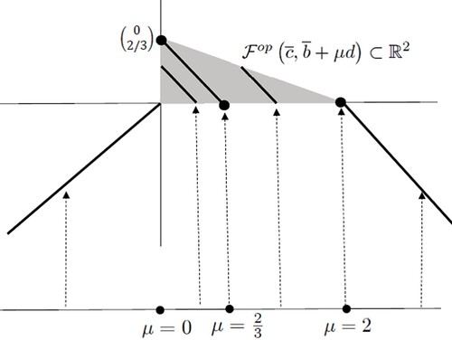
Example 1.1

Let us consider the problem in ${\mathbb{R}}^2$ (4) $\begin{array}{ll}\mathrm{m}\mathrm{i}\mathrm{n}\mathrm{i}\mathrm{m}\mathrm{i}\mathrm{z}\mathrm{e}& c_1{x}_1+c_2{x}_2\\ \mathrm{s}\mathrm{u}\mathrm{b}\mathrm{j}\mathrm{e}\mathrm{c}\mathrm{t}\mathrm{t}\mathrm{o}& x_1\le b_1,x_2\le b_2,x_1+x_2\le b_3,-\frac{1}{2}{x}_1+\frac{1}{2}{x}_2\le b_4,\end{array}$(4) with $c=\overline{c}=(\genfrac{}{}{0ex}{}{-1}{-1})\mathrm{a}\mathrm{n}\mathrm{d}b={(0,0,0,1)}^{\mathrm{\prime }}+\mu {(1,1,1,-1)}^{\mathrm{\prime }},\mu \in \mathbb{R};$in other words, we are perturbing $\overline{b}=(0,0,0,1{)}^{\mathrm{\prime }}$ in the directions $\pm d$ with $d=(1,1,1,-1{)}^{\mathrm{\prime }}$.

It can be easily checked that (see Figure 1) ${\mathcal{F}}^{op}(\overline{c},\overline{b}+\mu d)=\{\begin{array}{ll}\left\{{\displaystyle (\genfrac{}{}{0ex}{}{\mu }{\mu })}\right\}& \mathrm{i}\mathrm{f}\mu \le 0,\\ \mathrm{conv}\{{\displaystyle (\genfrac{}{}{0ex}{}{\mu }{0})},{\displaystyle (\genfrac{}{}{0ex}{}{0}{\mu })}\}& \mathrm{i}\mathrm{f}0\le \mu \le \frac{2}{3},\\ \mathrm{conv}\{{\displaystyle (\genfrac{}{}{0ex}{}{\mu }{0})},{\displaystyle (\genfrac{}{}{0ex}{}{-1+\frac{3}{2}\mu }{1-\frac{1}{2}\mu })}\}& \mathrm{i}\mathrm{f}\frac{2}{3}\le \mu \le 2,\\ \left\{{\displaystyle (\genfrac{}{}{0ex}{}{\mu }{2-\mu })}\right\}& \mathrm{i}\mathrm{f}\mu \ge 2.\end{array}$In particular $\left(\right(\overline{c},\overline{b}-d),{\displaystyle (\genfrac{}{}{0ex}{}{-1}{-1})})$ and $\left(\right(\overline{c},\overline{b}+d),{\displaystyle (\genfrac{}{}{0ex}{}{1}{0})})$ belong to $\mathrm{gph}{\mathcal{F}}^{op}$, while the middle point $\left(\right(\overline{c},\overline{b}),{\displaystyle (\genfrac{}{}{0ex}{}{0}{-1/2})})$ does not.

Figure 1. Local directional convexity in Example 1.1.

Now we summarize the structure of the paper. Section 2 contains some notation and preliminary results used later on. Section 3 formalizes the announced local directional convexity of $\mathrm{gph}{\mathcal{F}}^{op}$. The main result of this section, Theorem 3.1, is applied in Section 4 to establish Lemma 4.1, which constitutes a key step in the process of computing $\mathrm{Lipusc}{\mathcal{F}}^{op}\left(\overline{\pi }\right)$, leading to Theorem 4.2. Finally, Section 5 includes some conclusions and perspectives. In particular, the so-called Hoffman stability modulus is recalled, which is known to coincide with the Lipschitz upper semicontinuity modulus under the convexity of the graph. This is the case of $\mathcal{F}$, but no longer of ${\mathcal{F}}^{op}$ (see Example 5.1). The reader is referred to [3, 14–18] for extra details about Hoffman constants from a global (instead of semi-local) approach.

2. Preliminaries

This section introduces some necessary notation and results which are used later on. Given $X\subset {\mathbb{R}}^p$, $p\in \mathbb{N}$, we use the standard notation $\mathrm{c}\mathrm{o}\mathrm{n}\mathrm{e}X$ and $\mathrm{s}\mathrm{p}\mathrm{a}\mathrm{n}X$ for the conical convex hull and linear hull of X respectively, with the convention $\mathrm{cone}set=\mathrm{span}set=\left\{0_p\right\}$ (the zero vector of ${\mathbb{R}}^p$). Provided that X is convex, $\mathrm{e}\mathrm{x}\mathrm{t}\mathrm{r}X$ stands for the set of extreme points of X.

Consider a generic multifunction $\mathcal{M}:Y\rightrightarrows X$ between metric spaces Y and X (with both distances denoted by d). Recall that the graph and the domain of $\mathcal{M}$ are respectively given by $(y,x)\in \mathrm{gph}\mathcal{M}\iff x\in \mathcal{M}\left(y\right)$ and $y\in \mathrm{dom}\mathcal{M}\iff \mathcal{M}\left(y\right)\ne set$. Mapping $\mathcal{M}$ is said to be calm at $(\overline{y},\overline{x})\in \mathrm{gph}\mathcal{M}$ if there exist a constant $\kappa \ge 0$ and neighbourhoods V of $\overline{y}$ and U of $\overline{x}$ such that (5) $\mathrm{d}(x,\mathcal{M}(\overline{y}\left)\right)\le \kappa \mathrm{d}(y,\overline{y})\mathrm{f}\mathrm{o}\mathrm{r}\mathrm{a}\mathrm{l}\mathrm{l}y\in V\mathrm{a}\mathrm{n}\mathrm{d}\mathrm{a}\mathrm{l}\mathrm{l}x\in \mathcal{M}\left(y\right)\cap U,$(5) where $\mathrm{d}(x,\mathrm{\Omega }):=inf\left\{\mathrm{d}\right(x,\omega ):\omega \in \mathrm{\Omega }\}$, provided that $x\in X$ and $\mathrm{\Omega }\subset X$, with the usual convention $infset:=+\mathrm{\infty }$ and $\mathrm{d}(x,set)=+\mathrm{\infty }$. Since we are concerned with nonnegative constants, we understand that $supset:=0$. It is well-known (see, e.g. [4, Theorem 3H.3 and Exercise 3H.4]) that neighbourhood V appearing in the definition of calmness is redundant; formally, the calmness of $\mathcal{M}$ at $(\overline{y},\overline{x})\in \mathrm{gph}\mathcal{M}$ is equivalent to the existence of a constant $\kappa \ge 0$ and a (possibly smaller) neighbourhood U of $\overline{x}$ such that (6) $\mathrm{d}(x,\mathcal{M}(\overline{y}\left)\right)\le \kappa \mathrm{d}(\overline{y},{\mathcal{M}}^{-1}(x\left)\right)\mathrm{f}\mathrm{o}\mathrm{r}\mathrm{a}\mathrm{l}\mathrm{l}x\in U.$(6) The latter property is known as the metric subregularity of ${\mathcal{M}}^{-1}$ at $(\overline{x},\overline{y})$ (recall that $y\in {\mathcal{M}}^{-1}\left(x\right)\iff x\in \mathcal{M}\left(y\right))$. The calmness modulus of $\mathcal{M}$ at $(\overline{y},\overline{x})\in \mathrm{gph}\mathcal{M}$, denoted by $\mathrm{clm}\mathcal{M}(\overline{y},\overline{x})$, is the infimum of constants κ such that (5(5) $\mathrm{d}(x,\mathcal{M}(\overline{y}\left)\right)\le \kappa \mathrm{d}(y,\overline{y})\mathrm{f}\mathrm{o}\mathrm{r}\mathrm{a}\mathrm{l}\mathrm{l}y\in V\mathrm{a}\mathrm{n}\mathrm{d}\mathrm{a}\mathrm{l}\mathrm{l}x\in \mathcal{M}\left(y\right)\cap U,$(5) ) (equivalently (6(6) $\mathrm{d}(x,\mathcal{M}(\overline{y}\left)\right)\le \kappa \mathrm{d}(\overline{y},{\mathcal{M}}^{-1}(x\left)\right)\mathrm{f}\mathrm{o}\mathrm{r}\mathrm{a}\mathrm{l}\mathrm{l}x\in U.$(6) )) holds for some associated neighbourhoods; this modulus can be written as: (7) $\mathrm{clm}\mathcal{M}(\overline{y},\overline{x})=\underset{\begin{array}{c}(y,x)\to (\overline{y},\overline{x})\\ x\in \mathcal{M}\left(y\right)\end{array}}{lim sup}\frac{\mathrm{d}(x,\mathcal{M}(\overline{y}\left)\right)}{\mathrm{d}(y,\overline{y})}=\underset{x\to \overline{x}}{lim sup}\frac{\mathrm{d}(x,\mathcal{M}(\overline{y}\left)\right)}{\mathrm{d}(\overline{y},{\mathcal{M}}^{-1}(x\left)\right)},$(7) where $\frac{0}{0}:=0$ and $limsup$ is understood as the supremum (maximum, indeed) of all possible sequential upper limits (i.e. with $(y,x)$ being replaced with elements of sequences $\left\{\right(y_r,x_r){\}}_{r\in \mathbb{N}}$ converging to $(\overline{y},\overline{x})$ as $r\to \mathrm{\infty }$).

2.1. Lipschitz upper semicontinuity of multifunctions

The current work is focussed on a semi-local Lipschitz-type property: A multifunction $\mathcal{M}$ is said to be Lipschitz upper semicontinuous (see, e.g. [[1, Definition 2.1(iii)],[3, Section 3]]) at $\overline{y}\in \mathrm{dom}\mathcal{M}$ if there exist a constant $\kappa \ge 0$ and a neighbourhood V of $\overline{y}$ such that (8) $\mathrm{d}(x,\mathcal{M}(\overline{y}\left)\right)\le \kappa \mathrm{d}(y,\overline{y})\mathrm{f}\mathrm{o}\mathrm{r}\mathrm{a}\mathrm{l}\mathrm{l}y\in V\mathrm{a}\mathrm{n}\mathrm{d}\mathrm{a}\mathrm{l}\mathrm{l}x\in \mathcal{M}\left(y\right).$(8) The associated Lipschitz upper semicontinuity modulus at $\overline{y}\in \mathrm{dom}\mathcal{M}$, denoted by $\mathrm{Lipusc}\mathcal{M}\left(\overline{y}\right)$, is defined as the infimum of constants κ satisfying (8(8) $\mathrm{d}(x,\mathcal{M}(\overline{y}\left)\right)\le \kappa \mathrm{d}(y,\overline{y})\mathrm{f}\mathrm{o}\mathrm{r}\mathrm{a}\mathrm{l}\mathrm{l}y\in V\mathrm{a}\mathrm{n}\mathrm{d}\mathrm{a}\mathrm{l}\mathrm{l}x\in \mathcal{M}\left(y\right).$(8) ) for some associated V. Clearly V is not redundant here. The following result provides a limiting expression for $\mathrm{Lipusc}\mathcal{M}\left(\overline{y}\right)$.

Proposition 2.1

[3, Proposition 2(i)]

Let $\mathcal{M}:Y\rightrightarrows X$ be a multifunction between metric spaces and let $\overline{y}\in \mathrm{dom}\mathcal{M}$, then $\mathrm{Lipusc}\mathcal{M}\left(\overline{y}\right)=\underset{y\to \overline{y}}{lim sup}\left(\underset{x\in \mathcal{M}\left(y\right)}{sup}\frac{\mathrm{d}(x,\mathcal{M}(\overline{y}\left)\right)}{\mathrm{d}(y,\overline{y})}\right).$

The following result establishes the relationship between calmness and Lipschitz upper semicontinuity for generic multifunctions. See Section 5 for additional comments including the so-called Hoffman stability, defined in (22(22) $\mathrm{d}(x,\mathcal{M}(\overline{y}\left)\right)\le \kappa \mathrm{d}(\overline{y},{\mathcal{M}}^{-1}(x\left)\right)\mathrm{f}\mathrm{o}\mathrm{r}\mathrm{a}\mathrm{l}\mathrm{l}x\in X.$(22) ).

Theorem 2.1

[3, Corollary 2 and Theorem 4]

Let $\mathcal{M}:Y\rightrightarrows X$ be a multifunction between metric spaces and let $\overline{y}\in \mathrm{dom}\mathcal{M}$. We have (9) $\mathrm{Lipusc}\mathcal{M}\left(\overline{y}\right)\ge \underset{x\in \mathcal{M}\left(\overline{y}\right)}{sup}\mathrm{clm}\mathcal{M}(\overline{y},x).$(9) Moreover, equality holds in (9(9) $\mathrm{Lipusc}\mathcal{M}\left(\overline{y}\right)\ge \underset{x\in \mathcal{M}\left(\overline{y}\right)}{sup}\mathrm{clm}\mathcal{M}(\overline{y},x).$(9) ) if Y is a normed space, X is a reflexive Banach space, $\mathrm{gph}\mathcal{M}$ is a nonempty convex set, and $\mathcal{M}\left(\overline{y}\right)$ is closed.

Remark 2.1

1. Observe that the previous theorem relates local and semi-local Lipschitz-type measures for multifunctions.

2. The convexity assumption in the previous theorem is not superfluous for establishing equality in (9(9) $\mathrm{Lipusc}\mathcal{M}\left(\overline{y}\right)\ge \underset{x\in \mathcal{M}\left(\overline{y}\right)}{sup}\mathrm{clm}\mathcal{M}(\overline{y},x).$(9) ), as it was shown in [3, Example 2].

2.2. Lipschitz upper semicontinuity of the feasible set mapping

This subsection deals with the feasible set mapping $\mathcal{F}:{\mathbb{R}}^m\rightrightarrows {\mathbb{R}}^n$ introduced in (2(2) $\begin{array}{rl}\mathcal{F}\left(b\right)& :=\{x\in {\mathbb{R}}^n:a_t^{\mathrm{\prime }}x\le b_t\mathrm{f}\mathrm{o}\mathrm{r}\mathrm{a}\mathrm{l}\mathrm{l}t\in T\},\end{array}$(2) ), which has a closed convex graph and, so, Theorem 2.1 allows us to write (10) $\mathrm{Lipusc}\mathcal{F}\left(\overline{b}\right)=\underset{x\in \mathcal{F}\left(\overline{b}\right)}{sup}\mathrm{clm}\mathcal{F}(\overline{b},x).$(10) Going further, the next theorem provides a more computable expression for $\mathrm{Lipusc}\mathcal{F}\left(\overline{b}\right)$ as far as it involves a finite amount of calmness moduli. It appeals to the following set of extreme points: (11) $\mathcal{E}\left(b\right):=\mathrm{extr}\left(\mathcal{F}\right(b)\cap \mathrm{span}\{a_t,t\in T\}),b\in \mathrm{dom}\mathcal{F}.$(11) For details about this construction the reader is addressed to [19, p. 142]. In addition to the following theorem, set $\mathcal{E}\left(b\right)$ is also a key tool in [20] to provide a point-based formula for the calmness modulus of the optimal value function in linear optimization. This set is known to be always nonempty and finite.

Theorem 2.2

[3, See Theorems 4 and 6]

Let $\overline{b}\in \mathrm{dom}\mathcal{F}$. Then (12) $\mathrm{Lipusc}\mathcal{F}\left(\overline{b}\right)=\underset{x\in \mathcal{E}\left(\overline{b}\right)}{max}\mathrm{clm}\mathcal{F}(\overline{b},x).$(12)

In the sequel, for any $(b,x)\in \mathrm{gph}\mathcal{F}$, $T_b\left(x\right)$ represents the set of active indices at x, defined as $T_b\left(x\right):=\{t\in T:a_t^{\mathrm{\prime }}x=b_t\}.$In particular, it is appealed to in the definition of the following family of sets appearing in the next remark: given $(b,x)\in \mathrm{gph}\mathcal{F}$, ${\mathcal{D}}_b\left(x\right)$ is formed by all subsets $D\subset T_b\left(x\right)$ such that system $\left\{\begin{array}{rl}{a}_t^{\mathrm{\prime }}d=1,& t\in D,\\ a_t^{\mathrm{\prime }}d<1,& t\in T_b\left(x\right)\setminus D\end{array}\right\}$is consistent (in the variable $d\in {\mathbb{R}}^n);$ in other words, $\{a_t$, $t\in D\}$ lives in some hyperplane which leaves the remaining coefficient vectors $a_t,t\in T_b\left(x\right)\setminus D$ and the origin, $0_n$, in one of its two associated open half-spaces.

Remark 2.2

It is worth mentioning that any calmness modulus, $\mathrm{clm}\mathcal{F}(\overline{b},x)$, at any $x\in \mathcal{E}\left(\overline{b}\right)$ appearing in (12(12) $\mathrm{Lipusc}\mathcal{F}\left(\overline{b}\right)=\underset{x\in \mathcal{E}\left(\overline{b}\right)}{max}\mathrm{clm}\mathcal{F}(\overline{b},x).$(12) ) can be computed through the point-based formula given in [2, Theorem 4] (see also [3, Theorem 3], as stated in the introduction), which is recalled here for completeness: (13) $\mathrm{c}\mathrm{l}\mathrm{m}\mathcal{F}(\overline{b},\overline{x})=\underset{D\in {\mathcal{D}}_{\overline{b}}\left(\overline{x}\right)}{max}{d}_{\ast }{(0_n,\mathrm{c}\mathrm{o}\mathrm{n}\mathrm{v}\{a_t,t\in D\})}^{-1},(\overline{b},\overline{x})\in \mathrm{g}\mathrm{p}\mathrm{h}\mathcal{F},$(13) where $d_{\ast }$ represents the distance associated with the dual norm $\Vert \cdot {\Vert }_{\ast }$.

Remark 2.3

The fact of considering RHS perturbations is crucial in our analysis. Observe that in the case when the $a_t$'s are also perturbed the corresponding feasible set mapping is no longer Lipschitz upper semicontinuous in general. Just consider the example in ${\mathbb{R}}^2$ with only one constraint: $\tilde{\mathcal{F}}(a,b)=\{x\in {\mathbb{R}}^2\mid a_1{x}_1+a_2{x}_2\le b\},a=(a_1,a_2{)}^{\mathrm{\prime }}\in {\mathbb{R}}^2,b\in \mathbb{R}$. Then, for each $r=1,2,\dots$, we have $\underset{x\in \tilde{\mathcal{F}}((1,-\frac{1}{r}),0)}{sup}\frac{\mathrm{d}(x,\tilde{\mathcal{F}}({(1,0)}^{\mathrm{\prime }},0\left)\right)}{r^{-1}}\ge \underset{k\to \mathrm{\infty }}{lim}\frac{\mathrm{d}((\genfrac{}{}{0ex}{}{k}{rk}),\tilde{\mathcal{F}}\left(\right(1,0{)}^{\mathrm{\prime }},0))}{r^{-1}}=+\mathrm{\infty },$which entails $\mathrm{Lipusc}\tilde{\mathcal{F}}\left(\right(1,0{)}^{\mathrm{\prime }},0)=+\mathrm{\infty }$. Roughly speaking, the previous situation arises from the semi-local nature of this property (i.e. the fact that it involves the whole feasible sets associated with perturbed parameters). Indeed, other variational properties of local character (dealing with parameters and points near the nominal ones) do not change so drastically. For instance, this is the case of the calmness property (see, [2, Theorem 5]).

3. Local directional convexity of ${\mathcal{F}}^{op}$

This is an instrumental section oriented to tackle our problem of computing $\mathrm{Lipusc}{\mathcal{F}}^{op}\left(\overline{\pi }\right)$. As $\mathrm{gph}{\mathcal{F}}^{op}$ is not convex, we are not allowed to apply the last part of Theorem 2.1, and this fact entails notable differences with respect to the methodology followed in [3]. Specifically, this section is devoted to establish a certain directional-type convexity of the graph of ${\mathcal{F}}^{op}$ around $\overline{b}$ with a fixed $\overline{c}$, where only local directional RHS perturbations of the constraints are considered; see Figure 1 for a geometrical motivation. Formally, associated with our nominal problem $\overline{\pi }=(\overline{c},\overline{b})$, any scalar $ϵ>0$, and any direction $d\in {\mathbb{R}}^m$ with $\Vert d{\Vert }_{\mathrm{\infty }}=1$, we consider the local directional optimal set mapping ${\mathcal{F}}_{\overline{\pi },d,ϵ}^{op}:[0,ϵ]\rightrightarrows {\mathbb{R}}^n$ given by (14) ${\mathcal{F}}_{\overline{\pi },d,ϵ}^{op}\left(\mu \right)={\mathcal{F}}^{op}(\overline{c},\overline{b}+\mu d),\mu \in [0,ϵ].$(14) The following lemmas constitute key tools for establishing Theorem 3.1. To start with, we introduce some extra notation: given $\pi =(c,b)\in \mathrm{dom}{\mathcal{F}}^{op}$, ${\mathcal{M}}_{\pi }$ denotes the so-called minimal KKT subsets of indices at π, defined as (15) ${\mathcal{M}}_{\pi }:=\{D\subset T_b\left(x\right)|\begin{array}{l}-c\in \mathrm{cone}\{a_t,t\in D\}\\ D\mathrm{i}\mathrm{s}\mathrm{m}\mathrm{i}\mathrm{n}\mathrm{i}\mathrm{m}\mathrm{a}\mathrm{l}\mathrm{f}\mathrm{o}\mathrm{r}\mathrm{t}\mathrm{h}\mathrm{e}\mathrm{i}\mathrm{n}\mathrm{c}\mathrm{l}\mathrm{u}\mathrm{s}\mathrm{i}\mathrm{o}\mathrm{n}\mathrm{o}\mathrm{r}\mathrm{d}\mathrm{e}\mathrm{r}\end{array}\},$(15) provided that x is any optimal point of π. For convenience, sometimes ${\mathcal{M}}_{\pi }$ is alternatively denoted by ${\mathcal{M}}_{c,b}$ for $\pi =(c,b)\in \mathrm{dom}{\mathcal{F}}^{op}$. Let us observe that ${\mathcal{M}}_{\pi }$ is correctly defined since the expression in (15(15) ${\mathcal{M}}_{\pi }:=\{D\subset T_b\left(x\right)|\begin{array}{l}-c\in \mathrm{cone}\{a_t,t\in D\}\\ D\mathrm{i}\mathrm{s}\mathrm{m}\mathrm{i}\mathrm{n}\mathrm{i}\mathrm{m}\mathrm{a}\mathrm{l}\mathrm{f}\mathrm{o}\mathrm{r}\mathrm{t}\mathrm{h}\mathrm{e}\mathrm{i}\mathrm{n}\mathrm{c}\mathrm{l}\mathrm{u}\mathrm{s}\mathrm{i}\mathrm{o}\mathrm{n}\mathrm{o}\mathrm{r}\mathrm{d}\mathrm{e}\mathrm{r}\end{array}\},$(15) ) indeed does not depend on x as it was commented in [20, Remark 2]. Finally, we introduce the counterpart of $\mathcal{E}\left(b\right)$ when dealing with optimization problems, (16) ${\mathcal{E}}^{op}\left(\pi \right):=\mathrm{extr}\left({\mathcal{F}}^{op}\right(\pi )\cap \mathrm{span}\{a_t,t\in T\}),\pi \in \mathrm{dom}{\mathcal{F}}^{op}.$(16) The reader is referred to [20, Section 2.2] for additional details about this set of extreme points. Standard arguments of linear optimization yield ${\mathcal{E}}^{op}\left(\pi \right)={\mathcal{F}}^{op}\left(\pi \right)\cap \mathcal{E}\left(b\right)$ for $\pi =(c,b)\in \mathrm{dom}{\mathcal{F}}^{op}$.

Lemma 3.1

[20, Lemma 2]

Let $\{{\pi }^r{\}}_{r\in \mathbb{N}}\subset \mathrm{dom}{\mathcal{F}}^{op}$ converge to $\overline{\pi }$. Then $set\ne {\mathrm{Lim\; sup}}_r{\mathcal{E}}^{op}\left({\pi }^r\right)\subset {\mathcal{E}}^{op}\left(\overline{\pi }\right),$where ${\mathrm{Lim\; sup}}_r$ stands for the Painlevé–Kuratowski upper/outer limit as $r\to \mathrm{\infty }$ (see, e.g. [6, 7]).

Lemma 3.2

Let $(\overline{c},\overline{b})\in \mathrm{dom}{\mathcal{F}}^{op}$. Then there exists $ϵ>0$ such that for every $b\in \mathrm{dom}\mathcal{F}$ with $\Vert b-\overline{b}{\Vert }_{\mathrm{\infty }}\le ϵ$ we have ${\mathcal{M}}_{\overline{c},b}\subset {\mathcal{M}}_{\overline{c},\overline{b}}$.

Proof.

Reasoning by contradiction, suppose that there exists a sequence $\{b^r{\}}_{r\in \mathbb{N}}$ such that $\mathrm{dom}\mathcal{F}\ni b^r\to \overline{b}$ and $D_r\in {\mathcal{M}}_{\overline{c},b^r}\setminus {\mathcal{M}}_{\overline{c},\overline{b}}$ for all $r\in \mathbb{N}$. Since $D_r\subset T$ (finite) for all r, we may assume (by taking a subsequence if necessary) that $\{D_r{\}}_{r\in \mathbb{N}}$ is constant, say $D_r=D$ for all r.

Applying Lemma 3.1, let $\overline{x}\in {\mathrm{Lim\; sup}}_r{\mathcal{E}}^{op}(\overline{c},b^r)$ and, without loss of generality (for an appropriate subsequence, without relabelling), write $\overline{x}=\underset{r}{lim}{x}^r$, for some $x^r\in {\mathcal{E}}^{op}(\overline{c},b^r)$, $r=1,2,\dots$ For each r, $D\in {\mathcal{M}}_{\overline{c},b^r}$ entails $D\subset T_{b^r}\left(x^r\right)$, which yields $D\subset T_{\overline{b}}\left(\overline{x}\right)$. Moreover, $-\overline{c}\in \mathrm{cone}\{a_t,t\in D\}$ and D is minimal with respect to this property since it is for any r (recall $D_r=D$). Hence, we attain the contradiction $D\in {\mathcal{M}}_{\overline{c},\overline{b}}$.

Theorem 3.1

Let $\overline{\pi }=(\overline{c},\overline{b})\in \mathrm{dom}{\mathcal{F}}^{op}$ and $ϵ>0$ be as in Lemma 3.2. Then $\mathrm{gph}{\mathcal{F}}_{\overline{\pi },d,ϵ}^{op}$ is convex for all $d\in {\mathbb{R}}^m$ with $\Vert d{\Vert }_{\mathrm{\infty }}=1$.

Proof.

Let $({\mu }_0,x^0)$, $({\mu }_1,x^1)\in \mathrm{gph}{\mathcal{F}}_{\overline{\pi },d,ϵ}^{op}$ with $0\le {\mu }_0\le {\mu }_1\le ϵ$. Let us see that $({\mu }_{\lambda },x^{\lambda }):=(1-\lambda )({\mu }_0,x^0)+\lambda ({\mu }_1,x^1)\in \mathrm{gph}{\mathcal{F}}_{\overline{\pi },d,ϵ}^{op}$ for $\lambda \in ]0,1[$. If ${\mu }_0={\mu }_1$, then $x^0$ and $x^1$ belong to the same convex set ${\mathcal{F}}^{op}(\overline{c},\overline{b}+{\mu }_{0}d)$, and hence clearly $x^{\lambda }\in {\mathcal{F}}^{op}(\overline{c},\overline{b}+{\mu }_{0}d)={\mathcal{F}}_{\overline{\pi },d,ϵ}^{op}\left({\mu }_{\lambda }\right)$for all $\lambda \in ]0,1[$.

From now on, let us assume ${\mu }_0<{\mu }_1$. First observe that $x^{\lambda }\in \mathcal{F}(\overline{b}+{\mu }_{\lambda }d)$ for all $\lambda \in ]0,1[$ because of the convexity of $\mathrm{gph}\mathcal{F}$. We distinguish two cases:

Case 1 ${\mu }_0=0$. Fix any $\lambda \in ]0,1[$. Observe that in this case ${\mu }_{\lambda }=\lambda {\mu }_1$. Let us prove that $x^{\lambda }\in {\mathcal{F}}_{\overline{\pi },d,ϵ}^{op}\left({\mu }_{\lambda }\right)$. Take $D_1\in {\mathcal{M}}_{\overline{c},\overline{b}+{\mu }_{1}d}\subset {\mathcal{M}}_{\overline{c},\overline{b}}$ (because of Lemma 3.2 and the choice of ε). In particular, $D_1\subset T_{\overline{b}+{\mu }_{1}d}\left(x^1\right)\cap T_{\overline{b}}\left(x^0\right)$. Therefore $D_1\subset T_{\overline{b}+\lambda {\mu }_{1}d}\left(x^{\lambda }\right)$ since, for any $t\in D_1$, $a_t^{\mathrm{\prime }}{x}^{\lambda }=(1-\lambda )a_t^{\mathrm{\prime }}{x}^0+\lambda a_t^{\mathrm{\prime }}{x}^1=(1-\lambda ){\overline{b}}_t+\lambda ({\overline{b}}_t+{\mu }_1{d}_t)={\overline{b}}_t+\lambda {\mu }_1{d}_t.$Hence, as we are not perturbing $\overline{c}$, KKT optimality conditions ensure $x^{\lambda }\in {\mathcal{F}}^{op}(\overline{c},\overline{b}+\lambda {\mu }_{1}d)={\mathcal{F}}_{\overline{\pi },d,ϵ}^{op}\left({\mu }_{\lambda }\right)$.

Case 2 ${\mu }_0>0$. Fix again any $\lambda \in ]0,1[$ and let us see that $x^{\lambda }\in {\mathcal{F}}_{\overline{\pi },d,ϵ}^{op}\left({\mu }_{\lambda }\right)$.

Start by choosing an arbitrary $\overline{x}\in {\mathcal{F}}_{\overline{\pi },d,ϵ}^{op}\left(0\right)={\mathcal{F}}^{op}(\overline{c},\overline{b})$ and define ${\tilde{x}}^1:=(1-\frac{{\mu }_0}{{\mu }_1})\overline{x}+\frac{{\mu }_0}{{\mu }_1}{x}^1.$Reasoning as in the previous case, with $\overline{x}$ and $\frac{{\mu }_0}{{\mu }_1}$ playing the role of $x^0$ and λ, respectively, we deduce ${\tilde{x}}^1\in {\mathcal{F}}_{\overline{\pi },d,ϵ}^{op}\left(\frac{{\mu }_0}{{\mu }_1}{\mu }_1\right)={\mathcal{F}}_{\overline{\pi },d,ϵ}^{op}\left({\mu }_0\right).$Appealing to the convexity of the previous optimal set, define ${\tilde{x}}^{\alpha }:=(1-\alpha )x^0+\alpha {\tilde{x}}^1\in {\mathcal{F}}_{\overline{\pi },d,ϵ}^{op}\left({\mu }_0\right)\mathrm{\forall }\alpha \in [0,1].$A routine computation yields the existence of scalars $\alpha \in [0,1]$ and $\text{β}\ge 1$ such that $x^{\lambda }-\overline{x}=\text{β}({\tilde{x}}^{\alpha }-\overline{x}).$Indeed, they are unique and their explicit expressions are $\alpha =\frac{\lambda {\mu }_1}{(1-\lambda ){\mu }_0+\lambda {\mu }_1},\text{β}=\frac{(1-\lambda ){\mu }_0+\lambda {\mu }_1}{{\mu }_0}.$Since ${\tilde{x}}^{\alpha }\in {\mathcal{F}}_{\overline{\pi },d,ϵ}^{op}\left({\mu }_0\right)$, there exists $D_{\alpha }\in {\mathcal{M}}_{\overline{c},\overline{b}+{\mu }_{0}d}\subset {\mathcal{M}}_{\overline{c},\overline{b}}$, in particular, $D_{\alpha }\subset T_{\overline{b}+{\mu }_{0}d}\left({\tilde{x}}^{\alpha }\right)\cap T_{\overline{b}}\left(\overline{x}\right)$. Hence, for any $t\in D_{\alpha }$, taking into account the fact that $\text{β}{\mu }_0={\mu }_{\lambda }$, one has $\begin{array}{rl}{a}_t^{\mathrm{\prime }}{x}^{\lambda }& =a_t^{\mathrm{\prime }}\overline{x}+\text{β}{a}_t^{\mathrm{\prime }}({\tilde{x}}^{\alpha }-\overline{x})\\ & ={\overline{b}}_t+\text{β}({\overline{b}}_t+{\mu }_0{d}_t-{\overline{b}}_t)={\overline{b}}_t+\text{β}{\mu }_0{d}_t={\overline{b}}_t+{\mu }_{\lambda }{d}_t.\end{array}$In this way, $D_{\alpha }\subset T_{\overline{b}+{\mu }_{\lambda }d}\left(x^{\lambda }\right)$ and again the KKT optimality conditions yield $x^{\lambda }\in {\mathcal{F}}^{op}(\overline{c},\overline{b}+{\mu }_{\lambda }d)$. In other words, $({\mu }_{\lambda },x^{\lambda })\in \mathrm{gph}{\mathcal{F}}_{\overline{\pi },d,ϵ}^{op}$.

The following example illustrates the previous results.

Example 3.1

Example 1.1 revisited

Let us consider the parameterized problem (4(4) $\begin{array}{ll}\mathrm{m}\mathrm{i}\mathrm{n}\mathrm{i}\mathrm{m}\mathrm{i}\mathrm{z}\mathrm{e}& c_1{x}_1+c_2{x}_2\\ \mathrm{s}\mathrm{u}\mathrm{b}\mathrm{j}\mathrm{e}\mathrm{c}\mathrm{t}\mathrm{t}\mathrm{o}& x_1\le b_1,x_2\le b_2,x_1+x_2\le b_3,-\frac{1}{2}{x}_1+\frac{1}{2}{x}_2\le b_4,\end{array}$(4) ) in ${\mathbb{R}}^2$ with $T=\{1,2,3,4\}$ and let us see that the statement of Lemma 3.2 fulfils by taking $0<ϵ<\frac{2}{5}$. First observe that (17) $\begin{array}{c}\Vert b-\overline{b}{\Vert }_{\mathrm{\infty }}<\frac{2}{5}\\ x\in {\mathcal{F}}^{op}(\overline{c},b)\end{array}\}⟹T_b\left(x\right)\subset \{1,2,3\}.$(17) Reasoning by contradiction, assume that there exists $(b,x)\in {\mathbb{R}}^4\times {\mathbb{R}}^2$ such that $x\in {\mathcal{F}}^{op}(\overline{c},b)$, $\Vert b-\overline{b}{\Vert }_{\mathrm{\infty }}<\frac{2}{5}$ and $4\in T_b\left(x\right)$. It is clear that $\left\{4\right\}⫋T_b\left(x\right)$ according to KKT conditions ($-\overline{c}\notin \mathrm{cone}\left\{a_4\right\}$). Then, by distinguishing cases we attain a contradiction: assume that $1\in T_b\left(x\right)$, then $x_1=b_1$ and $-\frac{1}{2}{x}_1+\frac{1}{2}{x}_2=b_4$, which yields $x_2=b_1+2b_4>-\frac{2}{5}+2(1-\frac{2}{5})=\frac{4}{5}$ which contradicts $x_2\le b_2<\frac{2}{5}$. Hence $1\notin T_b\left(x\right)$. Then, necessarily $3\in T_b\left(x\right)$ (since $-\overline{c}\notin \mathrm{cone}\{a_2,a_4\})$, but again $x_1+x_2=b_3$ and $-\frac{1}{2}{x}_1+\frac{1}{2}{x}_2=b_4$ yield the contradiction $\frac{2}{5}>x_2=\frac{1}{2}{b}_3+b_4>-\frac{1}{5}+\frac{3}{5}=\frac{2}{5}$.

From (17(17) $\begin{array}{c}\Vert b-\overline{b}{\Vert }_{\mathrm{\infty }}<\frac{2}{5}\\ x\in {\mathcal{F}}^{op}(\overline{c},b)\end{array}\}⟹T_b\left(x\right)\subset \{1,2,3\}.$(17) ) one easily derives (18) ${\mathcal{M}}_{\overline{c},b}\subset {\mathcal{M}}_{\overline{c},\overline{b}}=\left\{\right\{1,2\},\{3\left\}\right\},\mathrm{w}\mathrm{h}\mathrm{e}\mathrm{n}\mathrm{e}\mathrm{v}\mathrm{e}\mathrm{r}\Vert b-\overline{b}{\Vert }_{\mathrm{\infty }}<\frac{2}{5}.$(18) Indeed, given any $\Vert b-\overline{b}{\Vert }_{\mathrm{\infty }}<\frac{2}{5}$ one can check ${\mathcal{M}}_{\overline{c},b}=\{\begin{array}{ll}\left\{\right\{1,2\},\{3\left\}\right\},& \mathrm{i}\mathrm{f}{b}_1+b_2=b_3,\\ \left\{\right\{1,2\left\}\right\},& \mathrm{i}\mathrm{f}{b}_1+b_2<b_3,\\ \left\{\right\{3\left\}\right\},& \mathrm{i}\mathrm{f}{b}_1+b_2>b_3.\end{array}$Therefore, for any $d\in {\mathbb{R}}^4$, with $\Vert d{\Vert }_{\mathrm{\infty }}=1$, and $\mu \in [0,\frac{2}{5}[$, we have (19) ${\mathcal{F}}^{op}(\overline{c},\overline{b}+\mu d)=\{\begin{array}{ll}\left\{\mu {\displaystyle (\genfrac{}{}{0ex}{}{d_1}{d_2})}\right\},& \mathrm{i}\mathrm{f}{d}_1+d_2\le d_3,\\ \mu \mathrm{conv}\{{\displaystyle (\genfrac{}{}{0ex}{}{d_1}{d_3-d_1})},{\displaystyle (\genfrac{}{}{0ex}{}{d_3-d_2}{d_2})}\},& \mathrm{i}\mathrm{f}{d}_1+d_2>d_3,\end{array}$(19) which clearly entails the convexity of $\mathrm{gph}{\mathcal{F}}_{\overline{\pi },d,ϵ}^{op}$ for each $d\in {\mathbb{R}}^4$ with $\Vert d{\Vert }_{\mathrm{\infty }}=1$ and each $0<ϵ<\frac{2}{5}$.

Finally, observe that (17(17) $\begin{array}{c}\Vert b-\overline{b}{\Vert }_{\mathrm{\infty }}<\frac{2}{5}\\ x\in {\mathcal{F}}^{op}(\overline{c},b)\end{array}\}⟹T_b\left(x\right)\subset \{1,2,3\}.$(17) ) is no longer true for $ϵ=\frac{2}{5}$ since $T_{\overline{b}+\frac{2}{5}{(-1,1,-1,-1)}^{\mathrm{\prime }}}\left({(-\frac{4}{5},\frac{2}{5})}^{\mathrm{\prime }}\right)=\{2,3,4\}.$However, (18(18) ${\mathcal{M}}_{\overline{c},b}\subset {\mathcal{M}}_{\overline{c},\overline{b}}=\left\{\right\{1,2\},\{3\left\}\right\},\mathrm{w}\mathrm{h}\mathrm{e}\mathrm{n}\mathrm{e}\mathrm{v}\mathrm{e}\mathrm{r}\Vert b-\overline{b}{\Vert }_{\mathrm{\infty }}<\frac{2}{5}.$(18) ) still holds by replacing $\frac{2}{5}$ with $\frac{1}{2}$, since the only way to preclude ${\mathcal{M}}_{\overline{c},b}\subset {\mathcal{M}}_{\overline{c},\overline{b}}$ is having $\{1,4\}\in {\mathcal{M}}_{\overline{c},b},$ which implies $\Vert b-\overline{b}{\Vert }_{\mathrm{\infty }}\ge \frac{1}{2}$; although the description of ${\mathcal{F}}^{op}(\overline{c},\overline{b}+\mu d)$ would be different from that of (19(19) ${\mathcal{F}}^{op}(\overline{c},\overline{b}+\mu d)=\{\begin{array}{ll}\left\{\mu {\displaystyle (\genfrac{}{}{0ex}{}{d_1}{d_2})}\right\},& \mathrm{i}\mathrm{f}{d}_1+d_2\le d_3,\\ \mu \mathrm{conv}\{{\displaystyle (\genfrac{}{}{0ex}{}{d_1}{d_3-d_1})},{\displaystyle (\genfrac{}{}{0ex}{}{d_3-d_2}{d_2})}\},& \mathrm{i}\mathrm{f}{d}_1+d_2>d_3,\end{array}$(19) ) when $\mu >\frac{2}{5}$.

4. Lipschitz upper semicontinuity of the optimal set mapping

This section tackles the final goal of the current paper: the computation of the Lipschitz upper semicontinuity modulus for the optimal set mapping ${\mathcal{F}}^{op}$ introduced in (3(3) $\begin{array}{rl}{\mathcal{F}}^{op}\left(\pi \right)& :=\arg min\{c^{\mathrm{\prime }}x:x\in \mathcal{F}\left(b\right)\}.\end{array}$(3) ). First, let us see that perturbations of c are redundant when looking for the aimed modulus. Formally, we consider ${\mathcal{F}}_{\overline{c}}^{op}:{\mathbb{R}}^m\rightrightarrows {\mathbb{R}}^n$ given by ${\mathcal{F}}_{\overline{c}}^{op}\left(b\right)={\mathcal{F}}^{op}(\overline{c},b),b\in {\mathbb{R}}^m.$

Proposition 4.1

[20, Lemma 4]

There exists $ϵ>0$ such that ${\mathcal{F}}^{op}\left(\pi \right)\subset {\mathcal{F}}^{op}(\overline{c},b),$whenever $\pi \equiv (c,b),\overline{\pi }\equiv (\overline{c},\overline{b})\in \mathrm{dom}{\mathcal{F}}^{op}$ satisfy $\Vert \pi -\overline{\pi }\Vert <ϵ$.

Corollary 4.1

Let $\overline{\pi }\equiv (\overline{c},\overline{b})\in \mathrm{dom}{\mathcal{F}}^{op}$. We have (20) $\mathrm{Lipusc}{\mathcal{F}}^{op}\left(\overline{\pi }\right)=\mathrm{Lipusc}{\mathcal{F}}_{\overline{c}}^{op}\left(\overline{b}\right)=\underset{b\to \overline{b}}{lim sup}\left(\underset{x\in {\mathcal{F}}^{op}(\overline{c},b)}{sup}\frac{\mathrm{d}(x,{\mathcal{F}}^{op}\left(\overline{\pi }\right))}{\mathrm{d}(b,\overline{b})}\right).$(20)

Proof.

Inequality $\mathrm{Lipusc}{\mathcal{F}}^{op}\left(\overline{\pi }\right)\ge \mathrm{Lipusc}{\mathcal{F}}_{\overline{c}}^{op}\left(\overline{b}\right)$ follows directly from the definitions. Appealing to Propositions 2.1 and 4.1 we have $\begin{array}{rl}\mathrm{Lipusc}{\mathcal{F}}^{op}\left(\overline{\pi }\right)& =\underset{\pi \to \overline{\pi }}{lim sup}\left(\underset{x\in {\mathcal{F}}^{op}\left(\pi \right)}{sup}\frac{\mathrm{d}(x,{\mathcal{F}}^{op}\left(\overline{\pi }\right))}{\mathrm{d}(\pi ,\overline{\pi })}\right)\\ & \le \underset{\pi \to \overline{\pi }}{lim sup}\left(\underset{x\in {\mathcal{F}}^{op}(\overline{c},b)}{sup}\frac{\mathrm{d}(x,{\mathcal{F}}^{op}\left(\overline{\pi }\right))}{\mathrm{d}(\pi ,\overline{\pi })}\right)\\ & \le \underset{b\to \overline{b}}{lim sup}\left(\underset{x\in {\mathcal{F}}^{op}(\overline{c},b)}{sup}\frac{\mathrm{d}(x,{\mathcal{F}}^{op}\left(\overline{\pi }\right))}{\mathrm{d}(b,\overline{b})}\right)\\ & =\mathrm{Lipusc}{\mathcal{F}}_{\overline{c}}^{op}\left(\overline{b}\right).\text{■}\end{array}$

From now on, appealing to the local directional convexity of the graph of ${\mathcal{F}}^{op}$ under RHS perturbations, we adapt some arguments used in [3] to the current setting. The following technical lemma uses Theorem 3.1 to provide an upper bound on the variation rate of optimal solutions with respect to RHS perturbations.

Lemma 4.1

Let $\overline{\pi }=(\overline{c},\overline{b})\in \mathrm{dom}{\mathcal{F}}^{op}$. Let $ϵ>0$ be as in Lemma 3.2, take $\left(\right(\overline{c},b),x)\in \mathrm{gph}{\mathcal{F}}^{op}$ with $\Vert b-\overline{b}{\Vert }_{\mathrm{\infty }}\le ϵ$ and let $p\left(x\right)$ be a projection (a best approximation) of x in ${\mathcal{F}}^{op}\left(\overline{\pi }\right)$. Then $\frac{\mathrm{d}(x,{\mathcal{F}}^{op}\left(\overline{\pi }\right))}{\mathrm{d}(b,\overline{b})}\le \mathrm{clm}{\mathcal{F}}^{op}(\overline{\pi },p\left(x\right)).$

Proof.

The case $b=\overline{b}$ is trivial from $0/0:=0$. Assume $b\ne \overline{b}$ and let $d:=\frac{b-\overline{b}}{\Vert b-\overline{b}{\Vert }_{\mathrm{\infty }}}$. With the notation (14(14) ${\mathcal{F}}_{\overline{\pi },d,ϵ}^{op}\left(\mu \right)={\mathcal{F}}^{op}(\overline{c},\overline{b}+\mu d),\mu \in [0,ϵ].$(14) ), $p\left(x\right)\in {\mathcal{F}}_{\overline{\pi },d,ϵ}^{op}\left(0\right)$ and $x\in {\mathcal{F}}_{\overline{\pi },d,ϵ}^{op}(\Vert b-\overline{b}{\Vert }_{\mathrm{\infty }})$, which entails, for each $\lambda \in [0,1]$, by applying Theorem 3.1, $x_{\lambda }:=(1-\lambda )p\left(x\right)+\lambda x\in {\mathcal{F}}_{\overline{\pi },d,ϵ}^{op}(\lambda \Vert b-\overline{b}{\Vert }_{\mathrm{\infty }})={\mathcal{F}}^{op}(\overline{c},(1-\lambda )\overline{b}+\lambda b).$Moreover, from [3, Lemma 1] we have that $p\left(x\right)$ is also a best approximation of $x_{\lambda }$ in ${\mathcal{F}}^{op}\left(\overline{\pi }\right);$ i.e. $\Vert x_{\lambda }-p\left(x\right)\Vert =\mathrm{d}(x_{\lambda },{\mathcal{F}}^{op}(\overline{\pi }\left)\right),$ $\lambda \in [0,1]$. Consequently, $\frac{\mathrm{d}(x_{\lambda },{\mathcal{F}}^{op}\left(\overline{\pi }\right))}{\Vert \lambda (b-\overline{b}){\Vert }_{\mathrm{\infty }}}=\frac{\lambda \Vert x-p\left(x\right)\Vert }{\lambda \Vert b-\overline{b}{\Vert }_{\mathrm{\infty }}}=\frac{\mathrm{d}(x,{\mathcal{F}}^{op}\left(\overline{\pi }\right))}{\mathrm{d}(b,\overline{b})},\mathrm{w}\mathrm{h}\mathrm{e}\mathrm{n}\mathrm{e}\mathrm{v}\mathrm{e}\mathrm{r}\lambda \in ]0,1].$Hence, letting $\lambda \to 0$ we obtain the aimed inequality.

Proposition 4.2

Let $\overline{\pi }=(\overline{c},\overline{b})\in \mathrm{dom}{\mathcal{F}}^{op}$, then $\mathrm{Lipusc}{\mathcal{F}}^{op}\left(\overline{\pi }\right)=\underset{z\in {\mathcal{F}}^{op}\left(\overline{\pi }\right)}{sup}\mathrm{clm}{\mathcal{F}}^{op}(\overline{\pi },z).$

Proof.

Inequality ‘$\ge$’ comes from Theorem 2.1. Let us prove the nontrivial inequality $\le$. Take an $ϵ>0$ as in Lemma 3.2 (and Theorem 3.1). We can write (recall Corollary 4.1) $\begin{array}{rl}\mathrm{Lipusc}{\mathcal{F}}^{op}(\overline{c},\overline{b})& =\underset{b\to \overline{b}}{lim sup}\left(\underset{x\in {\mathcal{F}}_{\overline{c}}^{op}\left(b\right)}{sup}\frac{\mathrm{d}(x,{\mathcal{F}}^{op}\left(\overline{\pi }\right))}{\mathrm{d}(b,\overline{b})}\right)\\ & \le \underset{\begin{array}{c}b\to \overline{b}\\ \Vert b-\overline{b}\Vert \le ϵ\end{array}}{lim sup}(\underset{x\in {\mathcal{F}}_{\overline{c}}^{op}\left(b\right)}{sup}\mathrm{clm}{\mathcal{F}}^{op}(\overline{\pi },p\left(x\right))),\end{array}$where we have applied Lemma 4.1 and, as in that lemma, for each $x\in {\mathcal{F}}_{\overline{c}}^{op}\left(b\right)$, with $\Vert b-\overline{b}\Vert \le ϵ$, $p\left(x\right)\in {\mathcal{F}}^{op}\left(\overline{\pi }\right)$ is a projection of x in ${\mathcal{F}}^{op}\left(\overline{\pi }\right)$.

Consequently, $\mathrm{Lipusc}{\mathcal{F}}^{op}\left(\overline{\pi }\right)\le \underset{z\in {\mathcal{F}}^{op}\left(\overline{\pi }\right)}{sup}\mathrm{clm}{\mathcal{F}}^{op}(\overline{\pi },z).$

Next we show that the supremum in the previous proposition may be reduced to a finite subset of points, indeed to points in ${\mathcal{E}}^{op}(\overline{c},\overline{b})$. To do that we appeal to the following theorem.

Theorem 4.1

[21, Corollary 4.1]

Let $(\overline{\pi },\overline{x})\in \mathrm{gph}{\mathcal{F}}^{op}$ with $\overline{\pi }=(\overline{c},\overline{b})$. Then (21) $\mathrm{clm}{\mathcal{F}}^{op}((\overline{c},\overline{b}),\overline{x})=\underset{D\in {\mathcal{M}}_{\overline{\pi }}}{max}\mathrm{clm}{\mathcal{L}}_D((\overline{b},-{\overline{b}}_D),\overline{x}),$(21) where, for each $D\in {\mathcal{M}}_{\overline{\pi }}$, ${\mathcal{L}}_D:{\mathbb{R}}^m\times {\mathbb{R}}^D\rightrightarrows {\mathbb{R}}^n$ is defined by ${\mathcal{L}}_D(b,d):=\{x\in {\mathbb{R}}^n:a_t^{\mathrm{\prime }}x\le b_t,t=1,\dots ,m;-a_t^{\mathrm{\prime }}x\le d_t,t\in D\},$and ${\overline{b}}_D:=({\overline{b}}_t{)}_{t\in D}$.

Remark 4.1

Observe that each ${\mathcal{L}}_D$ is nothing else but a feasible set mapping of the same type as $\mathcal{F}$ but associated with an enlarged system. Consequently, Remark 2.2 also applies here for computing each $\mathrm{clm}{\mathcal{L}}_D\left(\right(\overline{b},-{\overline{b}}_D),\overline{x})$, and therefore $\mathrm{clm}{\mathcal{F}}^{op}\left(\right(\overline{c},\overline{b}),\overline{x})$.

Finally, by gathering the previous results of this section, we can establish our main goal in the following theorem. We point out that this theorem provides an implementable procedure for computing the aimed $\mathrm{Lipusc}{\mathcal{F}}^{op}\left(\overline{\pi }\right)$ as far as it is written in terms of a finite amount of calmness moduli of feasible set mappings (as the previous theorem says) and these calmness moduli can be computed via formula (13(13) $\mathrm{c}\mathrm{l}\mathrm{m}\mathcal{F}(\overline{b},\overline{x})=\underset{D\in {\mathcal{D}}_{\overline{b}}\left(\overline{x}\right)}{max}{d}_{\ast }{(0_n,\mathrm{c}\mathrm{o}\mathrm{n}\mathrm{v}\{a_t,t\in D\})}^{-1},(\overline{b},\overline{x})\in \mathrm{g}\mathrm{p}\mathrm{h}\mathcal{F},$(13) ).

Theorem 4.2

Let $\overline{\pi }\in \mathrm{dom}{\mathcal{F}}^{op}$, then $\mathrm{Lipusc}{\mathcal{F}}^{op}\left(\overline{\pi }\right)=\underset{x\in {\mathcal{E}}^{op}\left(\overline{\pi }\right)}{max}\mathrm{clm}{\mathcal{F}}^{op}(\overline{\pi },x).$

Proof.

Starting from the equalities of Proposition 4.2 and Theorem 4.1, we can write $\begin{array}{rl}\mathrm{Lipusc}{\mathcal{F}}^{op}\left(\overline{\pi }\right)& =\underset{x\in {\mathcal{F}}^{op}\left(\overline{\pi }\right)}{sup}\mathrm{clm}{\mathcal{F}}^{op}(\overline{\pi },x)\\ & =\underset{x\in {\mathcal{F}}^{op}\left(\overline{\pi }\right)}{sup}\underset{D\in {\mathcal{M}}_{\overline{\pi }}}{max}\mathrm{clm}{\mathcal{L}}_D((\overline{b},-{\overline{b}}_D),x)\\ & =\underset{D\in {\mathcal{M}}_{\overline{\pi }}}{max}\underset{x\in {\mathcal{L}}_D(\overline{b},-{\overline{b}}_D)}{sup}\mathrm{clm}{\mathcal{L}}_D((\overline{b},-{\overline{b}}_D),x)\\ & =\underset{D\in {\mathcal{M}}_{\overline{\pi }}}{max}\underset{x\in {\mathcal{E}}^{op}\left(\overline{\pi }\right)}{max}\mathrm{clm}{\mathcal{L}}_D((\overline{b},-{\overline{b}}_D),x)\\ & =\underset{x\in {\mathcal{E}}^{op}\left(\overline{\pi }\right)}{max}\mathrm{clm}{\mathcal{F}}^{op}((\overline{c},\overline{b}),x).\end{array}$In the third equality we have used the fact that ${\mathcal{F}}^{op}(\overline{c},\overline{b})={\mathcal{L}}_D(\overline{b},-{\overline{b}}_D)$ for all $D\in {\mathcal{M}}_{\overline{\pi }}$ (see [21, Proposition 4.1]), while the fourth comes from Theorems 2.1 and 2.2 by taking Remark 4.1 into account, together with the fact that the role played by $\mathcal{E}\left(\overline{b}\right)$ in Theorem 2.2 is now played by $\mathrm{extr}({\mathcal{L}}_D(\overline{b},-{\overline{b}}_D)\cap \mathrm{span}\{a_t,t\in T\})={\mathcal{E}}^{op}\left(\overline{\pi }\right),\mathrm{f}\mathrm{o}\mathrm{r}\mathrm{a}\mathrm{l}\mathrm{l}D\in {\mathcal{M}}_{\overline{\pi }}.$The last equality comes again from Theorem 4.1.

5. Conclusions and perspectives

At this moment we recall the parallelism between both formulae of $\mathrm{Lipusc}\mathcal{F}\left(\overline{b}\right)$ and $\mathrm{Lipusc}{\mathcal{F}}^{op}\left(\overline{\pi }\right)$, for $\overline{\pi }=(\overline{c},\overline{b})\in \mathrm{dom}{\mathcal{F}}^{op}$, pointed out in Remark 1.1. The first one was established in [3] by strongly appealing to the convexity of $\mathrm{gph}\mathcal{F}$, while a local directional convexity property of $\mathrm{gph}{\mathcal{F}}^{op}$ has been used here to develop the second one. Indeed, [3] analyses another Lipschitz-type property, called there Hoffman stability, which is commented in the next subsection.

5.1. On the Hoffman stability of the optimal set

We say that $\mathcal{M}:Y\rightrightarrows X$, with Y and X being metric spaces, is Hoffman stable at $\overline{y}$ if there exists $\kappa \ge 0$ such that $\mathrm{d}(x,\mathcal{M}(\overline{y}\left)\right)\le \kappa \mathrm{d}(y,\overline{y})$ for all $y\in \mathrm{dom}\mathcal{M}$ and all $x\in \mathcal{M}\left(y\right)$, or, equivalently, if (22) $\mathrm{d}(x,\mathcal{M}(\overline{y}\left)\right)\le \kappa \mathrm{d}(\overline{y},{\mathcal{M}}^{-1}(x\left)\right)\mathrm{f}\mathrm{o}\mathrm{r}\mathrm{a}\mathrm{l}\mathrm{l}x\in X.$(22) The associated Hoffman modulus at $\overline{y}\in \mathrm{dom}\mathcal{M}$, $\mathrm{Hof}\mathcal{M}\left(\overline{y}\right)$, is the infimum of constants κ satisfying (22(22) $\mathrm{d}(x,\mathcal{M}(\overline{y}\left)\right)\le \kappa \mathrm{d}(\overline{y},{\mathcal{M}}^{-1}(x\left)\right)\mathrm{f}\mathrm{o}\mathrm{r}\mathrm{a}\mathrm{l}\mathrm{l}x\in X.$(22) ) and may be expressed as $\mathrm{Hof}\mathcal{M}\left(\overline{y}\right)=\underset{(y,x)\in \mathrm{gph}\mathcal{M}}{sup}\frac{\mathrm{d}(x,\mathcal{M}(\overline{y}\left)\right)}{\mathrm{d}(y,\overline{y})}=\underset{x\in X}{sup}\frac{\mathrm{d}(x,\mathcal{M}(\overline{y}\left)\right)}{\mathrm{d}(\overline{y},{\mathcal{M}}^{-1}(x\left)\right)}.$Theorem 4 in [3], again appealing to the convexity of $\mathrm{gph}\mathcal{F}$, establishes the equality $\mathrm{Lipusc}\mathcal{F}\left(\overline{b}\right)=\mathrm{Hof}\mathcal{F}\left(\overline{b}\right),$which is no longer true for our optimal set mapping ${\mathcal{F}}^{op}$, neither for ${\mathcal{F}}_{\overline{c}}^{op}$ (recall that $\mathrm{gph}{\mathcal{F}}^{op}$ and $\mathrm{gph}{\mathcal{F}}_{\overline{c}}^{op}$ are not convex), as the following example shows.

Example 5.1

Consider the parameterized problem of Example 1.1 with ${\mathbb{R}}^2$ being endowed with the Euclidean norm, and consider the following nominal parameters: $\overline{c}=(\genfrac{}{}{0ex}{}{-1}{-1})\mathrm{a}\mathrm{n}\mathrm{d}\overline{b}={(-1,-1,-1,1)}^{\mathrm{\prime }}.$The reader can easily check that $\Vert (c,b)-(\overline{c},\overline{b})\Vert <\frac{1}{3}\Rightarrow {\mathcal{F}}^{op}(c,b)=\left\{{\displaystyle (\genfrac{}{}{0ex}{}{b_1}{b_2})}\right\}.$Thus, an ad hoc routine calculation gives $\mathrm{Lipusc}{\mathcal{F}}^{op}(\overline{c},\overline{b})=\sqrt{2}.$Of course Theorem 4.2 can be alternatively used for this computation.

Now, let us perturb $\overline{b}$ by considering $b_{\mu }:=\overline{b}+\mu (-1,0,0,-1{)}^{\mathrm{\prime }}$ for $\mu \ge 2/3$. Then it is easy to check that ${\displaystyle (\genfrac{}{}{0ex}{}{-1-\mu }{1-3\mu })}\in {\mathcal{F}}^{op}(\overline{c},b_{\mu })$ for all $\mu \ge 2/3$ and, accordingly, $\begin{array}{rl}\mathrm{Hof}{\mathcal{F}}^{op}(\overline{c},\overline{b})& \ge \mathrm{Hof}{\mathcal{F}}_{\overline{c}}^{op}\left(\overline{b}\right)\ge \underset{\mu \to +\mathrm{\infty }}{lim}\frac{\Vert {\displaystyle (\genfrac{}{}{0ex}{}{-1-\mu }{1-3\mu })}-{\displaystyle (\genfrac{}{}{0ex}{}{-1}{-1})}\Vert }{{\Vert b_{\mu }-\overline{b}\Vert }_{\mathrm{\infty }}}\\ & =\underset{\mu \to +\mathrm{\infty }}{lim}\frac{\sqrt{{\mu }^2+{(3\mu -2)}^2}}{\mu }=\sqrt{10}.\end{array}$

The computation of $\mathrm{Hof}{\mathcal{F}}^{op}(\overline{c},\overline{b})$ and $\mathrm{Hof}{\mathcal{F}}_{\overline{c}}^{op}\left(\overline{b}\right)$ remains as an open problem for further research.

5.2. Some repercussions on the stability of the optimal value

Let us finish the paper with some comments about perspectives on the behaviour of the optimal value function $\vartheta :{\mathbb{R}}^n\times {\mathbb{R}}^m\to [\mathbb{-}\mathrm{\infty },+\mathrm{\infty }]$, given by $\vartheta \left(\pi \right):=inf\{c^{\mathrm{\prime }}x:x\in \mathcal{F}\left(b\right)\},\pi =(c,b)\in {\mathbb{R}}^n\times {\mathbb{R}}^m,$(with the convention $\vartheta \left(\pi \right):=+\mathrm{\infty }$ when $\mathcal{F}\left(b\right)=set);$ in our context of finite LP problems $\vartheta \left(\pi \right)$ is finite if and only if $\pi \in \mathrm{d}\mathrm{o}\mathrm{m}{\mathcal{F}}^{op}$. Moreover, a well-known result in the literature establishes the continuity of ϑ restricted to its domain (see, e.g. [22, Theorem 4.5.2] for a proof based on the Berge's theory); i.e. the continuity of ${\vartheta }^R:=\vartheta {\mid }_{\mathrm{d}\mathrm{o}\mathrm{m}{\mathcal{F}}^{op}}$. Going further and regarding the subject of the current paper, the calmness modulus of ${\vartheta }^R$ provides a quantitative measure of the stability of the optimal value (indeed, a rate of variation with respect to perturbations of the data). Specifically, for $\overline{\pi }\in \mathrm{d}\mathrm{o}\mathrm{m}{\mathcal{F}}^{op}$ this calmness modulus is given by $\mathrm{c}\mathrm{l}\mathrm{m}{\vartheta }^R\left(\overline{\pi }\right)=\underset{\begin{array}{c}\pi \to \overline{\pi }\\ \pi \in \mathrm{d}\mathrm{o}\mathrm{m}{\mathcal{F}}^{op}\end{array}}{lim sup}\frac{|\vartheta \left(\pi \right)-\vartheta \left(\overline{\pi }\right)|}{\Vert \pi -\overline{\pi }\Vert }.$This calmness modulus is analysed in [20], where point-based formulae for this quantity are provided in two stages: firstly, under RHS perturbations and, in a second stage, under canonical perturbations. That paper is focussed on a dual approach and formulae obtained there involve the maximum and minimum norms of dual optimal solutions (vectors of KKT multipliers) associated with the minimal KKT subsets of indices, ${\mathcal{M}}_{\overline{\pi }}$.

At this moment we point out the fact that appealing to $\mathrm{Lipusc}{\mathcal{F}}^{op}\left(\overline{\pi }\right)$ we may follow a primal approach to the estimation of $\mathrm{c}\mathrm{l}\mathrm{m}{\vartheta }^R\left(\overline{\pi }\right)$. The situation is particularly easy in the case of RHS perturbations as commented in the next lines: given $(\overline{c},b),(\overline{c},\overline{b})\in \mathrm{d}\mathrm{o}\mathrm{m}{\mathcal{F}}^{op}$ we have (23) $|\vartheta (\overline{c},b)-\vartheta (\overline{c},\overline{b})|=|{\overline{c}}^{\mathrm{\prime }}x-{\overline{c}}^{\mathrm{\prime }}p\left(x\right)|\le {\Vert \overline{c}\Vert }_{\ast }\mathrm{d}(x,{\mathcal{F}}^{op}\left(\overline{\pi }\right)),$(23) where $x\in {\mathbb{R}}^n$ is any optimal solution of $(\overline{c},b)$ and $p\left(x\right)\in {\mathbb{R}}^n$ is any projection of x on ${\mathcal{F}}^{op}\left(\overline{\pi }\right)$. From (23(23) $|\vartheta (\overline{c},b)-\vartheta (\overline{c},\overline{b})|=|{\overline{c}}^{\mathrm{\prime }}x-{\overline{c}}^{\mathrm{\prime }}p\left(x\right)|\le {\Vert \overline{c}\Vert }_{\ast }\mathrm{d}(x,{\mathcal{F}}^{op}\left(\overline{\pi }\right)),$(23) ), we obtain $\underset{\begin{array}{c}b\to \overline{b}\\ (\overline{c},b)\in \mathrm{d}\mathrm{o}\mathrm{m}{\mathcal{F}}^{op}\end{array}}{lim sup}\frac{|\vartheta (\overline{c},b)-\vartheta \left(\overline{\pi }\right)|}{\Vert \pi -\overline{\pi }\Vert }\le {\Vert \overline{c}\Vert }_{\ast }\mathrm{Lipusc}{\mathcal{F}}^{op}\left(\overline{\pi }\right).$Adding perturbations of c and trying to reproduce inequalities of the form (23(23) $|\vartheta (\overline{c},b)-\vartheta (\overline{c},\overline{b})|=|{\overline{c}}^{\mathrm{\prime }}x-{\overline{c}}^{\mathrm{\prime }}p\left(x\right)|\le {\Vert \overline{c}\Vert }_{\ast }\mathrm{d}(x,{\mathcal{F}}^{op}\left(\overline{\pi }\right)),$(23) ) in the context of canonical perturbations yields a different scenario, where the size of primal optimal solutions could play an important role, but this lies out of the scope of the present paper.

Acknowledgments

The authors wish to thank the anonymous referees for their valuable critical comments, which have definitely improved the original version of the paper.

Disclosure statement

No potential conflict of interest was reported by the author(s).

Additional information

Funding

This research has been partially supported by Grant PGC2018-097960-B-C21 from MICINN, Spain, and ERDF, ‘A way to make Europe’, European Union, and grant PROMETEO/2021/063 from Generalitat Valenciana, Spain.

References

- Uderzo A. On the quantitative solution stability of parameterized set-valued inclusions. Set-Valued Var Anal. 2021;29(2):425–451.
- Cánovas MJ, López MA, Parra J, et al. Calmness of the feasible set mapping for linear inequality systems. Set-Valued Var Anal. 2014;22(2):375–389.
- Camacho J, Cánovas MJ, Parra J. From calmness to Hoffman constants for linear semi-infinite inequality systems. Available from: https://arxiv.org/pdf/2107.10000v2.pdf
- Dontchev AL, Rockafellar RT. Implicit functions and solution mappings: a view from variational analysis. New York: Springer; 2009.
- Klatte D, Kummer B. Nonsmooth equations in optimization: regularity, calculus, methods and applications. Dordrecht: Kluwer Academic; 2002. (Nonconvex optimization and its applications; vol. 60).
- Mordukhovich BS. Variational analysis and generalized differentiation, I: basic theory. Berlin: Springer; 2006.
- Rockafellar RT, Wets RJ-B. Variational analysis. Berlin: Springer; 1998.
- Goberna MA, López MA. Linear semi-infinite optimization. Chichester: Wiley; 1998.
- Gass S, Saaty T. Parametric objective function (part 2)-generalization. J Oper Res Soc Am. 1955;3:395–401.
- Saaty T, Gass S. Parametric objective function (part 1). J Oper Res Soc Am. 1954;2:316–319.
- Robinson SM. Some continuity properties of polyhedral multifunctions. Math Progr Study. 1981;14:206–214.
- Klatte D. Lipschitz continuity of infima and optimal solutions in parametric optimization: the polyhedral case. In: Guddat J, Jongen HTh, Kummer B, et al., editors. Parametric optimization and related topics. Berlin: Akademie; 1987. p. 229–248.
- Dontchev A, Zolezzi T. Well-posed optimization problems. Berlin: Springer; 1993. (Lecture Notes in Mathematics; vol. 1543.
- Azé D, Corvellec J-N. On the sensitivity analysis of Hoffman constants for systems of linear inequalities. SIAM J Optim. 2002;12(4):913–927.
- Hoffman AJ. On approximate solutions of systems of linear inequalities. J Res Natl Bur Stand. 1952;49(4):263–265.
- Klatte D, Thiere G. Error bounds for solutions of linear equations and inequalities. Z Oper Res. 1995;41:191–214.
- Peña J, Vera JC, Zuluaga LF. New characterizations of Hoffman constants for systems of linear constraints. Math Program. 2021;187(1–2):79–109.
- Zălinescu C. Sharp estimates for Hoffman's constant for systems of linear inequalities and equalities. SIAM J Optim. 2003;14(2):517–533.
- Li W. Sharp Lipschitz constants for basic optimal solutions and basic feasible solutions of linear programs. SIAM J Control Optim. 1994;32(1):140–153.
- Gisbert MJ, Canovas MJ, Parra J, et al. Calmness of the optimal value in linear programming. SIAM J Optim. 2018;28(3):2201–2221.
- Cánovas MJ, Henrion R, López MA, et al. Outer limit of subdifferentials and calmness moduli in linear and nonlinear programming. J Optim Theory Appl. 2016;169(3):925–952.
- Bank B, Guddat J, Klatte D, et al. Non-linear parametric optimization. Berlin: Akademie; 1982 and Birkhäuser: Basel; 1983.