A subspace inertial method for derivative-free nonlinear monotone equations

Abstract

We introduce a subspace inertial line search algorithm (SILSA), for finding solutions of nonlinear monotone equations (NME). At each iteration, a new point is generated in a subspace generated by the previous points. Of all finite points forming the subspace, a point with the largest residual norm is replaced by the new point to update the subspace. In this way, SILSA leaves regions far from the solution of NME and approaches regions near it, leading to a fast convergence to the solution. This study analyzes global convergence and complexity upper bounds on the number of iterations and the number of function evaluations required for SILSA. Numerical results show that SILSA is promising compared to the basic line search algorithm with several known derivative-free directions.

Keywords:

• Monotone equations
• derivative-free optimization
• inertial technique
• global convergence
• complexity result

1. Introduction

This paper introduces an efficient derivative-free algorithm for solving monotone equations (1) $F\left(x\right)=0,x\in {\mathbb{R}}^n,$(1) where x is a vector in ${\mathbb{R}}^n$ and $F:{\mathbb{R}}^n\to {\mathbb{R}}^n$ is a monotone function, possibly with large n. In finite precision arithmetic, for a given threshold $ϵ>0$ and an initial point $x_0\in {\mathbb{R}}^n$, the algorithm finds an ε-approximate solution $x_{ϵ}$ of the problem (1(1) $F\left(x\right)=0,x\in {\mathbb{R}}^n,$(1) ), where the residual norm of $x_{ϵ}$ is below $min(ϵ,\Vert F(x_0)\Vert )$. Here $\Vert \cdot \Vert$ is the Euclidean norm.

The problem (1(1) $F\left(x\right)=0,x\in {\mathbb{R}}^n,$(1) ) appears in various practical applications, including constrained neural networks [1], nonlinear compressed sensing [2], phase retrieval [3], and economic and chemical equilibrium problems [4].

Different algorithms [5–17] have been proposed and analyzed for finding an ε-approximate solution of the problem (1(1) $F\left(x\right)=0,x\in {\mathbb{R}}^n,$(1) ). However, these approaches either require the computation of the (real) Jacobian matrix, which can be computationally expensive and memory-intensive, making them unsuitable for high-dimensional problems, or use its approximation, which may require a large number of function evaluations in high dimensions. As a result, these methods are not ideal for tackling large scale nonlinear systems of equations.

To address these limitations, Solodov and Svaiter [18] proposed a basic line search algorithm (BLSA) augmented with a projected scheme for finding an ε-approximate solution of (1(1) $F\left(x\right)=0,x\in {\mathbb{R}}^n,$(1) ). Compared to methods that require the (real) Jacobian matrix or its approximation, derivative-free methods [19–38] have a simpler structure and lower memory requirements, making them suitable for solving large-scale problems. Nevertheless, it should be noted that BLSA does not provide a guarantee for reducing the residual norm at every accepted point. Instead, the residual norm can non-monotonically jump down or up until an ε-approximate solution of (1(1) $F\left(x\right)=0,x\in {\mathbb{R}}^n,$(1) ) is obtained. Hence, the convergence rate of BLSA is relatively slow.

To accelerate the convergence rate of BLSA and obtain an ε-approximate solution of (1(1) $F\left(x\right)=0,x\in {\mathbb{R}}^n,$(1) ), one potential approach is to integrate BLSA with inertial methods, such as those proposed in [39–45], which construct steps based on the two previous accepted points, as described in [29–31]. Despite using two previous points to generate new points, these methods still do not guarantee that the resulting points have the lowest residual norms in comparison to the prior accepted points. Another potential approach proposed in [46] is to augment the algorithm with an extrapolation step in the line search condition to enforce residual norm reduction at each accepted point. However, in ill-conditioned problems, this technique may face challenges in finding such points since it does not accept points whose residual norms have not been reduced.

The global convergence of BLSA with various derivative-free directions to find an ε-approximate solution of (1(1) $F\left(x\right)=0,x\in {\mathbb{R}}^n,$(1) ), has been established in [24,29–32,35]. However, based on our knowledge, no attempt has been made to find out the maximum number of iterations and the maximum number of function evaluations required to find an ε-approximate solution of (1(1) $F\left(x\right)=0,x\in {\mathbb{R}}^n,$(1) ) for BLSA. Thus, if complexity upper bounds on the number of function evaluations and the number of iterations are found, it would be interesting to know the cost of the algorithm before the algorithm is implemented and to know what parameters are appeared in such complexity bounds.

1.1. Contribution

This study proposes a new derivative-free line search algorithm, named subspace inertial line search algorithm (SILSA), which aims to find an ε-approximate solution of the problem (1(1) $F\left(x\right)=0,x\in {\mathbb{R}}^n,$(1) ) in Euclidean space. The underlying mapping of (1(1) $F\left(x\right)=0,x\in {\mathbb{R}}^n,$(1) ) is monotone and Lipschitz continuous. The proposed subspace inertial point uses the information of the previous evaluated points. It uses a procedure to replace a point with the largest residual norm in the subspace with a new evaluated point. Due to this replacement, SILSA moves from regions containing points with large residual norms to regions containing points with low residual norms, leading to a fast convergence to an ε-approximate solution of the problem (1(1) $F\left(x\right)=0,x\in {\mathbb{R}}^n,$(1) ). Additionally, the algorithm employs a spectral derivative-free direction based on the efficient direction of Liu and Storey [32], along with an improved version of BLSA by Solodov and Svaiter [18]. Moreover, we establish the global convergence property of SILSA under mild conditions and derive complexity upper bounds on the number of iterations and the number of function evaluations required by SILSA to find an ε-approximate solution of (1(1) $F\left(x\right)=0,x\in {\mathbb{R}}^n,$(1) ).

1.2. Organization of the paper

The paper is structured as follows. Section 2 provides preliminaries. Section 3 introduces SILSA, which comprises a new subspace inertial technique in Subsection 3.1 and a new derivative-free direction in Subsection 3.2. Section 4 investigates theoretical results for SILSA, which include auxiliary results in Subsection 4.1, global convergence in Subsection 4.2, and complexity results in Subsection 4.3. In Section 5, we compare SILSA with BLSA using several known derivative-free directions. Conclusion is given in Section 6.

2. Preliminaries

A mapping $F:{\mathbb{R}}^n\to {\mathbb{R}}^n$ is said to be monotone if the condition (2) $\left(F\right(x)-F(y\left){)}^T\right(x-y)\ge 0,\mathrm{\forall }x,y\in {\mathbb{R}}^n$(2) holds in a Euclidean space ${\mathbb{R}}^n$.

In this paper, we assume the following assumptions:

(A1)	The function $F:{\mathbb{R}}^n\to {\mathbb{R}}^n$ is continuously differentiable and Lipschitz continuous with the Lipschitz constant L>0.
(A2)	F is monotone, i.e. the condition (2(2) $\left(F\right(x)-F(y\left){)}^T\right(x-y)\ge 0,\mathrm{\forall }x,y\in {\mathbb{R}}^n$(2) ) holds.
(A3)	The solution set ${\mathbf{X}}^{\mathbf{\ast }}$ of the system (1(1) $F\left(x\right)=0,x\in {\mathbb{R}}^n,$(1) ) is nonempty.

In the following subsections, we review the important concepts (basic line search, least and most promising points, inertial point, and complexity bound) that we are using during our study.

2.1. Basic line search algorithm (BLSA)

In this subsection, we introduce the concept of BLSA, which generates a sequence of iterates, denoted as $\{y_k{\}}_{k\ge 0}$, to find an ε-approximate solution of (1(1) $F\left(x\right)=0,x\in {\mathbb{R}}^n,$(1) ). It enforces the condition that $y_k$ must satisfy the line search condition (3) $-F(y_k+{\alpha }_k{d}_k{)}^T{d}_k\ge \sigma {\alpha }_k\Vert F(y_k+{\alpha }_k{d}_k)\Vert \Vert d_k{\Vert }^2.$(3) After the direction $d_k$ satisfies the descent condition (4) $F(y_k{)}^T{d}_k\le -c\Vert F(y_k){\Vert }^2,\text{with}0<c<1$(4) and the step size ${\alpha }_k$ is found by satisfying the line search condition (3(3) $-F(y_k+{\alpha }_k{d}_k{)}^T{d}_k\ge \sigma {\alpha }_k\Vert F(y_k+{\alpha }_k{d}_k)\Vert \Vert d_k{\Vert }^2.$(3) ), BLSA accepts the new point (5) $y_{k+1}:=y_k+{\alpha }_k{d}_k,\mathrm{\forall }k\ge 0.$(5)

2.2. Least and most promising points

In this subsection, we define two important concepts, which are needed to clarify our algorithm: the least promising point (LP point), defined as the point with the highest residual norm among the evaluated points, and the most promising point (MP point), defined as the point with the lowest residual norm among the evaluated points. These definitions are motivated by the fact that there is no guarantee of a residual norm reduction in each step of BLSA.

2.3. Inertial step

In this subsection, the traditional inertial point (6) $v_k=y_k+e_k(y_k-y_{k-1})$(6) is defined, where $y_{k-1},y_k\in {\mathbb{R}}^n$ are the two distinct points generated by BLSA and $e_k\in [0,1)$ is called extrapolation step size, which can be updated in various ways [29–31,39–43,45], one of which is (7) $e_k=min\{e_{max},k^{-2}\Vert y_k-y_{k-1}{\Vert }^{-2}\},$(7) where $0<e_{max}\le 1$ is a tuning parameter. This choice guarantees the global convergence for BLSA in combination with the initial step (7(7) $e_k=min\{e_{max},k^{-2}\Vert y_k-y_{k-1}{\Vert }^{-2}\},$(7) ), e.g. see [29, Lemma 4.5].

Due to existing of no guarantee of producing $y_{k-1}$ and $y_k$ as MP points by applying BLSA, it may decrease the effectiveness of inertial point. However, employing a subspace inertial point based on the previous MP points, gives us this chance to generate a new MP point or a point close to two previous MP points. In this way, the new generated point would be far from the previous LP points.

2.4. Complexity bound

In this subsection, we define the complexity bound, i.e. the maximum number of iterations and the maximum number of function evaluations required to find an ε-approximate solution $x_{ϵ}$ of the problem (1(1) $F\left(x\right)=0,x\in {\mathbb{R}}^n,$(1) ) that satisfies the theoretical criterion (8) $\Vert F\left(x_{ϵ}\right)\Vert \le min(ϵ,\Vert F(x_0)\Vert ).$(8) Let us define $f\left(x\right):=\frac{1}{2}\Vert F\left(x\right){\Vert }^2$ and its true gradient by $g\left(x\right):=J\left(x{)}^{T}F\right(x)$ of F at x, where $J\left(x\right)$ denotes the true Jacobian of F at x. Using the linear approximation of $F(x+d)\approx F\left(x\right)+J(x{)}^{T}d$, we have $f(x+d)\approx q\left(d\right):=f\left(x\right)+g(x{)}^{T}d+\frac{1}{2}\Vert J(x)d{\Vert }^2,$where the function $q\left(d\right)$ is a convex function. Assumptions (A1)–(A2) implies that for every $x,d\in {\mathbb{R}}^n$, we have (9) $f(x+d)-f\left(x\right)=g(x{)}^{T}d+\frac{1}{2}{\gamma }^2\Vert d{\Vert }^2,$(9) where γ depends on x and d and also satisfies (10) $|\gamma |\le L\left(\text{general case}\right),0\le \gamma \le L(\text{convex case)}.$(10) The following result is a variant of [47, Proposition 2], which is a crucial component to obtain the complexity bound for our algorithm. This result is independent of a particular derivative-free line search. Here we use the basic line search algorithm, which is different from the line search algorithm of [47].

Proposition 2.1

Consider $x,d\in {\mathbb{R}}^n$ and ${\mathrm{\Delta }}_f\ge 0$, where ${\mathrm{\Delta }}_f$ is a threshold on f. Then, we show that at least one of the following conditions is satisfied:

(i)	$f(x+d)<f\left(x\right)-{\mathrm{\Delta }}_f$,
(ii)	$f(x+d)>f\left(x\right)+{\mathrm{\Delta }}_f$ and $f(x-d)<f\left(x\right)-{\mathrm{\Delta }}_f$,
(iii)	$|g(x{)}^{T}d|\le {\mathrm{\Delta }}_f+{\displaystyle \frac{1}{2}{L}^2\Vert d{\Vert }^2}$.

Proof.

We assume that (iii) does not satisfy. Hence, we have $|g(x{)}^{T}d|>{\mathrm{\Delta }}_f+{\displaystyle \frac{1}{2}{L}^2\Vert d{\Vert }^2.}$Although the condition (4(4) $F(y_k{)}^T{d}_k\le -c\Vert F(y_k){\Vert }^2,\text{with}0<c<1$(4) ) holds, we cannot guarantee $g(x{)}^{T}d<0$ because the true matrix $J\left(x\right)$ at x is not available in $g\left(x\right)=J\left(x{)}^{T}F\right(x)$. Hence, we consider the proof in the following two cases:

Case 1. If $g(x{)}^{T}d\le 0$, from (9(9) $f(x+d)-f\left(x\right)=g(x{)}^{T}d+\frac{1}{2}{\gamma }^2\Vert d{\Vert }^2,$(9) ) and (10(10) $|\gamma |\le L\left(\text{general case}\right),0\le \gamma \le L(\text{convex case)}.$(10) ), we have (11) $f(x+d)-f\left(x\right)\le g(x{)}^{T}d+\frac{1}{2}{L}^2\Vert d{\Vert }^2=-|g(x{)}^{T}d|+\frac{1}{2}{L}^2\Vert d{\Vert }^2<-{\mathrm{\Delta }}_f;$(11) hence (i) holds.

Case 2. If $g(x{)}^{T}d\ge 0$, from (9(9) $f(x+d)-f\left(x\right)=g(x{)}^{T}d+\frac{1}{2}{\gamma }^2\Vert d{\Vert }^2,$(9) ) and (10(10) $|\gamma |\le L\left(\text{general case}\right),0\le \gamma \le L(\text{convex case)}.$(10) ), we have (12) $f(x-d)-f\left(x\right)\le g\left(x{)}^T\right(-d)+\frac{1}{2}{L}^2\Vert d{\Vert }^2=-|g(x{)}^{T}d|+\frac{1}{2}{L}^2\Vert d{\Vert }^2<-{\mathrm{\Delta }}_f;$(12) hence the second inequality of (ii) holds. The first inequality of (ii) $f(x+d)-f\left(x\right)\ge g(x{)}^{T}d-\frac{1}{2}{L}^2\Vert d{\Vert }^2>{\mathrm{\Delta }}_f$is obtained.

In exact precision arithmetic, the aim is to obtain an exact solution of the problem (1(1) $F\left(x\right)=0,x\in {\mathbb{R}}^n,$(1) ). However, in the presence of finite precision arithmetic, the algorithm may get stuck before finding an approximate solution of (1(1) $F\left(x\right)=0,x\in {\mathbb{R}}^n,$(1) ), especially in nearly flat areas of the search space. For a finite termination, the theoretical criterion (8(8) $\Vert F\left(x_{ϵ}\right)\Vert \le min(ϵ,\Vert F(x_0)\Vert ).$(8) ) is used to find an ε-approximate solution of (1(1) $F\left(x\right)=0,x\in {\mathbb{R}}^n,$(1) ).

2.5. Existing derivative-free directions

We here discuss several conjugate gradient (CG) type directions and their derivative-free variants.

Let us begin with a well-known CG method that aims to minimize an unconstrained smooth function $f:{\mathbb{R}}^n\to \mathbb{R}$, using the iterative formula: (13) $x_{k+1}=x_k+{\alpha }_k{d}_k,\mathrm{\forall }k\ge 0,$(13) where ${\alpha }_k$ is a step size determined by a line search procedure. The search direction (14) $d_0:=-g\left(x_0\right),d_k:=-g\left(x_k\right)+{\text{β}}_k{d}_{k-1},\mathrm{\forall }k\ge 1$(14) is computed, where $g\left(x_k\right)$ is the true gradient of $f\left(x\right)$ at $x_k$ and ${\text{β}}_k\in \mathbb{R}$ is the CG parameter.

Some classical famous formulas of the CG parameter are

1. ${\text{β}}_k^{PRP}:=\frac{g(x_k{)}^T{v}_{k-1}}{\Vert g\left(x_{k-1}\right){\Vert }^2}$ of Polak–Ribere–Polyak (PRP) [36,37], where $v_k:=g\left(x_k\right)-g\left(x_{k-1}\right)$;

2. ${\text{β}}_k^{FR}:=\frac{\Vert g\left(x_k\right){\Vert }^2}{\Vert g\left(x_{k-1}\right){\Vert }^2}$ of Fletcher–Reeves (FR) [26];

3. ${\text{β}}_k^{LS}:=\frac{g(x_k{)}^T{v}_{k-1}}{-d_{k-1}^{T}g\left(x_{k-1}\right)}$ of Liu–Storey (LS) [32];

4. ${\text{β}}_k^{DY}:=\frac{\Vert g\left(x_k\right){\Vert }^2}{d_{k-1}^T{v}_{k-1}}$ of Dai–Yuan (DY) [25];

5. ${\text{β}}_k^{DL}:=\frac{g(x_k{)}^T{v}_{k-1}}{d_{k-1}^T{v}_{k-1}}-t\frac{g(x_k{)}^T{s}_{k-1}}{d_{k-1}^T{v}_{k-1}}$ of Dai–Liao (DL) [48], where $t\ge 0$ and $s_k:=x_k-x_{k-1}$.

For the other CG type directions; see the survey [28].

To identify an ε-approximate solution of (1(1) $F\left(x\right)=0,x\in {\mathbb{R}}^n,$(1) ), BLSA generates the sequence $\{x_k{\}}_{k\ge 0}$ given by (15) $x_{k+1}=x_k-{\lambda }_{k}F\left(z_k\right),{\lambda }_k=\frac{F\left(z_k{)}^T\right(x_k-z_k)}{\Vert F\left(z_k\right){\Vert }^2}$(15) with the trial point $z_k=x_k+{\alpha }_k{d}_k$. As a cheap and useful choice for $d_k$, based on CG directions this paper focuses on the following three derivative-free search directions:

1. Motivated by the PRP method, the derivative-free direction $d_0=-F\left(x_0\right),d_k=-F\left(x_k\right)+{\text{β}}_k{d}_{k-1}$was proposed in [24], where ${\text{β}}_k=\frac{F(x_k{)}^T{y}_{k-1}}{\Vert F\left(x_{k-1}\right)\Vert }$ and $y_k=F\left(x_k\right)-F\left(x_{k-1}\right)$.

2. Inspired by the FR method, the derivative-free direction $d_0=-F\left(x_0\right),d_k=-F\left(x_k\right)+{\text{β}}_k^{FR}{v}_{k-1}-{\theta }_{k}F\left(x_k\right)$was proposed in [35] with ${\text{β}}_k^{FR}=\frac{\Vert F\left(x_k\right){\Vert }^2}{\Vert F\left(x_{k-1}\right){\Vert }^2}$ and the three different choices ${\theta }_k^{\left(1\right)}=\frac{F(x_k{)}^T{v}_{k-1}}{\Vert F\left(x_{k-1}\right){\Vert }^2},{\theta }_k^{\left(2\right)}=\frac{\Vert F\left(x_k\right){\Vert }^2\Vert v_{k-1}{\Vert }^2}{\Vert F\left(x_{k-1}\right){\Vert }^4},{\theta }_k^{\left(3\right)}={\theta }_k^{\left(1\right)}+({\text{β}}_k^{FR}{)}^2,$where $v_k=z_k-x_k$.

3. Motivated by the LS method, the derivative-free direction $d_0=-F\left(x_0\right),d_k=-F\left(x_k\right)+{\text{β}}_k^{ELS}{d}_{k-1}$was proposed in [49], where ${\text{β}}_k^{ELS}=\frac{F(x_k{)}^T{y}_{k-1}}{F(x_{k-1}{)}^T{d}_{k-1}}-t\frac{\Vert y_{k-1}{\Vert }^{2}F(x_k{)}^T{d}_{k-1}}{\left(F\right(x_{k-1}{)}^T{d}_{k-1}{)}^2}$ and $t\ge \frac{1}{4}$.

These methods are particularly well-suited for tackling large-scale non-smooth problems, since they utilize only function values and require minimal memory. Furthermore, the stability of the search directions is independent of the type of line search employed. It has been demonstrated that the sequence $\{x_k{\}}_{k\ge 0}$ generated by these methods globally converges to the solution of (1(1) $F\left(x\right)=0,x\in {\mathbb{R}}^n,$(1) ), provided that the underlying mapping F is monotone and L-Lipschitz continuous [18]. In Section 5, we present and evaluate several derivative-free directions that are based on the well-known CG directions and compare them with our proposed method.

3. Modified derivative-free algorithm

As mentioned in the introduction, several iterative inertial methods have been proposed in [29–31] for obtaining an ε-approximate solution of nonlinear monotone Equation (1(1) $F\left(x\right)=0,x\in {\mathbb{R}}^n,$(1) ) in Euclidean space. The authors established that the sequences generated by their methods converge globally to the solution of the problem under mild conditions. Their primary contribution is in achieving an ε-approximate solution to (1(1) $F\left(x\right)=0,x\in {\mathbb{R}}^n,$(1) ) at a faster rate.

As discussed in Section 2, the concepts of MP and LP points were defined. Since BLSA cannot guarantee that the two points used to construct the inertial method are the previous MP points, the traditional inertial point has a low probability of being an MP point. To address this issue, the inertial point must ideally be constructed based on the previous MP points, or at the very least, a point in close proximity to the previous MP points. Hence, SILSA reduces the oscillation intensity of the residual norm by moving from regions containing LP points to regions containing MP points.

3.1. Novel subspace inertial method

In this section, we present a novel subspace inertial method that chooses the ingredients of the subspace from the previous MP points, thereby accelerating convergence to an ε-approximate solution of (1(1) $F\left(x\right)=0,x\in {\mathbb{R}}^n,$(1) ).

Let $\{x_k{\}}_{k\ge 0}$ be the sequence generated by our method. At the kth iteration of SILSA, we save the points generated by SILSA as the columns of the matrix $X_{n\times m}$ and their residual norms as the components of the vector ${\mathtt{N}\mathtt{F}}_{\mathtt{1}\times \mathtt{m}}^{\mathtt{k}}\mathtt{:=}\left(\begin{array}{c}\Vert F\left(X_{:1}^k\right)\Vert ,\dots ,\Vert F\left(X_{:m}^k\right)\Vert \end{array}\right)\mathtt{.}$Here the jth column of $X^k$ is denoted by $X_{:j}^k$ and m is the subspace dimension. We now introduce our novel subspace inertial point (16) $w_k:=x_k+e_k\sum _{j=1}^{m-1}{\lambda }_j(X_{:j+1}^k-X_{:j}^k),$(16) where the extrapolation step size (17) $e_k:=min\{e_{max},k^{-2}{\Vert \sum _{j=1}^{m-1}{\lambda }_j(X_{:j+1}^k-X_{:j}^k)\Vert }^{-2}\}$(17) is computed, so that the condition (18) $\sum _{k=1}^{\mathrm{\infty }}\Vert \sum _{j=1}^{m-1}{\lambda }_j(X_{:j+1}^k-X_{:j}^k)\Vert <\mathrm{\infty }$(18) is satisfied. Here $0<e_{max}\le 1$ is the maximum value for $e_k$ and $0<{\lambda }_j<1$ for $j=1,\dots ,m-1$ are called subspace step sizes, satisfying (19) $\sum _{j=1}^{m-1}{\lambda }_j=1.$(19) These subspace step sizes will be chosen in Section 5 such that (19(19) $\sum _{j=1}^{m-1}{\lambda }_j=1.$(19) ) holds. The condition (18(18) $\sum _{k=1}^{\mathrm{\infty }}\Vert \sum _{j=1}^{m-1}{\lambda }_j(X_{:j+1}^k-X_{:j}^k)\Vert <\mathrm{\infty }$(18) ) results in ${\alpha }_k\Vert d_k\Vert \to 0$ (see Lemma 4.1, below), where ${\alpha }_k$ satisfies the line search condition (3(3) $-F(y_k+{\alpha }_k{d}_k{)}^T{d}_k\ge \sigma {\alpha }_k\Vert F(y_k+{\alpha }_k{d}_k)\Vert \Vert d_k{\Vert }^2.$(3) ). This result guarantees the global convergence for SILSA (see Theorem 4.3, below).

To update the matrix $X^k$ and the vector ${\mathtt{\text{NF}}}^k$ at the kth iteration of SILSA, we replace the LP point with a new MP point (if any). Therefore, we use the new subspace inertial point (16(16) $w_k:=x_k+e_k\sum _{j=1}^{m-1}{\lambda }_j(X_{:j+1}^k-X_{:j}^k),$(16) ), which involves a weighted average of the m previous MP points. This increases the chance of discovering an MP point by SILSA, i.e. $x_b$ with $b={\displaystyle \underset{i=1:m}{argmin}\left({\mathtt{\text{NF}}}_i^k\right)}$.

It should be noted that when m=2, the traditional inertial point (6(6) $v_k=y_k+e_k(y_k-y_{k-1})$(6) ) differs from our subspace inertial point (16(16) $w_k:=x_k+e_k\sum _{j=1}^{m-1}{\lambda }_j(X_{:j+1}^k-X_{:j}^k),$(16) ), because (16(16) $w_k:=x_k+e_k\sum _{j=1}^{m-1}{\lambda }_j(X_{:j+1}^k-X_{:j}^k),$(16) ) replaces the LP point among the previous MP points with a new point. This means that (16(16) $w_k:=x_k+e_k\sum _{j=1}^{m-1}{\lambda }_j(X_{:j+1}^k-X_{:j}^k),$(16) ) is not restricted to using only the two previous points $x_{k-1}$ and $x_k$, while the traditional inertial point (6(6) $v_k=y_k+e_k(y_k-y_{k-1})$(6) ) is limited to exactly these two points. If these two points are LP points, then BLSA using (6(6) $v_k=y_k+e_k(y_k-y_{k-1})$(6) ) cannot move quickly from regions with LP points to regions with MP points, while SILSA using (16(16) $w_k:=x_k+e_k\sum _{j=1}^{m-1}{\lambda }_j(X_{:j+1}^k-X_{:j}^k),$(16) ) has a good chance of having more MP points in the subspace inertial, since the subspace inertial is updated by removing LP points as described above.

3.2. Novel derivative-free direction

Motivated by the CG method given in [32], we introduce the spectral derivative-free direction (20) $d_k:=\{\begin{array}{ll}-{\theta }_{0}F\left(w_k\right)& \text{if}k=0,\\ -{\theta }_{k}F\left(w_k\right)+{\text{β}}_k^{DFLS}{d}_{k-1}& \text{if}k\ge 1,\end{array}$(20) with the scalar parameter (21) ${\text{β}}_k^{DFLS}:=-\frac{F(w_k{)}^T{y}_{k-1}}{F(w_{k-1}{)}^T{d}_{k-1}}$(21) and the spectral parameter (22) ${\theta }_k:=\{\begin{array}{ll}c& \text{if}k=0,\\ c+{\text{β}}_k^{DFLS}{\displaystyle \frac{F(w_k{)}^T{d}_{k-1}}{\Vert F\left(w_k\right){\Vert }^2}}& \text{if}k\ge 1,\end{array}$(22) where 0<c<1 is given and $w_k$ comes from (16(16) $w_k:=x_k+e_k\sum _{j=1}^{m-1}{\lambda }_j(X_{:j+1}^k-X_{:j}^k),$(16) ).

Lemma 3.1

The search direction $d_k$ computed by (20(20) $d_k:=\{\begin{array}{ll}-{\theta }_{0}F\left(w_k\right)& \text{if}k=0,\\ -{\theta }_{k}F\left(w_k\right)+{\text{β}}_k^{DFLS}{d}_{k-1}& \text{if}k\ge 1,\end{array}$(20) ) for $k\ge 0$ satisfies the descent condition (4(4) $F(y_k{)}^T{d}_k\le -c\Vert F(y_k){\Vert }^2,\text{with}0<c<1$(4) ).

Proof.

For the tuning parameter 0<c<1, $d_0^{T}F\left(w_0\right)=-c\Vert F\left(w_0\right){\Vert }^2$ and $\begin{array}{rl}{d}_k^{T}F\left(w_k\right)& =(-{\theta }_{k}F\left(w_k\right)+{\text{β}}_k^{DFLS}{d}_{k-1}{)}^{T}F\left(w_k\right)\\ & =-(c+{\text{β}}_k^{DFLS}{\displaystyle \frac{F(w_k{)}^T{d}_{k-1}}{\Vert F\left(w_k\right){\Vert }^2})\Vert F\left(w_k\right){\Vert }^2+{\text{β}}_k^{DFLS}F(w_k{)}^T{d}_{k-1}}\\ & =-c\Vert F\left(w_k\right){\Vert }^2\text{for}k\ge 1;\end{array}$hence $d_k$ satisfies (4(4) $F(y_k{)}^T{d}_k\le -c\Vert F(y_k){\Vert }^2,\text{with}0<c<1$(4) ) for all $k\ge 0$.

3.3. Subspace inertial line search with SILSA

In this subsection, we introduce a detailed description of our subspace inertial derivative-free algorithm, which we call SILSA. This algorithm is designed to find an ε-approximate solution of (1(1) $F\left(x\right)=0,x\in {\mathbb{R}}^n,$(1) ) and is an improved version of BLSA that incorporates the subspace inertial method for faster convergence. In practice, the new subspace inertial method generates points that are, at worst, close to the previous MP points. Specifically, the new method replaces one of the previous MP points with the greatest residual norm. This substitution causes SILSA to move from regions with LP points to regions with MP points, and in practice quickly finds an approximate solution of (1(1) $F\left(x\right)=0,x\in {\mathbb{R}}^n,$(1) ).

The SILSA algorithm incorporates several tuning parameters: $\sigma >0$ and $0<\overline{\gamma }<1$ (the line search parameters), $0\le {\delta }_{min}<1$ (the minimum threshold for ${\delta }_k$), $0<{\delta }_{min}<{\delta }_{max}\le 1$ (the initial value for ${\delta }_k$), ${\omega }_d>1$ (the parameter for updating ${\delta }_k$), 0<c<1 (the parameter for computing $d_k$), $m\ge 2$ (the subspace dimension), $r\in (0,1)$ (the parameter for reducing ${\alpha }_k$), and $0\le e_{max}<{\displaystyle 1}$ (the maximum value for $e_k$).

We now describe how SILSA algorithm works:

(S0)	(Initialization) First, we choose an initial point $x_0\in {\mathbb{R}}^n$. Next, we select the inertial weights $0<{\lambda }_j<1$, for $j=1,\dots ,m-1$ such that the condition $\sum _{j=1}^{m-1}{\lambda }_j=1$ is satisfied. We then choose the initial inertial point $w_0=x_0$, and set the search direction to the negative residual vector at $x_0$. The initial parameter $e_0$ for adjusting the inertial point is set to the tuning parameter $0<e_{max}\le 1$, while the initial step size $0<{\delta }_0\le 1$ is set to the tuning parameter $0<{\delta }_{max}\le 1$.
(S1)	(Line search algorithm) At the kthe iteration, SILSA performs lineSearch (line 5) along the derivative-free direction $d_k$ ($d_k$ is computed by searchDir in line 16 for $k\ge 1$). Initially, lineSearch sets j=0 and takes the initial step size (23) ${\alpha }_{k,0}:={\delta }_k.$(23) The other step sizes are then reduced by a given factor 0<r<1 according to (24) ${\alpha }_{k,j+1}:=r{\alpha }_{k,j}\text{for}j\ge 0,$(24) and j is increased until the line search condition (25) $-F(w_k+{\alpha }_{k,j}{d}_k{)}^T{d}_k\ge \sigma {\alpha }_{k,j}\Vert F(w_k+{\alpha }_{k,j}{d}_k)\Vert \Vert d_k{\Vert }^2$(25) is satisfied. Once this condition holds, we set ${\alpha }_k:={\alpha }_{k,j}$ and compute the accepted point (26) $z_k:=w_k+{\alpha }_k{d}_k$(26) and its residual vector $F\left(z_k\right)$. If $\Vert F\left(z_k\right)\Vert$ is below a given threshold $ϵ>0$, $z_k$ is chosen as an approximate solution of (1(1) $F\left(x\right)=0,x\in {\mathbb{R}}^n,$(1) ), and SILSA terminates.
(S2)	(Checking reduction of the residual norm) If $\Vert F\left(z_k\right)\Vert >ϵ$, then checkDec (line 8) checks whether or not the decrease condition (27) $f\left(z_k\right)<f\left(w_k\right)-\overline{\gamma }{\delta }_k$(27) holds, where $f\left(z_k\right):=\frac{1}{2}\Vert F\left(z_k\right){\Vert }^2$ and $f\left(w_k\right):=\frac{1}{2}\Vert F\left(w_k\right){\Vert }^2$. Accordingly, using the tuning parameter ${\omega }_d>1$, it then either increases the step size ${\delta }_k$ of the decrease condition (27(27) $f\left(z_k\right)<f\left(w_k\right)-\overline{\gamma }{\delta }_k$(27) ), i.e. (28) ${\delta }_{k+1}:=min({\omega }_d{\delta }_k,{\delta }_{max})$(28) or decreases it, i.e. (29) ${\delta }_{k+1}:={\delta }_k/{\omega }_d.$(29) Moreover, the extrapolation step size $e_k$ is computed by (17(17) $e_k:=min\{e_{max},k^{-2}{\Vert \sum _{j=1}^{m-1}{\lambda }_j(X_{:j+1}^k-X_{:j}^k)\Vert }^{-2}\}$(17) ).
(S3)	(Projection of $w_k$ into the hyperplane $H:=\{w\in {\mathbb{R}}^n\mid F(z_k{)}^T(w-z_k)=0\}$) The point $w_k$ is projected into H by projectPoint (line 9) and then the new point (30) $x_{k+1}:=w_k-{\mu }_{k}F\left(z_k\right)$(30) is computed with the step size ${\mu }_k:=\frac{F\left(z_k{)}^T\right(w_k-z_k)}{\Vert F\left(z_k\right){\Vert }^2}$, and its residual norm $\Vert F\left(x_{k+1}\right)\Vert$. If $\Vert F\left(x_{k+1}\right)\Vert$ is below a given threshold $ϵ>0$, $x_{k+1}$ is chosen as an approximate solution of (1(1) $F\left(x\right)=0,x\in {\mathbb{R}}^n,$(1) ) and SILSA ends.
(S4)	(Update of the subspace of the old points) If the norm of the residual vector at the next point $x_{k+1}$, denoted by $\Vert F\left(x_{k+1}\right)\Vert$, is greater than a given threshold $ϵ>0$ then updateSubspace updates the information of the subspace inertial point, which includes the matrix $X^k$ and the vector ${\mathtt{\text{NF}}}^k$ (defined in Section 3.1) in line 11. If the current iteration $k+1\ge m$ holds, then a new point is added to the subspace. Specifically, we find the index $i_w$ of the previous MP point with the largest residual norm and replace it with the new point $x_{k+1}$, i.e. $i_w:={\displaystyle \underset{i=1:m}{argmax}\left\{{\mathtt{N}\mathtt{F}}_{\mathtt{:}\mathtt{i}}^{\mathtt{k}\mathtt{+}\mathtt{1}}\right\}\mathtt{,}{\mathtt{X}}_{\mathtt{:}{\mathtt{i}}_{\mathtt{w}}}^{\mathtt{k}\mathtt{+}\mathtt{1}}\mathtt{=}{\mathtt{x}}_{\mathtt{k}\mathtt{+}\mathtt{1}}\mathtt{,}{\mathtt{N}\mathtt{F}}_{\mathtt{:}{\mathtt{i}}_{\mathtt{w}}}^{\mathtt{k}\mathtt{+}\mathtt{1}}\mathtt{=}\Vert \mathtt{F}\mathtt{\left(}{\mathtt{x}}_{\mathtt{k}\mathtt{+}\mathtt{1}}\mathtt{\right)}\Vert \mathtt{.}}$On the other hand, if k+1<m, we set $X_{:k+1}^{k+1}=x_{k+1}$ and ${\mathtt{\text{NF}}}_{:k+1}^{k+1}=\Vert F\left(x_{k+1}\right)\Vert$. By adding more points with the lower residual norm to the subspace, this strategy increases the chance of finding an ε-approximate solution of (1(1) $F\left(x\right)=0,x\in {\mathbb{R}}^n,$(1) ).
(S5)	(Computation of a new inertial point) After calculating the new subspace inertial point $w_{k+1}$ by (16(16) $w_k:=x_k+e_k\sum _{j=1}^{m-1}{\lambda }_j(X_{:j+1}^k-X_{:j}^k),$(16) ) and determining its residual norm, if the value of $\Vert F\left(w_{k+1}\right)\Vert$ is found to be less than a certain specified threshold $ϵ>0$, then $w_{k+1}$ is considered as an approximate solution for (1(1) $F\left(x\right)=0,x\in {\mathbb{R}}^n,$(1) ), and SILSA terminates. Alternatively, if ${\delta }_k$ is found to be less than a given threshold ${\delta }_{min}>0$, then $w_k$ is considered as an approximate solution for (1(1) $F\left(x\right)=0,x\in {\mathbb{R}}^n,$(1) ), and SILSA terminates.
(S6)	(Computation of the search direction) If the value of $\Vert F\left(w_{k+1}\right)\Vert$ is greater than ε, the difference between the residual at the inertial points $w_{k+1}$ and $w_k$, denoted by $y_k:=F\left(w_{k+1}\right)-F\left(w_k\right)$, is computed. Then the derivative-free direction $d_{k+1}$ is computed by (20(20) $d_k:=\{\begin{array}{ll}-{\theta }_{0}F\left(w_k\right)& \text{if}k=0,\\ -{\theta }_{k}F\left(w_k\right)+{\text{β}}_k^{DFLS}{d}_{k-1}& \text{if}k\ge 1,\end{array}$(20) ), whose step sizes ${\text{β}}_k^{DFLS}$ and ${\theta }_{k+1}$ have been computed by (21(21) ${\text{β}}_k^{DFLS}:=-\frac{F(w_k{)}^T{y}_{k-1}}{F(w_{k-1}{)}^T{d}_{k-1}}$(21) ) and (22(22) ${\theta }_k:=\{\begin{array}{ll}c& \text{if}k=0,\\ c+{\text{β}}_k^{DFLS}{\displaystyle \frac{F(w_k{)}^T{d}_{k-1}}{\Vert F\left(w_k\right){\Vert }^2}}& \text{if}k\ge 1,\end{array}$(22) ), which depend on the values of $y_k$, $d_k$, $w_k$, and $w_{k+1}$. The tuning parameters ${\delta }_{max}$, ${\delta }_{min}$, ${\omega }_d$, and r appear in the complexity bound on the number of function evaluations, which is discussed in Section 4.3. It is worth noting that, based on the update rules for ${\delta }_k$ in (28(28) ${\delta }_{k+1}:=min({\omega }_d{\delta }_k,{\delta }_{max})$(28) ) and (29(29) ${\delta }_{k+1}:={\delta }_k/{\omega }_d.$(29) ), ${\delta }_k$ is always less than or equal to ${\delta }_{max}$ for all values of k.

4. Convergence analysis and complexity

In this section, we first present several auxiliary results, that are necessary to establish global convergence and the complexity bounds, and then the main theoretical results.

4.1. Some auxiliary results

The following results have a key role in proving global convergence.

Lemma 4.1

Let $\{w_k{\}}_{k\ge 0}$ and $\{x_k{\}}_{k\ge 0}$ be the two sequences generated by SILSA, assume that the assumptions (A1)–(A3) hold, and define ${\mathrm{\Delta }}^k:={\displaystyle \underset{j=1:m-1}{max}|X_{:j+1}^k-X_{:j}^k|}$. Then:

(i)	The inequality (31) $\Vert x_{k+1}-x^{\ast }{\Vert }^2\le \Vert w_k-x^{\ast }{\Vert }^2-{\sigma }^2\Vert w_k-z_k{\Vert }^4$(31) holds.
(ii)	The sequence $\{x_k{\}}_{k\ge 0}$ is bounded, $\sum _{k=0}^{\mathrm{\infty }}\Vert w_k-z_k{\Vert }^4<\mathrm{\infty }$and so (32) $\underset{k\to \mathrm{\infty }}{lim}\Vert w_k-z_k\Vert =\underset{k\to \mathrm{\infty }}{lim}{\alpha }_k\Vert d_k\Vert =0.$(32)
(iii)	${\mathrm{\Delta }}^k$ is finite and (33) $\sum _{j=1}^{m-1}{\lambda }_j\Vert X_{:j+1}^k-X_{:j}^k\Vert \le (m-1){\mathrm{\Delta }}^k<\mathrm{\infty }.$(33)
(iv)	There exists a positive constant ${\overline{\mathrm{\Gamma }}}_w$ such that (34) $\Vert F\left(w_k\right)\Vert \le {\overline{\mathrm{\Gamma }}}_w,\mathrm{\forall }k\ge 0.$(34)
(v)	If the direction $d_k$ is bounded, i.e. $\Vert d_k\Vert \le {\mathrm{\Gamma }}_d$ for a positive constant ${\mathrm{\Gamma }}_d$, then there exists a positive constant ${\mathrm{\Gamma }}_z$ such that (35) $\Vert F\left(z_k\right)\Vert \le {\mathrm{\Gamma }}_z,\mathrm{\forall }k\ge 0.$(35) Here, $z_k$ is from (26(26) $z_k:=w_k+{\alpha }_k{d}_k$(26) ).
(vi)	If $F\left(w_k\right)\ne 0$ for any k, then $\Vert d_k\Vert \ge c\Vert F\left(w_k\right)\Vert$ and $d_k\ne 0$.

Proof.

Let $x^{\ast }$ be the solution of Equation (1(1) $F\left(x\right)=0,x\in {\mathbb{R}}^n,$(1) ) and $x^{\ast }\in {\mathbf{X}}^{\ast }\subset {\mathbb{R}}^n$ be the set of feasible solutions.

(i-ii)	The proof can be done like the proof of [29, Lemma 4.5], but with the difference that the extrapolation step size (17(17) $e_k:=min\{e_{max},k^{-2}{\Vert \sum _{j=1}^{m-1}{\lambda }_j(X_{:j+1}^k-X_{:j}^k)\Vert }^{-2}\}$(17) ) and the condition (18(18) $\sum _{k=1}^{\mathrm{\infty }}\Vert \sum _{j=1}^{m-1}{\lambda }_j(X_{:j+1}^k-X_{:j}^k)\Vert <\mathrm{\infty }$(18) ) are used instead of the traditional extrapolation step size (6(6) $v_k=y_k+e_k(y_k-y_{k-1})$(6) ) and the condition (7(7) $e_k=min\{e_{max},k^{-2}\Vert y_k-y_{k-1}{\Vert }^{-2}\},$(7) ), respectively.
(iii)	There exist two positive integers $k>k^{\prime }$ such that ${\mathrm{\Delta }}^k={\displaystyle \underset{j=1:m-1}{max}\Vert X_{:j+1}^k-X_{:j}^k\Vert =\Vert x_k-x_{k^{\prime }}\Vert \le \Vert x_k\Vert +\Vert x_{k^{\prime }}\Vert <\mathrm{\infty }}$due to (ii). Then, the condition (33(33) $\sum _{j=1}^{m-1}{\lambda }_j\Vert X_{:j+1}^k-X_{:j}^k\Vert \le (m-1){\mathrm{\Delta }}^k<\mathrm{\infty }.$(33) ) holds, because $0<m<\mathrm{\infty }$ and $\sum _{j=1}^{m-1}{\lambda }_j=1$.
(iv)	From (ii), since $\{x_k{\}}_{k\ge 0}$ is bounded, there exists a positive constant ${\mathrm{\Gamma }}_0$ such that $\Vert x_k\Vert \le {\mathrm{\Gamma }}_0$ for all $k\ge 0$. From (17(17) $e_k:=min\{e_{max},k^{-2}{\Vert \sum _{j=1}^{m-1}{\lambda }_j(X_{:j+1}^k-X_{:j}^k)\Vert }^{-2}\}$(17) ) and since $0<e_{max}\le 1$, we obtain $e_k\le e_{max}\le 1$ for all k. Hence, by (16(16) $w_k:=x_k+e_k\sum _{j=1}^{m-1}{\lambda }_j(X_{:j+1}^k-X_{:j}^k),$(16) ) and (33(33) $\sum _{j=1}^{m-1}{\lambda }_j\Vert X_{:j+1}^k-X_{:j}^k\Vert \le (m-1){\mathrm{\Delta }}^k<\mathrm{\infty }.$(33) ), the sequence $\{w_k{\}}_{k\ge 0}$ is bounded above, i.e. $\begin{array}{rl}\Vert w_k\Vert & =\Vert x_k+e_k\sum _{j=1}^{m-1}{\lambda }_j(X_{:j+1}-X_{:j})\Vert \\ & \le \Vert x_k\Vert +e_k\sum _{j=1}^{m-1}{\lambda }_j\Vert X_{:j+1}-X_{:j}\Vert \\ & \le {\mathrm{\Gamma }}_0+2{\mathrm{\Gamma }}_0(m-1)=(2m-1){\mathrm{\Gamma }}_0;\end{array}$hence F is continuous from (A1) and therefore (34(34) $\Vert F\left(w_k\right)\Vert \le {\overline{\mathrm{\Gamma }}}_w,\mathrm{\forall }k\ge 0.$(34) ) is valid.
(v)	From (23(23) ${\alpha }_{k,0}:={\delta }_k.$(23) ), (28(28) ${\delta }_{k+1}:=min({\omega }_d{\delta }_k,{\delta }_{max})$(28) ), and since $0<{\delta }_{max}\le 1$, we obtain ${\alpha }_k\le {\delta }_{max}\le 1$ for all k. Hence, (26(26) $z_k:=w_k+{\alpha }_k{d}_k$(26) ) and (iv) result in $\Vert z_k\Vert =\Vert w_k+{\alpha }_k{d}_k\Vert \le \Vert w_k\Vert +\Vert d_k\Vert \le (2m-1){\mathrm{\Gamma }}_0+{\mathrm{\Gamma }}_d.$Therefore the continuity of F implies that (35(35) $\Vert F\left(z_k\right)\Vert \le {\mathrm{\Gamma }}_z,\mathrm{\forall }k\ge 0.$(35) ) is valid.
(vi)	From (4(4) $F(y_k{)}^T{d}_k\le -c\Vert F(y_k){\Vert }^2,\text{with}0<c<1$(4) ) and the fact that $F\left(w_k\right)\ne 0$ for all k, we have $-\Vert d_k\Vert \le \frac{F(w_k{)}^T{d}_k}{\Vert F\left(w_k\right)\Vert }\le -c\Vert F\left(w_k\right)\Vert <0,$resulting in $d_k\ne 0$.

In the following result, under the assumption that the residual norms are bounded below, upper and lower bounds for search directions and step sizes are restricted.

Proposition 4.2

Let $\{x_k{\}}_{k\ge 0}$ and $\{w_k{\}}_{k\ge 0}$ be the two sequences generated by SILSA and assume that the assumptions (A1)–(A3) hold. If there is a positive constant ${\underset{\_}{\mathrm{\Gamma }}}_w$ such that $\Vert F\left(w_k\right)\Vert \ge {\underset{\_}{\mathrm{\Gamma }}}_w$ for all k, then the following two statements are valid:

(i)

The search directions $d_k$ are bounded above, i.e. (36) $0<\Vert d_k\Vert \le {\mathrm{\Gamma }}_d:=c{\overline{\mathrm{\Gamma }}}_w+{\displaystyle \frac{4{\overline{\mathrm{\Gamma }}}_w^2}{c{\underset{\_}{\mathrm{\Gamma }}}_w^2\sigma }\mathrm{\forall }k,}$(36) where σ is from the line search condition (25(25) $-F(w_k+{\alpha }_{k,j}{d}_k{)}^T{d}_k\ge \sigma {\alpha }_{k,j}\Vert F(w_k+{\alpha }_{k,j}{d}_k)\Vert \Vert d_k{\Vert }^2$(25) ), ${\overline{\mathrm{\Gamma }}}_w$ is from (34(34) $\Vert F\left(w_k\right)\Vert \le {\overline{\mathrm{\Gamma }}}_w,\mathrm{\forall }k\ge 0.$(34) ), and c is from (4(4) $F(y_k{)}^T{d}_k\le -c\Vert F(y_k){\Vert }^2,\text{with}0<c<1$(4) ).

(ii)

If the line search condition (25(25) $-F(w_k+{\alpha }_{k,j}{d}_k{)}^T{d}_k\ge \sigma {\alpha }_{k,j}\Vert F(w_k+{\alpha }_{k,j}{d}_k)\Vert \Vert d_k{\Vert }^2$(25) ) cannot be satisfied, then line search step sizes ${\alpha }_k$ are bounded, i.e. (37) $\underset{\_}{\alpha }:={\displaystyle \frac{rc{\overline{\mathrm{\Gamma }}}_w^2}{(L+\sigma {\mathrm{\Gamma }}_z){\mathrm{\Gamma }}_d^2}\le {\alpha }_k\le {\delta }_{max}\le 1.}$(37) where r is from the line search condition (25(25) $-F(w_k+{\alpha }_{k,j}{d}_k{)}^T{d}_k\ge \sigma {\alpha }_{k,j}\Vert F(w_k+{\alpha }_{k,j}{d}_k)\Vert \Vert d_k{\Vert }^2$(25) ), L is from (A2), and ${\delta }_{max}$ is a tuning parameter.

Proof.

By the Cauchy-Schwartz inequality and (25(25) $-F(w_k+{\alpha }_{k,j}{d}_k{)}^T{d}_k\ge \sigma {\alpha }_{k,j}\Vert F(w_k+{\alpha }_{k,j}{d}_k)\Vert \Vert d_k{\Vert }^2$(25) ), we have $\begin{array}{rl}\Vert F\left(z_k\right)\Vert \Vert w_k-z_k\Vert & \ge F\left(z_k{)}^T\right(w_k-z_k)\ge \sigma {\alpha }_{k,j}^2\Vert F(z_k)\Vert \Vert d_k{\Vert }^2\\ & =\sigma \Vert F\left(z_k\right)\Vert \Vert w_k-z_k{\Vert }^2.\end{array}$Thus, we obtain (38) $\sigma \Vert w_k-z_k\Vert \le 1,\mathrm{\forall }k\ge 0.$(38) It follows from Lemma 4.1(iv), (4(4) $F(y_k{)}^T{d}_k\le -c\Vert F(y_k){\Vert }^2,\text{with}0<c<1$(4) ), (20(20) $d_k:=\{\begin{array}{ll}-{\theta }_{0}F\left(w_k\right)& \text{if}k=0,\\ -{\theta }_{k}F\left(w_k\right)+{\text{β}}_k^{DFLS}{d}_{k-1}& \text{if}k\ge 1,\end{array}$(20) ), (34(34) $\Vert F\left(w_k\right)\Vert \le {\overline{\mathrm{\Gamma }}}_w,\mathrm{\forall }k\ge 0.$(34) ), and (38(38) $\sigma \Vert w_k-z_k\Vert \le 1,\mathrm{\forall }k\ge 0.$(38) ) that, $\begin{array}{rl}|{\theta }_k|& =|c-\frac{\left(F\right(w_k{)}^T{y}_{k-1}\left)\right(F\left(w_k{)}^T{d}_{k-1}\right)}{F(w_{k-1}{)}^T{d}_{k-1}\Vert F(w_k){\Vert }^2}|\\ & \le c+\frac{\Vert F\left(w_k\right)\Vert \Vert y_{k-1}\Vert \Vert F\left(w_k\right)\Vert \Vert d_{k-1}\Vert }{|F(w_{k-1}{)}^T{d}_{k-1}|\Vert F(w_k){\Vert }^2}\end{array}$and $|{\text{β}}_k^{DFLS}|=|{\displaystyle \frac{F(w_k{)}^T{y}_{k-1}}{F(w_{k-1}{)}^T{d}_{k-1}}|\le {\displaystyle \frac{\Vert F\left(w_k\right)\Vert \Vert y_{k-1}\Vert }{|F(w_{k-1}{)}^T{d}_{k-1}|}}}$, resulting in $\begin{array}{rl}0<\Vert d_k\Vert & =\Vert -{\theta }_{k}F\left(w_k\right)+{\text{β}}_k^{DFLS}{d}_{k-1}\Vert \\ & \le c\Vert F\left(w_k\right)\Vert +2\frac{\Vert F\left(w_k\right)\Vert \Vert y_{k-1}\Vert }{|F(w_{k-1}{)}^T{d}_{k-1}|}\Vert d_{k-1}\Vert \\ & \le c\Vert F\left(w_k\right)\Vert +4\frac{{\overline{\mathrm{\Gamma }}}_w^2}{c\Vert F\left(w_{k-1}\right){\Vert }^2}\Vert w_{k-1}-z_{k-1}\Vert \le {\mathrm{\Gamma }}_d=c{\overline{\mathrm{\Gamma }}}_w+{\displaystyle \frac{4{\overline{\mathrm{\Gamma }}}_w^2}{c{\underset{\_}{\mathrm{\Gamma }}}_w^2\sigma }.}\end{array}$(ii) From Lemma 4.1(vi), $d_k\ne 0$. We show that lineSearch always terminates in a finite number of steps. From (23(23) ${\alpha }_{k,0}:={\delta }_k.$(23) ), we have ${\alpha }_{k,0}={\delta }_k$. Then according to the role of updating ${\alpha }_{k,j}$ in (24(24) ${\alpha }_{k,j+1}:=r{\alpha }_{k,j}\text{for}j\ge 0,$(24) ) we have ${\alpha }_{k,j}=r^{-j}{\delta }_k$. If the condition (25(25) $-F(w_k+{\alpha }_{k,j}{d}_k{)}^T{d}_k\ge \sigma {\alpha }_{k,j}\Vert F(w_k+{\alpha }_{k,j}{d}_k)\Vert \Vert d_k{\Vert }^2$(25) ) with ${\alpha }_{k,j}=r^{-j}{\delta }_k$ does not hold, i.e. (39) $-F(w_k+r^{-j}{\delta }_k{d}_k{)}^T{d}_k<\sigma r^{-j}{\delta }_k\Vert F(w_k+r^{-j}{\delta }_k{d}_k)\Vert \Vert d_k{\Vert }^2,$(39) as j goes to infinity, we have $-F(w_k{)}^T{d}_k<0$, which contradicts (4(4) $F(y_k{)}^T{d}_k\le -c\Vert F(y_k){\Vert }^2,\text{with}0<c<1$(4) ), since ${\delta }_k\le {\delta }_{max}$, $\Vert d_k\Vert \le {\mathrm{\Gamma }}_d$ (from (i)), and $\Vert F(w_k+r^{-j}{\delta }_k{d}_k)\Vert =\Vert F\left(w_k\right)\Vert \le {\mathrm{\Gamma }}_z$. Hence lineSearch terminates finitely; there is a positive integer $j^{\prime }$ such that ${\alpha }_k={\alpha }_{k,j^{\prime }}=r^{-j^{\prime }}{\delta }_k,$satisfying (25(25) $-F(w_k+{\alpha }_{k,j}{d}_k{)}^T{d}_k\ge \sigma {\alpha }_{k,j}\Vert F(w_k+{\alpha }_{k,j}{d}_k)\Vert \Vert d_k{\Vert }^2$(25) ). As long as (39(39) $-F(w_k+r^{-j}{\delta }_k{d}_k{)}^T{d}_k<\sigma r^{-j}{\delta }_k\Vert F(w_k+r^{-j}{\delta }_k{d}_k)\Vert \Vert d_k{\Vert }^2,$(39) ) holds, applying (22(22) ${\theta }_k:=\{\begin{array}{ll}c& \text{if}k=0,\\ c+{\text{β}}_k^{DFLS}{\displaystyle \frac{F(w_k{)}^T{d}_{k-1}}{\Vert F\left(w_k\right){\Vert }^2}}& \text{if}k\ge 1,\end{array}$(22) ) into (4(4) $F(y_k{)}^T{d}_k\le -c\Vert F(y_k){\Vert }^2,\text{with}0<c<1$(4) ) and using (A2), we have $\begin{array}{rl}c\Vert F\left(w_k\right){\Vert }^2& =-F(w_k{)}^T{d}_k\\ & =\left(F\right(w_k+r^{-(j^{\prime }-1)}{\delta }_k,d_k{)}^T{d}_k-F\left(w_k{)}^T{d}_k\right)\\ & -F(w_k+r^{-(j^{\prime }-1)}{\delta }_k{d}_k{)}^T{d}_k\\ & \le L{r}^{-(j^{\prime }-1)}{\delta }_k\Vert d_k{\Vert }^2+\sigma r^{-(j^{\prime }-1)}{\delta }_k\Vert F(w_k+r^{-(j^{\prime }-1)}{\delta }_k{d}_k)\Vert \Vert d_k{\Vert }^2,\end{array}$leading to $\begin{array}{rl}{\delta }_{max}& \ge {\alpha }_k=r^{-j^{\prime }}{\delta }_k\ge {\displaystyle \frac{rc\Vert F\left(w_k\right){\Vert }^2}{(L+\sigma \Vert F(w_k+r^{-(j^{\prime }-1)}{\delta }_k{d}_k)\Vert )\Vert d_k{\Vert }^2}\ge \underset{\_}{\alpha }}\\ & ={\displaystyle \frac{rc{\overline{\mathrm{\Gamma }}}_w^2}{(L+\sigma {\mathrm{\Gamma }}_z){\mathrm{\Gamma }}_d^2}}\end{array}$from Lemma 1(iv).

4.2. Convergence analysis

The following result is the main global convergence of SILSA. The variants of this result can be found in [29–31], but with the different inertial point.

Theorem 4.3

Suppose that (A1)–(A3) hold and $\{w_k{\}}_{k\ge 0}$, $\{z_k{\}}_{k\ge 0}$, $\{x_k{\}}_{k\ge 0}$ are the three sequences generated by SILSA. Let ${\delta }_{min}=0$. Then, at least one of (40) $\underset{k\to \mathrm{\infty }}{lim}\Vert F\left(z_k\right)\Vert =0,\underset{k\to \mathrm{\infty }}{lim}\Vert F\left(w_k\right)\Vert =0,\underset{k\to \mathrm{\infty }}{lim}\Vert F\left(x_k\right)\Vert =0$(40) holds. Moreover, the sequences $\{x_k{\}}_{k\ge 0}$ and $\{w_k{\}}_{k\ge 0}$ converge to a solution of (1(1) $F\left(x\right)=0,x\in {\mathbb{R}}^n,$(1) ).

Proof.

If $\Vert F\left(w_k\right)\Vert =0$, then SILSA terminates and accepts $w_k$ as a solution of (1(1) $F\left(x\right)=0,x\in {\mathbb{R}}^n,$(1) ) (see line 13 of SILSA). Otherwise, SILSA performs and therefore there is a positive constant ${\underset{\_}{\mathrm{\Gamma }}}_w$ such that $\Vert F\left(w_k\right)\Vert >{\underset{\_}{\mathrm{\Gamma }}}_w$, for all k, holds. Hence Proposition 4.2(i) results in that there is a positive constant ${\mathrm{\Gamma }}_d$ such that $0<\Vert d_k\Vert \le {\mathrm{\Gamma }}_d$ for all k ($d_k\ne 0$ from Lemma 4.1(vi)). Moreover, if $\Vert F(w_k+r^{-j^{\prime }}{\delta }_k{d}_k)\Vert =0$, then SILSA terminates and accepts $z_k=w_k+r^{-j^{\prime }}{\delta }_k{d}_k$ as a solution of (1(1) $F\left(x\right)=0,x\in {\mathbb{R}}^n,$(1) ) (here $j^{\prime }$ is a positive integer value such that ${\alpha }_k={\alpha }_{k,j^{\prime }}=r^{-j^{\prime }}{\delta }_k$ satisfying (25(25) $-F(w_k+{\alpha }_{k,j}{d}_k{)}^T{d}_k\ge \sigma {\alpha }_{k,j}\Vert F(w_k+{\alpha }_{k,j}{d}_k)\Vert \Vert d_k{\Vert }^2$(25) )). Otherwise, from Lemma 4.1(iv), there is a positive constant ${\mathrm{\Gamma }}_z$ such that $0<\Vert F\left(z_k\right)\Vert \le {\mathrm{\Gamma }}_z\text{with}{z}_k=w_k+r^{-j^{\prime }}{\delta }_k{d}_k.$As such, the assumptions of Proposition 4.2(ii) are verified and this proposition results in that there is a positive constant $\underset{\_}{\alpha }$ such that ${\alpha }_k\ge \underset{\_}{\alpha }$ for all k. Hence, from Lemma 4.1(vi), we obtain ${\alpha }_k\Vert d_k\Vert >\underset{\_}{\alpha }c\Vert F\left(w_k\right)\Vert >\underset{\_}{\alpha }c{\underset{\_}{\mathrm{\Gamma }}}_w>0$ for all k, which contradicts (32(32) $\underset{k\to \mathrm{\infty }}{lim}\Vert w_k-z_k\Vert =\underset{k\to \mathrm{\infty }}{lim}{\alpha }_k\Vert d_k\Vert =0.$(32) ). Therefore, $\Vert F\left(w_k\right)\Vert =0$ is obtained. From (32(32) $\underset{k\to \mathrm{\infty }}{lim}\Vert w_k-z_k\Vert =\underset{k\to \mathrm{\infty }}{lim}{\alpha }_k\Vert d_k\Vert =0.$(32) ), ${\displaystyle \underset{k\to \mathrm{\infty }}{lim}\Vert x_k-w_k\Vert =0}$ and the continuity of F results in $\begin{array}{rl}\underset{k\to \mathrm{\infty }}{lim}\Vert F\left(x_k\right)\Vert -\underset{k\to \mathrm{\infty }}{lim}\Vert F\left(w_k\right)\Vert & \le \underset{k\to \mathrm{\infty }}{lim}\Vert F\left(x_k\right)-F\left(w_k\right)\Vert \\ & \le L\underset{k\to \mathrm{\infty }}{lim}\Vert x_k-w_k\Vert =0,\end{array}$which consequently implies (41) $\underset{k\to \mathrm{\infty }}{lim}\Vert F\left(x_k\right)\Vert =0.$(41) From the continuity of F, the boundedness of $\{x_k{\}}_{k\ge 0}$ and (41(41) $\underset{k\to \mathrm{\infty }}{lim}\Vert F\left(x_k\right)\Vert =0.$(41) ), it implies that the sequence $\{x_k{\}}_{k\ge 0}$, generated by SILSA, has an accumulation point $x^{\ast }$ such that $F\left(x^{\ast }\right)=0$. On the other hand, the sequence $\{x_k-x^{\ast }{\}}_{k\ge 0}$ is convergent by Lemma 4.1, which means that the sequence $\{x_k{\}}_{k\ge 0}$ globally converges to the solution $x^{\ast }$ of (1(1) $F\left(x\right)=0,x\in {\mathbb{R}}^n,$(1) ).

4.3. Complexity results

This section concerns an investigation of the complexity of SILSA. Firstly, we establish an upper limit on the number of function evaluations required by lineSearch. Following that, we determine an upper bound on the number of iterations needed for SILSA to converge, with or without a reduction in residual norms. Consequently, we derive an upper threshold for the total number of function evaluations necessary to successfully find an approximate solution of (1(1) $F\left(x\right)=0,x\in {\mathbb{R}}^n,$(1) ) by SILSA.

Proposition 4.4

Let $\{x_k{\}}_{k\ge 0}$ be the sequence generated by SILSA and assumes that (A1)–(A3) hold. Assuming that the initial step size is bounded by $0<{\delta }_{max}\le 1$ and that the parameter 0<r<1 is utilized to decrease the step size in lineSearch, the number nf of function evaluations used by lineSearch (line 5 of SILSA) can be constrained by $\lceil {\log }_{r^{-1}}{\displaystyle \frac{{\delta }_{max}}{\underset{\_}{\alpha }}}\rceil ,$where $\underset{\_}{\alpha }$ is a positive constant derived from Proposition 4.2(ii).

Proof.

From Proposition 4.2(ii), we have ${\alpha }_{k,nf}\ge \underset{\_}{\alpha }$ for all k. By (23(23) ${\alpha }_{k,0}:={\delta }_k.$(23) ) and (24(24) ${\alpha }_{k,j+1}:=r{\alpha }_{k,j}\text{for}j\ge 0,$(24) ), we have $r^{nf}{\delta }_{max}\ge {\alpha }_{k,nf}=r^{nf}{\delta }_k\ge \underset{\_}{\alpha },$leading to $nf\le \lceil {\log }_{r^{-1}}{\displaystyle \frac{{\delta }_{max}}{\underset{\_}{\alpha }}}\rceil$since $r\in (0,1)$.

By means of (27(27) $f\left(z_k\right)<f\left(w_k\right)-\overline{\gamma }{\delta }_k$(27) ), we define the index set $I_k$ as the set of all iterations k such that $f\left(z_k\right)<f\left(w_k\right)-\overline{\gamma }{\delta }_k$. This set encompasses iterations exhibiting at most $\overline{\gamma }{\delta }_k$ reductions in the residual norms, while the index set $I_k^c$ is the complement of $I_k$.

Theorem 4.5

Let $\{w_k{\}}_{k\ge 0}$, $\{z_k{\}}_{k\ge 0}$, $\{x_k{\}}_{k\ge 0}$ be the sequences generated by SILSA, let $x_{ϵ}$ be an ε-approximate solution of (1(1) $F\left(x\right)=0,x\in {\mathbb{R}}^n,$(1) ) found by SILSA, and assume that (A1)–(A3) hold. Moreover, the tuning parameters $0<\overline{\gamma }<1$ (parameter for line search), $0<{\delta }_{min}<{\delta }_{max}\le 1$ (initial and minimal threshold for the step size ${\delta }_k$), 0<r<1 (parameter for reducing step size by lineSearch), $1\le {\omega }_d<\mathrm{\infty }$ (parameter for updating the step size ${\delta }_k$) are given. Then the following statements are valid:

(i)	The number of iterations of SILSA with reductions in the residual norms is bounded by (42) $|I_k|\le {\displaystyle \frac{f\left(x_0\right)-f\left(x_{ϵ}\right)}{\overline{\gamma }{\delta }_{min}}.}$(42)
(ii)	The number of iterations of SILSA without reductions in the residual norms is bounded by (43) $|I_k^c|\le {\displaystyle {\log }_{{\omega }_d}{\displaystyle \frac{{\delta }_{max}}{{\delta }_{min}}.}}$(43)
(iii)	The number of iterations of SILSA is bounded by $N=|I_k|+|I_k^c|\le \frac{f\left(x_0\right)-f\left(x_{ϵ}\right)}{\overline{\gamma }{\delta }_{min}}+{\displaystyle {\log }_{{\omega }_d}{\displaystyle \frac{{\delta }_{max}}{{\delta }_{min}}=\mathcal{O}\left({\delta }_{min}^{-1}\right).}}$
(iv)	The number of function evaluations of SILSA is bounded by $n{f}_{total}\le N\lceil {\log }_{r^{-1}}{\displaystyle \frac{{\delta }_{max}}{\underset{\_}{\alpha }}}\rceil .$
(v)	If there is a positive constant $M_0$ such that (44) $\Vert g\left(w_k\right)\Vert \le M_0\Vert F\left(w_k\right)\Vert$(44) for all k and SILSA has no iteration with a reduction in the residual norm, SILSA finds at least a point $w_k$ with at most $\mathcal{O}\left({ϵ}^{-2}\right)$ function evaluations satisfying $\Vert F\left(w_k\right)\Vert =\mathcal{O}\left(ϵ\right)$. Here $g\left(w_k\right)=J\left(w_k{)}^{T}F\right(w_k)$ comes from Section 2.

Proof.

1. The index set $I_k$ is defined as $\{k\mid f(z_k)<f(w_k)-\overline{\gamma }{\delta }_k\}$. By the definition of $I_k$, we have: $f\left(x_0\right)-f\left(x_{ϵ}\right)\ge \sum _{j\in I_k}\left(f\right(w_j)-f(z_j\left)\right)\ge \overline{\gamma }\sum _{j\in I_k}{\delta }_k\ge \overline{\gamma }\sum _{j\in I_k}{\delta }_{min}=|I_k|\overline{\gamma }{\delta }_{min},$which yields the result in (42(42) $|I_k|\le {\displaystyle \frac{f\left(x_0\right)-f\left(x_{ϵ}\right)}{\overline{\gamma }{\delta }_{min}}.}$(42) ).

2. The set $I_k^c$ is defined as $\{1,2,\dots ,k\}\setminus I_k$. Updating ${\delta }_k={\delta }_{k-1}/{\omega }_d$ guarantees that ${\delta }_{min}\le {\delta }_k\le {\delta }_{max}$, which leads to the derivation of (43(43) $|I_k^c|\le {\displaystyle {\log }_{{\omega }_d}{\displaystyle \frac{{\delta }_{max}}{{\delta }_{min}}.}}$(43) ).

3. Combining the results from (i) and (ii) yields the desired outcome.

4. The result is obtained from (iii) and Proposition 4.4.

5. Consider any $j\in \mathbb{N}\cup \left\{0\right\}$ with $j<\mathrm{\infty }$. During the execution of lineSearch, the trial points $w_k+{\alpha }_{k,j}{d}_k$ are generated, the last of which satisfies the line search condition (25(25) $-F(w_k+{\alpha }_{k,j}{d}_k{)}^T{d}_k\ge \sigma {\alpha }_{k,j}\Vert F(w_k+{\alpha }_{k,j}{d}_k)\Vert \Vert d_k{\Vert }^2$(25) ) and is accepted as $z_k$. However, the condition (27(27) $f\left(z_k\right)<f\left(w_k\right)-\overline{\gamma }{\delta }_k$(27) ) along $\pm d_k$ may not be satisfied. In the worst case, we assume that (27(27) $f\left(z_k\right)<f\left(w_k\right)-\overline{\gamma }{\delta }_k$(27) ) is not satisfied. Then, by applying Proposition 2.1(iii), we have: $|g\left(w_k{)}^T\right({\alpha }_k{d}_k)|\le \overline{\gamma }{\delta }_k+\frac{L}{2}\Vert {\alpha }_k{d}_k{\Vert }^2.$We now consider the following two cases:

   • Case 1: If $\Vert F\left(w_k\right)\Vert \le ϵ:=\sqrt{{\delta }_{min}}$, then $x_k=w_k$ is a solution of (1(1) $F\left(x\right)=0,x\in {\mathbb{R}}^n,$(1) ). Hence SILSA finds a point $x_k$ whose residual norm is less than ε with at most $\mathcal{O}\left({ϵ}^{-2}\right)$ function evaluations.

   • Case 2 Assuming that $\Vert F\left(w_k\right)\Vert >ϵ$ for all k, we can apply Proposition 4.2(i) to obtain the condition (36(36) $0<\Vert d_k\Vert \le {\mathrm{\Gamma }}_d:=c{\overline{\mathrm{\Gamma }}}_w+{\displaystyle \frac{4{\overline{\mathrm{\Gamma }}}_w^2}{c{\underset{\_}{\mathrm{\Gamma }}}_w^2\sigma }\mathrm{\forall }k,}$(36) ), which ensures that $\Vert d_k\Vert \le {\mathrm{\Gamma }}_d$ for all k. Additionally, Lemma 4.1(iv) and Proposition 4.2(ii) guarantee that the condition (37(37) $\underset{\_}{\alpha }:={\displaystyle \frac{rc{\overline{\mathrm{\Gamma }}}_w^2}{(L+\sigma {\mathrm{\Gamma }}_z){\mathrm{\Gamma }}_d^2}\le {\alpha }_k\le {\delta }_{max}\le 1.}$(37) ) holds, i.e. ${\alpha }_k\ge \underset{\_}{\alpha }$ for all k. Consequently, after a finite number of iterations, SILSA terminates due to the role of updating ${\delta }_k$ in (29(29) ${\delta }_{k+1}:={\delta }_k/{\omega }_d.$(29) ), which implies the existence of a positive integer $k_0$ such that ${\alpha }_k\le {\delta }_k\le {\delta }_{min}$ for $k\ge k_0$. Considering the worst-case scenario where there is no reduction of the residual norm at $z_k$ for all k (i.e. $I_k$ is empty), we can use Proposition 2.1, (36(36) $0<\Vert d_k\Vert \le {\mathrm{\Gamma }}_d:=c{\overline{\mathrm{\Gamma }}}_w+{\displaystyle \frac{4{\overline{\mathrm{\Gamma }}}_w^2}{c{\underset{\_}{\mathrm{\Gamma }}}_w^2\sigma }\mathrm{\forall }k,}$(36) ), (37(37) $\underset{\_}{\alpha }:={\displaystyle \frac{rc{\overline{\mathrm{\Gamma }}}_w^2}{(L+\sigma {\mathrm{\Gamma }}_z){\mathrm{\Gamma }}_d^2}\le {\alpha }_k\le {\delta }_{max}\le 1.}$(37) ), and (44(44) $\Vert g\left(w_k\right)\Vert \le M_0\Vert F\left(w_k\right)\Vert$(44) ) to obtain $\begin{array}{rl}{M}_0|F\left(w_k{)}^T\right({\alpha }_k{d}_k)|& \le |g\left(w_k{)}^T\right({\alpha }_k{d}_k)|\le \overline{\gamma }{\delta }_k+\frac{L}{2}\Vert {\alpha }_k{d}_k{\Vert }^2\\ & \le \overline{\gamma }{\delta }_{min}+\frac{L}{2}{\alpha }_k^2{\mathrm{\Gamma }}_d^2\end{array}$for all $k\ge k_0$, i.e. $\begin{array}{rl}c\Vert F\left(w_k\right){\Vert }^2& =|F(w_k{)}^T{d}_k|\le \frac{\overline{\gamma }{\delta }_{min}}{M_0{\alpha }_k}+\frac{L}{2M_0}{\mathrm{\Gamma }}_d^2{\alpha }_k\\ & \le (\frac{\overline{\gamma }}{M_0\underset{\_}{\alpha }}+\frac{L{\mathrm{\Gamma }}_d^2}{2M_0}){\delta }_{min}.\end{array}$Combining the results of the two cases, we obtain $\Vert F\left(w_k\right)\Vert =\mathcal{O}\left(ϵ\right)=\mathcal{O}\left(\sqrt{{\delta }_{min}}\right)$, which completes the proof.

As stated in the introduction, our complexity bound is of the same order as the bounds obtained by Cartis et al. [50], Curtis et al. [51], Dodangeh and Vicente [52], Dodangeh et al. [53], Kimiaei and Neumaier [47], and Vicente [54] for other optimization methods.

5. Numerical experiments

In this section, we present a comparative analysis of our algorithm, SILSA, with 10 well-known algorithms (discussed below) on a set of 18 test problems with the dimensions $n\in \{10,50,300,500,1000,5000\}.$This results in a total of 108 test functions. The Matlab codes of these 18 problems are available in the Section 7. To ensure that all test problems used are monotone in finite precision arithmetic, we randomly generated ${10}^6$ distinct points x and y and verified that the condition $\frac{(x-y{)}^T(F\left(x\right)-F\left(y\right))}{|x-y{|}^T(\left|F\right(x\left)\right|+\left|F\right(y\left)\right|)+1}\le -0.1$was fulfilled.

We compare SILSA with the following algorithms:

1. BLSA-DY, BLSA with the derivative-free direction using the CG direction of Dai and Yuan [25].

2. BLSA-HZ, BLSA with the derivative-free direction using the CG direction of Hager and Zhang [27].

3. BLSA-PR, BLSA with the derivative-free direction using the CG direction of Polak-Ribere-Polyak (PRP) [36,37].

4. BLSA-FR, BLSA with the derivative-free direction using the CG direction of Fletcher and Reeves (FR) [26].

5. BLSA-3PR, BLSA with the derivative-free direction using the CG direction of Zhang et al. [38].

6. BLSA-3A, BLSA with the derivative-free direction using the CG direction of Andrei [22].

7. BLSA-IM, BLSA with the derivative-free direction of Ivanov et al. [55].

8. BLSA-AK, BLSA with the derivative-free direction of Abubakar and Kumam [56].

9. BLSA-HD, BLSA with the derivative-free direction of Huang et al. [57].

10. BLSA-SS, BLSA with the derivative-free direction of Sabi'u et al. [58].

In our comparison, the line search parameters for all algorithms were set to $\sigma =0.01$ and r=0.5. We performed a tuning process to choose these two values for the selected test problems. The values of the other tuning parameters of the proposed algorithms are default values. For SILSA, the default values of the tuning parameters are as follows:

${\delta }_{max}=0.5$ (the initial step size ${\delta }_k$), ${\delta }_{min}=0$ (the minimum threshold for the step size ${\delta }_k$), ${\omega }_d=2$ (the parameter for updating the step size ${\delta }_k$), c=0.5 (the direction parameter), $e_{max}={10}^{-4}$ (maximum value for $e_k$), $\overline{\gamma }={10}^{-20}$ (the line search parameter), ${\lambda }_i^0=\ln (\mu +\frac{1}{2})-\ln i$ (the initial values for weights), and m=10 (the subspace inertial dimension). Here $\mu =4+\lfloor 3\ln n\rfloor$ was chosen and the normalized version ${\lambda }_i^0$ of ${\lambda }_i:={\lambda }_i^0/\sum _{j=1}^{m-1}{\lambda }_j^0$ for $i=1,2,\dots ,m-1$ was computed.

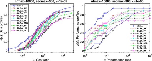
Following the data profile of Mor'e and Wild [59] and the performance profile of Dolan and Mor'e [60],

• the data profile ${\delta }_s\left(\kappa \right)$ of the solver s for a positive value of κ measures the fraction of problems that the solver s can solve with at most $\kappa (n+1)$ function evaluations, where n is the dimension of problems,

• the performance profile ${\rho }_s\left(\tau \right)$ of the solver s for a positive value of τ measures the relative efficiency of the solver s in solving the set of problems.

In particular, the fraction of problems that the solver s wins compared to the other solvers is ${\rho }_s\left(1\right)$ and the fraction of problems for sufficiently large τ (or κ) that the solver s can solve is ${\rho }_s\left(\tau \right)$ (or ${\delta }_s(\kappa$)). The measure for efficiency considered in this paper is the number nf of function evaluations. The efficiency with respect to nf is called nf efficiency. All algorithms terminated when exactly one of the conditions $\Vert F\left(x_{ϵ}\right)\Vert \le {10}^{-5}$, $\mathtt{\text{nf}}\le \mathtt{\text{nfmax}}=10000$, and $\mathtt{\text{sec}}\le \mathtt{\text{secmax}}=360$ sec was satisfied. Here sec denotes time in seconds.

To evaluate their robustness and efficiency, we plot the data and performance profiles of all algorithms. From Figure 1, we conclude that SILSA is competitive with the other algorithms. Of the 112 test functions, SILSA is able to solve 95% of them, while also having the lowest number of function evaluations on 45% of these problems.

Figure 1. Results for problems with $n\in \{10,50,300,500,1000,5000\}$, the maximum number of function reevaluations ($\mathtt{\text{nfmax}}=10000$), the maximum time in seconds ($\mathtt{\text{secmax}}=360$ sec), and $ϵ={10}^{-5}$: Data profiles $\delta \left(\kappa \right)$ (left) in dependence of a bound κ on the cost ratio, performance profiles $\rho \left(\tau \right)$ (right) in dependence of a bound τ on the performance ratio, in terms of nf. Problems solved by no solver are ignored.

6. Conclusion

The paper discusses an improved derivative-free line search method for nonlinear monotone equations. Our line search is a combination of the basic line search algorithm proposed by Solodov and Svaiter [18] and a novel subspace inertial point whose goal is to speed up reaching an approximate solution of nonlinear monotone equations. The subspace is generated based on a finite number of the previous MP points such that a point with largest residual norm among the previous MP points is replaced by a new evaluated point. The global convergence and worst case complexity results are proved. Numerical results show that our improved line search method is competitive with the state-of-the-art derivative-free methods.

7. Test problems in Matlab

The Matlab codes of all 18 test problems are as follows:

The problems 1–4, 6–8, 10, 13 are from [46], the problem 5 is from [14], the problems 9, 14, 15 are from [61], the problems 12 is from [62], and the problems 16-18 are from the present paper. To obtain the problems 16-18, the nonlinear complementarity problem $(x,s)\ge 0,s=F\left(x\right),x^{T}s=0$ is converted to the nonsmooth equations (45) $\left(\begin{array}{c}s-F\left(x\right)\\ min\{x,s\}\end{array}\right)=0,$(45) where F is a monotone operator. Following [63], by defining $\varphi (\mu ,a,b):=a+b-\sqrt{(a-b{)}^2+4\mu }\text{for all}(\mu ,a,b)\in {\mathbb{R}}^3,$the problem (45(45) $\left(\begin{array}{c}s-F\left(x\right)\\ min\{x,s\}\end{array}\right)=0,$(45) ) is transformed into $\left(\begin{array}{c}s-F\left(x\right)\\ \varphi (\mu ,x_1,s_1)\\ \varphi (\mu ,x_2,s_2)\\ \varphi (\mu ,x_n,s_n)\end{array}\right)=0.$For all test problems, the initial points were chosen to be $x_i=i/(i+2)$ for $i=1,\dots ,n$.

Disclosure statement

No potential conflict of interest was reported by the author(s).

Additional information

Funding

The first author acknowledges financial support of the Austrian Science Foundation under Project No. P 34317. The second author is grateful to King Fahd University of Petroleum and Minerals for providing excellent research facilities. The third author is supported by an FWO junior postdoctoral fellowship [12AK924N]. In addition, she received funding from the Flemish Government (AI Research Program). Susan Ghaderi is affiliated with Leuven.AI - KU Leuven Institute for AI, B-3000, Leuven, Belgium.

References

- Chorowski J, Zurada JM. Learning understandable neural networks with nonnegative weight constraints. IEEE Trans Neural Netw Learn Syst. 2015;26(1):62–69. doi: 10.1109/TNNLS.2014.2310059
- Blumensath T. Compressed sensing with nonlinear observations and related nonlinear optimization problems. IEEE Trans Inf Theory. 2013;59:3466–3474. doi: 10.1109/TIT.2013.2245716
- Candes EJ, Li X, Soltanolkotabi M. Phase retrieval via wirtinger flow: theory and algorithms. IEEE Trans Inf Theory. 2015 Apr;61(4):1985–2007. doi: 10.1109/TIT.2015.2399924
- Dirkse SP, Ferris MC. Mcplib: a collection of nonlinear mixed complementarity problems. Optim Methods Softw. 1995 Jan;5(4):319–345. doi: 10.1080/10556789508805619
- Ahookhosh M, Amini K, Bahrami S. Two derivative-free projection approaches for systems of large-scale nonlinear monotone equations. Numer Algorithms. 2012 Oct;64(1):21–42. doi: 10.1007/s11075-012-9653-z
- Ahookhosh M, Artacho FJA, Fleming RMT, et al. Local convergence of the Levenberg–Marquardt method under Hölder metric subregularity. Adv Comput Math. 2019 Jun;45(5-6):2771–2806. doi: 10.1007/s10444-019-09708-7
- Ahookhosh M, Fleming RMT, Vuong PT. Finding zeros of hölder metrically subregular mappings via globally convergent Levenberg–Marquardt methods. Optim Methods Softw. 2020 Jan;37(1):113–149. doi: 10.1080/10556788.2020.1712602
- Amini K, Shiker MA, Kimiaei M. A line search trust-region algorithm with nonmonotone adaptive radius for a system of nonlinear equations. 4OR. 2016;14(2):133–152. doi: 10.1007/s10288-016-0305-3
- Brown PN, Saad Y. Convergence theory of nonlinear Newton–Krylov algorithms. SIAM J Optim. 1994;4(2):297–330. doi: 10.1137/0804017
- Dennis JE, Moré JJ. A characterization of superlinear convergence and its application to quasi-Newton methods. Math Comput. 1974;28(126):549–560. doi: 10.1090/mcom/1974-28-126
- Esmaeili H, Kimiaei M. A trust-region method with improved adaptive radius for systems of nonlinear equations. Math Methods Oper Res. 2016;83(1):109–125. doi: 10.1007/s00186-015-0522-0
- Kimiaei M. Nonmonotone self-adaptive Levenberg–Marquardt approach for solving systems of nonlinear equations. Numer Funct Anal Optim. 2018;39(1):47–66. doi: 10.1080/01630563.2017.1351988
- Kimiaei M, Esmaeili H. A trust-region approach with novel filter adaptive radius for system of nonlinear equations. Numer Algorithms. 2016;73(4):999–1016. doi: 10.1007/s11075-016-0126-7
- Li D, Fukushima M. A globally and superlinearly convergent Gauss–Newton-based bfgs method for symmetric nonlinear equations. SIAM J Numer Anal. 1999;37(1):152–172. doi: 10.1137/S0036142998335704
- Yamashita N, Fukushima M. On the Rate of Convergence of the Levenberg-Marquardt Method. In: Alefeld G, Chen X, editors. Topics in Numerical Analysis. Springer Vienna.2001. p. 239–249.
- Yuan Y. Recent advances in numerical methods for nonlinear equations and nonlinear least squares. NACO. 2011;1(1):15–34. doi: 10.3934/naco.2011.1.15
- Zhou G, Toh KC. Superlinear convergence of a Newton-type algorithm for monotone equations. J Optim Theory Appl. 2005;125(1):205–221. doi: 10.1007/s10957-004-1721-7
- Solodov MV, Svaiter BF. A globally convergent inexact Newton method for systems of monotone equations. In: Reformulation: Nonsmooth, piecewise smooth, semismooth and smoothing methods. Springer; 1998. p. 355–369.
- Al-Baali M, Narushima Y, Yabe H. A family of three-term conjugate gradient methods with sufficient descent property for unconstrained optimization. Comput Optim Appl. 2014 May;60(1):89–110. doi: 10.1007/s10589-014-9662-z
- Aminifard Z, Babaie-Kafaki S. A modified descent Polak–Ribiére–Polyak conjugate gradient method with global convergence property for nonconvex functions. Calcolo. 2019;56(2):1–11. doi: 10.1007/s10092-019-0312-9
- Aminifard Z, Hosseini A, Babaie-Kafaki S. Modified conjugate gradient method for solving sparse recovery problem with nonconvex penalty. Signal Process. 2022;193:108424. doi: 10.1016/j.sigpro.2021.108424
- Andrei N. A simple three-term conjugate gradient algorithm for unconstrained optimization. Comput Appl Math. 2013;241:19–29. doi: 10.1016/j.cam.2012.10.002
- Andrei N. Nonlinear conjugate gradient methods for unconstrained optimization. 1. Cham, Switzerland: Springer Cham; 2020.
- Cheng W. A PRP type method for systems of monotone equations. MCM. 2009;50(1-2):15–20.
- Dai YH, Yuan Y. A nonlinear conjugate gradient method with a strong global convergence property. SIAM J Optim. 1999;10(1):177–182. doi: 10.1137/S1052623497318992
- Fletcher R, Reeves CM. Function minimization by conjugate gradients. Comput J. 1964;7(2):149–154. doi: 10.1093/comjnl/7.2.149
- Hager WW, Zhang H. A new conjugate gradient method with guaranteed descent and an efficient line search. SIAM J Optim. 2005;16(1):170–192. doi: 10.1137/030601880
- Hager WW, Zhang H. A survey of nonlinear conjugate gradient methods. Pacific J Optim. 2006;2(1):35–58.
- Ibrahim A, Kumam P, Abubakar AB, et al. A method with inertial extrapolation step for convex constrained monotone equations. J Inequal Appl. 2021;2021(1):1–25. doi: 10.1186/s13660-021-02719-3
- Ibrahim AH, Kumam P, Abubakar AB, et al. Accelerated derivative-free method for nonlinear monotone equations with an application. Numer Linear Algebra Appl. 2021 Nov;29(3):e2424. doi: 10.1002/nla.v29.3
- Ibrahim AH, Kumam P, Sun M, et al. Projection method with inertial step for nonlinear equations: application to signal recovery. J Ind Manag. 2021;19:30–55.
- Liu Y, Storey C. Efficient generalized conjugate gradient algorithms, part 1: theory. J Optim Theory Appl. 1991;69(1):129–137. doi: 10.1007/BF00940464
- Liu Y, Zhu Z, Zhang B. Two sufficient descent three-term conjugate gradient methods for unconstrained optimization problems with applications in compressive sensing. J Appl Math Comput. 2021;68:1787–1816. doi: 10.1007/s12190-021-01589-8
- Lotfi M, Mohammad Hosseini S. An efficient hybrid conjugate gradient method with sufficient descent property for unconstrained optimization. Optim Methods Softw. 2021;37:1725–1739. doi: 10.1080/10556788.2021.1977808
- Papp Z, Rapajić S. FR type methods for systems of large-scale nonlinear monotone equations. Appl Math Comput. 2015;269:816–823.
- Polak E, Ribiere G. Note sur la convergence de méthodes de directions conjuguées. ESAIM: Mathematical Modelling and Numerical Analysis-Modélisation Mathématique et Analyse Numérique. 1969;3(R1):35–43.
- Polyak BT. The conjugate gradient method in extremal problems. USSR Comput Math Math Phys. 1969;9(4):94–112. doi: 10.1016/0041-5553(69)90035-4
- Zhang L, Zhou W, Li DH. A descent modified Polak–Ribière–Polyak conjugate gradient method and its global convergence. IMA J Numer. 2006;26(4):629–640. doi: 10.1093/imanum/drl016
- Alvarez F. Weak convergence of a relaxed and inertial hybrid projection-proximal point algorithm for maximal monotone operators in hilbert space. SIAM J Optim. 2004 Jan;14(3):773–782. doi: 10.1137/S1052623403427859
- Alvarez F, Attouch H. An inertial proximal method for maximal monotone operators via discretization of a nonlinear oscillator with damping. Set-Valued Var Anal. 2001;9(1):3–11. doi: 10.1023/A:1011253113155
- Attouch H, Peypouquet J, Redont P. A dynamical approach to an inertial forward-backward algorithm for convex minimization. SIAM J Optim. 2014;24(1):232–256. doi: 10.1137/130910294
- Beck A, Teboulle M. A fast iterative shrinkage-thresholding algorithm for linear inverse problems. SIAM J Imaging Sci. 2009;2(1):183–202. doi: 10.1137/080716542
- Boţ RI, Grad SM. Inertial forward–backward methods for solving vector optimization problems. Optimization. 2018 Feb;67(7):959–974. doi: 10.1080/02331934.2018.1440553
- Boţ RI, Nguyen DK. A forward-backward penalty scheme with inertial effects for monotone inclusions, applications to convex bilevel programming. Optimization. 2018 Dec;68(10):1855–1880.
- Boţ R, Sedlmayer M, Vuong PT. A relaxed inertial forward-backward-forward algorithm for solving monotone inclusions with application to GANs. arXiv e-prints, arXiv:2003.07886, 2020 Mar.
- Ibrahim AH, Kimiaei M, Kumam P. A new black box method for monotone nonlinear equations. Optimization. 2021 Nov;72:1119–1137. doi: 10.1080/02331934.2021.2002326
- Kimiaei M, Neumaier A. Efficient global unconstrained black box optimization. Math Program Comput. 2022 Feb;14:365–414. doi: 10.1007/s12532-021-00215-9
- Dai YH, Liao LZ. New conjugacy conditions and related nonlinear conjugate gradient methods. Appl Math Optim. 2001 Jan;43(1):87–101. doi: 10.1007/s002450010019
- Li M. An Liu-Storey-type method for solving large-scale nonlinear monotone equations. Numer Funct Anal Optim. 2014;35(3):310–322. doi: 10.1080/01630563.2013.812656
- Cartis C, Sampaio P, Toint P. Worst-case evaluation complexity of non-monotone gradient-related algorithms for unconstrained optimization. Optimization. 2014 Jan;64(5):1349–1361. doi: 10.1080/02331934.2013.869809
- Curtis FE, Lubberts Z, Robinson DP. Concise complexity analyses for trust region methods. Optim Lett. 2018 Jun;12(8):1713–1724. doi: 10.1007/s11590-018-1286-2
- Dodangeh M, Vicente LN. Worst case complexity of direct search under convexity. Math Program. 2014 Nov;155(1-2):307–332. doi: 10.1007/s10107-014-0847-0
- Dodangeh M, Vicente LN, Zhang Z. On the optimal order of worst case complexity of direct search. Optim Lett. 2015 Jun;10(4):699–708. doi: 10.1007/s11590-015-0908-1
- Vicente L. Worst case complexity of direct search. EURO J Comput Optim. 2013 May;1(1-2):143–153. doi: 10.1007/s13675-012-0003-7
- Ivanov B, Milovanović GV, Stanimirović PS. Accelerated dai-liao projection method for solving systems of monotone nonlinear equations with application to image deblurring. J Glob Optim. 2022 Jul;85(2):377–420. doi: 10.1007/s10898-022-01213-4
- Abubakar AB, Kumam P. A descent Dai-Liao conjugate gradient method for nonlinear equations. Numer Algorithms. 2018 May;81(1):197–210. doi: 10.1007/s11075-018-0541-z
- Huang F, Deng S, Tang J. A derivative-free memoryless BFGS hyperplane projection method for solving large-scale nonlinear monotone equations. Soft Comput. 2022 Oct;27(7):3805–3815. doi: 10.1007/s00500-022-07536-4
- Sabi'u J, Shah A, Stanimirović PS, et al. Modified optimal Perry conjugate gradient method for solving system of monotone equations with applications. Appl Numer Math. 2023 Feb;184:431–445. doi: 10.1016/j.apnum.2022.10.016
- Moré JJ, Wild SM. Benchmarking derivative-free optimization algorithms. SIAM J Optim. 2009 Jan;20(1):172–191. doi: 10.1137/080724083
- Dolan ED, Moré JJ. Benchmarking optimization software with performance profiles. Math Program. 2002 Jan;91(2):201–213. doi: 10.1007/s101070100263
- La Cruz W, Martínez J, Raydan M. Spectral residual method without gradient information for solving large-scale nonlinear systems of equations. Math Comput. 2006;75(255):1429–1448. doi: 10.1090/S0025-5718-06-01840-0
- Gao P, He C. An efficient three-term conjugate gradient method for nonlinear monotone equations with convex constraints. Calcolo. 2018 Nov;55(4):53. doi: 10.1007/s10092-018-0291-2
- Geiger C, Kanzow C. On the resolution of monotone complementarity problems. Comput Optim Appl. 1996 Mar;5(2):155–173. doi: 10.1007/BF00249054