Portfolio reshaping under 1st-order stochastic dominance constraints by the exact penalty function methods

Abstract

The paper studies a financial portfolio selection problem under 1st-order stochastic dominance constraints. These constraints constitute lower bounds on the return profile of the portfolio. In particular, they allow searching for a better portfolio than some reference portfolio by comparing their cumulative distribution functions. Candidate objective functions are the average return, a value at risk, or the average value at risk. The optimization problems obtained are computationally hard because of possibly non-convex constraints and possibly discontinuous objective functions. In the case of a discrete distribution of the return, we develop numerical procedures to solve the problem. The proposed approach uses new exact penalty functions to tackle with the 1st-order stochastic dominance constraints. The resulting penalized objective function is further optimized be the stochastic successive smoothing method as a local optimizer within some branch and bound global optimization scheme. The approach is numerically and graphically illustrated on small portfolio selection problems up to dimension 10.

Keywords:

• Global optimization
• exact penalty method
• stochastic dominance

1. Introduction

We consider the general, constrained optimization problem (1) $\begin{array}{r}\mathrm{minimize}f\left(x\right),x\in \mathcal{X},\end{array}$(1) where the set $\mathcal{X}\subset {\mathbb{R}}^n$ constitutes the set of feasible solutions. The projective exact penalty method (cf. [1]) involves a map ${\pi }_{\mathcal{X}}:{\mathbb{R}}^n\to \mathcal{X}$ such that (2) $\begin{array}{rl}{\pi }_{\mathcal{X}}\left({\mathbb{R}}^n\right)& \subset \mathcal{X}\mathrm{and}\\ {\pi }_{\mathcal{X}}\left(x\right)& =x\text{for every}x\in \mathcal{X}.\end{array}$(2) The map ${\pi }_{\mathcal{X}}$ in (2(2) $\begin{array}{rl}{\pi }_{\mathcal{X}}\left({\mathbb{R}}^n\right)& \subset \mathcal{X}\mathrm{and}\\ {\pi }_{\mathcal{X}}\left(x\right)& =x\text{for every}x\in \mathcal{X}.\end{array}$(2) ) is not specified. For $\mathcal{X}$ convex, the projection (3) $\begin{array}{r}{\pi }_{\mathcal{X}}\left(x\right)=\arg \min \{\Vert y-x\Vert :y\in \mathcal{X}\}\end{array}$(3) is well-defined and thus is a candidate for the global optimization problem (4(4) $\begin{array}{r}\mathrm{minimize}f\left({\pi }_{\mathcal{X}}\right(x\left)\right)+\Vert x-{\pi }_{\mathcal{X}}\left(x\right)\Vert ,x\in {\mathbb{R}}^n,\end{array}$(4) ). However, the projection (3(3) $\begin{array}{r}{\pi }_{\mathcal{X}}\left(x\right)=\arg \min \{\Vert y-x\Vert :y\in \mathcal{X}\}\end{array}$(3) ) might not be available at cheap computational costs. 

For a star domain $\mathcal{X}$, there exists a point $x^0\in \mathcal{X}$ so that every line segment $[x,x^0]\{\lambda x^0+(1-\lambda )x:\lambda \in [0,1\left]\right\}$ is fully contained in $\mathcal{X}$, provided that $x\in \mathcal{X}$. The function $\begin{array}{r}{\pi }_{\mathcal{X}}\left(x\right)={\lambda }_x{x}^0+(1-{\lambda }_x)x,x\in \mathcal{X},\end{array}$where $\begin{array}{r}{\lambda }_x:=sup\{\lambda :\lambda x^0+(1-\lambda )x\in \mathcal{X}\},\end{array}$as well satisfies the conditions (2(2) $\begin{array}{rl}{\pi }_{\mathcal{X}}\left({\mathbb{R}}^n\right)& \subset \mathcal{X}\mathrm{and}\\ {\pi }_{\mathcal{X}}\left(x\right)& =x\text{for every}x\in \mathcal{X}.\end{array}$(2) ).

For a single-valued and continuous projection mapping ${\pi }_{\mathcal{X}}(\cdot )$, the global and local solutions of the constrained problem (1(1) $\begin{array}{r}\mathrm{minimize}f\left(x\right),x\in \mathcal{X},\end{array}$(1) ) and the unconstrained, global optimization problem (4) $\begin{array}{r}\mathrm{minimize}f\left({\pi }_{\mathcal{X}}\right(x\left)\right)+\Vert x-{\pi }_{\mathcal{X}}\left(x\right)\Vert ,x\in {\mathbb{R}}^n,\end{array}$(4) coincide. Hence, the global, unconstrained optimization problem (4(4) $\begin{array}{r}\mathrm{minimize}f\left({\pi }_{\mathcal{X}}\right(x\left)\right)+\Vert x-{\pi }_{\mathcal{X}}\left(x\right)\Vert ,x\in {\mathbb{R}}^n,\end{array}$(4) ) can be considered instead of the constrained optimization problem (1(1) $\begin{array}{r}\mathrm{minimize}f\left(x\right),x\in \mathcal{X},\end{array}$(1) ).

The problem (4(4) $\begin{array}{r}\mathrm{minimize}f\left({\pi }_{\mathcal{X}}\right(x\left)\right)+\Vert x-{\pi }_{\mathcal{X}}\left(x\right)\Vert ,x\in {\mathbb{R}}^n,\end{array}$(4) ) is not necessarily smooth nor convex. So solving (4(4) $\begin{array}{r}\mathrm{minimize}f\left({\pi }_{\mathcal{X}}\right(x\left)\right)+\Vert x-{\pi }_{\mathcal{X}}\left(x\right)\Vert ,x\in {\mathbb{R}}^n,\end{array}$(4) ) requires applying non-smooth local and global optimization methods (cf. [1]).

The present paper outlines the described methodology for a financial portfolio optimization problem under specific constraints, namely 1st-order stochastic dominance constraints (FSD), where each feasible portfolio stochastically dominates a given reference portfolio. This means that a decision maker with non-decreasing utility function will prefer any feasible portfolio to the reference one. Such portfolio optimization settings were considered in [2,3] (with the 2nd-order stochastic dominance constraints, SSD) and in [4] (for linear problems with 1st-order stochastic dominance constraints). Problems with FSD constraints are much harder than the ones with SSD constraints, because the former are non-convex. Noyan and Ruszczyński [5] reduce such problems to linear mixed-integer problems. The present paper develops a different approach to such problems, which is applicable to the nonlinear case as well. Our approach consists in an application of the exact penalty method to remove the FSD constraints and solution of the obtained penalty problem by non-smooth global optimization methods.

Outline of the paper.

First, Section 2 reviews the literature on decision-making and portfolio optimization under stochastic dominance constraints.

In Section 3, we set the problem of a portfolio optimization under 1st-order stochastic dominance constraints and provide some examples of such problems. Next (cf. Section 4), we reduce the portfolio optimization problem under 1st-order stochastic dominance constraints to the unconstrained problems by means of new exact projective non-smooth and discontinuous penalty functions.

Forth, we review the successive smoothing method for local optimization of non-smooth and discontinuous functions. This method is used as a local optimizer within the branch and bound framework for the global optimization of the penalty functions. We finally give numerical illustrations (Section 5) of the proposed approach to financial portfolio optimization under 1st-order stochastic dominance constraints on portfolios containing up to 10 components with one risk-free asset.

2. Literature review

The problem of financial portfolio optimization belongs to the class of decision-making problems under uncertainty. The choice of a particular portfolio is accompanied by an uncertain result in the form of a distribution of future returns. This and more general decision problems under stochastic uncertainty are studied in the theory of stochastic programming (cf. [6]). In the general case, the formalization of such problems is carried out using preferences defined on the set of possible uncertain results of decisions made. Preferences establish partial order relationships on the set of decision outcomes, i.e. they satisfy the axioms of reflexivity, transitivity, and antisymmetry. Partial order relations make it possible to narrow the choice of preferable solutions to a subset of non-dominated alternatives. Under additional assumptions about the properties of preferences, the latter can be represented in a numerical form, and then the problem of choosing preferred outcomes turns into a problem of multi-objective optimization. A discussion of stochastic programming problems from this perspective can be found in [7]. Conversely, any numerical function on the set of outcomes specifies a preference relation.

In optimization and financial portfolio management problems, investments are often allocated according subject to utility and risk criteria. The original settings of this type were proposed by Markowitz [8] and Roy [9], who used the mean return as a measure of utility and the variance of returns as a measure of risk. An attractive feature of these formulations is the relative simplicity of the resulting optimization problems.

Subsequently, other utility and risk measures were proposed and used, such as quantiles, averaged quantiles, semi-deviations of returns from the average value, probabilities of returns falling into a profit or loss area, general coherent risk measures, and others (the references include [10–25], cf. also the references therein). The corresponding decision selection problems are computationally more complex and require adapting known methods, or even developing new solution methods. For example in [26], the problems of optimizing a financial portfolio in terms of averaged quantiles are reduced to a linear programming problem and can be effectively solved by existing software tools. However, problems that involve quantiles or probabilities are much more difficult because they are non-convex and non-smooth with a possibly non-convex and disconnected admissible region. The problem may be even harder, if the return depends nonlinearly on the portfolio structure (see, e.g. the discussion of the properties of these problems in [12,13]). For example, in the works by Noyan et al. [4], Benati and Rizzi [11], Luedtke et al. [18], Norkin and Boyko [19], Kibzun et al. [16] and Norkin et al. [20], such problems are reduced to problems of mixed-integer programming in the case of a discrete distribution of random data. Gaivoronski and Pflug [13] developed a special method for smoothing a variational series to optimize a portfolio by a quantile criterion. Wozabal et al. [25] give a review of the quantile constrained portfolio selection problem, present a difference-of-convex representation of involved quantiles, and develop a branch and bound algorithm to solve the reformulated problem.

On the other hand, natural relations of stochastic dominance of the first, second and higher orders are known on the set of probability distributions. For example, the first order stochastic dominance relation is defined as the excess of one distribution function over another distribution function. The relation of stochastic dominance of the second order is determined by the relation of the integrals of the distribution functions of random variables. With the second-order stochastic dominance relation, the decision maker's negative attitude towards risk can be expressed (see a discussion of these issues in [27,28]).

A natural question arises about the connection between decision-making problems in a multi-criteria formulation and in terms of certain preference relations, in particular, stochastic dominance relations. The connection between mean-risk models and second-order stochastic dominance relations was studied in the works by Ogryczak and Ruszczyński [29–31]. In the works by Dentcheva and Ruszczyński [27,32] it is shown under what conditions the problem of decision-making in terms of preference relations is reduced to the problem of optimizing a numerical indicator.

Dentcheva and Ruszczyński [2,3] proposed a mixed financial portfolio optimization model in which a numerical criterion is optimized, and constraints are specified using second-order stochastic dominance relations. The feasible set in this setting consists of decisions, which dominate some reference one and are preferred by any risk averse decision maker. In the case of a discrete distribution of random data, the problem is reduced to a linear programming problem of (large) dimension. These works have given rise to a large stream of work on stochastic optimization problems under second-order stochastic dominance constraints (see the reviews by Gutjahr and Pichler [7], Dai et al. [33], Dentcheva and Ruszczyński [34] and Fábián et al. [35]).

Noyan et al. [4,5] and Dentcheva and Ruszczyński [36] considered similar mixed problems, but with first-order stochastic dominance relations in the constraints. To solve them, a method of reduction to problems of linear mixed-integer programming with subsequent continuous relaxation of Boolean constraints and the introduction of additional cutting constraints is proposed. The paper [33] develops a quite different approach to solving the problem based on the dual reformulation from [37] by discretization of the space of one-dimensional utilities by step-wise functions, smoothing the latter, and applying the stochastic gradient method for the (local) optimization of the approximate dual function. Dentcheva et al. [38] studied the stability of these problems with respect to perturbation of the involved distributions on the basis of general studies of the stability of stochastic programming problems.

In this article, we consider similar financial portfolio optimization problems under 1st-order stochastic dominance constraints, but from a different point of view and apply a different solution approach that is also applicable to problems with nonlinear random return functions. This problem is viewed as the problem of optimizing the risk profile of the portfolio according to the preferences of the decision maker. Namely, the decision maker sets the desired risk profile (the form of the cumulative distribution function) and tries to find an acceptable portfolio that dominates this risk profile. This is one statement, and the other is that, under the condition of the existence of an admissible portfolio, i.e. portfolio dominating some reference portfolio, it can be any index or risk-free portfolio, choose a portfolio with the desired risk profile by optimizing one or another function (for example risk measures, as average quantiles, etc.).

In this way it is possible to satisfy the needs of both a risk seeking decision maker and a risk averse decision maker. In the first case, the average quantile function for high returns is maximized, and in the second case, the mean quantile function for low returns is maximized, in both cases with a lower bound on the quantile risk profile. In the first case, the risk profile is stretched, and in the second case, it is compressed and becomes more like a profile of a deterministic value. The reshaping of the risk profile can be made both through selection of different objective function and by adding new securities to the portfolio, e.g. as commodities, etc., cf. [39].

In the problems under consideration, the objective function is nonlinear, non-convex, and possibly non-smooth or even discontinuous, and the number of constraints is continual (uncountable). But when the reference profile has a stepped character, one can limit oneself to a finite number of restrictions by the number of steps of the reference profile. In this problem, the admissible area may turn out to be non-convex and disconnected. Thus, the problem under consideration is a global optimization problem with highly complex and nonlinear constraints. To solve it, we first reduce it to an unconstrained global optimization problem by applying new penalty functions, namely, discontinuous penalty functions as in [40,41] and the so-called projective penalty functions as in [1,42]. In the first case, the objective function outside the allowable area is extended by large but finite penalty values, and in the second case, it is extended at infeasible points by summing the value of the objective function in the projection of this point onto the feasible set and the distance to this projection. In this case, the projection is made in the direction of some known internal feasible point. After such a transformation, the problem is still a complex unconstrained global optimization problem. In order to solve it, we further apply the method of successive smoothing of this penalty function, i.e. we minimize successive smoothed approximations of the penalized function, starting from relatively large smoothing parameters with its gradual decreasing to zero. It is known that the smoothed functions can be optimized by the method of stochastic gradients, where the latter have the form of finite difference vectors in random directions, cf. [43–46]. Here, smoothing plays a dual role. Firstly, it allows optimizing non-smooth and discontinuous functions and, secondly, it levels out shallow local extrema. Although smoothing makes it possible to ignore small local extrema, it does not guarantee convergence to the global extrema. Therefore, we put the method of sequential smoothing in a general scheme of the stochastic branch and bound method, where the smoothing method plays the role of a local optimizer on subsets of the optimization area. The scheme of the branch and bound method is designed in such a way that the calculations are concentrated in the most promising areas of the search for the global extrema. Our approach is similar to that of Dai et al. [33], but applied to the primal problem, it applies an exact penalty method instead of the Lagrangian one, and optimizes the penalized function by stochastic finite-difference gradient methods. Besides, we provide global search by a specific stochastic branch and bound algorithm, which is well-suited for parallelization.

This article describes the financial portfolio optimization model with 1st-order stochastic dominance constraints and illustrates the proposed approach to its solution on the problems of reshaping the risk profile of portfolios of small dimension. At the same time, the results of changing the shape of the risk profile are presented in graphical form, which allows visually comparing the resulting profile with the reference one, and, if necessary, continue adaptation of the profile to the preferences of the decision maker.

3. Mathematical problem setting

The financial portfolio is described by a vector $x=(x_1,\dots ,x_n{)}^{\prime }$ of values $x_i$ and by a random vector of returns $\omega =({\omega }_1,\dots ,{\omega }_n{)}^{\prime }\in \mathrm{\Omega }$ of assets, $i=1,\dots ,n$, in some fixed time interval; $(\cdot {)}^{\prime }$ denotes the transposition of a vector. Denote by $\begin{array}{r}X\{x\in {\mathbb{R}}^n:\sum _{i=1}^n{x}_i\le 1,x_i\ge c_i\ge -\mathrm{\infty }\}\end{array}$the set of admissible portfolios with a unit maximal total cost of the whole portfolio, $c_i$ is a lower bound on the value of component i of the portfolio (e.g. a short-selling constraint or a limitation on borrowing assets). In the definition of the set X, the inequality ${\sum }_{i=1}^n{x}_i\le 1$ is used, which means that $x_{0}1-{\sum }_{i=1}^n{x}_i$ – the non-invested funds – have zero yield. The portfolio is characterized by a random return $f(x,\omega )={\omega }^{\prime }x$, by the mean return $\mu \left(x\right)={\mathbb{E}}_{\omega }f(x,\omega )=\sum _{i=1}^n{x}_i{\mathbb{E}}_{\omega }{\omega }_i$ for the considered period of time and by the variance of return ${\sigma }^2\left(x\right)={\mathbb{E}}_{\omega }\left(f\right(x,\omega )-{\mathbb{E}}_{\omega }f(x,\omega ){)}^2$, where ${\mathbb{E}}_{\omega }$ denotes the mathematical expectation with respect to the distribution of random variable ω.

The classical financial portfolio models assume a linear dependence of the return on the portfolio structure, for which alternative problem reformulations are available. Nonlinearities appear when random returns are modelled by some parametric distribution. Another example of nonlinear portfolio return appears in the dynamic portfolio optimization problem with fixed mix portfolio control strategy, cf. [47].

Suppose the random vector ω is given by a discrete (an empirical, e.g.) distribution $\{{\omega }^1,\dots ,{\omega }^m\}$ with equiprobable values ${\omega }^i\in {\mathbb{R}}^n$, $i=1,2,\dots ,m$. Then the average portfolio return $\mu \left(x\right)=\mathbb{E}{\omega }^{\prime }x$ and the cumulative distribution function (CDF) of the portfolio return ${\mathcal{F}}_x\left(t\right)=\mathrm{Pr}\{{\omega }^{\prime }x\le t\}$ are given by $\begin{array}{r}f\left(x\right)={\mu }_m\left(x\right)=\frac{1}{m}\sum _{i=1}^m({\omega }^i{)}^{\prime }x\end{array}$and $\begin{array}{r}{\mathcal{F}}_x\left(t\right)={\mathcal{F}}_{x,m}\left(t\right)=m^{-1}\mathrm{\#}\{i:({\omega }^i{)}^{\prime }x\le t\}.\end{array}$The portfolio optimization problem under 1st-order stochastic dominance constraint is (5) $\begin{array}{rl}\mathrm{maximize}& f\left(x\right)\end{array}$(5) (6) $\begin{array}{rl}\text{subject to}& {\mathcal{F}}_x\left(t\right)\le {\mathcal{F}}_{\mathit{ref}}\left(t\right)\text{for all}t\in \mathbb{R}\mathrm{and}x\in X.\end{array}$(6) The objective function $f\left(x\right)$ in (5(5) $\begin{array}{rl}\mathrm{maximize}& f\left(x\right)\end{array}$(5) ) quantifies the profit, which is to be maximized. As objectives $f\left(x\right)$ in the master problem (5(5) $\begin{array}{rl}\mathrm{maximize}& f\left(x\right)\end{array}$(5) ), we consider

• the mean value $\mu \left(x\right)$,

• some Value-at-Risk function (${\mathrm{V}@\mathrm{R}}_{\gamma }\left(x\right)$) at risk level $\gamma \in (0,1)$,

• the average Value-at-Risk function $\begin{array}{r}{\mathrm{AV}@\mathrm{R}}_{\alpha ,\text{β}}\left(x\right)\frac{1}{\text{β}-\alpha }{\int }_{\alpha }^{\text{β}}{\mathrm{V}@\mathrm{R}}_{\gamma }\left(x\right)\mathrm{d}\gamma ,0\le \alpha <\text{β}\le 1,\end{array}$in particular ${\mathrm{AV}@\mathrm{R}}_{\gamma }\left(x\right){\mathrm{AV}@\mathrm{R}}_{\gamma ,1}\left(x\right)$ and ${\mathrm{AV}@\mathrm{R}}_{0,1}\left(x\right)=\mu \left(x\right)$.

The constraints (6(6) $\begin{array}{rl}\text{subject to}& {\mathcal{F}}_x\left(t\right)\le {\mathcal{F}}_{\mathit{ref}}\left(t\right)\text{for all}t\in \mathbb{R}\mathrm{and}x\in X.\end{array}$(6) ) address risk: the cumulative distribution function ${\mathcal{F}}_x(\cdot )$ of the feasible portfolio x must not be worse than the reference function ${\mathcal{F}}_{\mathit{ref}}\left(t\right)$ (also called a reference risk profile) for all $t\in \mathbb{R}$. The reference function itself may be given by ${\mathcal{F}}_{x_{\mathit{ref}}}(t+\delta (t\left)\right)$, where $x_{\mathit{ref}}$ is some reference portfolio with cumulative distribution function ${\mathcal{F}}_{x_{\mathit{ref}}}\left(t\right))=Pr\{{\omega }^{\prime }{x}_{\mathit{ref}}\le t\}$.

We formally can associate some random variable ${\xi }_{\mathit{ref}}$ with the CDF ${\mathcal{F}}_{\mathit{ref}}\left(t\right)$. Then, the family of inequalities (6(6) $\begin{array}{rl}\text{subject to}& {\mathcal{F}}_x\left(t\right)\le {\mathcal{F}}_{\mathit{ref}}\left(t\right)\text{for all}t\in \mathbb{R}\mathrm{and}x\in X.\end{array}$(6) ) ensures that the random variable ${\xi }_x={\omega }^{\prime }x$ dominates the random variable ${\xi }_{\mathit{ref}}$ in 1st stochastic order. We further remark that there can be several stochastic dominance constraints with corresponding reference CDF ${\mathcal{F}}_{\mathit{ref}}^i$, which can be replaced by the single CDF ${\mathcal{F}}_{\mathit{ref}}=\underset{i}{min}{\mathcal{F}}_{\mathit{ref}}^i$.

The constraints (6(6) $\begin{array}{rl}\text{subject to}& {\mathcal{F}}_x\left(t\right)\le {\mathcal{F}}_{\mathit{ref}}\left(t\right)\text{for all}t\in \mathbb{R}\mathrm{and}x\in X.\end{array}$(6) ) are tight– often too tight to ensure a non-empty set of feasible solutions. The function $\delta \left(t\right)\ge 0$ relaxes these tight constraints by accepting higher losses at given probabilities.

The function ${\mathcal{F}}_x(\cdot )$ is non-decreasing and continuous from the right (upper semicontinuous), the functions ${\mathcal{F}}_{\mathit{ref}}(\cdot )$ and $\delta (\cdot )$ are assumed right continuous.

Lemma 3.1

The feasible set in (6(6) $\begin{array}{rl}\text{subject to}& {\mathcal{F}}_x\left(t\right)\le {\mathcal{F}}_{\mathit{ref}}\left(t\right)\text{for all}t\in \mathbb{R}\mathrm{and}x\in X.\end{array}$(6) ) is either empty or compact.

Proof.

Indeed, define $\begin{array}{rl}{X}^{<}& \{x\in X:{\mathcal{F}}_x^{<}(t)\le {\mathcal{F}}_{\mathit{\text{ref}}}(t)\mathrm{\forall }t\in \mathbb{R}\}\mathrm{and}\\ X^{\le }& \{x\in X:{\mathcal{F}}_x(t)\le {\mathcal{F}}_{\mathit{\text{ref}}}(t)\mathrm{\forall }t\in \mathbb{R}\}\end{array}$with right continuous ${\mathcal{F}}_{\mathit{\text{ref}}}(\cdot )$, ${\mathcal{F}}_x(\cdot )$, and left continuous ${\mathcal{F}}_x^{<}(\cdot )$. On one hand it holds that $X^{\le }\subseteq X^{<}$, since ${\mathcal{F}}_x^{<}\left(t\right)\le {\mathcal{F}}_x\left(t\right)$. On the other hand, if $x\in X^{<}$, then it holds for any t that $\begin{array}{r}{\mathcal{F}}_x\left(t\right)\le \underset{t\leftarrow \tau }{lim}{\mathcal{F}}_x^{<}\left(\tau \right)\le \underset{t\leftarrow \tau }{lim}{\mathcal{F}}_{\mathit{ref}}\left(\tau \right)={\mathcal{F}}_{\mathit{ref}}\left(t\right).\end{array}$So $X^{<}\subseteq X^{\le }$ and, hence, $X^{<}=X^{\le }$. In such case, the function ${\mathcal{F}}_x^{<}\left(t\right)$ appears to be lower semicontinuous in $(x,t)$, hence the sets $\{x\in {\mathbb{R}}^n:{\mathcal{F}}_x^{<}(t)\le {\mathcal{F}}_{\mathit{ref}}(t\left)\right\}$ are closed and the sets $\{x\in X:{\mathcal{F}}_x^{<}(t)\le {\mathcal{F}}_{\mathit{ref}}(t\left)\right\}$ are closed for each t. If the feasible set $X^{\le }=X^{<}$ in (6(6) $\begin{array}{rl}\text{subject to}& {\mathcal{F}}_x\left(t\right)\le {\mathcal{F}}_{\mathit{ref}}\left(t\right)\text{for all}t\in \mathbb{R}\mathrm{and}x\in X.\end{array}$(6) ) is non-empty, then it is closed and bounded and, hence, compact. This completes the proof.

Lemma 3.2

If the function ${\mathcal{F}}_x\left(t\right)$ has only finitely many jumps, e.g. at ${\mathcal{T}}_x=\{{{\omega }^1}^{\prime }x,\dots ,{{\omega }^m}^{\prime }x\},$ then $\begin{array}{r}\{x\in X:{\mathcal{F}}_x(t)\le {\mathcal{F}}_{\mathit{ref}}(t)\mathrm{\forall }t\in \mathbb{R}\}=\{x\in X:{\mathcal{F}}_x(t)\le {\mathcal{F}}_{\mathit{ref}}(t),t\in {\mathcal{T}}_x\}.\end{array}$

Proof.

Let ${\mathcal{T}}_x=\{t_1,t_2,\dots \}$, ${\mathcal{F}}_x\left(t\right)={\mathcal{F}}_x\left(t_k\right)$ for $t\in [t_k,t_{k+1})$, $k\ge 1$, and ${\mathcal{F}}_x\left(t\right)=0$ for $t<t_1$. Then ${\mathcal{F}}_x\left(t\right)={\mathcal{F}}_x\left(t_k\right)\le {\mathcal{F}}_{\mathit{ref}}\left(t_k\right)\le {\mathcal{F}}_{\mathit{ref}}\left(t\right)$ for all $t\in [t_k,t_{k+1})$, $k\ge 1$. Besides, ${\mathcal{F}}_x\left(t\right)=0\le {\mathcal{F}}_{\mathit{ref}}\left(t\right)$ for all $t<t_1$.

An alternative problem formulation. A reformulation of the problem (5(5) $\begin{array}{rl}\mathrm{maximize}& f\left(x\right)\end{array}$(5) )–(6(6) $\begin{array}{rl}\text{subject to}& {\mathcal{F}}_x\left(t\right)\le {\mathcal{F}}_{\mathit{ref}}\left(t\right)\text{for all}t\in \mathbb{R}\mathrm{and}x\in X.\end{array}$(6) ) involves the inverse cumulative distribution functions instead of the CDFs. To this end let $\begin{array}{r}{\mathcal{Q}}_x\left(\alpha \right)\underset{t\in \mathbb{R}}{sup}\{t:{\mathcal{F}}_x(t)\le \alpha \},\alpha \in [0,1],\end{array}$be the return quantile (generalized inverse) function associated with the decision x, and ${\mathcal{Q}}_{\mathit{ref}}\left(\alpha \right)$ be some reference quantile function, continuous from below (lower semicontinuous).

Consider the problem (7) $\begin{array}{rl}\mathrm{maximize}& f\left(x\right)\end{array}$(7) (8) $\begin{array}{rl}\text{subject to}& {\mathcal{Q}}_{\mathit{ref}}\left(\alpha \right)\le {\mathcal{Q}}_x\left(\alpha \right)\text{for all}\alpha \in [0,1]\mathrm{and}x\in X.\end{array}$(8) The following lemmas demonstrate that problem (7(7) $\begin{array}{rl}\mathrm{maximize}& f\left(x\right)\end{array}$(7) )–(8(8) $\begin{array}{rl}\text{subject to}& {\mathcal{Q}}_{\mathit{ref}}\left(\alpha \right)\le {\mathcal{Q}}_x\left(\alpha \right)\text{for all}\alpha \in [0,1]\mathrm{and}x\in X.\end{array}$(8) ) is well-defined and equivalent to the initial problem statement (5(5) $\begin{array}{rl}\mathrm{maximize}& f\left(x\right)\end{array}$(5) )–(6(6) $\begin{array}{rl}\text{subject to}& {\mathcal{F}}_x\left(t\right)\le {\mathcal{F}}_{\mathit{ref}}\left(t\right)\text{for all}t\in \mathbb{R}\mathrm{and}x\in X.\end{array}$(6) ).

Lemma 3.3

Define ${\mathcal{F}}_x^{<}\left(t\right)P\{{\omega }^{\prime }x<t\}$ and ${\mathcal{Q}}_x^{<}\left(\alpha \right)sup\{t:{\mathcal{F}}_x^{<}(t)\le \alpha \}$, then ${\mathcal{Q}}_x\left(\alpha \right)={\mathcal{Q}}_x^{<}\left(\alpha \right),$ both functions ${\mathcal{Q}}_x\left(\alpha \right)$ and ${\mathcal{Q}}_x^{<}\left(\alpha \right)$ are upper semicontinuous in $(x,\alpha )$, and hence the feasible set in (8(8) $\begin{array}{rl}\text{subject to}& {\mathcal{Q}}_{\mathit{ref}}\left(\alpha \right)\le {\mathcal{Q}}_x\left(\alpha \right)\text{for all}\alpha \in [0,1]\mathrm{and}x\in X.\end{array}$(8) ) is compact.

Proof.

First, it holds for any $\alpha \in [0,1]$ that $\begin{array}{r}{\mathcal{Q}}_x^{<}\left(\alpha \right)=sup\{t:{\mathcal{F}}_x^{<}(t)\le \alpha \}\ge sup\{t:{\mathcal{F}}_x(t)\le \alpha \}={\mathcal{Q}}_x\left(\alpha \right).\end{array}$Let us prove the opposite inequality, ${\mathcal{Q}}_x\left(\alpha \right)\ge {\mathcal{Q}}_x^{<}\left(\alpha \right).$ For a given α there exists $t_{\alpha }$ such that ${\mathcal{Q}}_x^{<}\left(\alpha \right)=sup\{t:{\mathcal{F}}_x^{<}(t)\le \alpha \}=t_{x,\alpha }$ and thus ${\mathcal{F}}_x^{<}\left(t\right)\le \alpha$ for all $t\le t_{x,\alpha }$. For any $t<t_{x,\alpha }$, it holds that ${\mathcal{F}}_x\left(t\right)\le {\mathcal{F}}_x^{<}\left(t_{x,\alpha }\right)\le \alpha .$ Hence, we obtain the required opposite inequality, ${\mathcal{Q}}_x\left(\alpha \right)=sup\{t:{\mathcal{F}}_x(t)\le \alpha \}\ge t_{x,\alpha }={\mathcal{Q}}_x^{<}\left(\alpha \right)$ and thus ${\mathcal{Q}}_x\left(\alpha \right)={\mathcal{Q}}_x^{<}\left(\alpha \right).$ Next, the ${\mathcal{Q}}_x^{<}(\cdot )$ is the maximum function, by Aubin and Ekeland [48, Ch. 1, Sec. 1, Prop. 21] it is upper semicontinuous in $(x,\alpha )$. Hence, the feasible set in (8(8) $\begin{array}{rl}\text{subject to}& {\mathcal{Q}}_{\mathit{ref}}\left(\alpha \right)\le {\mathcal{Q}}_x\left(\alpha \right)\text{for all}\alpha \in [0,1]\mathrm{and}x\in X.\end{array}$(8) ) is either empty or compact as intersection of compact sets $\{x\in X:{\mathcal{Q}}_x(\alpha )\ge {\mathcal{Q}}_{\mathrm{ref}}(\alpha \left)\right\}$, $\alpha \in [0,1]$. The proof is complete.

The next lemma states that problems (5(5) $\begin{array}{rl}\mathrm{maximize}& f\left(x\right)\end{array}$(5) )–(6(6) $\begin{array}{rl}\text{subject to}& {\mathcal{F}}_x\left(t\right)\le {\mathcal{F}}_{\mathit{ref}}\left(t\right)\text{for all}t\in \mathbb{R}\mathrm{and}x\in X.\end{array}$(6) ) and (7(7) $\begin{array}{rl}\mathrm{maximize}& f\left(x\right)\end{array}$(7) )–(8(8) $\begin{array}{rl}\text{subject to}& {\mathcal{Q}}_{\mathit{ref}}\left(\alpha \right)\le {\mathcal{Q}}_x\left(\alpha \right)\text{for all}\alpha \in [0,1]\mathrm{and}x\in X.\end{array}$(8) ) are equivalent.

Lemma 3.4

Let ${\mathcal{Q}}_{\mathit{ref}}\left(\alpha \right)sup\{t:{\mathcal{F}}_{\mathit{ref}}(t)\le \alpha \}$ $($cf. (8(8) $\begin{array}{rl}\text{subject to}& {\mathcal{Q}}_{\mathit{ref}}\left(\alpha \right)\le {\mathcal{Q}}_x\left(\alpha \right)\text{for all}\alpha \in [0,1]\mathrm{and}x\in X.\end{array}$(8) )$)$ , where ${\mathcal{F}}_{\mathit{ref}}\left(t\right)$ is the same (right continuous) reference distribution function as in (6(6) $\begin{array}{rl}\text{subject to}& {\mathcal{F}}_x\left(t\right)\le {\mathcal{F}}_{\mathit{ref}}\left(t\right)\text{for all}t\in \mathbb{R}\mathrm{and}x\in X.\end{array}$(6) ). Then the problems (5(5) $\begin{array}{rl}\mathrm{maximize}& f\left(x\right)\end{array}$(5) )–(6(6) $\begin{array}{rl}\text{subject to}& {\mathcal{F}}_x\left(t\right)\le {\mathcal{F}}_{\mathit{ref}}\left(t\right)\text{for all}t\in \mathbb{R}\mathrm{and}x\in X.\end{array}$(6) ) and (7(7) $\begin{array}{rl}\mathrm{maximize}& f\left(x\right)\end{array}$(7) )–(8(8) $\begin{array}{rl}\text{subject to}& {\mathcal{Q}}_{\mathit{ref}}\left(\alpha \right)\le {\mathcal{Q}}_x\left(\alpha \right)\text{for all}\alpha \in [0,1]\mathrm{and}x\in X.\end{array}$(8) ) are equivalent, i.e. they have the same objective function and their feasible sets coincide.

Proof.

We have to prove that (6(6) $\begin{array}{rl}\text{subject to}& {\mathcal{F}}_x\left(t\right)\le {\mathcal{F}}_{\mathit{ref}}\left(t\right)\text{for all}t\in \mathbb{R}\mathrm{and}x\in X.\end{array}$(6) ) and (8(8) $\begin{array}{rl}\text{subject to}& {\mathcal{Q}}_{\mathit{ref}}\left(\alpha \right)\le {\mathcal{Q}}_x\left(\alpha \right)\text{for all}\alpha \in [0,1]\mathrm{and}x\in X.\end{array}$(8) ) define the same feasible set. Assume (6(6) $\begin{array}{rl}\text{subject to}& {\mathcal{F}}_x\left(t\right)\le {\mathcal{F}}_{\mathit{ref}}\left(t\right)\text{for all}t\in \mathbb{R}\mathrm{and}x\in X.\end{array}$(6) ) is fulfilled but (8(8) $\begin{array}{rl}\text{subject to}& {\mathcal{Q}}_{\mathit{ref}}\left(\alpha \right)\le {\mathcal{Q}}_x\left(\alpha \right)\text{for all}\alpha \in [0,1]\mathrm{and}x\in X.\end{array}$(8) ) is not. Then there exists ${\alpha }_0$ such that ${\mathcal{Q}}_{\mathit{ref}}\left({\alpha }_0\right)>{\mathcal{Q}}_x\left({\alpha }_0\right)$. This implies that ${\mathcal{F}}_x\left(Q_{\mathit{ref}}\right({\alpha }_0\left)\right)>{\alpha }_0.$ From here, by assumption (6(6) $\begin{array}{rl}\text{subject to}& {\mathcal{F}}_x\left(t\right)\le {\mathcal{F}}_{\mathit{ref}}\left(t\right)\text{for all}t\in \mathbb{R}\mathrm{and}x\in X.\end{array}$(6) ), ${\mathcal{F}}_{\mathrm{ref}}\left(Q_{\mathit{ref}}\right({\alpha }_0\left)\right)\ge {\mathcal{F}}_x\left(Q_{\mathit{ref}}\right({\alpha }_0\left)\right)>{\alpha }_0$. The supremum in $sup\{t:{\mathcal{F}}_{\mathrm{ref}}(t)\le {\alpha }_0\}$ is achieved at $t={\mathcal{Q}}_{\mathrm{ref}}\left(\alpha \right)$ then ${\mathcal{F}}_{\mathrm{ref}}\left({\mathcal{Q}}_{\mathrm{ref}}\right(\alpha \left)\right)\le {\alpha }_0,$ a contradiction.

Assume (8(8) $\begin{array}{rl}\text{subject to}& {\mathcal{Q}}_{\mathit{ref}}\left(\alpha \right)\le {\mathcal{Q}}_x\left(\alpha \right)\text{for all}\alpha \in [0,1]\mathrm{and}x\in X.\end{array}$(8) ) is fulfilled but (6(6) $\begin{array}{rl}\text{subject to}& {\mathcal{F}}_x\left(t\right)\le {\mathcal{F}}_{\mathit{ref}}\left(t\right)\text{for all}t\in \mathbb{R}\mathrm{and}x\in X.\end{array}$(6) ) is not. Then there exists $t_0$ such that ${\mathcal{F}}_{\mathit{ref}}\left(t_0\right)<{\mathcal{F}}_x\left(t_0\right)$. By assumption, ${\mathcal{Q}}_{\mathrm{ref}}\left({\mathcal{F}}_x\right(t_0\left)\right)\le {\mathcal{Q}}_x\left({\mathcal{F}}_x\right(t_0\left)\right)$ and by definition of a quantile, ${\mathcal{Q}}_x\left({\mathcal{F}}_x\right(t_0\left)\right)=sup\{t:{\mathcal{F}}_x(t)\le {\mathcal{F}}_x(t_0\left)\right\}\le t_0,$ thus ${\mathcal{Q}}_{\mathrm{ref}}\left({\mathcal{F}}_x\right(t_0\left)\right)\le {\mathcal{Q}}_x\left({\mathcal{F}}_x\right(t_0\left)\right)\le t_0$. On the other hand, due to the right continuity of a distribution function, there is $t_1>t_0$ such that ${\mathcal{F}}_{\mathit{ref}}\left(t_1\right)<{\mathcal{F}}_x\left(t_0\right),$ so ${\mathcal{Q}}_{\mathit{ref}}\left({\mathcal{F}}_{\mathit{ref}}\right(t\left)\right)=sup\{t:{\mathcal{F}}_{\mathit{ref}}(t)\le {\mathcal{F}}_x(t_0\left)\right\}\ge t_1>t_0$, a contradiction. This completes the proof.

Lemma 3.5

If the reference function ${\mathcal{Q}}_{\mathit{ref}}$ has a step like character with steps at ${\mathcal{A}}_{\mathit{ref}}=\{0={\alpha }_1,{\alpha }_2,\dots ,{\alpha }_k=1\}$, i.e. ${\mathcal{Q}}_{\mathit{ref}}\left(\alpha \right)={\mathcal{Q}}_{\mathit{ref}}\left({\alpha }_i\right)$ for $\alpha \in [{\alpha }_i,{\alpha }_{i+1})$, $i\in \{0,1,\dots ,k-1\}$, then $\begin{array}{rl}& \{x\in X:{\mathcal{Q}}_{\mathit{ref}}(\alpha )\le {\mathcal{Q}}_x(\alpha )\mathrm{\forall }\alpha \in [0,1\left]\right\}\\ & =\{x\in X:{\mathcal{Q}}_{\mathit{ref}}(\alpha )\le {\mathcal{Q}}_x(\alpha )\mathrm{\forall }\alpha \in {\mathcal{A}}_{\mathit{ref}}\}.\end{array}$

Proof.

Assume ${\mathcal{Q}}_{\mathit{ref}}\left({\alpha }_i\right)\le {\mathcal{Q}}_x\left({\alpha }_i\right)$ for all $i\in \{0,1,\dots ,k\}$. Then ${\mathcal{Q}}_{\mathit{ref}}\left(\alpha \right)={\mathcal{Q}}_{\mathit{ref}}\left({\alpha }_i\right)\le {\mathcal{Q}}_x\left({\alpha }_i\right)\le {\mathcal{Q}}_x\left(\alpha \right)$ for all $\alpha \in [{\alpha }_i,{\alpha }_{i+1})$, $i\in \{0,1,\dots ,k-1\}$ and ${\mathcal{Q}}_{\mathit{ref}}\left({\alpha }_k\right)\le {\mathcal{Q}}_{\mathit{ref}}\left({\alpha }_k\right)$.

Employing different objective functions $f\left(x\right)$ in (7(7) $\begin{array}{rl}\mathrm{maximize}& f\left(x\right)\end{array}$(7) ) allows reshaping the risk profile ${\mathcal{F}}_x\left(t\right)$ and ${\mathcal{Q}}_x\left(\alpha \right)$ in a desirable manner. For example, the problem $\begin{array}{rl}\mathrm{maximize}& {\mathrm{AV}@\mathrm{R}}_{\gamma ,1}\left(x\right)\\ \text{subject to}& {\mathcal{Q}}_{x_{\mathit{ref}}}\left(\alpha \right)-\delta \left(\alpha \right)\le {\mathcal{Q}}_{x,m}\left(\alpha \right),\delta \left(\alpha \right)\ge 0(\alpha \in [0,1\left]\right)\mathrm{and}x\in X\end{array}$can be used for searching more risky but potentially more profitable portfolios than some reference one $x_{\mathit{ref}}$ with risk profile ${\mathcal{Q}}_{x_{\mathit{ref}}}\left(\alpha \right)$ and step back function $\delta \left(\alpha \right)$. The problem $\begin{array}{rl}\mathrm{maximize}& {\mathrm{AV}@\mathrm{R}}_{0,\gamma }\left(x\right)\\ \text{subject to}& {\mathcal{Q}}_{x_{\mathit{ref}}}\left(\alpha \right)-\delta \left(\alpha \right)\le {\mathcal{Q}}_{x,m}\left(\alpha \right),\delta \left(\alpha \right)\ge 0(\alpha \in [0,1\left]\right)\mathrm{and}x\in X\end{array}$can be used to obtain less risky and less profitable portfolio than a reference portfolio $x_{\mathit{ref}}$. Note, however, that the objective functions in these problems can be discontinuous.

Examples

The following two examples address particular cases of the problem setting (7(7) $\begin{array}{rl}\mathrm{maximize}& f\left(x\right)\end{array}$(7) ) and (8(8) $\begin{array}{rl}\text{subject to}& {\mathcal{Q}}_{\mathit{ref}}\left(\alpha \right)\le {\mathcal{Q}}_x\left(\alpha \right)\text{for all}\alpha \in [0,1]\mathrm{and}x\in X.\end{array}$(8) ) involving the generalized inverse. Example 3.7 extends the problem setting from portfolio optimization to decision-making under dangerous threats.

Example 3.6

Portfolio selection under a single Value-at-Risk ($\mathrm{V}@\mathrm{R}$) constraint, cf. [25] and corresponding references therein

Let $Q_x\left(\alpha \right)$ be the α-quantile of the random return ${\xi }_x={\omega }^{\prime }x$ for a given α, $q_0$ be the reference value for $Q_x\left({\alpha }_0\right)$, and $\tau \le \underset{1\le i\le m}{min}{\omega }_i$ a.s. Consider the problem (9) $\begin{array}{rl}\mathrm{maximize}& f\left(x\right)=\mathbb{E}{\omega }^{\mathrm{\prime }}x\\ \text{subject to}& Q_x\left({\alpha }_0\right)\ge q_0,x\in X,\end{array}$(9) where ${\alpha }_0$ is a fixed risk level.

With the reference quantile function $\begin{array}{r}{\mathcal{Q}}_{\mathit{ref}}\left(\alpha \right)=\{\begin{array}{ll}{q}_{\alpha }& \mathrm{if}\alpha \ge {\alpha }_0,\\ \tau & \mathrm{if}\alpha <{\alpha }_0,\end{array}\end{array}$the constraints in this example are equivalent to ${\mathcal{Q}}_x\left(\alpha \right)\ge {\mathcal{Q}}_{\mathit{ref}}\left(\alpha \right)$, $\alpha \in [0,1]$, $x\in X$, of form the form (8(8) $\begin{array}{rl}\text{subject to}& {\mathcal{Q}}_{\mathit{ref}}\left(\alpha \right)\le {\mathcal{Q}}_x\left(\alpha \right)\text{for all}\alpha \in [0,1]\mathrm{and}x\in X.\end{array}$(8) ).

Example 3.7

Decision making under catastrophic risks, [49]

Catastrophic risks, as catastrophic floods, earthquakes, tsunami, etc., designate some ‘low probability – high consequences’ events. Usually, they are described by a list of possible extreme events (indexed by $i=1,2,\dots ,I$) that can happen once in 10, 50, or 100, etc., years. Decision-making under catastrophic risks means designing a certain mitigation measures to prevent unacceptable losses. It is proposed the following framework for decision-making under catastrophic risks.

Let vector of parameters $x\in X$ describes a decision (a complex of countermeasures) from some (compact) set X of possible decisions, each associated with costs $c\left(x\right)$. For each kind of event i, experts can define reasonable (‘acceptable’) levels of losses $q_i$ due to this event, $0<q_1<\dots <q_m$. Suppose we can model each event i, its consequences and losses ${\ell }_i\left(x\right)$ under the decision $x\in X$. Then the corresponding decision-making problem is (10) $\begin{array}{rl}\mathrm{minimize}& c\left(x\right)\\ \text{subject to}& {\ell }_i\left(x\right)\le q_i,i=1,2,\dots ,I;x\in X.\end{array}$(10) Although the framework does not include explicit probabilities of the events i, we can formally introduce probabilities $1>p_1>p_2>\dots >p_m$, e.g. $p_1=1/10$, $p_2=1/50$, $p_3=1/100$, etc., that event i happens in any given year. By defining two quantile functions $\begin{array}{rl}{\mathcal{Q}}_{\mathit{ref}}\left(\alpha \right)& \{\begin{array}{ll}-q_m,& \alpha \in [0,p_m),\\ -q_{m-1},& \alpha \in [p_m,p_{m-1}),\\ \dots ,& \dots ,\\ -q_1,& \alpha \in [p_1,p_1),\\ 0,& \alpha \in [p_1,1],\end{array}\\ {\mathcal{Q}}_x\left(\alpha \right)& \{\begin{array}{ll}-{\ell }_m\left(x\right),& \alpha \in [0,p_m),\\ -{\ell }_{m-1}\left(x\right),& \alpha \in [p_m,p_{m-1}),\\ \dots ,& \dots ,\\ -{\ell }_1\left(x\right),& \alpha \in [p_1,p_1),\\ 0,& \alpha \in [p_1,1],\end{array}\end{array}$we can formally express the constraints (10(10) $\begin{array}{rl}\mathrm{minimize}& c\left(x\right)\\ \text{subject to}& {\ell }_i\left(x\right)\le q_i,i=1,2,\dots ,I;x\in X.\end{array}$(10) ) as ${\mathcal{Q}}_x\left(\alpha \right)\ge {\mathcal{Q}}_{\mathit{ref}}\left(\alpha \right)$ for all $\alpha \in [0,1]$, i.e. in terms of 1st-order stochastic dominance.

4. The solution approach: exact penalty functions

In case of a discrete random variable ω, the function ${\mathcal{F}}_x\left(t\right)$ in (6(6) $\begin{array}{rl}\text{subject to}& {\mathcal{F}}_x\left(t\right)\le {\mathcal{F}}_{\mathit{ref}}\left(t\right)\text{for all}t\in \mathbb{R}\mathrm{and}x\in X.\end{array}$(6) ) is discontinuous in t and x. For the solution of the problem (5(5) $\begin{array}{rl}\mathrm{maximize}& f\left(x\right)\end{array}$(5) )–(6(6) $\begin{array}{rl}\text{subject to}& {\mathcal{F}}_x\left(t\right)\le {\mathcal{F}}_{\mathit{ref}}\left(t\right)\text{for all}t\in \mathbb{R}\mathrm{and}x\in X.\end{array}$(6) ), we apply the exact discontinuous and the exact projective penalty functions from [1,40–42,50].

4.1. Finding a feasible solution

If the distribution function ${\mathcal{F}}_{\mathit{x}\mathit{,}\mathit{m}}(\cdot )$ has a stepwise character with jumps at step points ${\mathcal{T}}_{\mathit{x}}=\{t_1,\dots ,t_m\}$, we may set $\begin{array}{r}{G}_m\left(x\right)\underset{t\in {\mathcal{T}}_{\mathit{x}}}{max}\left({\mathcal{F}}_{x,m}\right(t)-{\mathcal{F}}_{\mathit{ref}}(t\left)\right).\end{array}$With that, due to Lemma 3.2, the stochastic dominance constraints in (6(6) $\begin{array}{rl}\text{subject to}& {\mathcal{F}}_x\left(t\right)\le {\mathcal{F}}_{\mathit{ref}}\left(t\right)\text{for all}t\in \mathbb{R}\mathrm{and}x\in X.\end{array}$(6) ) are equivalent to the inequality $G_m\left(x\right)\le 0$.

To find a feasible solution $x^0$ for the problem (5(5) $\begin{array}{rl}\mathrm{maximize}& f\left(x\right)\end{array}$(5) )–(6(6) $\begin{array}{rl}\text{subject to}& {\mathcal{F}}_x\left(t\right)\le {\mathcal{F}}_{\mathit{ref}}\left(t\right)\text{for all}t\in \mathbb{R}\mathrm{and}x\in X.\end{array}$(6) ), we solve the problem (11) $\begin{array}{r}\underset{x\in X}{min}{G}_m\left(x\right).\end{array}$(11) If for some $x^0\in X$ it holds that $G_m\left(x^0\right)\le 0$, then $x^0$ is a feasible solution of the problem (5(5) $\begin{array}{rl}\mathrm{maximize}& f\left(x\right)\end{array}$(5) )–(6(6) $\begin{array}{rl}\text{subject to}& {\mathcal{F}}_x\left(t\right)\le {\mathcal{F}}_{\mathit{ref}}\left(t\right)\text{for all}t\in \mathbb{R}\mathrm{and}x\in X.\end{array}$(6) ).

Similarly, due to Lemma 3.5, to find a feasible solution of problem (7(7) $\begin{array}{rl}\mathrm{maximize}& f\left(x\right)\end{array}$(7) )–(8(8) $\begin{array}{rl}\text{subject to}& {\mathcal{Q}}_{\mathit{ref}}\left(\alpha \right)\le {\mathcal{Q}}_x\left(\alpha \right)\text{for all}\alpha \in [0,1]\mathrm{and}x\in X.\end{array}$(8) ), we solve the problem (12) $\begin{array}{r}\underset{x\in X}{min}{H}_m\left(x\right)\underset{\alpha \in {\mathcal{A}}_{\mathit{ref}}}{max}\left({\mathcal{Q}}_{\mathit{ref}}\right(\alpha )-{\mathcal{Q}}_{x,m}(\alpha \left)\right),\end{array}$(12) where ${\mathcal{A}}_{\mathit{ref}}$ is the set of jump points of ${\mathcal{Q}}_{x,m}(\cdot )$.

4.2. Structure of the feasible set

The structure of the feasible set of the problems (5(5) $\begin{array}{rl}\mathrm{maximize}& f\left(x\right)\end{array}$(5) )–(6(6) $\begin{array}{rl}\text{subject to}& {\mathcal{F}}_x\left(t\right)\le {\mathcal{F}}_{\mathit{ref}}\left(t\right)\text{for all}t\in \mathbb{R}\mathrm{and}x\in X.\end{array}$(6) ) and (7(7) $\begin{array}{rl}\mathrm{maximize}& f\left(x\right)\end{array}$(7) )–(8(8) $\begin{array}{rl}\text{subject to}& {\mathcal{Q}}_{\mathit{ref}}\left(\alpha \right)\le {\mathcal{Q}}_x\left(\alpha \right)\text{for all}\alpha \in [0,1]\mathrm{and}x\in X.\end{array}$(8) ) heavily depends on the choice of the reference profiles ${\mathcal{F}}_{\mathit{ref}}\left(t\right)$ and ${\mathcal{Q}}_{\mathit{ref}}\left(\alpha \right)$. Figure 1 illustrates disconnected and non-convex feasible sets for a portfolio consisting of 3 components only.

Figure 1. Possible (disconnected and non-convex) shapes of feasible sets under 1st-order SDC ($x_{\mathit{ref}}=(x_1=0.31,x_2=0.69)$, $\delta =0.05,0,0$).

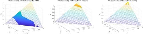
Suppose the portfolio $x^0=(0.31,0.69,0{)}^{\prime }$ includes the first two assets of Table 9 from the appendix, with random return ω given by the first two columns of this table. Let ${\mathcal{F}}_0\left(t\right)Pr\{\omega x^0<t\}$ be the risk profile of this portfolio and ${\mathcal{F}}_{\mathit{ref}}\left(t\right){\mathcal{F}}_0(t+\delta )$ (with constant $\delta =5\mathrm{\%}$) be the reference risk profile. The left figure in Figure 1 displays the shape of the non-convex disjoint feasible set of problem (5(5) $\begin{array}{rl}\mathrm{maximize}& f\left(x\right)\end{array}$(5) )–(6(6) $\begin{array}{rl}\text{subject to}& {\mathcal{F}}_x\left(t\right)\le {\mathcal{F}}_{\mathit{ref}}\left(t\right)\text{for all}t\in \mathbb{R}\mathrm{and}x\in X.\end{array}$(6) ) for this example. The figure in the middle gives an example of the feasible set of problem (5(5) $\begin{array}{rl}\mathrm{maximize}& f\left(x\right)\end{array}$(5) )–(6(6) $\begin{array}{rl}\text{subject to}& {\mathcal{F}}_x\left(t\right)\le {\mathcal{F}}_{\mathit{ref}}\left(t\right)\text{for all}t\in \mathbb{R}\mathrm{and}x\in X.\end{array}$(6) ), when a risk-free asset is infeasible. The right figure of Figure 1 corresponds to the case of a feasible risk-free portfolio.

When the distribution of returns ω is discrete (i.e. represented by scenarios), the distribution function ${\mathcal{F}}_x\left(t\right)$ of the portfolio return is discontinuous in x as a weighted sum of step-wise indicator functions, so the stochastic dominance constraints are represented by discontinuous functions. So generally, we deal with discontinuous optimization problems, which are a challenge for optimization theory. In particular, the constraints in these problems can be non-convex and disjoint. Our first step towards a solution of such problems is to eliminate constraints by a penalty method. However, the standard exact penalty methods that add a penalty term to the objective function is invalid in this case. In the next section we consider two new exact penalty methods, discontinuous and projective ones.

4.3. Exact discontinuous penalty functions

To find an optimal solution for problem (5(5) $\begin{array}{rl}\mathrm{maximize}& f\left(x\right)\end{array}$(5) )–(6(6) $\begin{array}{rl}\text{subject to}& {\mathcal{F}}_x\left(t\right)\le {\mathcal{F}}_{\mathit{ref}}\left(t\right)\text{for all}t\in \mathbb{R}\mathrm{and}x\in X.\end{array}$(6) ), we solve the problem (13) $\begin{array}{r}\underset{x\in X}{max}\left[F\right(x\left)\{\begin{array}{ll}f\left(x\right)& \mathrm{if}{G}_m\left(x\right)\le 0,\\ c-G_m\left(x\right)& \mathrm{else},\end{array}\right]\end{array}$(13) where $c<\underset{\{x\in X:G_m(x)\le 0\}}{sup}{f}_m\left(x\right)$, for example, $c=f\left(x_0\right)$ with $G_m\left(x_0\right)\le 0.$

Obviously, the global maximums of the problems (5(5) $\begin{array}{rl}\mathrm{maximize}& f\left(x\right)\end{array}$(5) )–(6(6) $\begin{array}{rl}\text{subject to}& {\mathcal{F}}_x\left(t\right)\le {\mathcal{F}}_{\mathit{ref}}\left(t\right)\text{for all}t\in \mathbb{R}\mathrm{and}x\in X.\end{array}$(6) ) and (13(13) $\begin{array}{r}\underset{x\in X}{max}\left[F\right(x\left)\{\begin{array}{ll}f\left(x\right)& \mathrm{if}{G}_m\left(x\right)\le 0,\\ c-G_m\left(x\right)& \mathrm{else},\end{array}\right]\end{array}$(13) ) coincide.

We can further remove the constraint $x\in X$ from problem (13(13) $\begin{array}{r}\underset{x\in X}{max}\left[F\right(x\left)\{\begin{array}{ll}f\left(x\right)& \mathrm{if}{G}_m\left(x\right)\le 0,\\ c-G_m\left(x\right)& \mathrm{else},\end{array}\right]\end{array}$(13) ) by subtracting the exact projective penalty term $\Vert x-{\pi }_X\left(x\right)\Vert$, where ${\pi }_X\left(x\right)$ is the projection of x on X, from the objective function (13(13) $\begin{array}{r}\underset{x\in X}{max}\left[F\right(x\left)\{\begin{array}{ll}f\left(x\right)& \mathrm{if}{G}_m\left(x\right)\le 0,\\ c-G_m\left(x\right)& \mathrm{else},\end{array}\right]\end{array}$(13) ), and solve the global problem (14) $\begin{array}{r}\underset{x\in {\mathbb{R}}^n}{max}\mathrm{\Phi }\left(x\right)F\left({\pi }_X\right(x\left)\right)-\Vert x-{\pi }_X\left(x\right)\Vert \end{array}$(14) instead.

4.4. Exact projective penalty functions

Let $x^0\in X$ be some feasible solution of problem (5(5) $\begin{array}{rl}\mathrm{maximize}& f\left(x\right)\end{array}$(5) )–(6(6) $\begin{array}{rl}\text{subject to}& {\mathcal{F}}_x\left(t\right)\le {\mathcal{F}}_{\mathit{ref}}\left(t\right)\text{for all}t\in \mathbb{R}\mathrm{and}x\in X.\end{array}$(6) ), i.e. $x^0\in X$ and $G_m\left(x^0\right)\le 0$. For any $x\in {\mathbb{R}}^n$ denote $x_{\lambda }=(1-\lambda )x^0+\lambda x$. Define a projection point (15) $\begin{array}{r}{p}_{G_m}\left(x\right)=\{\begin{array}{ll}x& \mathrm{if}{G}_m\left(x\right)\le 0,\\ x_{{\lambda }_x}& \mathrm{if}{G}_m\left(x\right)>0,\end{array}\end{array}$(15) where $\begin{array}{r}{\lambda }_x=sup\{\lambda \in [0,1]:G_m(x_{\lambda })\le 0\}.\end{array}$Now instead of the constrained problem (5(5) $\begin{array}{rl}\mathrm{maximize}& f\left(x\right)\end{array}$(5) )–(6(6) $\begin{array}{rl}\text{subject to}& {\mathcal{F}}_x\left(t\right)\le {\mathcal{F}}_{\mathit{ref}}\left(t\right)\text{for all}t\in \mathbb{R}\mathrm{and}x\in X.\end{array}$(6) ) consider the unconstrained problem (16) $\begin{array}{r}\underset{x\in {\mathbb{R}}^n}{max}\left[F_m\right(x)f_m\left(p_{G_m}\right({\pi }_X\left(x\right)\left)\right)-\Vert p_{G_m}({\pi }_X\left(x\right))-{\pi }_X(x)\Vert -\Vert x-{\pi }_X(x)\Vert ].\end{array}$(16) Similarly, instead of constrained problem (7(7) $\begin{array}{rl}\mathrm{maximize}& f\left(x\right)\end{array}$(7) )–(8(8) $\begin{array}{rl}\text{subject to}& {\mathcal{Q}}_{\mathit{ref}}\left(\alpha \right)\le {\mathcal{Q}}_x\left(\alpha \right)\text{for all}\alpha \in [0,1]\mathrm{and}x\in X.\end{array}$(8) ), we can consider the unconstrained problem (17) $\begin{array}{r}\underset{x\in {\mathbb{R}}^n}{max}\left[F_m\right(x)f_m\left(p_{H_m}\right({\pi }_X\left(x\right)\left)\right)-\Vert p_{H_m}({\pi }_X\left(x\right))-{\pi }_X(x)\Vert -\Vert x-{\pi }_X(x)\Vert ].\end{array}$(17) The exact projective penalty method was studied and tested in Norkin [1,42], Galvan [50]. The main features of the method are: it is exact, it does not require selection of the right penalty parameter, and it does not use the objective function values outside the feasible set. Also, for the considered portfolio reshaping problem, the exact projective penalty function can be found in a closed form.

By Norkin [1, Theorem 4.4], the global maximums of problems (5(5) $\begin{array}{rl}\mathrm{maximize}& f\left(x\right)\end{array}$(5) )–(6(6) $\begin{array}{rl}\text{subject to}& {\mathcal{F}}_x\left(t\right)\le {\mathcal{F}}_{\mathit{ref}}\left(t\right)\text{for all}t\in \mathbb{R}\mathrm{and}x\in X.\end{array}$(6) ) and (16(16) $\begin{array}{r}\underset{x\in {\mathbb{R}}^n}{max}\left[F_m\right(x)f_m\left(p_{G_m}\right({\pi }_X\left(x\right)\left)\right)-\Vert p_{G_m}({\pi }_X\left(x\right))-{\pi }_X(x)\Vert -\Vert x-{\pi }_X(x)\Vert ].\end{array}$(16) ) coincide, and, if the mapping $p_{G_m}\left({\pi }_X\right(x\left)\right)$ is continuous, also the local maximums of both problems coincide, i.e. the optimization problems are equivalent. The mapping $p_{G_m}\left({\pi }_X\right(x\left)\right)$ is continuous, if the feasible set is convex and the projection mapping (15(15) $\begin{array}{r}{p}_{G_m}\left(x\right)=\{\begin{array}{ll}x& \mathrm{if}{G}_m\left(x\right)\le 0,\\ x_{{\lambda }_x}& \mathrm{if}{G}_m\left(x\right)>0,\end{array}\end{array}$(15) ) uses an internal point $x^0$ of the feasible set of the considered problem. For example, a feasible risk-free portfolio can represent such point.

Remark 4.1

Computational aspects

The calculations of the projections $p_{G_m}(\cdot )$ and $p_{H_m}(\cdot )$ requires finding roots of the equations $\varphi \left(\lambda \right)G_m\left(x_{\lambda }\right)=0$ and $\psi \left(\lambda \right)H_m\left(x_{\lambda }\right)=0$. This requires multiple evaluations of the functions $\varphi \left(\lambda \right)$ and $\psi \left(\lambda \right)$, and hence, multiple construction of ${\mathcal{F}}_{x_{\lambda },m}\left(t\right)=Pr\{{\omega }^{\prime }{x}_{\lambda }\le t\}$ or ${\mathcal{Q}}_{x_{\lambda },m}\left(\alpha \right)$ for different portfolios $x_{\lambda }$. This may take considerable time in case of large number of observations m. However, in case of a specific feasible point, namely a risk-free (feasible) portfolio, these functions can be easily found through ${\mathcal{F}}_{x,m}\left(t\right)$ and ${\mathcal{Q}}_{x,m}\left(\alpha \right)$ as the following statements show.

Proposition 4.2

Let $x^0=(1,0,\dots ,0)$ be a risk-free portfolio with fixed return r, $x\in X$ be an arbitrary portfolio, with the random return $f(x,\omega )={\omega }^{\prime }x$, the return cumulative distribution function ${\mathcal{F}}_x\left(t\right)$, $t\in \mathbb{R}$, and the corresponding inverse (quantile) one ${\mathcal{Q}}_x\left(\alpha \right)$, $\alpha \in [0,1]$, $X=\{x\in {\mathbb{R}}^n:\sum _{i=1}^n{x}_i=1,x_i\ge 0,\text{ı}=1,\dots ,n\}$. Consider a mixed portfolio of the form $x_{\lambda }=\lambda x+(1-\lambda )x^0$, $\lambda \in [0,1]$. Its distribution function and inverse distribution function are expressed through ${\mathcal{F}}_x\left(t\right)$ and ${\mathcal{Q}}_x\left(\alpha \right)$ as $\begin{array}{r}{\mathcal{F}}_{x_{\lambda }}\left(t\right)={\mathcal{F}}_x\left(\right(t-(1-\lambda )r\left)/\lambda \right),\end{array}$and $\begin{array}{r}{\mathcal{Q}}_{x_{\lambda }}\left(\alpha \right)=\lambda {\mathcal{Q}}_x\left(\alpha \right)+(1-\lambda )r.\end{array}$

Proof.

Denote $f(x,\omega )={\omega }^{\prime }x$ and $f(x_{\lambda },\omega )={\omega }^{\prime }{x}_{\lambda }$. Then $\begin{array}{rl}{\mathcal{F}}_{x_{\lambda }}\left(t\right)& =Pr\left\{f\right(x_{\lambda },\omega )<t\}\\ & =Pr\left\{{\omega }^{\prime }\right(1-\lambda )x^0+\mathrm{\lambda f}(x,\omega )<t\}\\ & =Pr\left\{\right(1-\lambda )r+\mathrm{\lambda f}(x,\omega )<t\}\\ & =Pr\left\{f\right(x,\omega )<(t-(1-\lambda )r\left)/\lambda \right\}\\ & ={\mathcal{F}}_x\left(\right(t-(1-\lambda )r\left)/\lambda \right).\end{array}$Next, by definition, ${\mathcal{Q}}_{x_{\lambda }}\left(\alpha \right)$ is the optimal value of the optimization problem $\begin{array}{rl}& max\{t\in \mathbb{R}:{\mathcal{F}}_{x_{\lambda }}(t)\le \alpha \}\\ & =max\{t\in \mathbb{R}:Pr\{f(x_{\lambda },\omega )<t\le \alpha \}\\ & =max\{t\in \mathbb{R}:{\mathcal{F}}_x((t-(1-\lambda \left)r\right)/\lambda \le \alpha \}.\end{array}$With the variable $\tau =(t-(1-\lambda \left)r\right)/\lambda$, the latter problem is equivalent to $\begin{array}{r}max\{\mathrm{\lambda \tau }+(1-\lambda )r:{\mathcal{F}}_{x_{\lambda }}(\tau )\le \alpha \}.\end{array}$The optimal value of this problem equals the expression $\begin{array}{r}\lambda \underset{\tau \in \mathbb{R}}{sup}\{\tau :{\mathcal{F}}_x\left(\tau \right)\le \alpha \}+(1-\lambda )r=\lambda {\mathcal{Q}}_x\left(\alpha \right)+(1-\lambda )r={\mathcal{Q}}_{x_{\lambda }}\left(\alpha \right),\end{array}$which completes the proof.

The preceding proposition shows that the quantile function ${\mathcal{Q}}_{x_{\lambda }}\left(\alpha \right)$ of the mixed portfolio $x_{\lambda }=\lambda x+(1-\lambda )x^0$ is the weighted quantile function the return r of the risk-free portfolio $x^0$ and $Q_x\left(\alpha \right)$, the return quantile function of the portfolio x.

Thus, for a known risk-free feasible portfolio $x^0=(1,0,\dots ,0{)}^{\prime }$ with a fixed return r>0, the calculations can be reduced considerably. Indeed, we need to calculate only one CDF ${\mathcal{F}}_{x,m}(\cdot )$ and can re-use it for the CDFs ${\mathcal{F}}_{x_{\lambda },m}(\cdot )$ for different values of λ. In case of a discrete reference CDF ${\mathcal{F}}_{\mathit{ref}}\left(t\right)$ with jump points $({\mathcal{T}}_{\mathit{ref}},{\mathcal{A}}_{\mathit{ref}})=\left\{\right(t_1,{\alpha }_1),\dots ,(t_k,{\alpha }_k),\dots \}$, the projection $p_{H_m}\left(x\right)$ can be found in an analytical form as the following proposition states.

Proposition 4.3

Assume that ${\mathcal{Q}}_{\mathit{ref}}\left(1\right)<r$, then there exists a risk-free internal feasible portfolio $x^0$ with return r. Further, the projection $p_{H_m}\left(x\right)$ can be stated in the closed form $p_{H_m}\left(x\right)=(1-{\lambda }_x)x^0+{\lambda }_{x}x$, where $\begin{array}{r}{\lambda }_x=\{\begin{array}{ll}1,& \mathrm{if}{H}_m\left(x\right)\le 0,\\ \underset{\{\alpha \in {\mathcal{A}}_{\mathit{ref}}:{\mathcal{Q}}_x(\alpha )<{\mathcal{Q}}_{\mathit{ref}}(\alpha \left)\right\}}{min}\frac{{\mathcal{Q}}_{\mathit{ref}}\left(\alpha \right)-r}{{\mathcal{Q}}_x\left(\alpha \right)-r},& \mathrm{if}{H}_m\left(x\right)>0.\end{array}\end{array}$

Proof.

It holds that ${\mathcal{Q}}_{\mathit{ref}}\left(\alpha \right)\le {\mathcal{Q}}_{\mathit{ref}}\left(1\right)<r={\mathcal{Q}}_{x^0}\left(\alpha \right)$, i.e. the risk-free portfolio $x^0=(1,0,\dots ,0{)}^{\mathrm{\prime }}$ is feasible and internal.

For $H_m\left(x\right)\le 0$ we have, by definition, $p_{H_m}\left(x\right)=x$. So assume that $H_m\left(x\right)>0$. Consider the portfolios $x_{\lambda }=(1-\lambda )x^0+\mathrm{\lambda x}$, $\lambda \in [0,1]$, and the function $\begin{array}{rl}{h}_x(\alpha ,\lambda )& ={\mathcal{Q}}_{\mathit{ref}}\left(\alpha \right)-{\mathcal{Q}}_{x_{\lambda }}\left(\alpha \right)\\ & ={\mathcal{Q}}_{\mathit{ref}}\left(\alpha \right)-r-\lambda \left({\mathcal{Q}}_x\right(\alpha )-r).\end{array}$For $\alpha \in {\mathcal{A}}_{\mathit{ref}}$ such that ${\mathcal{Q}}_x\left(\alpha \right)<{\mathcal{Q}}_{\mathit{ref}}\left(\alpha \right)$ it holds that $h_x(\alpha ,1)>0$ and $h_x(\alpha ,0)<0$ and the function $h_x(\alpha ,\cdot )$ is linear strictly monotone. So the projection corresponds to the minimal λ such $h_x(\alpha ,\lambda )\ge 0$, that is to ${\lambda }_x$, $\begin{array}{r}{\lambda }_x=\underset{\{\alpha \in {\mathcal{A}}_{\mathit{ref}}:{\mathcal{Q}}_x(\alpha )<{\mathcal{Q}}_{\mathit{ref}}(\alpha \left)\right\}}{min}\frac{{\mathcal{Q}}_{\mathit{ref}}\left(\alpha \right)-r}{{\mathcal{Q}}_x\left(\alpha \right)-r},\end{array}$which completes the proof.

The proposition shows that given the conditions, the feasible set $\{x\in X:H_m(x)\le 0\}$ has a star shape with respect to the feasible point $x^0$ that represents a risk-free portfolio.

If ${\mathcal{Q}}_x\left(\alpha \right)$, $\alpha \in {\mathcal{A}}_{\mathit{ref}}$, are continuous functions in x, then, given the conditions of the preceding proposition, ${\lambda }_x$ is continuous. Hence, the projection mapping $p_m\left(x\right)={\lambda }_{x}x+(1-{\lambda }_x)x^0$ is also continuous. It follows from [1, Theorem 4.4] that the problems (7(7) $\begin{array}{rl}\mathrm{maximize}& f\left(x\right)\end{array}$(7) )–(8(8) $\begin{array}{rl}\text{subject to}& {\mathcal{Q}}_{\mathit{ref}}\left(\alpha \right)\le {\mathcal{Q}}_x\left(\alpha \right)\text{for all}\alpha \in [0,1]\mathrm{and}x\in X.\end{array}$(8) ) and (17(17) $\begin{array}{r}\underset{x\in {\mathbb{R}}^n}{max}\left[F_m\right(x)f_m\left(p_{H_m}\right({\pi }_X\left(x\right)\left)\right)-\Vert p_{H_m}({\pi }_X\left(x\right))-{\pi }_X(x)\Vert -\Vert x-{\pi }_X(x)\Vert ].\end{array}$(17) ) are equivalent.

5. Numerical optimization of discontinuous penalty functions

In this section, we consider a numerical method for the optimization of generally discontinuous functions $G_m\left(x\right)$, $H_m\left(x\right)$ and $F_m\left(x\right)$ in (11(11) $\begin{array}{r}\underset{x\in X}{min}{G}_m\left(x\right).\end{array}$(11) )–(17(17) $\begin{array}{r}\underset{x\in {\mathbb{R}}^n}{max}\left[F_m\right(x)f_m\left(p_{H_m}\right({\pi }_X\left(x\right)\left)\right)-\Vert p_{H_m}({\pi }_X\left(x\right))-{\pi }_X(x)\Vert -\Vert x-{\pi }_X(x)\Vert ].\end{array}$(17) ). The idea consists in sequential approximations of the original function by smooth (averaged) ones and optimizing the latter by stochastic optimization methods. For this we develop a stochastic finite-difference estimates of gradients of the smoothed functions. Although the successive smoothing method has certain global optimization abilities (as discussed in [42]), to strengthen this property we embed it as a local optimizer into some branch and bound scheme.

The problem setting satisfies the following conditions, which justify the tools employed to numerically solve the problem.

1. The original optimization problems are correctly set, i.e. they have feasible and optimal solutions. The Lemmas 3.1, 3.3 and 3.4 ensure this assumption.

2. The original constrained problems are transformed to unconstrained ones and this transformation are assumed to be exact. The exact discontinuous and exact projective penalty methods discussed in Section 4 and in [1] provide this transformation.

3. Penalty functions are approximated by a sequence of smoothed functions, and this sequence epi-converges to the target penalty function. The so-called strongly lower semicontinuous functions (see Definition 5.1 and Theorem 5.4 in Subsection 5.1 below) ensure this property.

4. The level sets of the penalty and the smoothed functions are uniformly bounded. This property is provided by penalty term $\Vert x-{\pi }_X\left(x\right)\Vert$ in (16(16) $\begin{array}{r}\underset{x\in {\mathbb{R}}^n}{max}\left[F_m\right(x)f_m\left(p_{G_m}\right({\pi }_X\left(x\right)\left)\right)-\Vert p_{G_m}({\pi }_X\left(x\right))-{\pi }_X(x)\Vert -\Vert x-{\pi }_X(x)\Vert ].\end{array}$(16) ) and (17(17) $\begin{array}{r}\underset{x\in {\mathbb{R}}^n}{max}\left[F_m\right(x)f_m\left(p_{H_m}\right({\pi }_X\left(x\right)\left)\right)-\Vert p_{H_m}({\pi }_X\left(x\right))-{\pi }_X(x)\Vert -\Vert x-{\pi }_X(x)\Vert ].\end{array}$(17) ) related to projection on the convex set X.

5. For the unconstrained minimization of smoothed functions we apply stochastic finite-difference gradient method in a combination of a branch and bound method, which are assumed to approximately find their global minimums. Both applied methods are heuristic, their structure and convergence properties are discussed in Subsection 5.2 below.

6. Convergence of the approximate global minimums to global minimums of the penalty function (on a subset, where penalty function values can be approached through its continuity points) is guaranteed by properties of epi-convergence, cf. [51, Theorem 7.33].

5.1. Averaged functions

We limit the consideration to the case of the so-called strongly lower semicontinuous functions.

Definition 5.1

Strongly lower semicontinuous functions, cf. [43]

A function $F:{\mathbb{R}}^n\to \mathbb{R}$ is called lower semicontinuous (lsc) at a point x, if $\begin{array}{r}\underset{\nu \to \mathrm{\infty }}{lim inf}F\left(x^{\nu }\right)\ge F\left(x\right)\end{array}$for all sequences $x^k\to x$.

A function $F:{\mathbb{R}}^n\to \mathbb{R}$ is called strongly lower semicontinuous (strongly lsc) at a point x, if it is lower semicontinuous at x and there exists a sequence $x^k\to x$ such that it is continuous at $x^k$ (for all $x^k$) and $F\left(x^k\right)\to F\left(x\right)$. A function F is called strongly lower semicontinuous (strongly lsc) on $X\subseteq {\mathbb{R}}^n$, if this is the case for all $x\in X$.

The property of strong lower semi-continuity is preserved under continuous transformations. Some further properties of these functions are discussed in [52].

If the function $F:{\mathbb{R}}^n\to \mathbb{R}$ is continuous almost everywhere (i.e. it is discontinuous on some set of measure zero), then its (lower) regularization (18) $\begin{array}{r}\hat{F}\left(x\right)lim inf\left\{F\right(x^k):x^k\to x,F\text{is continuous at}{x}^k\}\end{array}$(18) is strongly lower semicontinuous and coincides with F almost everywhere.

The averaged functions obtained from the original non-smooth or discontinuous function by convolution with some kernel have smoother characteristics. For this reason, they are often used in optimization theory (see [43,53] and references therein).

Definition 5.2

The set (family) of bounded and integrable functions $\{{\psi }_{\theta }:{\mathbb{R}}^n\to R_{+},\theta \in {\mathbb{R}}_{+}\}$ satisfying for any $ϵ>0$ the conditions $\begin{array}{r}\underset{\theta \to 0}{lim}{\int }_{ϵ\mathbf{B}}{\psi }_{\theta }\left(z\right)\mathrm{d}z=1,\mathbf{B}\{x\in {\mathbb{R}}^n:\Vert x\Vert \le 1\},\end{array}$is called a family of mollifiers. The kernels $\left\{{\psi }_{\theta }\right\}$ are said to be smooth if the functions ${\psi }_{\theta }(\cdot )$ are continuously differentiable.

A function $F:{\mathbb{R}}^n\to {\mathbb{R}}^1$ is called bounded at infinity if there are positive numbers C and r such that $|F\left(x\right)|\le C$ for all x with $\Vert x\Vert \ge r$.

Given a locally integrable, bounded at infinity, function $F:{\mathbb{R}}^n\to {\mathbb{R}}^1$ and a family of smoothing kernels $\left\{{\psi }_{\theta }\right\}$, the associated family of averaged functions $\{F_{\theta }:\theta \in {\mathbb{R}}_{+}\}$ is (19) $\begin{array}{r}{F}_{\theta }\left(x\right){\int }_{{\mathbb{R}}^n}F(x+z){\psi }_{\theta }\left(z\right)\mathrm{d}z={\int }_{{\mathbb{R}}^n}F\left(z\right){\psi }_{\theta }(z-x)\mathrm{d}z.\end{array}$(19) Smoothing kernels can have an unlimited support $\mathrm{supp}{\psi }_{\theta }=\{x:{\psi }_{\theta }(x)>0\}$. To ensure the existence of the integrals (19(19) $\begin{array}{r}{F}_{\theta }\left(x\right){\int }_{{\mathbb{R}}^n}F(x+z){\psi }_{\theta }\left(z\right)\mathrm{d}z={\int }_{{\mathbb{R}}^n}F\left(z\right){\psi }_{\theta }(z-x)\mathrm{d}z.\end{array}$(19) ), we assume that the function F is bounded at infinity. We can always assume this property if we are interested in the behaviour of F within some bounded area. If $\mathrm{supp}{\psi }_{\theta }\to 0$ for $\theta \to 0$, then this assumption is superfluous.

For example, a family of kernels can be as follows. Let ψ be some probability density function with bounded support $\mathrm{supp}\psi$, a positive numerical sequence $\{{\theta }_{\nu }:\nu =1,2,\dots \}$ tending to 0 as $\nu \to \mathrm{\infty }$. Then the smoothing kernels on ${\mathbb{R}}^n$ can be taken as $\begin{array}{r}{\psi }_{{\theta }_{\nu }}\left(z\right)\frac{1}{({\theta }_{\nu }{)}^n}\psi \left(z/{\theta }_{\nu }\right),\end{array}$where ${\theta }_{\nu }$ is a bandwidth.

If the function F is not continuous, then we cannot expect the averaged functions $F_{\theta }\left(x\right)$ to converge to F uniformly. But we don't need that. We need such a convergence of the averaged functions $F_{\theta }\left(x\right)$ to F that guarantees the convergence of the minima of $F_{\theta }\left(x\right)$ to the minima of F. This property is guaranteed by the so-called epi-convergence of functions.

Definition 5.3

Epi-convergence, cf. Rockafellar and Wets [54]

A sequence of functions $\{F^{\nu }:{\mathbb{R}}^n\to \overline{\mathbb{R}},\nu \in \mathbb{N}\}$ epi-converges to a function $F:{\mathbb{R}}^n\to \overline{\mathbb{R}}$ at a point x, iff

1. $\underset{\nu \to \mathrm{\infty }}{lim inf}{F}^{\nu }\left(x^{\nu }\right)\ge F\left(x\right)$ for all $x^{\nu }\to x$ and

2. $\underset{\nu \to \mathrm{\infty }}{lim inf}{F}^{\nu }\left(x^{\nu }\right)=F\left(x\right)$ for some sequence $x^{\nu }\to x$.

The sequence $\left\{F^{\nu }\right\}$ epi-converges to F, if this is the case at every point $x\in {\mathbb{R}}^n$.

Theorem 5.4

Epi-convergence of averaged functions, cf. [43], Theorem 3.7 and [51], Example 7.19

For a strongly lower semicontinuous locally integrable function $F:{\mathbb{R}}^n\to {\mathbb{R}}^1$, any associated sequence of averaged functions $\{F^{\nu }=F_{{\theta }_{\nu }}:{\theta }_{\nu }\in {\mathbb{R}}_{+}\}$ epi-converges to F as ${\theta }_{\nu }\downarrow 0$.

Note that in the optimization problem without constraints it follows that $\begin{array}{r}\underset{\nu }{lim}\left(\underset{x}{inf}{F}^{\nu }\right)=\underset{x}{inf}F,\end{array}$cf. [51, Theorem 7.33].

We remark that for almost everywhere continuous function F, the corresponding averaged functions $F_{{\theta }_{\nu }}$ epi-converge to its regularization $\hat{F}$ defined in (18(18) $\begin{array}{r}\hat{F}\left(x\right)lim inf\left\{F\right(x^k):x^k\to x,F\text{is continuous at}{x}^k\}\end{array}$(18) ).

To optimize discontinuous functions, we approximate them with averaged functions. The convolution of a discontinuous function with the corresponding kernel (probability density) improves analytical properties of the resulting function, but increases the computational complexity of the problem, since it transforms the deterministic function into an expectation, which is a multidimensional integral. This transformation of the problem, which involves probability measures, naturally links to well-studied and well-established methods in stochastic optimization.

We can consider smoothed functions obtained by employing differentiable kernel with unbounded support, for example the Gaussian kernel given by the probability density $\begin{array}{r}\psi \left(y\right)=(2\pi {)}^{-n/2}{\mathrm{e}}^{-\Vert y{\Vert }^2/2}.\end{array}$Consider the family $\begin{array}{r}{F}_{\theta }\left(x\right)={\int }_{{\mathbb{R}}^n}F(x+\mathrm{\theta y})\psi \left(y\right)\mathrm{d}y=\frac{1}{{\theta }^n}{\int }_{{\mathbb{R}}^n}F\left(z\right)\psi \left(\frac{z-x}{\theta }\right)\mathrm{d}z,\theta >0,\end{array}$of averaged functions. Suppose that F is globally bounded (one may even assume that $|F\left(x\right)|\le {\gamma }_1+{\gamma }_2\Vert x{\Vert }^{{\gamma }_3}$ with some non-negative constants ${\gamma }_1$, ${\gamma }_2$ and ${\gamma }_3$). Then for the strongly lsc function F, the average functions $F_{\theta }$ epi-converge to F as $\theta \downarrow 0$ and each function $F_{\theta }$ is analytical with gradient (cf. Stein's lemma) $\begin{array}{rl}\mathrm{\nabla }{F}_{\theta }\left(x\right)& =\frac{1}{{\theta }^{n+2}}{\int }_{{\mathbb{R}}^n}F\left(z\right)\psi \left(\frac{z-x}{\theta }\right)(z-x)\mathrm{d}z=\frac{1}{\theta }{\int }_{{\mathbb{R}}^n}F(x+\theta y)\psi \left(y\right)y\mathrm{d}y\\ & =-\frac{1}{\theta }{\int }_{{\mathbb{R}}^n}F(x-\mathrm{\theta y})\psi \left(y\right)y\mathrm{d}y=\frac{1}{\theta }{\int }_{{\mathbb{R}}^n}\left(F\right(x+\mathrm{\theta y})-F(x\left)\right)\psi \left(y\right)y\mathrm{d}y\\ & =\frac{1}{2\theta }{\int }_{{\mathbb{R}}^n}\left(F\right(x+\mathrm{\theta y})-F(x-\mathrm{\theta y}\left)\right)\psi \left(y\right)y\mathrm{d}y,\end{array}$or (20) $\begin{array}{r}\mathrm{\nabla }{F}_{\theta }\left(x\right)={\mathbb{E}}_{\eta }\frac{1}{\theta }\left(F\right(x+\mathrm{\theta \eta })-F(x\left)\right)\eta ={\mathbb{E}}_{\eta }\frac{1}{2\theta }\left(F\right(x+\mathrm{\theta \eta })-F(x-\mathrm{\theta \eta }\left)\right)\eta ,\end{array}$(20) where the random vector η follows the standard normal distribution and ${\mathbb{E}}_{\eta }$ is the mathematical expectation over η.

It follows that the random vector (21) $\begin{array}{r}{\xi }_{\theta }(x,\eta )=\frac{\eta }{2\theta }\left(F\right(x+\mathrm{\theta \eta })-F(x-\mathrm{\theta \eta }\left)\right)\end{array}$(21) with Gaussian random variable η is an unbiased random estimate of the gradient $\mathrm{\nabla }{F}_{\theta }\left(x\right)$.

5.2. Stochastic methods for minimization of discontinuous penalty functions

Consider a problem of constrained minimization of a generally discontinuous function subject to a box or other convex constraints. The target problems are (11(11) $\begin{array}{r}\underset{x\in X}{min}{G}_m\left(x\right).\end{array}$(11) )–(17(17) $\begin{array}{r}\underset{x\in {\mathbb{R}}^n}{max}\left[F_m\right(x)f_m\left(p_{H_m}\right({\pi }_X\left(x\right)\left)\right)-\Vert p_{H_m}({\pi }_X\left(x\right))-{\pi }_X(x)\Vert -\Vert x-{\pi }_X(x)\Vert ].\end{array}$(17) ).

Such problems can be solved, e.g. by collective random search algorithms. In this section, we develop stochastic quasi-gradient algorithms to solve these problems.

A problem of constrained optimization can be reduced to the problem of unconstrained optimization of a coercive function $F\left(x\right)$ by using non-smooth or discontinuous penalty functions as described in [1,42,50] (for the case of the present paper see Section 4).

Suppose the function $F\left(x\right)$ is strongly lower semicontinuous. In view of Theorem 5.4, it is always possible to construct a sequence of smoothed averaged functions $F_{{\theta }_{\nu }}$ that epi-converges to F. Due to this property, the global minima of $F_{{\theta }_{\nu }}$ converge to the global minima of F as ${\theta }_{\nu }\to 0$. Convergence of local minima was studied in [43].

Let us consider some procedures for optimizing the function F using approximating averaged functions $F_{{\theta }_{\nu }}$.

Suppose one can find the global minima $\left\{x^{\nu }\right\}$ of the functions $F_{{\theta }_{\nu }}$, $\nu =0,1,\dots$. Then any limit point of the sequence $\left\{x^{\nu }\right\}$ is a global minimum of the function F. However, finding global minima of $F_{{\theta }_{\nu }}$ can be a quite difficult task, so consider the following method.

The successive stochastic smoothing method, cf. [42]

The method sequentially minimizes a sequence of smoothed functions $F_{{\theta }_{\nu }}$ with decreasing smoothing parameter ${\theta }_{\nu }\downarrow 0$. The sequence of approximations $x^{\nu }$ is constructed by implementing the following steps (cf. [42]).

The successive smoothing method as a local optimizer.

1. Initialization. Fix a box $[\mathrm{lb},\mathrm{ub}]$ with lower (lb) and upper (ub) bounds on the problem variables, select a number N of (decreasing) smoothing steps and a decreasing rate $\alpha \in [1/2,1)$; K is the number of iterations of the Nemirovski-Yudin method (NYM), select a starting (maximal) smoothing parameter ${\theta }_1$, e.g. ${\theta }_1=\Vert \mathrm{ub}-\mathrm{lb}\Vert .$ Select a (random) starting point $x^0\in (\mathrm{lb},\mathrm{ub})$. Set $\nu =1$, the initial smoothing iteration count.

2. Smoothing iterations. For a fixed smoothing parameter ${\theta }_{\nu }$, $\nu \ge 1,$ minimize the smoothed function $F_{{\theta }_{\nu }}$ by some stochastic optimization method with the use of the initial point $x^{\nu }$ and finite-difference stochastic gradients (21(21) $\begin{array}{r}{\xi }_{\theta }(x,\eta )=\frac{\eta }{2\theta }\left(F\right(x+\mathrm{\theta \eta })-F(x-\mathrm{\theta \eta }\left)\right)\end{array}$(21) ) to find the next approximation $x^{\nu +1}$. For example, this can be done by the following stochastic optimization algorithm.

   1. Initialization of the Nemirovski-Yudin method (NYM). Fix $m\ge 1$ the sample size for the gradient estimation. Set k=1, $y^1=z^1=x^{\nu }$.

   2. Batch estimation of the gradient $\mathrm{\nabla }{F}_{{\theta }_{\nu }}\left(y^k\right)$. Sample independent, normally distributed directions ${\eta }^1,\dots ,{\eta }^m\in {\mathbb{R}}^n$ and calculate the current estimate of $\mathrm{\nabla }{F}_{{\theta }_{\nu }}\left(y^k\right)$ by employing (21(21) $\begin{array}{r}{\xi }_{\theta }(x,\eta )=\frac{\eta }{2\theta }\left(F\right(x+\mathrm{\theta \eta })-F(x-\mathrm{\theta \eta }\left)\right)\end{array}$(21) ) as $\begin{array}{r}{\xi }_{{\theta }_{\nu }}\left(y^k\right)=\sum _{i=1}^m\frac{1}{2{\theta }_{\nu }}\left(F\right(y^k+{\theta }_{\nu }{\eta }^i)-F(y^k-{\theta }_{\nu }{\eta }^i\left)\right){\eta }^i.\end{array}$

   3. Itarations of NYM: $\begin{array}{rl}{y}^{k+1}& ={\mathrm{\Pi }}_{[\mathrm{lb},\mathrm{ub}]}(y^k-{\rho }_k\frac{{\xi }_{{\theta }_{\nu }}\left(y^k\right)}{\Vert {\xi }_{{\theta }_{\nu }}\left(y^k\right)\Vert +ϵ}),{\rho }_k={\theta }_{\nu }/\sqrt{k},ϵ>0,\\ z^{k+1}& =(1-\frac{{\rho }_k}{\sum _{i=1}^k{\rho }_i})z^k+\left(\frac{{\rho }_k}{\sum _{i=1}^k{\rho }_i}\right)y^{k+1},\end{array}$where ${\mathrm{\Pi }}_{[\mathrm{lb},\mathrm{ub}]}(\cdot )$ is the projection operator on the box $[\mathrm{lb},\mathrm{ub}]$.

   4. Stopping of NYM. Increase k by 1. If k<K, then go to (ii)b, else continue with 5.2.

3. Gelfand–Zetlin–Nesterov step. Set $\begin{array}{r}{x}^{\nu +1}=z^{k+1}+\lambda (z^{k+1}-z^k),\lambda \in [0,1),\text{e.g.}\lambda =\mathrm{0.8.}\end{array}$

4. Transition to the next less smoothing step (or stop). Increase the smoothing iteration number ν by 1, decrease the smoothing parameter ${\theta }_{\nu +1}=\alpha \cdot {\theta }_{\nu }$. If $\nu <N$, go to step (ii), else return an approximate solution $x^{\nu }$ of the optimization problem.

The successive smoothing method described above starts with a more smooth function that disregards the fine structure of the objective to find the most promising regions in the search space before gradually making the approximation more exact. The successive smoothing with gradual vanishing degree of smoothing distinguishes our method from other smoothing methods, which use fixed smoothing for minimization of non-smooth functions. In our method we allocate a fixed number K of iterations to minimize a smoothed function $F_{{\theta }_{\nu }}(\cdot )$. For a particular case K=1 (and $\lambda =0$), the convergence rate of the successive smoothing method on the class of Lipschitz non-smooth convex functions was studied in [55]. Roughly speaking, the rate of convergence (in function) of the method is proportional to the range of the function on the feasible set multiplied by factor $\sqrt{n/\left(\mathrm{mN}\right)}$, where n is the dimension of the space, m is the number of finite differences for estimation of gradients. This method stops after N smoothing iterations. The other practical stopping rule is to stop computations, if there is no progress of the algorithm after several iterations.

For the minimization of the smoothed function $F_{\theta }$ under fixed $\theta ={\theta }_{\nu }$, one can apply any (not necessary NY mirror descent [56] but, e.g. a stochastic version of the Nesterov's method [57]) stochastic finite-difference optimization method based on the finite difference representations (20(20) $\begin{array}{r}\mathrm{\nabla }{F}_{\theta }\left(x\right)={\mathbb{E}}_{\eta }\frac{1}{\theta }\left(F\right(x+\mathrm{\theta \eta })-F(x\left)\right)\eta ={\mathbb{E}}_{\eta }\frac{1}{2\theta }\left(F\right(x+\mathrm{\theta \eta })-F(x-\mathrm{\theta \eta }\left)\right)\eta ,\end{array}$(20) ), (21(21) $\begin{array}{r}{\xi }_{\theta }(x,\eta )=\frac{\eta }{2\theta }\left(F\right(x+\mathrm{\theta \eta })-F(x-\mathrm{\theta \eta }\left)\right)\end{array}$(21) ) of the gradients of the smoothed function. In the described NY algorithm, the local optimization of $F_{\theta }$ stops after K iterations.

One more possible stopping rule is based on estimating gradients $\mathrm{\nabla }{F}_{\theta }\left(x\right)$ during the iterative optimization process. In general, this is a rather complicated and time-consuming procedure that requires calculation of multidimensional integrals. However, such asymptotically consistent estimates can be constructed in parallel with the construction of the main minimization sequence by using the following so-called averaging procedure [45,58,59].

Consider the stochastic optimization procedure $\begin{array}{rl}{x}^{k+1}& =x^k-{\rho }_k{z}^k,z^0={\xi }_{\theta }(x^0,{\eta }^0),x^0\in {\mathbb{R}}^n,\\ z^{k+1}& =z^k-{\lambda }_k(z^k-{\xi }_{\theta }(x^k,{\eta }^k\left)\right),k=0,1,\dots ,\end{array}$for an iterative optimization of a function $F_{\theta }\left(x\right)$ and parallel evaluation of its gradients $\mathrm{\nabla }{F}_{\theta }\left(x\right)$, where the vectors ${\xi }_{\theta }(x^k,\eta )$ are given by (21(21) $\begin{array}{r}{\xi }_{\theta }(x,\eta )=\frac{\eta }{2\theta }\left(F\right(x+\mathrm{\theta \eta })-F(x-\mathrm{\theta \eta }\left)\right)\end{array}$(21) ). For the conditional expectations it holds that $\mathbb{E}\left({\xi }_{\theta }\right(x^k,{\eta }^k)\mid x^k)=\mathrm{\nabla }{F}_{\theta }\left(x^k\right)$. Let the numbers ${\rho }_k$, ${\lambda }_k$ satisfy the conditions $\begin{array}{rl}0& \le {\lambda }_k\le 1,\underset{k}{lim}{\lambda }_k=0,\sum _{k=0}^{\mathrm{\infty }}{\lambda }_k=+\mathrm{\infty },\sum _{k=0}^{\mathrm{\infty }}{\lambda }_k^2<+\mathrm{\infty },\mathrm{and}\\ \underset{k}{lim}\frac{{\rho }_k}{{\lambda }_k}& =0.\end{array}$Then, with probability one, it holds (cf. Ermoliev [58, Theorem V.8]) that $\begin{array}{r}{z}^k-\mathrm{\nabla }{F}_{\theta }\left(x^k\right)\to 0\mathrm{as}k\to \mathrm{\infty }.\end{array}$If $\Vert \mathrm{\nabla }{F}_{{\theta }_{\nu }}\left(x^{\nu }\right)\Vert \le {ϵ}_{\nu }\to 0$, then, by results of [43,45,60], the constructed sequence $x^{\nu }$ asymptotically converges to the set, which satisfies necessary optimality conditions for F. Some other stopping rules for stochastic gradient methods are discussed, e.g. in [61].

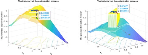
Figure 2 provides a graphical illustration of the performance of the successive smoothing method on problem (14(14) $\begin{array}{r}\underset{x\in {\mathbb{R}}^n}{max}\mathrm{\Phi }\left(x\right)F\left({\pi }_X\right(x\left)\right)-\Vert x-{\pi }_X\left(x\right)\Vert \end{array}$(14) ).

Figure 2. Illustration of the smoothing method performance on two asset (1,2) portfolio selection. Examples of the trajectories of the method for different discontinuous penalties. $x_{\mathit{ref}}=(x_1=0.3,x_2=0.7)$, $\delta =0.05$.

Global optimization issues.

The optimization problems under consideration (5(5) $\begin{array}{rl}\mathrm{maximize}& f\left(x\right)\end{array}$(5) )–(6(6) $\begin{array}{rl}\text{subject to}& {\mathcal{F}}_x\left(t\right)\le {\mathcal{F}}_{\mathit{ref}}\left(t\right)\text{for all}t\in \mathbb{R}\mathrm{and}x\in X.\end{array}$(6) ) and (7(7) $\begin{array}{rl}\mathrm{maximize}& f\left(x\right)\end{array}$(7) )–(8(8) $\begin{array}{rl}\text{subject to}& {\mathcal{Q}}_{\mathit{ref}}\left(\alpha \right)\le {\mathcal{Q}}_x\left(\alpha \right)\text{for all}\alpha \in [0,1]\mathrm{and}x\in X.\end{array}$(8) ) are challenging, they are non-convex and multi-extremal, discontinuous, disconnected and constrained. So we apply a number of different techniques to tackle and solve them.

To remove discontinuous constraints, we use exact discontinuous penalty functions, and to remove structural portfolio constraints and bound constraints, we apply exact projective penalty functions, cf. [1,42,50].

In the case of multi-extremal problems (as in Figure 3) we employ a version of the branch and bound method [1] with the successive smoothing method as a local minimizer (in [1], the successive quadratic approximation method was used as a local optimizer).

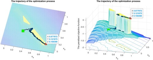
Figure 3. Illustration of the smoothing method performance on two asset (4,9) portfolio selection. Example of the trajectory of the method for non-connected feasible set. $x_{\mathit{ref}}=(x_4=0.3,x_9=0.7)$, $\delta =0.05$. The green is the starting point, the red is the final one.

To solve problem (11(11) $\begin{array}{r}\underset{x\in X}{min}{G}_m\left(x\right).\end{array}$(11) )–(17(17) $\begin{array}{r}\underset{x\in {\mathbb{R}}^n}{max}\left[F_m\right(x)f_m\left(p_{H_m}\right({\pi }_X\left(x\right)\left)\right)-\Vert p_{H_m}({\pi }_X\left(x\right))-{\pi }_X(x)\Vert -\Vert x-{\pi }_X(x)\Vert ].\end{array}$(17) ), we apply the following branch and bound (cut) algorithm acting in a box $[\mathrm{lb},\mathrm{ub}]\subset {\mathbb{R}}^n$.

The Branch & Bound algorithm.

Initialization.	Set the initial partition ${\mathcal{P}}_0=\{X=[\mathrm{lb},\mathrm{ub}\left]\right\}$, select a random starting point ${\tilde{x}}^0\in X$ and apply some local optimization algorithm $\mathcal{A}$ to the problem under consideration. As result, we find a better point ${\overline{x}}^0\in X$ such that $F\left({\overline{x}}^0\right)<F\left({\tilde{x}}^0\right)$. Set the B&B iteration count k=0. Set tolerances $ϵ>0$ and $\delta >0$. Set the integer stopping parameter $p\ge 2.$
B&B iteration.	Suppose at iteration k we have partition ${\mathcal{P}}_k=\{X_i:i=1,\dots ,N_k\}$ of the set $X={\cup }_{i=1}^{N_k}{X}_i$ consisting of smaller boxes $X_i$. For each $X_i$, there is a known feasible point ${\overline{x}}^i\in X_i$ and the corresponding value $F\left({\overline{x}}^i\right)$, $V_k=\underset{1\le i\le N_k}{min}F\left({\overline{x}}^i\right)$. Set ${\mathcal{P}}_{k+1}=\mathrm{\varnothing }$. For each such set $X_i\in {\mathcal{P}}_k$ choose a random starting point ${\tilde{x}}^i$ and apply some local optimization algorithm (e.g. the successive smoothing one) to the problem $\underset{x\in X_i}{min}F\left(x\right)$ to find a better point ${\overline{\overline{x}}}^i\in X_i$, $F\left({\overline{\overline{x}}}^i\right)<F\left({\tilde{x}}^i\right)$. If the values $F\left({\overline{x}}^i\right)$ and $F\left({\overline{\overline{x}}}^i\right)$ are sufficiently different, say $\Vert F\left({\overline{x}}^i\right)-F\left({\overline{\overline{x}}}^i\right)\Vert \ge ϵ$, or the points ${\overline{\overline{x}}}^i$ and ${\overline{x}}^i$ are sufficiently distinct, $\Vert {\overline{\overline{x}}}^i-{\overline{x}}^i\Vert \ge \delta$, we subdivide the box $X_i=X_i^{\mathrm{\prime }}\cup X_i^{\mathrm{\prime \prime }}$ into two subboxes $X_i^{\mathrm{\prime }}$ and $X_i^{\mathrm{\prime \prime }}$ so that ${\overline{x}}^i\in X_i^{\mathrm{\prime }}$ and ${\overline{\overline{x}}}^i\in X_i^{\mathrm{\prime \prime }}$. In this case, the partition ${\mathcal{P}}_{k+1}$ is updated by adding the successors $X_i^{\mathrm{\prime }}$ and $X_i^{\mathrm{\prime \prime }}$, i.e. ${\mathcal{P}}_{k+1}{\mathcal{P}}_{k+1}\cup X_i^{\mathrm{\prime }}\cup X_i^{\mathrm{\prime \prime }}.$ Otherwise, if the values $F\left({\overline{x}}^i\right)$ and $F\left({\overline{\overline{x}}}^i\right)$ and points ${\overline{\overline{x}}}^i$ and ${\overline{x}}^i$ are close, the set $X_i\ni {\overline{x}}^i$ goes unchanged to the updated partition ${\mathcal{P}}_{k+1}{\mathcal{P}}_{k+1}\cup X_i$. When all elements $X_i\in {\mathcal{P}}_k$ are examined in this way, i.e. the new partition ${\mathcal{P}}_{k+1}$ with elements $X_i,i=1,\dots ,N_{k+1}$, and points ${\overline{x}}_i\in X_i$ has been constructed, we modify the achieved record value, $V_{k+1}=\underset{1\le i\le N_{k+1}}{min}F\left({\overline{x}}^i\right)$.
Check for the stop.	If there is no progress of the B&B method during p B&B iterations, i.e. $V_{k+1}=V_{k+1-p}$, then stop; otherwise, repeat the B&B iteration.

Remark 5.5

The described B&B aims at subdividing a non-convex multiextremal problem into sub-problems, each containing only one local minimum. To prevent the method from early stop, two mechanisms are used. First, the stopping parameter $p\ge 2$ is introduced: the method stops after p unproductive B&B iterations. In all numerical experiments, p=5 was sufficient to find the global minimum. Second, for each new run of the local minimizer, a random starting point is used, that increases the probability of finding a new local minimum of the sub-problem.

Let us emphasize that as local optimization algorithm within the B&B scheme one can apply any reasonable (even heuristic) algorithm, which allows improving the current solution. In particular, in numerical experiments we also used well implemented optimization algorithms from the shelf, e.g. a sequential quadratic approximation algorithm, which formally is not applicable to the considered problem, but which quickly finds local optimums and thus considerably speeds up the overall optimization procedure.

The function values $F\left({\overline{x}}^i\right)$ of the objective provide upper bounds for the optimal values $F_i^{\ast }=\underset{x\in X_i}{min}F\left(x\right)$. If there were known lower bounds $L_i\le F_i^{\ast }$, then the subsets $X_i\in {\mathcal{P}}_k$ such that $L_i\ge V_k$ can be safely ignored, i.e. excluded from the current partition ${\mathcal{P}}_k$. Heuristically, if some set $X_i$ remains unchanged during several (say p) B&B iterations, it can be ignored or rare examined in the future iterations. Further results of the B&B algorithm described above are available in [1].

6. Numerical illustration

For the numerical illustration of the algorithm proposed we return to portfolio optimization under 1st-order stochastic dominance constraints. We use a small data set of annual returns of nine US companies from [62, Table 1, page 13] provided in the appendix.

6.1. Testing the successive smoothing method on the discontinuous portfolio optimization problems

First, let us illustrate the proposed approach on a two-dimensional portfolio (the first two columns of the table from the appendix) by solving the problem (5(5) $\begin{array}{rl}\mathrm{maximize}& f\left(x\right)\end{array}$(5) )–(6(6) $\begin{array}{rl}\text{subject to}& {\mathcal{F}}_x\left(t\right)\le {\mathcal{F}}_{\mathit{ref}}\left(t\right)\text{for all}t\in \mathbb{R}\mathrm{and}x\in X.\end{array}$(6) ). For this we first fix some initial reference portfolio, $x_{\mathit{ref}}^{\prime }=(0.7,0.3)$ with average return ${\mu }_{\mathit{ref}}=0.0629$ and corresponding CDF ${\mathcal{F}}_{\mathit{ref}}\left(t\right)$. Then, we relax the constraint (6(6) $\begin{array}{rl}\text{subject to}& {\mathcal{F}}_x\left(t\right)\le {\mathcal{F}}_{\mathit{ref}}\left(t\right)\text{for all}t\in \mathbb{R}\mathrm{and}x\in X.\end{array}$(6) ) by replacing ${\mathcal{F}}_{\mathit{ref}}\left(t\right)$ with the shifted function ${\mathcal{F}}_{\mathit{ref}}(t-\delta )$, where $\delta =0.05$, independent of t. With this new reference function we solve the problem (13(13) $\begin{array}{r}\underset{x\in X}{max}\left[F\right(x\left)\{\begin{array}{ll}f\left(x\right)& \mathrm{if}{G}_m\left(x\right)\le 0,\\ c-G_m\left(x\right)& \mathrm{else},\end{array}\right]\end{array}$(13) ) with different values of the parameter $c\in \{0.0659,1.0659\}$ by the stochastic smoothing method from Subsection 5.2.

Figure 2 presents the results. The pictures illustrate how the method climbs up to the global maximum of the discontinuous objective function. In the two presented examples, the method finds better portfolios with average return $\mu \approx 0.0640$. The right picture also highlights the set of feasible portfolios, because by setting a larger c, we decrease the values of the penalized function at the infeasible points. It can be seen that the proposed version of the smoothing method is not very sensible to discontinuities of the minimized function.

One more example is presented on Figure 3. The reference 2-security portfolio is $x_{\mathit{ref}}^{\prime }=(x_4=0.3,x_9=0.7)$, $\delta =0.05$. In this example, the feasible set is not connected. The optimal portfolio consists of the two assets $x_{4,9}^{\ast }=(x_4=0.8779,x_9=0.1219{)}^{\prime }$ with the expected return $\mu \left(x_{4,9}^{\ast }\right)=0.1664$. If we extend the portfolio to nine assets, we can obtain by the proposed method the better return ${\mu }_{1:9}^{\ast }=0.1724$ with the optimal portfolio $\begin{array}{r}{x}^{\ast }=(0.0117,0.0131,0.0730,0.2936,0.4619,0.0123,0.0080,0.0324,0.0880{)}^{\prime },\end{array}$$\sum _i{x}_i^{\ast }=0.9941$, within the same bounds on risk, $G\left(x^{\ast }\right)=0$.

6.2. Lower bounding the risk-return profile and maximizing the tail return

This subsection presents results of optimization of 3- and 10-component portfolios under 1st-order stochastic dominance constraints. The constraint is given by its (reference) CDF, and as objective functions we employ the average value of the portfolio return (AV), the Value-at-Risk (quantile, ${\mathrm{V}@\mathrm{R}}_{\alpha }$) and Average Value-at-Risk indicators (${\mathrm{AV}@\mathrm{R}}_{\alpha }$) with levels $\alpha =40\mathrm{\%}$ and $\alpha =70\mathrm{\%}$. Results are provided in tabular and graphical form, each set of experiments is specified by the number of portfolio components (3 or 10), the parameter α ($40\mathrm{\%}$ or $70\mathrm{\%}$), and the exact penalty method applied (discontinuous or projective from Subsections 4.3 and 4.4).

Each table contains three numerical rows corresponding to three kinds of the objective functions:

1. the mean,

2. the $\mathrm{V}@\mathrm{R}$, and

3. the $\mathrm{AV}@\mathrm{R}$.

The rows ‘Mean’, ‘$\mathrm{V}@\mathrm{R}$’ and ‘$\mathrm{AV}@\mathrm{R}$’ show the objective values of the corresponding indicators for the three optimal portfolios. The other columns show the structure of the obtained portfolios. Each table is supplemented by a reference figure containing three graphs displaying the optimal risk profile. The blue broken line in a graph depicts the reference CDF, a (left) bound on the portfolio return, CDF([0.05; 0.05; 0.1; 0.11; 0.125])=[0; 0.2; 0.4; 0.6; 1]. The red (right) broken line shows the CDF of the actual optimal portfolio return. So the lines display the reference and the actual risk profiles of the optimal portfolios.

Tables 1 and 2 (and the corresponding Figures 4 and 5) compare results of solving portfolio optimization problems by means of discontinuous and projective penalty methods, respectively, $\alpha =40\mathrm{\%}$. As can be seen, both figures, Figure 4 and 5, are very similar, that can be a proof that both penalty methods are applicable and give close results.

Figure 4. Profiles of optimal 3 component portfolios: maximizing the tail returns under the risk-return lower bound. Discontinuous penalties. 1) Optimal average return. 2) Optimal ${\mathrm{V}@\mathrm{R}}_{40\mathrm{\%}}$. 3) Optimal ${\mathrm{AV}@\mathrm{R}}_{40\mathrm{\%}}$; cf. Table 1.

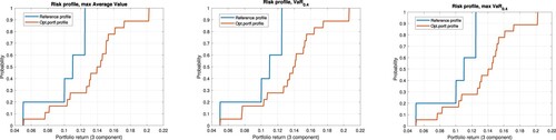
Figure 5. Profiles of optimal 3 component portfolios: maximizing the tail returns under the risk-return lower bound. Analytical projective penalties. (1) Optimal average return. (2) Optimal ${\mathrm{V}@\mathrm{R}}_{0.4}$. (3) Optimal ${\mathrm{AV}@\mathrm{R}}_{0.4}$. See Table 2.

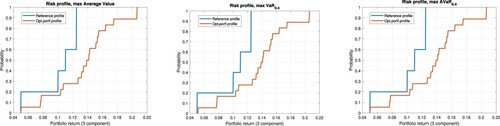
Table 1. Optimal 3 component portfolios, discontinuous penalties: (1) Max mean; (2) Max $\mathrm{V}@\mathrm{R}$; (3) Max $\mathrm{AV}@\mathrm{R}$.

Objective	Value	$x_4$	$x_9$	$x_{10}$
(1) Mean	0.1351	0.1229	0.0085	0.8675
(2) ${\mathrm{V}@\mathrm{R}}_{0.4}$	0.1344	0.1313	0.0001	0.8670
(3) ${\mathrm{AV}@\mathrm{R}}_{0.4}$	0.1554	0.1219	0.0105	0.8675

Note: See Figure 4.

Table 2. Optimal 3 component portfolios, analytical projection: (1) Max mean. (2) Max ${\mathrm{V}@\mathrm{R}}_{40\mathrm{\%}}$. (3) Max ${\mathrm{AV}@\mathrm{R}}_{40\mathrm{\%}}$.

Objective	Value	$x_4$	$x_9$	$x_{10}$
(1) Mean	0.1357	0.1308	0.0009	0.8683
(2) ${\mathrm{V}@\mathrm{R}}_{40\mathrm{\%}}$	0.1527	0.1298	0.0000	0.8702
(3) ${\mathrm{AV}@\mathrm{R}}_{40\mathrm{\%}}$	0.1709	0.1313	0.0004	0.8684

Note: See Figure 5.

The next two Tables 3 and 4 (and the corresponding Figures 6 and 7) show the effect of extension of a portfolio for account of new securities, from 3 to 10, for $\alpha =70\mathrm{\%}$. The objective functions values in Table 4 are greater than the corresponding values in Table 3. The corresponding Figures 6 and 7 indicate changes in the risk profiles of optimal portfolios due to this enlargement. The increase of the objective functions happens also for account of huddling the risk profiles to the reference ones. The pictures also show the influence of the different objective functions on the risk profiles of the optimal portfolios. Finally, Table 5 shows the structures of the optimal 10-component portfolios.

Figure 6. Profiles of optimal 3 component portfolios: maximizing the tail returns under the risk-return lower bound. Analytical projective penalties. (1) Optimal average return. (2) Optimal ${\mathrm{V}@\mathrm{R}}_{70\mathrm{\%}}$. (3) Optimal ${\mathrm{AV}@\mathrm{R}}_{70\mathrm{\%}}$. See Table 3.

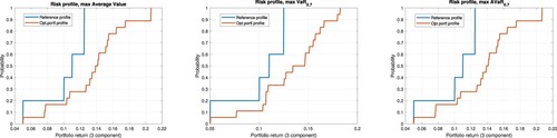
Figure 7. Profiles of optimal 10 component portfolios: maximizing the tail returns under the risk-return lower bound. Analytical projective penalties. (1) optimal average return; (2) optimal ${\mathrm{V}@\mathrm{R}}_{70\mathrm{\%}}$; (3) optimal ${\mathrm{AV}@\mathrm{R}}_{70\mathrm{\%}}$; cf. Tables 4 and 5.

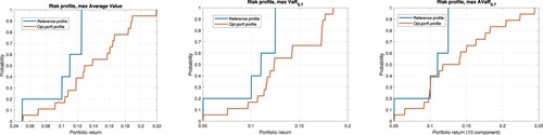
Table 3. Optimal 3 component portfolios, analytical projection: (1) Max mean. (2) Max $\mathrm{V}@\mathrm{R}$. (3) Max $\mathrm{AV}@\mathrm{R}$.

Objective	Value	$x_4$	$x_9$	$x_{10}$
(1) Mean	0.1357	0.1308	0.0009	0.8683
(2) ${\mathrm{V}@\mathrm{R}}_{70\mathrm{\%}}$	0.1549	0.0797	0.0557	0.8643
(3) ${\mathrm{AV}@\mathrm{R}}_{70\mathrm{\%}}$	0.1709	0.1315	0.0001	0.8684

Note: See Figure 6.

Table 4. Optimal 10 component portfolios, analytical projection: (1) Max mean. (2) Max $\mathrm{V}@\mathrm{R}$. (3) Max $\mathrm{AV}@\mathrm{R}$.

Objective	Value	$x_4$	$x_9$	$x_{10}$
(1) Mean	0.1380	0.0126	0.0022	0.8615
(2) ${\mathrm{V}@\mathrm{R}}_{70\mathrm{\%}}$	0.1728	0.0006	0.0425	0.8418
(3) ${\mathrm{AV}@\mathrm{R}}_{70\mathrm{\%}}$	0.1901	0.0126	0.0002	0.8490

Note: See Figure 7.

Table 5. The optimal 10 component portfolio.

Portfolio	$x_1$	$x_2$	$x_3$	$x_4$	$x_5$	$x_6$	$x_7$	$x_8$	$x_9$	$x_{10}$
Mean	.0013	.0001	.0059	.0126	.1011	.0008	.0031	.0117	.0022	.8615
${\mathrm{V}@\mathrm{R}}_{0.7}$	.0029	.0103	.0137	.0006	.0512	.0128	.0038	.0202	.0425	.8418
${\mathrm{AV}@\mathrm{R}}_{0.7}$	.0001	.0001	.0201	.0126	.0083	.0005	.0001	.1090	.0002	.8490

6.3. Summary of numerical experience

The concrete computational results of the numerical experiments depend on the following settings. We used

1. three different objective functions, the mean value, quantile and average quantile functions at different risk levels;

2. two kind of penalty functions, discontinuous and projective penalty ones (the latter is applied when there is an internal risk three portfolio);

3. a specific heuristic stochastic branch and bound algorithm with adjustable parameters;

4. several local optimization algorithms, Nemirovski-Yudin and Nesterov finite-difference stochastic optimization algorithms, and also a deterministic sequential quadratic programming one;

5. random starting points and adjustable parameters for local optimization algorithms.

The concrete computational results depend on all these options.

The problems under consideration can have many local optimums close to the global optimum, so the combined B&B algorithms may stick at different deep local optimums and may have different random running times (from several seconds to several minutes). To validate the global optimum, it is necessary to change the parameters of the algorithm and re-run it.

It was observed that the algorithm, combined algorithm with Nesterov's local optimization method, works better than combined with Nemirovski-Yudin's one. Besides, the combined heuristic B&B algorithm, which uses a well implemented deterministic sequential quadratic approximation algorithm (sqp from Matlab's optimization toolbox) as a local optimizer, works much faster (10 times or more) than stochastic optimization algorithms (seconds against minutes).

7. Conclusions

The paper considers a specific method for optimization, which transforms a constraint optimization problem to an unconstrained global optimization problem. The paper illustrates the procedure for an optimization problem with uncountable many constraints. More specifically, the paper considers financial portfolio optimization under 1-st order stochastic dominance constraints.

The designed optimization techniques are aimed at interactive solving the portfolio reshaping problem, i.e. interactive adaptation of the portfolio risk profile to the portfolio manager's preferences by changing risk bounds and optimization of different risk criteria.

In the literature, similar portfolio optimization problems are mostly considered under 2nd-order stochastic dominance constraints, which constitute convex problems. Few exceptions include [4,5,27,33,37,63]. The 1st-order constraints put lower bounds on the risk profile (CDF) of the optimized portfolio. As objective functions, different aggregated indicators can serve, e.g. the expected value, the Value-at-Risk, or the average Value-at-Risk, etc. In this setting, we put lower bounds on low returns and try to maximize higher returns.

Such constraints make the problem non-convex and hard for numerical treatment. We propose the new exact penalty functions to handle the constraints and a new stochastic B&B algorithm and new stochastic optimization (smoothing) techniques for solving penalty problems. The approach is numerically and graphically illustrated on small test examples. The advantage of the proposed approach to financial portfolio optimization consists in an additional visual control of the risk profile of the optimal portfolio.

The proposed B&B algorithm is well-suited for effective parallelization (parallel implementation of the B&B iteration) and thus has much room for acceleration and scaling and this may be a topic for future research.

Disclosure statement

This study builds upon publicly available data collected in Table 9. The corresponding data, codes, and tests are available at the first author's ResearchGate web-page. The authors have no conflicts of interest to disclose.

Additional information

Funding

Gratefully acknowledges funding by Volkswagenstiftung (Volkswagen Foundation) and National Research Fund of Ukraine – Project ID 2020.02/0121. DFG, German Research Foundation – Project-ID 416228727 – SFB 1410.

Appendix

Table A1. Return data set from [62, Table 1, page 13], with artificial bond column.

Year	Am.T.	A.T.&T.	U.S.S.	G.M.	A.T.&Sfe	C.C.	Bdn.	Frstn.	S.S.	Bond
1937	−0.305	−0.173	−0.318	−0.477	−0.457	−0.065	−0.319	−0.400	−0.435	0.125
1938	0.513	0.098	0.285	0.714	0.107	0.238	0.076	0.336	0.238	0.125
1939	0.055	0.200	−0.047	0.165	−0.424	−0.078	0.381	−0.093	−0.295	0.125
1940	−0.126	0.030	0.104	−0.043	−0.189	−0.077	−0.051	−0.090	−0.036	0.125
1941	−0.280	−0.183	−0.171	−0.277	0.637	−0.187	0.087	−0.400	−0.240	0.125
1942	−0.003	0.067	−0.039	0.476	0.865	0.156	0.262	1.113	0.126	0.125
1943	0.428	0.300	0.149	0.225	0.313	0.351	0.341	0.580	0.639	0.125
1944	0.192	0.103	0.260	0.290	0.637	0.233	0.227	0.473	0.282	0.125
1945	0.446	0.216	0.419	0.216	0.373	0.349	0.352	0.229	0.578	0.125
1946	−0.088	−0.046	−0.078	−0.272	−0.037	−0.209	0.153	−0.126	0.289	0.125
1947	−0.127	−0.071	0.169	0.144	0.026	0.355	−0.099	0.009	0.184	0.125
1948	−0.015	0.056	−0.035	0.107	0.153	−0.231	0.038	0.000	0.114	0.125
1949	0.305	0.038	0.133	0.321	0.067	0.246	0.273	0.223	−0.222	0.125
1950	−0.096	0.089	0.732	0.305	0.579	−0.248	0.091	0.650	0.327	0.125
1951	0.016	0.090	0.021	0.195	0.040	−0.064	0.054	−0.131	0.333	0.125
1952	0.128	0.083	0.131	0.390	0.434	0.079	0.109	0.175	0.062	0.125
1953	−0.010	0.035	0.006	−0.072	−0.027	0.067	0.210	−0.084	−0.048	0.125
1954	0.154	0.176	0.908	0.715	0.469	0.077	0.112	0.756	0.185	0.125

References

- Norkin VI. The projective exact penalty method for general constrained optimization. Preprint. V. M. Glushkov Institute of Cybernetics, Kyiv, 2022..
- Dentcheva D, Ruszczyński A. Optimization with stochastic dominance constraints. SIAM J Optim. 2003;14:548–566. doi: 10.1137/s1052623402420528
- Dentcheva D, Ruszczyński A. Portfolio optimization with stochastic dominance constraints. J Bank Financ. 2006;30:433–451. doi: 10.1016/j.jbankfin.2005.04.024
- Noyan N, Rudolf G, Ruszczyński A. Relaxations of linear programming problems with first order stochastic dominance constraints. Oper Res Lett. 2006;34:653–659. doi: 10.1016/j.orl.2005.10.004
- Noyan N, Ruszczyński A. Valid inequalities and restrictions for stochastic programming problems with first order stochastic dominance constraints. Math Program. 2008;114:249–275. doi: 10.1007/s10107-007-0100-1
- Shapiro A, Dentcheva D, Ruszczyński A. Lectures on stochastic programming. 3rd ed. SIAM; 2021. (MOS-SIAM Series on Optimization). doi: 10.1137/1.9781611976595
- Gutjahr WJ, Pichler A. Stochastic multi-objective optimization: a survey on non-scalarizing methods. Ann Oper Res. 2013;236(2):1–25. doi: 10.1007/s10479-013-1369-5
- Markowitz HM. Portfolio selection. J Finance. 1952;7(1):77–91. doi: 10.2307/2975974
- Roy AD. Safety first and the holding of assets. Econometrica. 1952;20:431–449. doi: 10.2307/1907413
- Artzner P, Delbaen F, Eber J-M, et al. Coherent measures of risk. Math Financ. 1999;9:203–228. doi: 10.1111/mafi.1999.9.issue-3
- Benati S, Rizzi R. A mixed integer linear programming formulation of the optimal mean/value-at-risk portfolio problem. Eur J Oper Res. 2007;176:423–434. doi: 10.1016/j.ejor.2005.07.020
- Gaivoronski AA, Pflug GC. Finding optimal portfolios with constraints on value-at-rrisk. In: Green B, editor, Proceedings of the Third International Stockholm Seminar on Risk Behaviour and Risk Management. Stockholm University; 1999.
- Gaivoronski AA, Pflug GC. Value at risk in portfolio optimization: properties and computational approach. J Risk. 2005;7:1–31. doi: 10.21314/JOR.2005.106
- Kataoka S. A stochastic programming model. Econometrica. 1963;31:181–196. doi: 10.2307/1910956
- Kibzun AI, Kan YS. Stochastic programming problems with probability and quantile functions. Chichester: John Wiley & Sons; 1996.
- Kibzun AI, Naumov AV, Norkin VI. On reducing a quantile optimization problem with discrete distribution to a mixed integer programming problem. Autom Remote Control. 2013;74:951–967. doi: 10.1134/S0005117913060064
- Kirilyuk V. Risk measures in stochastic programming and robust optimization problems. Cybern Syst Anal. 2015;51:874–885. doi: 10.1007/s10559-015-9780-3
- Luedtke J, Ahmed S, Nemhauser G. An integer programming approach for linear programs with probabilistic constraints. Math Program. 2010;122:247–272. doi: 10.1007/s10107-008-0247-4
- Norkin VI, Boyko SV. Safety-first portfolio selection. Cybern Syst Anal. 2012;48:180–191. doi: 10.1007/s10559-012-9396-9
- Norkin VI, Kibzun AI, Naumov AV. Reducing two-stage probabilistic optimization problems with discrete distribution of random data to mixed-integer programming problems. Cybern Syst Anal. 2014;50:679–692. doi: 10.1007/s10559-014-9658-9
- Pflug GC, Römisch W. Modeling, measuring and managing risk. River Edge (NJ): World Scientific; 2007. doi: 10.1142/9789812708724
- Prekopa A. Stochastic programming. Dordreht: Kluwer Academic Publisher; 1995.
- Sen S. Relaxation for probabilistically constrained programs with discrete random variables. Oper Res Lett. 1992;11:81–86. doi: 10.1016/0167-6377(92)90037-4
- Telser LG. Safety first and hedging. Rev Econ Stud. 1955/56;23:1–16. doi: 10.2307/2296146
- Wozabal D, Hochreiter R, Pflug GC. A D. C. formulation of value-at-risk constrained optimization. Optimization. 2010;59:377–400. doi: 10.1080/02331931003700731
- Rockafellar RT, Uryasev S. Optimization of conditional value-at-risk. J Risk. 2000;2(3):21–41. doi: 10.21314/JOR.2000.038
- Dentcheva D, Ruszczyński A. Risk preferences on the space of quantile functions. Math Program Ser B. 2013;148:181–200. doi: 10.1007/s10107-013-0724-2
- Müller A, Stoyan D. Comparison methods for stochastic models and risks. Chichester: John Wiley & Sons; 2002.
- Ogryczak W, Ruszczyński A. From stochastic dominance to mean-risk models: semideviations as risk measures. Eur J Oper Res. 1999;116:33–50. doi: 10.1016/S0377-2217(98)00167-2
- Ogryczak W, Ruszczyński A. On consistency of stochastic dominance and mean–semideviation models. Math Program Ser B. 2001;89:217–232. doi: 10.1007/s101070000203
- Ogryczak W, Ruszczyński A. Dual stochastic dominance and related mean-risk models. SIAM J Optim. 2002;13(1):60–78. doi: 10.1137/S1052623400375075
- Dentcheva D, Ruszczyński A. Common mathematical foundations of expected utility and dual utility theories. SIAM J Optim. 2013;23(1):381–405. doi: 10.1137/120868311
- Dai H, Xue Y, He N, et al. Learning to optimize with stochastic dominance constraints. In: International Conference on Artificial Intelligence and Statistics, PMLR; 2023; p. 8991–9009.
- Dentcheva D, Ruszczyński A. Portfolio optimization with risk control by stochastic dominance constraints. In: Infanger G., editor, Stochastic Programming. The State of the Art. In Honor of George B. Dantzig, chapter 9, pages 189–212. New York: Springer; 2011.
- Fábián CI, Mitra G, Roman D, et al. Portfolio choice models based on second-order stochastic dominance measures: An overview and a computational study. In M. Bertocchi, G. Consigli, and M. A. H. Dempster, editors, Stochastic optimization methods in finance and energy, International Series in Operations Research & Management Science, chapter 18, Springer: New York; 2011; p. 441–470. ISBN 978-1-4419-9586-5. doi: 10.1007/978-1-4419-9586-5_18
- Dentcheva D, Ruszczyński A. Risk preferences on the space of quantile functions. Math Program. 2014;148(1-2):181–200. doi: 10.1007/s10107-013-0724-2
- Dentcheva D, Ruszczyński A. Semi-infinite probabilistic optimization: first order stochastic dominance constraints. Optimization. 2004;53:583–601. doi: 10.1080/02331930412331327148
- Dentcheva D, Henrion R, Ruszczyński A. Stability and sensitivity of optimization problems with first order stochastic dominance constraints. SIAM J Optim. 2007;18:322–337. doi: 10.1137/060650118
- Frydenberg S, Sønsteng Henriksen TE, Pichler A, et al. Can commodities dominate stock and bond portfolios? Ann Oper Res. 2019;282(1-2):155–177. doi: 10.1007/s10479-018-2996-7
- Batukhtin V. On solving discontinuous extremal problems. J Optim Theory Appl. 1993;77:575–589. doi: 10.1007/BF00940451
- Knopov P, Norkin V. Stochastic optimization methods for the stochastic storage process control. M. J. Blondin et al. (eds.), Intelligent Control and Smart Energy Management, Springer Optimization and Its Applications 181, 2022; p. 79–111. doi: 10.1007/978-3-030-84474-5_3
- Norkin VI. A stochastic smoothing method for nonsmooth global optimization. Cybernetics and Computer technologies: 2020; p. 5–14. doi: 10.34229/2707-451X.20.1.1
- Ermoliev YM, Norkin VI, Wets RJ-B. The minimization of semicontinuous functions: mollifier subgradients. SIAM J Control Optim. 1995;33:149–167. doi: 10.1137/S0363012992238369
- Mayne D, Polak E. On solving discontinuous extremal problems. J Optim Theory Appl. 1984;43:601–613. doi: 10.1007/BF00935008
- Mikhalevich VS, Gupal AM, Norkin VI. Methods of nonconvex optimization. Moscow: Nauka; 1987. (In Russian).
- Nesterov Y, Spokoiny V. Random gradient-free minimization of convex functions. Found Comput Math. 2017;17:527–566. doi: 10.1007/s10208-015-9296-2
- Norkin V, Pflug GC, Ruszczyński A. A branch and bound method for stochastic global optimization. Math Program. 1998;83:425–450. doi: 10.1007/bf02680569
- Aubin J-P, Ekeland I. Applied nonlinear analysis. New York: John Wiley and Sons; 1984.
- Norkin VI. On measuring and profiling catastrophic risks. Cybern Syst Anal. 2006;42(6):839–850. doi: 10.1007/s10559-006-0124-1
- Galvan G, Sciandrone M, Eucidi S. A parameter-free unconstrained reformulation for nonsmooth problems with convex constraints. Comput Optim Appl. 2021;80:33–53. doi: 10.1007/s10589-021-00296-1
- Rockafellar RT, Wets RJ-B. Variational analysis. Grundlehren der mathematischen Wissenschaften. Springer, 1st ed. 1998, 3rd printing, springer edition, 2009. ISBN 3540627723; 9783540627722. doi: 10.1007/978-3-642-02431-3
- Ermoliev Y, Norkin V. On constrained discontinuous optimization. In: Stochastic Programming Methods and Technical Applications: Proceedings of the 3rd GAMM/IFIP-Workshop on ‘Stochastic Optimization: Numerical Methods and Technical Applications’ held at the Federal Armed Forces University Munich, Neubiberg/München, Germany, June 17–20, 1996, Springer: Berlin, Heidelberg; 1998; p. 128–144.
- Gupal AM, Norkin VI. Algorithm for the minimization of discontinuous functions. Cybernetics. 1977;13(2):220–223. doi: 10.1007/BF01073313
- Rockafellar RT, Wets RJ-B. Variational analysis. Switzerland AG: Springer Nature; 1997. Available at https://books.google.com/books?id=w-NdOE5fD8AC.doi: 10.1007/978-3-642-02431-3
- Norkin V, Pichler A, Kozyriev A. Constrained global optimization by smoothing. arXiv; 2023. doi: 10.48550/arXiv.2308.08422
- Nemirovsky A, Yudin D. Informational complexity and efficient methods for solution of convex extremal problems. New York: J. Wiley & Sons; 1983.
- Nesterov Y. A method of solving a convex programming problem with convergence rate. Soviet Math Dokl. 1983;27(2):372–376.
- Ermoliev YM. Methods of stochastic programming. Moscow: Nauka; 1976. (In Russian).
- Gupal AM. Stochastic methods for minimzation of nondifferentiable functions. Autom Remote Control. 1979;4(40):529–534.
- Polyak BT. Introduction to optimization. New York: Optimization Software, Inc. Publications Division; 1987.
- Pflug GC. Stepsize rules, stopping times, and their implementation in stochastic quasigradient algorithms. In: Ermoliev Y. and Wets RJ-B, editors, Numerical Techniques for Stochastic Optimization. Berlin: Springer-Verlag; 1988; chapter 17, p. 353–372.
- Markowitz HM. Portfolio selection. efficient diversification of investments. New York: John Wiley & Sons, Chapman & Hall; 1959.
- Luedtke J. New formulations for optimization under stochastic dominance constraints. SIAM J Optim. 2008;19(3):1433–1450. doi: 10.1137/070707956
Appendix
Table A1. Return data set from [Citation62, Table 1, page 13], with artificial bond column.