A fresh look at nonsmooth Levenberg–Marquardt methods with applications to bilevel optimization

Abstract

In this paper, we revisit the classical problem of solving over-determined systems of nonsmooth equations numerically. We suggest a nonsmooth Levenberg–Marquardt method for its solution which, in contrast to the existing literature, does not require local Lipschitzness of the data functions. This is possible when using Newton-differentiability instead of semismoothness as the underlying tool of generalized differentiation. Conditions for local fast convergence of the method are given. Afterwards, in the context of over-determined mixed nonlinear complementarity systems, our findings are applied, and globalized solution methods, based on a residual induced by the maximum and the Fischer–Burmeister function, respectively, are constructed. The assumptions for local fast convergence are worked out and compared. Finally, these methods are applied for the numerical solution of bilevel optimization problems. We recall the derivation of a stationarity condition taking the shape of an over-determined mixed nonlinear complementarity system involving a penalty parameter, formulate assumptions for local fast convergence of our solution methods explicitly, and present results of numerical experiments. Particularly, we investigate whether the treatment of the appearing penalty parameter as an additional variable is beneficial or not.

Keywords:

• Bilevel optimization
• mixed nonlinear complementarity problems
• Newton-differentiability
• nonsmooth Levenberg–Marquardt methods

Mathematics Subject Classifications:

• 49M05
• 49M15
• 90C30
• 90C33

1. Introduction

Nowadays, the numerical solution of nonsmooth equations is a classical topic in computational mathematics. Journeying 30 years back to the past, Qi and colleagues developed the celebrated nonsmooth Newton method, see [1, 2], based on the notion of semismoothness for locally Lipschitzian functions which is due to Mifflin, see [3]. Keeping the convincing local convergence properties of Newton-type methods in mind, this allowed for a fast numerical solution of Karush–Kuhn–Tucker systems, associated with constrained nonlinear optimization problems with inequality constraints, without the need of smoothing or relaxing the involved complementarity slackness condition. Indeed, the latter can be reformulated as a nonsmooth equation with the aid of so called NCP-functions, see [4–6] for an overview, where NCP abbreviates nonlinear complementarity problem. Recall that a continuous function $\phi :{\mathbb{R}}^2\to \mathbb{R}$ is referred to as an NCP-function whenever $\mathrm{\forall }(a,b)\in {\mathbb{R}}^2:\phi (a,b)=0⟺a\le 0,b\le 0,\mathrm{ab}=0$is valid. A rather prominent example of an NCP-function is the famous Fischer–Burmeister (FB) function ${\phi }_{\text{FB}}:{\mathbb{R}}^2\to \mathbb{R}$ given by (1) $\mathrm{\forall }(a,b)\in {\mathbb{R}}^2:{\phi }_{\text{FB}}(a,b):=a+b+\sqrt{a^2+b^2},$(1) see [7] for its origin. Another popular NCP-function is the maximum function $(a,b)\mapsto max(a,b)$. We refer the reader to [7–10] for further early references dealing with semismooth Newton-type methods to solve nonlinear complementarity systems. Let us note that even prior to the development of semismooth Newton methods 30 years ago, the numerical solution of nonsmooth equations via Newton-type algorithms has been addressed in the literature, see e.g. [11–15]. We refer the interested reader to the monographs [16–18] for a convincing overview.

Let us mention some popular directions of research which have been enriched or motivated by the theory of semismooth Newton methods. Exemplary, this theory has been extended to Levenberg–Marquardt (LM) methods in order to allow for the treatment of over-determined or irregular systems of equations, see e.g. [10, 19–22]. It also has been applied in order to solve so-called mixed nonlinear complementarity problems which are a natural extension of nonlinear complementarity problems and may also involve pure (smooth) equations, see e.g. [23–28]. Recently, the variational notion of semismoothness* for set-valued mappings has been introduced in [29] in order to discuss the convergence properties of Newton's method for the numerical solution of so-called generalized equations given via set-valued operators. There also exist infinite-dimensional extensions of nonsmooth Newton methods, see e.g. [30–36]. In contrast to the finite-dimensional case, in infinite dimensions, the underlying concept of semismoothness is often replaced by so-called Newton-differentiability. In principle, this notion of generalized differentiation encapsulates all necessities to address the convergence analysis of associated Newton-type methods properly. Noteworthy, it does not rely on the Lipschitzness of the underlying mapping. In the recent paper [37], this favourable advantage of Newton-derivatives has been used to construct a Newton-type method for the numerical solution of a certain stationarity system associated with so-called mathematical programs with complementarity constraints, as these stationarity conditions can be reformulated as a system of discontinuous equations.

Let us point the reader's attention to the fact that some stationarity conditions for bilevel optimization problems, see [38, 39] for an introduction, can be reformulated as (over-determined) systems of nonsmooth equations involving an (unknown) penalization parameter λ. This observation has been used in the recent papers [40–42] in order to solve bilevel optimization problems numerically. In [40], the authors used additional dummy variables in order to transform the naturally over-determined system into a square system, and applied a globalized semismooth Newton method for its computational solution. The papers [41, 42] directly tackle the over-determined nonsmooth system with Gauss–Newton or LM methods. However, in order to deal with the nonsmoothness, they either assume that strict complementarity holds or they smooth the complementarity condition. In all three papers [40–42], it has been pointed out that the choice of the penalty parameter λ in the stationarity system is, on the one hand, crucial for the success of the approach but, on the other hand, difficult to realize in practice.

The contributions in this paper touch several different aspects. Motivated by the results from [37], we study the numerical solution of over-determined systems of nonsmooth equations with the aid of LM methods based on the notion of Newton-differentiability. We show local superlinear convergence of this method under reasonable assumptions, see Theorem 3.2. Furthermore, we point out that even for local quadratic convergence, local Lipschitzness of the underlying mapping is not necessary. To be more precise, a one-sided Lipschitz estimate, which is referred to as calmness in the literature, is enough for that purpose. Thus, our theory applies to situations where the underlying mapping can be even discontinuous. Our next step is the application of this method for the numerical solution of over-determined mixed nonlinear complementarity systems. Here, we strike a classical path and reformulate the appearing complementarity conditions with the FB function and the maximum function in order to obtain a system of nonlinear equations. To globalize the associated Newton methods, we exploit the well-known fact that the squared norm of the residual associated with the FB function is continuously differentiable, and make use of gradient steps with respect to this squared norm in combination with an Armijo step size selection if LM directions do not yield sufficient improvements. We work out our abstract conditions guaranteeing local fast convergence for both approaches and state global convergence results in Theorems 4.6 and 4.12. Furthermore, we compare these findings with the ones in the classical paper [9] where a related comparison has been done in the context of semismooth Newton-type methods for square systems of nonsmooth equations. Finally, we apply both methods in order to solve bilevel optimization problems via their over-determined stationarity system of nonsmooth equations mentioned earlier. In contrast to [41, 42], we neither assume strict complementarity to hold nor do we smooth or relax the complementarity condition. Some assumptions for local fast convergence are worked out, see Theorems 5.3 and 5.4. As extensive numerical testing of related approaches has been carried out in [40–42], our experiments in Section 5.2 focus on specific features of the developed algorithms. Particularly, we comment on the possibility to treat the aforementioned penalty parameter λ as a variable, investigate this approach numerically, and compare the outcome with the situation where λ is handled as a parameter.

The remainder of the paper is organized as follows. Section 2 provides an overview of the notation and preliminaries used in the manuscript. Furthermore, we recall the notion of Newton-differentiability and present some associated calculus rules in Section 2.2. A local nonsmooth LM method for Newton-differentiable mappings is discussed in Section 3. Section 4 is dedicated to the derivation of globalized nonsmooth LM methods for the numerical solution of over-determined mixed nonlinear complementarity systems. First, we provide the analysis for the situation where the complementarity condition is reformulated with the maximum function in Section 4.1. Afterwards, in Section 4.2, we comment on the differences which pop up when the FB function is used instead. The obtained theory is used in Section 5 in order to solve bilevel optimization problems. In Section 5.1, we first recall the associated stationarity system of interest and characterize some scenarios where it provides necessary optimality conditions. Second, we present different ways on how to model these stationarity conditions as an over-determined mixed nonlinear complementarity system. The numerical solution of these systems with the aid of nonsmooth LM methods is then investigated in Section 5.2 where results of computational experiments are evaluated. The paper closes with some concluding remarks in Section 6.

2. Notation and preliminaries

2.1. Notation

By $\mathbb{N}$, we denote the positive integers. The set of all real matrices with $m\in \mathbb{N}$ rows and $n\in \mathbb{N}$ columns will be represented by ${\mathbb{R}}^{m\times n}$, and $\mathbb{O}$ denotes the all-zero matrix of appropriate dimensions while we use ${\mathbb{I}}^n$ for the identity matrix in ${\mathbb{R}}^{n\times n}$. If $M\in {\mathbb{R}}^{m\times n}$ is a matrix and $I\subset \{1,\dots ,m\}$ is arbitrary, then $M_I$ shall be the matrix which results from M by deleting those rows whose associated index does not belong to I. Whenever the quadratic matrix $N\in {\mathbb{R}}^{n\times n}$ is symmetric, ${\lambda }_{\text{min}}\left(N\right)$ denotes the smallest eigenvalue of N. For any $x\in {\mathbb{R}}^n$, $\mathrm{diag}\left(x\right)\in {\mathbb{R}}^{n\times n}$ is the diagonal matrix whose main diagonal is given by x and whose other entries vanish.

For arbitrary $n\in \mathbb{N}$, the space ${\mathbb{R}}^n$ will be equipped by the standard Euclidean inner product as well as the Euclidean norm $\Vert \cdot \Vert :{\mathbb{R}}^n\to \mathbb{R}$. Further, we equip ${\mathbb{R}}^{m\times n}$ with the matrix norm induced by the Euclidean norm, i.e. with the spectral norm, and denote it by $\Vert \cdot \Vert :{\mathbb{R}}^{m\times n}\to \mathbb{R}$ as well as this cannot cause any confusion. For arbitrary $x\in {\mathbb{R}}^n$ and $ϵ>0$, ${\mathbb{B}}_{ϵ}\left(x\right):=\{y\in {\mathbb{R}}^n|\Vert y-x\Vert \le ϵ\}$ represents the closed ε-ball around x. Recall that a sequence $\{x^k{\}}_{k\in \mathbb{N}}\subset {\mathbb{R}}^n$ is said to converge superlinearly to some $\overline{x}\in {\mathbb{R}}^n$ whenever $\Vert x^{k+1}-\overline{x}\Vert \in \mathcal{o}(\Vert x^k-\overline{x}\Vert )$. The convergence $x^k\to \overline{x}$ is said to be quadratic if $\Vert x^{k+1}-\overline{x}\Vert \in \mathcal{O}(\Vert x^k-\overline{x}{\Vert }^2)$.

Frequently, for brevity of notation, we interpret tuples of vectors as a single block column vector, i.e. we exploit the identity $\begin{array}{rl}& \mathrm{\forall i}\in \{1,\dots ,\ell \},\mathrm{\forall }{x}^i\in {\mathbb{R}}^{n_i}:\\ & {\mathbb{R}}^{n_1}\times \dots \times {\mathbb{R}}^{n_{\ell }}\ni (x^1,\dots ,x^{\ell })\cong \left[\begin{array}{c}{x}^1\\ ⋮\\ x^{\ell }\end{array}\right]\in {\mathbb{R}}^{n_1+\dots +n_{\ell }}\end{array}$for any $\ell \in \mathbb{N}$ with $\ell \ge 2$ and $n_1,\dots ,n_{\ell }\in \mathbb{N}$.

A function $H:{\mathbb{R}}^n\to {\mathbb{R}}^m$ is called calm at $\overline{x}\in {\mathbb{R}}^n$ whenever there are constants $C>0$ and $ϵ>0$ such that $\mathrm{\forall x}\in {\mathbb{B}}_{ϵ}\left(\overline{x}\right):\Vert H\left(x\right)-H\left(\overline{x}\right)\Vert \le C\Vert x-\overline{x}\Vert .$We note that calmness can be seen as a one-sided local Lipschitz property which is, in general, weaker than local Lipschitzness. Indeed, one can easily check that there exist functions which are calm at some fixed reference point but discontinuous in each neighbourhood of this point.

Next, let $H:{\mathbb{R}}^n\to {\mathbb{R}}^m$ be differentiable at $\overline{x}\in {\mathbb{R}}^n$. Then $H^{\prime }\left(\overline{x}\right)\in {\mathbb{R}}^{m\times n}$ denotes the Jacobian of H at $\overline{x}$. Similarly, for a differentiable scalar-valued function $h:{\mathbb{R}}^n\to \mathbb{R}$, $\mathrm{\nabla h}\left(\overline{x}\right)\in {\mathbb{R}}^n$ is the gradient of h at $\overline{x}$. Clearly, $h^{\prime }\left(\overline{x}\right)=\mathrm{\nabla h}(\overline{x}{)}^{\mathrm{\top }}$ by construction. In the case where h is twice differentiable, ${\mathrm{\nabla }}^{2}h\left(\overline{x}\right)\in {\mathbb{R}}^{n\times n}$ denotes the Hessian of h at $\overline{x}$. Partial derivatives with respect to particular variables are represented in analogous fashion.

We use $\mathrm{\Gamma }:{\mathbb{R}}^n\rightrightarrows {\mathbb{R}}^m$ is order to express that Γ is a so-called set-valued mapping which assigns to each $x\in {\mathbb{R}}^n$ a (potentially empty) subset of ${\mathbb{R}}^m$. For any such set-valued mapping, the sets defined by $\mathrm{dom}\mathrm{\Gamma }:=\{x\in {\mathbb{R}}^n|\mathrm{\Gamma }(x)\ne \mathrm{\varnothing }\}$ and $\mathrm{gph}\mathrm{\Gamma }:=\left\{\right(x,y)\in {\mathbb{R}}^n\times {\mathbb{R}}^m|y\in \mathrm{\Gamma }(x\left)\right\}$ are the domain and the graph of Γ, respectively. We say that Γ is inner semicontinuous at $(\overline{x},\overline{y})\in \mathrm{gph}\mathrm{\Gamma }$ whenever for each sequence $\{x^k{\}}_{k\in \mathbb{N}}\subset {\mathbb{R}}^n$ such that $x^k\to \overline{x}$, there exists a sequence $\{y^k{\}}_{k\in \mathbb{N}}\subset {\mathbb{R}}^m$ such that $y^k\to \overline{y}$ which satisfies $y^k\in \mathrm{\Gamma }\left(x^k\right)$ for all large enough $k\in \mathbb{N}$. We emphasize that whenever Γ is inner semicontinuous at $(\overline{x},\overline{y})$, then $\overline{x}$ is an interior point of $\mathrm{dom}\mathrm{\Gamma }$. At a fixed point $(\overline{x},\overline{y})\in \mathrm{gph}\mathrm{\Gamma }$, Γ is said to be calm whenever there are constants $ϵ,\delta ,L>0$ such that $\mathrm{\forall x}\in {\mathbb{B}}_{ϵ}\left(\overline{x}\right),\mathrm{\forall y}\in \mathrm{\Gamma }\left(x\right)\cap {\mathbb{B}}_{\delta }\left(\overline{y}\right),\mathrm{\exists }\tilde{y}\in \mathrm{\Gamma }\left(\overline{x}\right):\Vert y-\tilde{y}\Vert \le L\Vert x-\overline{x}\Vert .$We note that whenever $H:{\mathbb{R}}^n\to {\mathbb{R}}^m$ is a single-valued function which is calm at $\overline{x}$, then the set-valued mapping $x\mapsto \left\{H\right(x\left)\right\}$ is calm at $(\overline{x},H(\overline{x}\left)\right)$. The converse is not necessarily true.

2.2. Newton-differentiability

In order to construct numerical methods for the computational solution of nonsmooth equations, one has to choose a suitable concept of generalized differentiation. Typically, the idea of semismoothness is used for that purpose, see [2, 3]. Here, however, we strike a different path and exploit the notion of Newton-differentiability, see [32, 35], whose origins can be found in infinite-dimensional optimization. The latter has the inherent advantage that, in contrast to semismoothness, it is defined for non-Lipschitz functions and enjoys a natural calculus which follows the lines known from standard differentiability. These beneficial features have been used recently in order to solve stationarity conditions of complementarity-constrained optimization problems which can be reformulated as systems of discontinuous equations, see [37].

Let us start with the formal definition of Newton-differentiability before presenting some essential calculus rules. Most of this material is taken from the recent contribution [37, Section 2.3].

Definition 2.1

Let $\mathcal{F}:{\mathbb{R}}^p\to {\mathbb{R}}^q$ and $D_N\mathcal{F}:{\mathbb{R}}^p\to {\mathbb{R}}^{q\times p}$ be given mappings and let $M\subset {\mathbb{R}}^p$ be nonempty. We say that

1. $\mathcal{F}$ is Newton-differentiable on M with Newton-derivative $D_N\mathcal{F}$ whenever for each $z\in M$, we have $\mathcal{F}(z+d)-\mathcal{F}\left(z\right)-D_N\mathcal{F}(z+d)d=\mathcal{o}\left(\Vert d\Vert \right),$

2. $\mathcal{F}$ is Newton-differentiable on M of order $\alpha \in (0,1]$ with Newton-derivative $D_N\mathcal{F}$ whenever for each $z\in M$, we have $\mathcal{F}(z+d)-\mathcal{F}\left(z\right)-D_N\mathcal{F}(z+d)d=\mathcal{O}\left({\Vert d\Vert }^{1+\alpha }\right).$

We note that the Newton-derivative of a mapping $\mathcal{F}:{\mathbb{R}}^p\to {\mathbb{R}}^q$ is not necessarily uniquely determined if $\mathcal{F}$ is Newton-differentiable on some set $M\subset {\mathbb{R}}^p$. It can be easily checked that any continuously differentiable function $\mathcal{F}:{\mathbb{R}}^p\to {\mathbb{R}}^q$ is Newton-differentiable on ${\mathbb{R}}^p$ when $D_N\mathcal{F}:={\mathcal{F}}^{\prime }$ is chosen. If, additionally, ${\mathcal{F}}^{\prime }$ is locally Lipschitz continuous, then the order of Newton-differentiability is 1.

In the recent paper [37], the authors present several important calculus rules for Newton-derivatives including a chain rule which we recall below, see [37, Lemma 2.11].

Lemma 2.2

Suppose that $\mathcal{F}:{\mathbb{R}}^p\to {\mathbb{R}}^q$ is Newton-differentiable on $M\subset {\mathbb{R}}^p$ with Newton-derivative $D_N\mathcal{F}$, and that $\mathcal{G}:{\mathbb{R}}^q\to {\mathbb{R}}^s$ is Newton-differentiable on $\mathcal{F}\left(M\right)$ with Newton-derivative $D_N\mathcal{G}$. Further, assume that $D_N\mathcal{F}$ is bounded on a neighbourhood of M, and that $D_N\mathcal{G}$ is bounded on a neighbourhood of $\mathcal{F}\left(M\right)$. Then $\mathcal{G}\circ \mathcal{F}$ is Newton-differentiable on M with Newton-derivative given by $z\mapsto D_N\mathcal{G}\left(\mathcal{F}\right(z\left)\right)D_N\mathcal{F}\left(z\right)$. If both $\mathcal{F}$ and $\mathcal{G}$ are Newton-differentiable of order $\alpha \in (0,1]$, then $\mathcal{G}\circ \mathcal{F}$ is Newton-differentiable of order α with the Newton-derivative given above.

Let us note that Lemma 2.2 directly gives a sum rule which applies to the concept of Newton-differentiability. However, a direct proof via Definition 2.1 shows that a sum rule for Newton-differentiability holds without additional boundedness assumptions on the Newton-derivatives of the involved functions.

Let us inspect some examples which will be of major interest in this paper.

Example 2.3

1. The function $max:{\mathbb{R}}^2\to \mathbb{R}$ is Newton-differentiable on ${\mathbb{R}}^2$ of order 1 with Newton-derivative given by $\mathrm{\forall }(a,b)\in {\mathbb{R}}^2:D_{N}max(\cdot ,\cdot )(a,b):=\{\begin{array}{ll}(1,0)& a\ge b,\\ (0,1)& a<b,\end{array}$see [37, Example 2.8].

2. For arbitrary $p\in \mathbb{N}$, we investigate Newton-differentiability of the Euclidean norm $\Vert \cdot \Vert :{\mathbb{R}}^p\to \mathbb{R}$. Noting that $\Vert \cdot \Vert$ is continuously differentiable on ${\mathbb{R}}^p\setminus \left\{0\right\}$ with locally Lipschitzian derivative, it is Newton-differentiable of order 1 there. Let us consider the mapping $D_N\Vert \cdot \Vert :{\mathbb{R}}^p\to {\mathbb{R}}^{1\times p}$ given by (2) $\mathrm{\forall z}\in {\mathbb{R}}^p:D_N\Vert \cdot \Vert \left(z\right):=\{\begin{array}{ll}{\displaystyle \frac{z^{\mathrm{\top }}}{\Vert z\Vert }}& z\ne 0,\\ {\displaystyle \frac{\sqrt{p}}{p}{\mathtt{e}}^{\mathrm{\top }}}& z=0.\end{array}$(2) Here, $\mathtt{e}\in {\mathbb{R}}^p$ denotes the all-ones vector. At the origin, we have $\Vert d\Vert -D_N\Vert \cdot \Vert \left(d\right)d=0$ for each $d\in {\mathbb{R}}^p$, so we already obtain Newton-differentiability of $\Vert \cdot \Vert$ on ${\mathbb{R}}^p$ of order 1. We also note that the precise value of $D_N\Vert \cdot \Vert \left(0\right)$ is completely irrelevant for the validity of this property. However, the particular choice in (2(2) $\mathrm{\forall z}\in {\mathbb{R}}^p:D_N\Vert \cdot \Vert \left(z\right):=\{\begin{array}{ll}{\displaystyle \frac{z^{\mathrm{\top }}}{\Vert z\Vert }}& z\ne 0,\\ {\displaystyle \frac{\sqrt{p}}{p}{\mathtt{e}}^{\mathrm{\top }}}& z=0.\end{array}$(2) ) will be beneficial later on.

3. Let us investigate Newton-differentiability of the aforementioned FB function ${\phi }_{\text{FB}}:{\mathbb{R}}^2\to \mathbb{R}$ given in (1(1) $\mathrm{\forall }(a,b)\in {\mathbb{R}}^2:{\phi }_{\text{FB}}(a,b):=a+b+\sqrt{a^2+b^2},$(1) ). Relying on the sum rule (note that ${\phi }_{\text{FB}}$ is the sum of the identity and $\Vert \cdot \Vert$ in ${\mathbb{R}}^2$) and respecting our arguments from Example 2.3(b), we obtain that ${\phi }_{\text{FB}}$ is Newton-differentiable on ${\mathbb{R}}^2$ of order 1 with Newton-derivative given by $\begin{array}{r}{D}_N{\phi }_{\text{FB}}(a,b):=\{\begin{array}{ll}{\displaystyle (1+\frac{a}{\sqrt{a^2+b^2}},1+\frac{b}{\sqrt{a^2+b^2}})}& (a,b)\ne (0,0),\\ {\displaystyle (1+\frac{\sqrt{2}}{2},1+\frac{\sqrt{2}}{2})}& (a,b)=(0,0)\end{array}\end{array}$for all $(a,b)\in {\mathbb{R}}^2$, where we made use of (2(2) $\mathrm{\forall z}\in {\mathbb{R}}^p:D_N\Vert \cdot \Vert \left(z\right):=\{\begin{array}{ll}{\displaystyle \frac{z^{\mathrm{\top }}}{\Vert z\Vert }}& z\ne 0,\\ {\displaystyle \frac{\sqrt{p}}{p}{\mathtt{e}}^{\mathrm{\top }}}& z=0.\end{array}$(2) ).

3. A local nonsmooth Levenberg–Marquardt method

The paper [8] introduces a semismooth Newton-type method for square complementarity systems whose globalization is based on the FB function. An extension to LM-type methods (which even can handle inexact solutions of the subproblems) can be found in [10, 19]. A theoretical and numerical comparison of these methods is provided in [9]. An application of the semismooth LM method in the context of mixed complementarity systems can be found in [20], and these ideas were applied in the context of semiinfinite optimization e.g. in [21, 22].

In this subsection, we aim to analyse the local convergence properties of nonsmooth LM methods in a much broader context which covers not only the applications within the aforementioned papers, but also some new ones in bilevel optimization, see e.g. Section 5 and our comments in Section 6. Our approach via Newton-derivatives is slightly different from the one in the literature which exploits semismoothness of the underlying map of interest and, thus, particularly, local Lipschitz continuity.

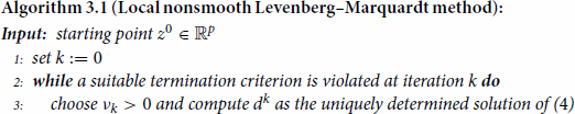
Throughout the subsection, we assume that $\mathcal{F}:{\mathbb{R}}^p\to {\mathbb{R}}^q$ is a given mapping with $q>p$ and inherent nonsmooth structure. We aim to solve the (over-determined) nonlinear system of equations (3) $\mathcal{F}\left(z\right)=0.$(3) Classically, this can be done by minimizing the squared residual of a first-order linearization associated with $\mathcal{F}$. The basic idea behind LM methods is now to add a classical square-norm regularization term to this optimization problem. Let us consider a current iterate $z^k$ where $\mathcal{F}$ is Newton-differentiable, and consider the minimization of $d\mapsto \frac{1}{2}{\Vert \mathcal{F}\left(z^k\right)+D_N\mathcal{F}\left(z^k\right)d\Vert }^2+\frac{{\nu }_k}{2}{\Vert d\Vert }^2$ which is a strictly convex function. Above, we exploited the Newton-derivative in order to find a linearization of $\mathcal{F}$ at $z^k$, and ${\nu }_k>0$ is a regularization parameter. By means of the chain rule, a necessary optimality condition for this surrogate problem is given by (4) $\left(D_N\mathcal{F}\right(z^k{)}^{\mathrm{\top }}{D}_N\mathcal{F}\left(z^k\right)+{\nu }_k{\mathbb{I}}^p)d=-D_N\mathcal{F}\left(z^k{)}^{\mathrm{\top }}\mathcal{F}\right(z^k).$(4) Observing that the matrix $D_N\mathcal{F}\left(z^k{)}^{\mathrm{\top }}{D}_N\mathcal{F}\right(z^k)$ is at least positive semidefinite, (4(4) $\left(D_N\mathcal{F}\right(z^k{)}^{\mathrm{\top }}{D}_N\mathcal{F}\left(z^k\right)+{\nu }_k{\mathbb{I}}^p)d=-D_N\mathcal{F}\left(z^k{)}^{\mathrm{\top }}\mathcal{F}\right(z^k).$(4) ) indeed possesses a uniquely determined solution $d^k$.

This motivates the formulation of Algorithm 3.1 for the numerical treatment of (3(3) $\mathcal{F}\left(z\right)=0.$(3) ). We assume that $D_N\mathcal{F}:{\mathbb{R}}^p\to {\mathbb{R}}^{q\times p}$ is a given function which serves as a Newton-derivative on a suitable subset of ${\mathbb{R}}^p$ which will be specified later.

In the subsequent theorem, we present a local convergence result regarding Algorithm 3.1.

Theorem 3.2

Let $M\subset {\mathbb{R}}^p$ be a set such that a solution $\overline{z}\in {\mathbb{R}}^p$ of (3(3) $\mathcal{F}\left(z\right)=0.$(3) ) satisfies $\overline{z}\in M$. Assume that $\mathcal{F}$ is Newton-differentiable on M with Newton-derivative $D_N\mathcal{F}:{\mathbb{R}}^p\to {\mathbb{R}}^{q\times p}$. We assume that there are $\delta >0$ and $C>0$ such that, for all $z\in {\mathbb{B}}_{\delta }\left(\overline{z}\right)$, $D_N\mathcal{F}\left(z\right)$ possesses full column rank p such that (5) ${\lambda }_{\text{min}}\left(D_N\mathcal{F}\right(z{)}^{\mathrm{\top }}{D}_N\mathcal{F}\left(z\right))\ge \frac{1}{C},\Vert D_N\mathcal{F}\left(z\right)\Vert \le C.$(5) Then there exists $ϵ>0$ such that, for each starting point $z^0\in {\mathbb{B}}_{ϵ}\left(\overline{z}\right)$ and each null sequence $\{{\nu }_k{\}}_{k\in \mathbb{N}}\subset (0,ϵ)$, Algorithm 3.1 terminates after finitely many steps or produces a sequence $\{z^k{\}}_{k\in \mathbb{N}}$ which converges to $\overline{z}$ superlinearly. Furthermore, if $\mathcal{F}$ is even Newton-differentiable on M of order 1, and if ${\nu }_k\in \mathcal{O}(\Vert \mathcal{F}(z^k)\Vert )$ while $\mathcal{F}$ is calm at $\overline{z}$, then the convergence is quadratic.

Proof.

Due to the assumptions of the theorem, and by Newton-differentiability of $\mathcal{F}$, we can choose $ϵ\in (0,min(\delta ,1/\left(4C\right))$ so small such that the following estimates hold true for all $d\in {\mathbb{B}}_{ϵ}\left(0\right)$ and $\nu >0$: (6a) $\begin{array}{rl}\Vert \left(D_N\mathcal{F}\right(\overline{z}+d{)}^{\mathrm{\top }}{D}_N\mathcal{F}(\overline{z}+d)+\nu {\mathbb{I}}^p{)}^{-1}\Vert & \le C,\end{array}$(6a) (6b) $\begin{array}{rl}\Vert D_N\mathcal{F}(\overline{z}+d)\Vert & \le C,\end{array}$(6b) (6c) $\begin{array}{rl}\Vert \mathcal{F}(\overline{z}+d)-\mathcal{F}\left(\overline{z}\right)-D_N\mathcal{F}(\overline{z}+d)d\Vert & \le \frac{1}{4C^2}\Vert d\Vert .\end{array}$(6c) Using $\mathcal{F}\left(\overline{z}\right)=0$, for each $z^k\in {\mathbb{B}}_{ϵ}\left(\overline{z}\right)$ and ${\nu }_k\in (0,ϵ)$, we find (7) $\begin{array}{rl}\Vert z^{k+1}-\overline{z}\Vert & =\Vert z^k-\left(D_N\mathcal{F}\right(z^k{)}^{\mathrm{\top }}{D}_N\mathcal{F}\left(z^k\right)+{\nu }_k{\mathbb{I}}^p{)}^{-1}{D}_N\mathcal{F}\left(z^k{)}^{\mathrm{\top }}\mathcal{F}\right(z^k)-\overline{z}\Vert \\ & \le C\Vert D_N\mathcal{F}\left(z^k{)}^{\mathrm{\top }}\right(\mathcal{F}\left(z^k\right)-\mathcal{F}\left(\overline{z}\right)-D_N\mathcal{F}\left(z^k\right)(z^k-\overline{z}))\Vert \\ & +C{\nu }_k\Vert z^k-\overline{z}\Vert \\ & \le C^2\Vert \mathcal{F}\left(z^k\right)-\mathcal{F}\left(\overline{z}\right)-D_N\mathcal{F}\left(z^k\right)(z^k-\overline{z})\Vert +C{\nu }_k\Vert z^k-\overline{z}\Vert \\ & \le \frac{1}{4}\Vert z^k-\overline{z}\Vert +\frac{1}{4}\Vert z^k-\overline{z}\Vert =\frac{1}{2}\Vert z^k-\overline{z}\Vert .\end{array}$(7) Thus, we have $\Vert z^{k+1}-\overline{z}\Vert \le \frac{1}{2}\Vert z^k-\overline{z}\Vert$, i.e. $z^{k+1}\in {\mathbb{B}}_{ϵ/2}\left(\overline{z}\right)$. Thus, if $z^0\in {\mathbb{B}}_{ϵ}\left(\overline{z}\right)$ and $\{{\nu }_k{\}}_{k\in \mathbb{N}}\subset (0,ϵ)$, we have $z^k\to \overline{z}$ in the case where Algorithm 3.1 generates an infinite sequence. Furthermore, the definition of Newton-differentiability, (7(7) $\begin{array}{rl}\Vert z^{k+1}-\overline{z}\Vert & =\Vert z^k-\left(D_N\mathcal{F}\right(z^k{)}^{\mathrm{\top }}{D}_N\mathcal{F}\left(z^k\right)+{\nu }_k{\mathbb{I}}^p{)}^{-1}{D}_N\mathcal{F}\left(z^k{)}^{\mathrm{\top }}\mathcal{F}\right(z^k)-\overline{z}\Vert \\ & \le C\Vert D_N\mathcal{F}\left(z^k{)}^{\mathrm{\top }}\right(\mathcal{F}\left(z^k\right)-\mathcal{F}\left(\overline{z}\right)-D_N\mathcal{F}\left(z^k\right)(z^k-\overline{z}))\Vert \\ & +C{\nu }_k\Vert z^k-\overline{z}\Vert \\ & \le C^2\Vert \mathcal{F}\left(z^k\right)-\mathcal{F}\left(\overline{z}\right)-D_N\mathcal{F}\left(z^k\right)(z^k-\overline{z})\Vert +C{\nu }_k\Vert z^k-\overline{z}\Vert \\ & \le \frac{1}{4}\Vert z^k-\overline{z}\Vert +\frac{1}{4}\Vert z^k-\overline{z}\Vert =\frac{1}{2}\Vert z^k-\overline{z}\Vert .\end{array}$(7) ), and ${\nu }_k\to 0$ give $\Vert z^{k+1}-\overline{z}\Vert =\mathcal{o}(\Vert z^k-\overline{z}\Vert )$, i.e. the convergence $z^k\to \overline{z}$ is superlinear.

Finally, assume that $\mathcal{F}$ is Newton-differentiable of order 1 and calm at $\overline{z}$, and that ${\nu }_k\in \mathcal{O}(\Vert \mathcal{F}(z^k)\Vert )$. Then there is a constant $K>0$ such that the estimate (7(7) $\begin{array}{rl}\Vert z^{k+1}-\overline{z}\Vert & =\Vert z^k-\left(D_N\mathcal{F}\right(z^k{)}^{\mathrm{\top }}{D}_N\mathcal{F}\left(z^k\right)+{\nu }_k{\mathbb{I}}^p{)}^{-1}{D}_N\mathcal{F}\left(z^k{)}^{\mathrm{\top }}\mathcal{F}\right(z^k)-\overline{z}\Vert \\ & \le C\Vert D_N\mathcal{F}\left(z^k{)}^{\mathrm{\top }}\right(\mathcal{F}\left(z^k\right)-\mathcal{F}\left(\overline{z}\right)-D_N\mathcal{F}\left(z^k\right)(z^k-\overline{z}))\Vert \\ & +C{\nu }_k\Vert z^k-\overline{z}\Vert \\ & \le C^2\Vert \mathcal{F}\left(z^k\right)-\mathcal{F}\left(\overline{z}\right)-D_N\mathcal{F}\left(z^k\right)(z^k-\overline{z})\Vert +C{\nu }_k\Vert z^k-\overline{z}\Vert \\ & \le \frac{1}{4}\Vert z^k-\overline{z}\Vert +\frac{1}{4}\Vert z^k-\overline{z}\Vert =\frac{1}{2}\Vert z^k-\overline{z}\Vert .\end{array}$(7) ) can be refined as $\begin{array}{rl}\Vert z^{k+1}-\overline{z}\Vert & \le C^2\Vert \mathcal{F}\left(z^k\right)-\mathcal{F}\left(\overline{z}\right)-D_N\mathcal{F}\left(z^k\right)(z^k-\overline{z})\Vert +C{\nu }_k\Vert z^k-\overline{z}\Vert \\ & \le \mathcal{O}(\Vert z^k-\overline{z}{\Vert }^2)+\mathrm{CK}\Vert \mathcal{F}\left(z^k\right)\Vert \Vert z^k-\overline{z}\Vert \\ & =\mathcal{O}(\Vert z^k-\overline{z}{\Vert }^2),\end{array}$where we used $\mathcal{F}\left(\overline{z}\right)=0$ and the calmness of $\mathcal{F}$ at $\overline{z}$ in the last step.

Let us briefly compare the assumptions of Theorem 3.2, which are used to guarantee the superlinear or quadratic convergence of a sequence generated by Algorithm 3.1, with the ones exploited in the literature where nonsmooth LM methods are considered from the viewpoint of semismoothness, see e.g. [10, Section 2]. Therefore, we fix a solution $\overline{z}\in {\mathbb{R}}^p$ of (3(3) $\mathcal{F}\left(z\right)=0.$(3) ). The full column rank assumption on the Newton-derivative, locally around $\overline{z}$, corresponds to so-called BD-regularity of the point $\overline{z}$ which demands that all matrices within Bouligand's generalized Jacobian at $\overline{z}$ (if available), see e.g. [1, Section 2], possess full column rank. We note that, by upper semicontinuity of Bouligand's generalized Jacobian, this full rank assumption extends to a neighbourhood of $\overline{z}$. Hence, these full rank assumptions are, essentially, of the same type although the one from Theorem 3.2 is more general since it addresses situations where the underlying map is allowed to be non-Lipschitz. Second, Theorem 3.2 assumes boundedness of the Newton-derivative, locally around $\overline{z}$. In the context of semismooth LM methods, local boundedness of the generalized derivative holds inherently by construction of Bouligand's generalized Jacobian and local Lipschitzness of the underlying mapping. Third, for quadratic convergence, the regularization parameters need to satisfy ${\nu }_k\in \mathcal{O}(\Vert \mathcal{F}(z^k)\Vert )$ in Theorem 3.2, and this assumption is also used in [10]. Similarly, since Newton-differentiability of order 1 is a natural counterpart of so-called strict semismoothness, the assumptions for quadratic convergence are also the same. Summarizing these impressions, Algorithm 3.1 and Theorem 3.2 generalize the already existing theory on nonsmooth LM methods to a broader setting under reasonable assumptions. We also note that our analysis made no use of deeper underlying properties of the generalized derivative, we mainly used its definition for our purposes. However, it should be observed that a sophisticated choice of the Newton-derivative, which is not uniquely determined for a given map as mentioned in Section 2.2, may lead to weaker assumptions in Theorem 3.2 than a bad choice of it. Indeed, it even may happen that the assumptions of Theorem 3.2 are valid for a particular choice of the Newton-derivative while they are violated for another one. Thus, when Algorithm 3.1 (or a suitable globalization) is implemented, one has to keep in mind to choose the Newton-derivative in such a way that the assumptions of Theorem 3.2 are valid (if this is actually possible), as the requirements of Theorem 3.2 need to be satisfied for one particular choice of the Newton-derivative (and not for all possible choices). Clearly, this choice depends on structural properties of the nonsmooth mapping $\mathcal{F}$ under consideration and is, potentially, a laborious task as we will see in Section 4, see [37] as well.

The following corollary of Theorem 3.2 shows that $\Vert \mathcal{F}\left(z^{k+1}\right)\Vert \in \mathcal{o}(\Vert \mathcal{F}(z^k)\Vert )$ can be expected under reasonable assumptions, and this will be of essential importance later on.

Corollary 3.3

Under the assumptions of Theorem 3.2 which guarantee the superlinear convergence of $\{z^k{\}}_{k\in \mathbb{N}}$ generated by Algorithm 3.1, we additionally have $\frac{\Vert \mathcal{F}\left(z^{k+1}\right)\Vert }{\Vert \mathcal{F}\left(z^k\right)\Vert }\to 0$provided $\mathcal{F}$ is calm at $\overline{z}$.

Proof.

We choose $ϵ>0$ as in the proof of Theorem 3.2 and observe $\{z^k{\}}_{k\in \mathbb{N}}\subset {\mathbb{B}}_{ϵ}(\overline{z})$. Exploiting the Newton-differentiability of $\mathcal{F}$ and $\mathcal{F}\left(\overline{z}\right)=0$, we have $\mathcal{F}\left(z^k\right)=D_N\mathcal{F}\left(z^k\right)(z^k-\overline{z})+\mathcal{o}(\Vert z^k-\overline{z}\Vert ),$and some transformations give, for sufficiently large $k\in \mathbb{N}$ and by boundedness of the sequence $\left\{D_N\mathcal{F}\right(z^k){\}}_{k\in \mathbb{N}}$, $\Vert z^k-\overline{z}\Vert \le \Vert \left(D_N\mathcal{F}\right(z^k{)}^{\mathrm{\top }}{D}_N\mathcal{F}\left(z^k\right){)}^{-1}{D}_N\mathcal{F}\left(z^k{)}^{\mathrm{\top }}\mathcal{F}\right(z^k)\Vert +\frac{1}{2}\Vert z^k-\overline{z}\Vert ,$i.e. $\frac{1}{2}\Vert z^k-\overline{z}\Vert \le \Vert \left(D_N\mathcal{F}\right(z^k{)}^{\mathrm{\top }}{D}_N\mathcal{F}\left(z^k\right){)}^{-1}\Vert \Vert D_N\mathcal{F}\left(z^k\right)\Vert \Vert \mathcal{F}\left(z^k\right)\Vert \le C^2\Vert \mathcal{F}\left(z^k\right)\Vert$due to (5(5) ${\lambda }_{\text{min}}\left(D_N\mathcal{F}\right(z{)}^{\mathrm{\top }}{D}_N\mathcal{F}\left(z\right))\ge \frac{1}{C},\Vert D_N\mathcal{F}\left(z\right)\Vert \le C.$(5) ). Thus, we find $\begin{array}{rl}\frac{\Vert \mathcal{F}\left(z^{k+1}\right)\Vert }{\Vert \mathcal{F}\left(z^k\right)\Vert }& \le \frac{2C^2\Vert \mathcal{F}\left(z^{k+1}\right)-\mathcal{F}\left(\overline{z}\right)\Vert }{\Vert z^k-\overline{z}\Vert }\le \frac{2C^{2}L\Vert z^{k+1}-\overline{z}\Vert }{\Vert z^k-\overline{z}\Vert }\\ & \le \frac{2C^{2}L\mathcal{o}(\Vert z^k-\overline{z}\Vert )}{\Vert z^k-\overline{z}\Vert }\to 0\end{array}$as $k\to \mathrm{\infty }$, where $L>0$ is a local calmness constant of $\mathcal{F}$ at $\overline{z}$.

In [37, Section 3.2], a function is constructed which possesses the following properties:

1. it is Newton-differentiable on its set of roots with globally bounded and nonvanishing Newton-derivative,

2. it is discontinuous in each open neighbourhood of its set of roots, and

3. it is calm at each point from its set of roots.

This function is then used to construct a nonsmooth Newton-type method for the computational solution of stationarity systems associated with complementarity-constrained optimization problems. We note that it crucially violates the standard requirement of local Lipschitzness which is typically exploited in the context of nonsmooth Newton-type methods. Similarly as in [37], the analysis in Theorem 3.2 and Corollary 3.3 only requires calmness of the mapping $\mathcal{F}$ (as well as some other natural assumptions) in order to get local fast convergence of a nonsmooth LM method. Thus, the ideas from [37] can be carried over to the situation where over-determined stationarity systems of complementarity-constrained optimization problems need to be solved (such systems would, exemplary, arise when applying the theory from Section 5.1 to bilevel optimization problems with additional complementarity constraints at the upper-level stage or to the so-called combined reformulation of bilevel optimization problems which makes use of the so-called value function and Karush–Kuhn–Tucker reformulation at the same time, see [43]).

For the globalization of Algorithm 3.1, one typically needs to impose additional assumptions like the smoothness of $z\mapsto {\Vert \mathcal{F}\left(z\right)\Vert }^2$. In the next section, we address the prototypical setting of mixed nonlinear complementarity systems and carve out two classical globalization strategies.

4. A global nonsmooth Levenberg–Marquardt method for mixed nonlinear complementarity systems

For functions $\mathcal{H}:{\mathbb{R}}^{p_1}\times {\mathbb{R}}^{p_2}\to {\mathbb{R}}^{q_1}$ and $\mathcal{G}:{\mathbb{R}}^{p_1}\times {\mathbb{R}}^{p_2}\to {\mathbb{R}}^{p_2}$ being continuously differentiable, we aim to solve the mixed nonlinear complementarity system (MNLCS) $\mathcal{H}(w,\xi )=0,\mathcal{G}(w,\xi )\le 0,\xi \ge 0,\mathcal{G}(w,\xi {)}^{\mathrm{\top }}\xi =0$(MNLCS) where, in the application we have in mind, $q_1>p_1$ holds true, see Section 5. A comprehensive overview of available theoretical and numerical aspects as well as applications of mixed nonlinear complementarity problems can be found in the monograph [16]. Typical solution approaches are based on nonsmooth Newton-type methods, see [26], smoothing methods, see [23, 27], active-set and interior-point methods, see [24, 28], as well as penalty methods, see [25]. Let us note that the classical formulation of mixed nonlinear complementarity systems as considered in [23, 24, 26–28] is essentially equivalent to the one we are suggesting in (MNLCS(MNLCS) $\mathcal{H}(w,\xi )=0,\mathcal{G}(w,\xi )\le 0,\xi \ge 0,\mathcal{G}(w,\xi {)}^{\mathrm{\top }}\xi =0$(MNLCS) ), see [23, Section 4] and [24, Section 1] for arguments which reveal this equivalence. However, in Section 5, it will be beneficial to work with the model (MNLCS(MNLCS) $\mathcal{H}(w,\xi )=0,\mathcal{G}(w,\xi )\le 0,\xi \ge 0,\mathcal{G}(w,\xi {)}^{\mathrm{\top }}\xi =0$(MNLCS) ) to preserve structural properties.

For later use, we introduce some index sets depending on a pair of vectors $(w,\xi )\in {\mathbb{R}}^{p_1}\times {\mathbb{R}}^{p_2}$: $\begin{array}{rl}{I}^0(w,\xi )& :=\{i\in \{1,\dots ,p_2\left\}|{\mathcal{G}}_i\right(w,\xi )=0\},\\ I^{-}(w,\xi )& :=\{i\in \{1,\dots ,p_2\left\}|{\mathcal{G}}_i\right(w,\xi \left)<0\right\},\\ I^{+}(w,\xi )& :=\{i\in I^0(w,\xi \left)|{\xi }_i>0\right\},\\ I^{00}(w,\xi )& :=\{i\in I^0(w,\xi )|{\xi }_i=0\}.\end{array}$Above, ${\mathcal{G}}_1,\dots ,{\mathcal{G}}_{p_2}:{\mathbb{R}}^{p_1}\times {\mathbb{R}}^{p_2}\to \mathbb{R}$ are the component functions of $\mathcal{G}$.

Based on NCP-functions, see Section 1, the complementarity condition (8) $\mathcal{G}(w,\xi )\le 0,\xi \ge 0,\mathcal{G}(w,\xi {)}^{\mathrm{\top }}\xi =0$(8) can be restated in form of a (nonsmooth) equality constraint. In this paper, we will focus on two popular choices, namely the maximum function and the famous FB function. Clearly, (8(8) $\mathcal{G}(w,\xi )\le 0,\xi \ge 0,\mathcal{G}(w,\xi {)}^{\mathrm{\top }}\xi =0$(8) ) is equivalent to $max\left(\mathcal{G}\right(w,\xi ),-\xi )=0,$where $max:{\mathbb{R}}^{p_2}\times {\mathbb{R}}^{p_2}\to {\mathbb{R}}^{p_2}$ is exploited to express the componentwise maximum. Using ${\varphi }_{\text{FB}}:{\mathbb{R}}^{p_2}\times {\mathbb{R}}^{p_2}\to {\mathbb{R}}^{p_2}$, given by $\mathrm{\forall }{\xi }^1,{\xi }^2\in {\mathbb{R}}^{p_2}:{\varphi }_{\text{FB}}({\xi }^1,{\xi }^2):=\left(\begin{array}{c}{\phi }_{\text{FB}}({\xi }_1^1,{\xi }_1^2)\\ ⋮\\ {\phi }_{\text{FB}}({\xi }_{p_2}^1,{\xi }_{p_2}^2)\end{array}\right),$where ${\phi }_{\text{FB}}:{\mathbb{R}}^2\to \mathbb{R}$ is the FB function defined in (1(1) $\mathrm{\forall }(a,b)\in {\mathbb{R}}^2:{\phi }_{\text{FB}}(a,b):=a+b+\sqrt{a^2+b^2},$(1) ), (8(8) $\mathcal{G}(w,\xi )\le 0,\xi \ge 0,\mathcal{G}(w,\xi {)}^{\mathrm{\top }}\xi =0$(8) ) is also equivalent to ${\varphi }_{\text{FB}}\left(\mathcal{G}\right(w,\xi ),-\xi )=0.$These nonsmooth equations motivate the consideration of the special residual mappings ${\mathcal{F}}_{\text{max}},{\mathcal{F}}_{\text{FB}}:{\mathbb{R}}^{p_1}\times {\mathbb{R}}^{p_2}\to {\mathbb{R}}^{q_1}\times {\mathbb{R}}^{p_2}$ given by (9) $\begin{array}{rl}\mathrm{\forall w}\in {\mathbb{R}}^{p_1},\mathrm{\forall \xi }\in {\mathbb{R}}^{p_2}:{\mathcal{F}}_{\text{max}}(w,\xi )& :=\left[\begin{array}{c}\mathcal{H}(w,\xi )\\ max\left(\mathcal{G}\right(w,\xi ),-\xi )\end{array}\right],\\ {\mathcal{F}}_{\text{FB}}(w,\xi )& :=\left[\begin{array}{c}\mathcal{H}(w,\xi )\\ {\varphi }_{\text{FB}}\left(\mathcal{G}\right(w,\xi ),-\xi )\end{array}\right],\end{array}$(9) since precisely their roots are the solutions of (MNLCS(MNLCS) $\mathcal{H}(w,\xi )=0,\mathcal{G}(w,\xi )\le 0,\xi \ge 0,\mathcal{G}(w,\xi {)}^{\mathrm{\top }}\xi =0$(MNLCS) ). Let us note that, in a certain sense, these residuals are equivalent. This can be distilled from [44, Lemma 3.1].

Lemma 4.1

There exist constants $K_1,K_2>0$ such that $\mathrm{\forall w}\in {\mathbb{R}}^{p_1},\mathrm{\forall \xi }\in {\mathbb{R}}^{p_2}:K_1\Vert {\mathcal{F}}_{\text{max}}(w,\xi )\Vert \le \Vert {\mathcal{F}}_{\text{FB}}(w,\xi )\Vert \le K_2\Vert {\mathcal{F}}_{\text{max}}(w,\xi )\Vert .$

Due to the inherent nonsmoothness of ${\mathcal{F}}_{\text{max}}$ and ${\mathcal{F}}_{\text{FB}}$ from (9(9) $\begin{array}{rl}\mathrm{\forall w}\in {\mathbb{R}}^{p_1},\mathrm{\forall \xi }\in {\mathbb{R}}^{p_2}:{\mathcal{F}}_{\text{max}}(w,\xi )& :=\left[\begin{array}{c}\mathcal{H}(w,\xi )\\ max\left(\mathcal{G}\right(w,\xi ),-\xi )\end{array}\right],\\ {\mathcal{F}}_{\text{FB}}(w,\xi )& :=\left[\begin{array}{c}\mathcal{H}(w,\xi )\\ {\varphi }_{\text{FB}}\left(\mathcal{G}\right(w,\xi ),-\xi )\end{array}\right],\end{array}$(9) ), we may now apply Algorithm 3.1 in order to solve ${\mathcal{F}}_{\text{max}}(w,\xi )=0$ or ${\mathcal{F}}_{\text{FB}}(w,\xi )=0$. Note that we have $p:=p_1+p_2$ and $q:=q_1+p_2$ in the context of Section 3. In the literature, the approach via ${\mathcal{F}}_{\text{FB}}$ is quite popular due to the well-known observation that the mapping ${\mathrm{\Psi }}_{\text{FB}}:{\mathbb{R}}^{p_1}\times {\mathbb{R}}^{p_2}\to \mathbb{R}$ given by $\mathrm{\forall w}\in {\mathbb{R}}^{p_1},\mathrm{\forall \xi }\in {\mathbb{R}}^{p_2}:{\mathrm{\Psi }}_{\text{FB}}(w,\xi ):=\frac{1}{2}\Vert {\mathcal{F}}_{\text{FB}}(w,\xi ){\Vert }^2$is continuously differentiable, allowing for a globalization of suitable local solution methods. This is due to the fact that the squared FB function is continuously differentiable, see e.g. [45, Lemma 3.4]. However, it has been reported in [9] in the context of square nonlinear complementarity systems that a mixed approach combining both residuals from (9(9) $\begin{array}{rl}\mathrm{\forall w}\in {\mathbb{R}}^{p_1},\mathrm{\forall \xi }\in {\mathbb{R}}^{p_2}:{\mathcal{F}}_{\text{max}}(w,\xi )& :=\left[\begin{array}{c}\mathcal{H}(w,\xi )\\ max\left(\mathcal{G}\right(w,\xi ),-\xi )\end{array}\right],\\ {\mathcal{F}}_{\text{FB}}(w,\xi )& :=\left[\begin{array}{c}\mathcal{H}(w,\xi )\\ {\varphi }_{\text{FB}}\left(\mathcal{G}\right(w,\xi ),-\xi )\end{array}\right],\end{array}$(9) ) might be beneficial since the assumptions for local fast convergence could be weaker while the local convergence is faster.

4.1. The mixed approach via both residual functions

First, let us focus on this mixed approach where the central LM search direction will be computed via ${\mathcal{F}}_{\text{max}}$ given in (9(9) $\begin{array}{rl}\mathrm{\forall w}\in {\mathbb{R}}^{p_1},\mathrm{\forall \xi }\in {\mathbb{R}}^{p_2}:{\mathcal{F}}_{\text{max}}(w,\xi )& :=\left[\begin{array}{c}\mathcal{H}(w,\xi )\\ max\left(\mathcal{G}\right(w,\xi ),-\xi )\end{array}\right],\\ {\mathcal{F}}_{\text{FB}}(w,\xi )& :=\left[\begin{array}{c}\mathcal{H}(w,\xi )\\ {\varphi }_{\text{FB}}\left(\mathcal{G}\right(w,\xi ),-\xi )\end{array}\right],\end{array}$(9) ) in order to end up with less complicated Newton-derivatives in the LM system. Still, we exploit the smooth function ${\mathrm{\Psi }}_{\text{FB}}$ for globalization purposes. Later, in Section 4.2, we briefly comment on the method which exclusively uses ${\mathcal{F}}_{\text{FB}}$.

Below, we provide formulas for a Newton-derivative of ${\mathcal{F}}_{\text{max}}$ and the gradient of ${\mathrm{\Psi }}_{\text{FB}}$ for later use.

Lemma 4.2

On each bounded subset of ${\mathbb{R}}^{p_1}\times {\mathbb{R}}^{p_2}$, the mapping ${\mathcal{F}}_{\text{max}}$ is Newton-differentiable with Newton-derivative given by $(w,\xi )\mapsto \left[\begin{array}{cc}{\mathcal{H}}_w^{\prime }(w,\xi )& {\mathcal{H}}_{\xi }^{\prime }(w,\xi )\\ \mathbb{D}\left(I^{\ge }\right(w,\xi \left)\right){\mathcal{G}}_w^{\prime }(w,\xi )& \mathbb{D}\left(I^{\ge }\right(w,\xi \left)\right){\mathcal{G}}_{\xi }^{\prime }(w,\xi )-\mathbb{D}\left(I^{<}\right(w,\xi \left)\right)\end{array}\right],$and this mapping, again, is bounded on bounded sets. Whenever the derivatives of $\mathcal{G}$ and $\mathcal{H}$ are locally Lipschitzian, the order of Newton-differentiability is 1. Above, the index sets $I^{\ge }(w,\xi )$ and $I^{<}(w,\xi )$ are given by $\begin{array}{rl}{I}^{\ge }(w,\xi )& :=\{i\in \{1,\dots ,p_2\left\}|{\mathcal{G}}_i\right(w,\xi )\ge -{\xi }_i\},\\ I^{<}(w,\xi )& :=\{i\in \{1,\dots ,p_2\left\}|{\mathcal{G}}_i\right(w,\xi )<-{\xi }_i\},\end{array}$and, for each $I\subset \{1,\dots ,p_2\}$, $\mathbb{D}\left(I\right)\in {\mathbb{R}}^{p_2\times p_2}$ is the diagonal matrix given by $\mathrm{\forall i},j\in \{1,\dots ,p_2\}:\mathbb{D}(I{)}_{\mathrm{ij}}:=\{\begin{array}{ll}1& i=j,i\in I,\\ 0& \text{otherwise.}\end{array}$

Proof.

This follows easily from Lemma 2.2, Example 2.3(a), and our comments right after Definition 2.1.

Throughout the section, we will denote the Newton-derivative of ${\mathcal{F}}_{\text{max}}$ which has been characterized in Lemma 4.2 by $D_N{\mathcal{F}}_{\text{max}}$.

The next result follows simply by computing the derivative of the squared FB function and using the standard chain rule.

Lemma 4.3

At each point $(w,\xi )\in {\mathbb{R}}^{p_1}\times {\mathbb{R}}^{p_2}$, ${\mathrm{\Psi }}_{\text{FB}}$ is continuously differentiable, and its gradient is given by $\begin{array}{rl}& \mathrm{\nabla }{\mathrm{\Psi }}_{\text{FB}}(w,\xi )\\ & ={\left[\begin{array}{cc}{\mathcal{H}}_w^{\prime }(w,\xi )& {\mathcal{H}}_{\xi }^{\prime }(w,\xi )\\ {\tilde{\mathbb{D}}}_{\mathcal{G}}(w,\xi ){\mathcal{G}}_w^{\prime }(w,\xi )& {\tilde{\mathbb{D}}}_{\mathcal{G}}(w,\xi ){\mathcal{G}}_{\xi }^{\prime }(w,\xi )-{\tilde{\mathbb{D}}}_{\xi }(w,\xi )\end{array}\right]}^{\mathrm{\top }}{\mathcal{F}}_{\text{FB}}(w,\xi )\end{array}$where ${\tilde{\mathbb{D}}}_{\mathcal{G}}(w,\xi ):=\mathrm{diag}\left(v_a\right(w,\xi \left)\right),{\tilde{\mathbb{D}}}_{\xi }(w,\xi ):=\mathrm{diag}\left(v_b\right(w,\xi \left)\right).$Above, $v_a(w,\xi ),v_b(w,\xi )\in {\mathbb{R}}^{p_2}$ are the vectors given by (10) $\begin{array}{rl}\mathrm{\forall i}\in \{1,\dots ,p_2\}:\left(v_a\right(w,\xi ){)}_i& :=\{\begin{array}{ll}1+{\displaystyle \frac{{\mathcal{G}}_i(w,\xi )}{\sqrt{{\mathcal{G}}_i^2(w,\xi )+{\xi }_i^2}}}& i\notin I^{00}(w,\xi ),\\ 1+{\displaystyle \frac{\sqrt{2}}{2}}& i\in I^{00}(w,\xi ),\end{array}\\ \left(v_b\right(w,\xi ){)}_i& :=\{\begin{array}{ll}1-{\displaystyle \frac{{\xi }_i}{\sqrt{{\mathcal{G}}_i^2(w,\xi )+{\xi }_i^2}}}& i\notin I^{00}(w,\xi ),\\ 1+{\displaystyle \frac{\sqrt{2}}{2}}& i\in I^{00}(w,\xi ).\end{array}\end{array}$(10)

For local superlinear convergence of our method of interest, we need the following result.

Lemma 4.4

Fix a solution $(\overline{w},\overline{\xi })\in {\mathbb{R}}^{p_1}\times {\mathbb{R}}^{p_2}$ of (MNLCS(MNLCS) $\mathcal{H}(w,\xi )=0,\mathcal{G}(w,\xi )\le 0,\xi \ge 0,\mathcal{G}(w,\xi {)}^{\mathrm{\top }}\xi =0$(MNLCS) ) and assume that for each index set $I\subset I^{00}(\overline{w},\overline{\xi })$, the matrix $\left[\begin{array}{cc}{\mathcal{H}}_w^{\prime }(\overline{w},\overline{\xi })& {\mathcal{H}}_{\xi }^{\prime }(\overline{w},\overline{\xi })\\ {\mathcal{G}}_w^{\prime }(\overline{w},\overline{\xi }{)}_{I^{+}(\overline{w},\overline{\xi })\cup I}& {\mathcal{G}}_{\xi }^{\prime }(\overline{w},\overline{\xi }{)}_{I^{+}(\overline{w},\overline{\xi })\cup I}\\ \mathbb{O}& -{\mathbb{I}}_{I^{-}(\overline{w},\overline{\xi })\cup I_{\text{c}}}^{p_2}\end{array}\right],$where we used $I_{\text{c}}:=I^{00}(\overline{w},\overline{\xi })\setminus I$, possesses linear independent columns. Then the matrices $\mathcal{M}(w,\xi {)}^{\mathrm{\top }}\mathcal{M}(w,\xi )$, where $\mathcal{M}(w,\xi ):=\left[\begin{array}{cc}{\mathcal{H}}_w^{\prime }(w,\xi )& {\mathcal{H}}_{\xi }^{\prime }(w,\xi )\\ \mathbb{D}\left(I^{\ge }\right(w,\xi \left)\right){\mathcal{G}}_w^{\prime }(w,\xi )& \mathbb{D}\left(I^{\ge }\right(w,\xi \left)\right){\mathcal{G}}_{\xi }^{\prime }(w,\xi )-\mathbb{D}\left(I^{<}\right(w,\xi \left)\right)\end{array}\right],$are uniformly positive definite in a neighbourhood of $(\overline{w},\overline{\xi })$.

Proof.

Suppose that the assertion is false. Then there exist sequences $\{w^k{\}}_{k\in \mathbb{N}}\subset {\mathbb{R}}^{p_1}$, $\{{\xi }^k{\}}_{k\in \mathbb{N}}\subset {\mathbb{R}}^{p_2}$, $\left\{\right(d_w^k,d_{\xi }^k){\}}_{k\in \mathbb{N}}\subset {\mathbb{R}}^{p_1}\times {\mathbb{R}}^{p_2}$, and $\{{\eta }_k{\}}_{k\in \mathbb{N}}\subset [0,\mathrm{\infty })$ such that $w^k\to \overline{w}$, ${\xi }^k\to \overline{\xi }$, ${\eta }_k\to 0$, and, for each $k\in \mathbb{N}$, $\Vert d_w^k\Vert +\Vert d_{\xi }^k\Vert =1$ as well as ${\eta }_k={\left[\begin{array}{c}{d}_w^k\\ d_{\xi }^k\end{array}\right]}^{\mathrm{\top }}\mathcal{M}(w^k,{\xi }^k{)}^{\mathrm{\top }}\mathcal{M}(w^k,{\xi }^k)\left[\begin{array}{c}{d}_w^k\\ d_{\xi }^k\end{array}\right].$For brevity of notation, we make use of the abbreviations (11) $\begin{array}{rlrlr}{\mathcal{H}}_w^{\prime }\left(k\right)& :={\mathcal{H}}_w^{\prime }(w^k,{\xi }^k),& {\mathcal{H}}_{\xi }^{\prime }\left(k\right)& :={\mathcal{H}}_{\xi }^{\prime }(w^k,{\xi }^k),& \\ \left({\mathcal{G}}_i{)}_w^{\prime }\right(k)& :=\left({\mathcal{G}}_i{)}_w^{\prime }\right(w^k,{\xi }^k),& \left({\mathcal{G}}_i{)}_{\xi }^{\prime }\right(k)& :=\left({\mathcal{G}}_i{)}_{\xi }^{\prime }\right(w^k,{\xi }^k)& \end{array}$(11) for all $i\in \{1,\dots ,p_2\}$. Due to $\mathbb{D}\left(I^{\ge }\right(w^k,{\xi }^k\left)\right)\mathbb{D}\left(I^{<}\right(w^k,{\xi }^k\left)\right)=\mathbb{O}$, the above gives (12) $\begin{array}{rl}{\eta }_k& =\Vert {\mathcal{H}}_w^{\prime }\left(k\right)d_w^k{\Vert }^2+2\left({\mathcal{H}}_w^{\prime }\right(k\left)d_w^k{)}^{\mathrm{\top }}\right({\mathcal{H}}_{\xi }^{\prime }\left(k\right)d_{\xi }^k)+\Vert {\mathcal{H}}_{\xi }^{\prime }(k)d_{\xi }^k{\Vert }^2\\ & +\sum _{i\in I^{\ge }(w^k,{\xi }^k)}{\left(\right({\mathcal{G}}_i{)}_w^{\prime }\left(k\right)d_w^k+\left({\mathcal{G}}_i{)}_{\xi }^{\prime }\right(k\left)d_{\xi }^k\right)}^2+\sum _{i\in I^{<}(w^k,{\xi }^k)}(d_{\xi }^k{)}_i^2.\end{array}$(12) By continuity of $\mathcal{G}$, each index $i\in I^{+}(\overline{w},\overline{\xi })$ lies in $I^{\ge }(w^k,{\xi }^k)$ for sufficiently large $k\in \mathbb{N}$. Furthermore, any $i\in I^{-}(\overline{w},\overline{\xi })$ lies in $I^{<}(w^k,{\xi }^k)$ for sufficiently large $k\in \mathbb{N}$. For $i\in I^{00}(\overline{w},\overline{\xi })$, two scenarios are possible. Either there is an infinite subset $K^i\subset \mathbb{N}$ such that $i\in I^{\ge }(w^k,{\xi }^k)$ for all $k\in K^i$, or $i\in I^{<}(w^k,{\xi }^k)$ holds for all large enough $k\in \mathbb{N}$. Anyhow, since there are only finitely many indices in $\{1,\dots ,p_2\}$, we may choose an infinite subset $K\subset \mathbb{N}$ as well as an index set $I\subset I^{00}(\overline{w},\overline{\xi })$ such that $I^{\ge }(w^k,{\xi }^k)=I^{+}(\overline{w},\overline{\xi })\cup I$ and $I^{<}(w^k,{\xi }^k)=I^{-}(\overline{w},\overline{\xi })\cup I_{\text{c}}$ is valid for each $k\in K$, where $I_{\mathrm{textup}}c:=I^{00}(\overline{w},\overline{\xi })\setminus I$. Hence, for each $k\in K$, (12(12) $\begin{array}{rl}{\eta }_k& =\Vert {\mathcal{H}}_w^{\prime }\left(k\right)d_w^k{\Vert }^2+2\left({\mathcal{H}}_w^{\prime }\right(k\left)d_w^k{)}^{\mathrm{\top }}\right({\mathcal{H}}_{\xi }^{\prime }\left(k\right)d_{\xi }^k)+\Vert {\mathcal{H}}_{\xi }^{\prime }(k)d_{\xi }^k{\Vert }^2\\ & +\sum _{i\in I^{\ge }(w^k,{\xi }^k)}{\left(\right({\mathcal{G}}_i{)}_w^{\prime }\left(k\right)d_w^k+\left({\mathcal{G}}_i{)}_{\xi }^{\prime }\right(k\left)d_{\xi }^k\right)}^2+\sum _{i\in I^{<}(w^k,{\xi }^k)}(d_{\xi }^k{)}_i^2.\end{array}$(12) ) is equivalent to (13) $\begin{array}{rl}{\eta }_k& =\Vert {\mathcal{H}}_w^{\prime }\left(k\right)d_w^k{\Vert }^2+2\left({\mathcal{H}}_w^{\prime }\right(k\left)d_w^k{)}^{\mathrm{\top }}\right({\mathcal{H}}_{\xi }^{\prime }\left(k\right)d_{\xi }^k)+\Vert {\mathcal{H}}_{\xi }^{\prime }(k)d_{\xi }^k{\Vert }^2\\ & +\sum _{i\in I^{+}(\overline{w},\overline{\xi })\cup I}{\left(\right({\mathcal{G}}_i{)}_w^{\prime }\left(k\right)d_w^k+\left({\mathcal{G}}_i{)}_{\xi }^{\prime }\right(k\left)d_{\xi }^k\right)}^2+\sum _{i\in I^{-}(\overline{w},\overline{\xi })\cup I_{\text{c}}}(d_{\xi }^k{)}_i^2.\end{array}$(13) Clearly, along a subsubsequence (without relabelling), $\left\{\right(d_w^k,d_{\xi }^k){\}}_{k\in K}$ converges to some $(d_w,d_{\xi })\in {\mathbb{R}}^{p_1}\times {\mathbb{R}}^{p_2}$ such that $\Vert d_w\Vert +\Vert d_{\xi }\Vert =1$. Thus, taking the limit $k{\to }_K\mathrm{\infty }$ in (13(13) $\begin{array}{rl}{\eta }_k& =\Vert {\mathcal{H}}_w^{\prime }\left(k\right)d_w^k{\Vert }^2+2\left({\mathcal{H}}_w^{\prime }\right(k\left)d_w^k{)}^{\mathrm{\top }}\right({\mathcal{H}}_{\xi }^{\prime }\left(k\right)d_{\xi }^k)+\Vert {\mathcal{H}}_{\xi }^{\prime }(k)d_{\xi }^k{\Vert }^2\\ & +\sum _{i\in I^{+}(\overline{w},\overline{\xi })\cup I}{\left(\right({\mathcal{G}}_i{)}_w^{\prime }\left(k\right)d_w^k+\left({\mathcal{G}}_i{)}_{\xi }^{\prime }\right(k\left)d_{\xi }^k\right)}^2+\sum _{i\in I^{-}(\overline{w},\overline{\xi })\cup I_{\text{c}}}(d_{\xi }^k{)}_i^2.\end{array}$(13) ) gives $\begin{array}{rl}0& =\Vert {\mathcal{H}}_w^{\prime }(\overline{w},\overline{\xi })d_w{\Vert }^2+2\left({\mathcal{H}}_w^{\prime }\right(\overline{w},\overline{\xi }\left)d_w{)}^{\mathrm{\top }}\right({\mathcal{H}}_{\xi }^{\prime }(\overline{w},\overline{\xi })d_{\xi })+\Vert {\mathcal{H}}_{\xi }^{\prime }(\overline{w},\overline{\xi })d_{\xi }{\Vert }^2\\ & +\sum _{i\in I^{+}(\overline{w},\overline{\xi })\cup I}{\left(\right({\mathcal{G}}_i{)}_w^{\prime }(\overline{w},\overline{\xi })d_w+\left({\mathcal{G}}_i{)}_{\xi }^{\prime }\right(\overline{w},\overline{\xi }\left)d_{\xi }\right)}^2+\sum _{i\in I^{-}(\overline{w},\overline{\xi })\cup I_{\text{c}}}(d_{\xi }{)}_i^2.\end{array}$This implies that the matrix ${\tilde{\mathcal{M}}}_I(\overline{w},\overline{\xi }{)}^{\mathrm{\top }}{\tilde{\mathcal{M}}}_I(\overline{w},\overline{\xi })$, where

${\tilde{\mathcal{M}}}_I(\overline{w},\overline{\xi }):=\left[\begin{array}{cc}{\mathcal{H}}_w^{\prime }(\overline{w},\overline{\xi })& {\mathcal{H}}_{\xi }^{\prime }(\overline{w},\overline{\xi })\\ \mathbb{D}\left(I^{+}\right(\overline{w},\overline{\xi })\cup I){\mathcal{G}}_w^{\prime }(\overline{w},\overline{\xi })& \mathbb{D}\left(I^{+}\right(\overline{w},\overline{\xi })\cup I){\mathcal{G}}_{\xi }^{\prime }(\overline{w},\overline{\xi })-\mathbb{D}\left(I^{-}\right(\overline{w},\overline{\xi })\cup I_{\text{c}})\end{array}\right],$

which is naturally positive semidefinite by construction, is not positive definite. Thus, ${\tilde{\mathcal{M}}}_I(\overline{w},\overline{\xi })$ cannot possess full column rank, contradicting the lemma's assumptions.

The qualification condition postulated in Lemma 4.4 actually corresponds to the linear independence of the columns of all elements of Bouligand's generalized Jacobian of ${\mathcal{F}}_{\text{max}}$ at $(\overline{w},\overline{\xi })$, i.e. these assumptions recover the BD-regularity condition from the literature, and the latter is well established in the context of solution algorithms for nonsmooth systems. Let us also mention that it can be easily checked by means of simple examples that full column rank of the Newton-derivative of ${\mathcal{F}}_{\text{max}}$ at $(\overline{w},\overline{\xi })$, as constructed in Lemma 4.2, does, in general, not guarantee the uniform positive definiteness which has been shown under the assumptions of Lemma 4.4.

We note that each solution of (MNLCS(MNLCS) $\mathcal{H}(w,\xi )=0,\mathcal{G}(w,\xi )\le 0,\xi \ge 0,\mathcal{G}(w,\xi {)}^{\mathrm{\top }}\xi =0$(MNLCS) ) is a global minimizer of ${\mathrm{\Psi }}_{\text{FB}}$ and, thus, a stationary point of this function. The converse statement is not likely to hold. Even for quadratic systems, one needs strong additional assumptions in order to obtain such a result.

Next, we present the method of our interest in Algorithm 4.5. For brevity of notation, we introduce $z:=\left[\begin{array}{c}w\\ \xi \end{array}\right],d:=\left[\begin{array}{c}\mathrm{\delta w}\\ \mathrm{\delta \xi }\end{array}\right],$and similarly, we define $z^k$ and $d^k$. Recall that $D_N{\mathcal{F}}_{\text{max}}\left(z\right)$ denotes the Newton-derivative of ${\mathcal{F}}_{\text{max}}$ at z characterized in Lemma 4.2.

We now present the central convergence result associated with Algorithm 4.5. Its proof is similar to the one of [37, Theorem 5.2] but included for the purpose of completeness.

Theorem 4.6

Let $\{z^k{\}}_{k\in \mathbb{N}}$ be a sequence generated by Algorithm 4.5.

(a)	If ${\mathrm{\Psi }}_{\text{FB}}(z^k+d^k)\le \kappa {\mathrm{\Psi }}_{\text{FB}}\left(z^k\right)$ holds infinitely many times in Step 4, then $\left\{{\mathrm{\Psi }}_{\text{FB}}\right(z^k){\}}_{k\in \mathbb{N}}$ is a null sequence and each accumulation point of $\{z^k{\}}_{k\in \mathbb{N}}$ is a solution of (MNLCS(MNLCS) $\mathcal{H}(w,\xi )=0,\mathcal{G}(w,\xi )\le 0,\xi \ge 0,\mathcal{G}(w,\xi {)}^{\mathrm{\top }}\xi =0$(MNLCS) ).
(b)	Each accumulation point of $\{z^k{\}}_{k\in \mathbb{N}}$ is a stationary point of ${\mathrm{\Psi }}_{\text{FB}}$.
(c)	If an accumulation point $\overline{z}$ of $\{z^k{\}}_{k\in \mathbb{N}}$ satisfies the assumptions of Lemma 4.4, then the whole sequence $\{z^k{\}}_{k\in \mathbb{N}}$ converges to $\overline{z}$ superlinearly. If the derivatives of $\mathcal{G}$ and $\mathcal{H}$ are locally Lipschitz continuous functions, then the convergence is even quadratic.

Proof.

1. We note that Algorithm 4.5 is a descent method with respect to ${\mathrm{\Psi }}_{\text{FB}}$ which is bounded from below by 0. Thus, the assumptions guarantee ${\mathrm{\Psi }}_{\text{FB}}\left(z^k\right)\to 0$. Noting that ${\mathrm{\Psi }}_{\text{FB}}$ is continuous, each accumulation point $\overline{z}$ of $\{z^k{\}}_{k\in \mathbb{N}}$ satisfies ${\mathrm{\Psi }}_{\text{FB}}\left(\overline{z}\right)=0$ in this situation, giving ${\mathcal{F}}_{\text{FB}}\left(\overline{z}\right)=0$, and this means that $\overline{z}$ solves (MNLCS(MNLCS) $\mathcal{H}(w,\xi )=0,\mathcal{G}(w,\xi )\le 0,\xi \ge 0,\mathcal{G}(w,\xi {)}^{\mathrm{\top }}\xi =0$(MNLCS) ).

2. If the assumptions of the first statement hold, the assertion is clear. Thus, we may assume that, along the tail of the sequence, ${\mathrm{\Psi }}_{\text{FB}}(z^k+d^k)>\kappa {\mathrm{\Psi }}_{\text{FB}}\left(z^k\right)$ is valid. Assume without loss of generality that $\{z^k{\}}_{k\in \mathbb{N}}$ converges to some point $\overline{z}$. We proceed by a distinction of cases.

   If $\underset{k\to \mathrm{\infty }}{lim inf}\Vert d^k\Vert =0$, Algorithm 4.5 automatically gives $d^k=-\mathrm{\nabla }{\mathrm{\Psi }}_{\text{FB}}\left(z^k\right)$ along a subsequence (without relabelling). Taking the limit along this subsequence gives $\mathrm{\nabla }{\mathrm{\Psi }}_{\text{FB}}\left(\overline{z}\right)=0$ by continuity of $\mathrm{\nabla }{\mathrm{\Psi }}_{\text{FB}}$.

   Next, consider the case $\underset{k\to \mathrm{\infty }}{lim inf}{\alpha }_k\Vert d^k\Vert >0$. Noting that $\left\{{\mathrm{\Psi }}_{\text{FB}}\right(z^k){\}}_{k\in \mathbb{N}}$ is monotonically decreasing and bounded from below, this sequence converges. Furthermore, for all large enough iterations $k\in \mathbb{N}$, the choice of the step size and the fact that the search direction is a descent direction for ${\mathrm{\Psi }}_{\text{FB}}$ guarantee that $0\le -{\alpha }_k\sigma {\mathrm{\Psi }}_{\text{FB}}^{\prime }\left(z^k\right)d^k\le {\mathrm{\Psi }}_{\text{FB}}\left(z^k\right)-{\mathrm{\Psi }}_{\text{FB}}\left(z^{k+1}\right).$Thus, since $\left\{{\mathrm{\Psi }}_{\text{FB}}\right(z^k){\}}_{k\in \mathbb{N}}$ is a Cauchy sequence, we find ${\alpha }_k{\mathrm{\Psi }}_{\text{FB}}^{\prime }\left(z^k\right)d^k\to 0$. Noting that, by construction of Algorithm 4.5, each search direction passes the angle test ${\mathrm{\Psi }}_{\text{FB}}^{\prime }\left(z^k\right)d^k\le -{\rho }_1\Vert \mathrm{\nabla }{\mathrm{\Psi }}_{\text{FB}}\left(z^k\right)\Vert \Vert d^k\Vert$ for large enough $k\in \mathbb{N}$, the estimate ${\alpha }_k{\mathrm{\Psi }}_{\text{FB}}^{\prime }\left(z^k\right)d^k\le 0\le {\rho }_1{\alpha }_k\Vert \mathrm{\nabla }{\mathrm{\Psi }}_{\text{FB}}\left(z^k\right)\Vert \Vert d^k\Vert \le -{\alpha }_k{\mathrm{\Psi }}_{\text{FB}}^{\prime }\left(z^k\right)d^k$follows. Taking the limit $k\to \mathrm{\infty }$ and noting that $\{{\alpha }_k\Vert d^k\Vert {\}}_{k\in \mathbb{N}}$ is bounded away from zero, $\mathrm{\nabla }{\mathrm{\Psi }}_{\text{FB}}\left(z^k\right)\to 0$ follows, so $\mathrm{\nabla }{\mathrm{\Psi }}_{\text{FB}}\left(\overline{z}\right)=0$ is obtained from continuity of $\mathrm{\nabla }{\mathrm{\Psi }}_{\text{FB}}$.

   Finally, we assume that $\underset{k\to \mathrm{\infty }}{lim inf}\Vert d^k\Vert >0$ and $\underset{k\to \mathrm{\infty }}{lim inf}{\alpha }_k\Vert d^k\Vert =0$. For simplicity of notation, let ${\alpha }_k\Vert d^k\Vert \to 0$. Then we have ${\alpha }_k\to 0$ by assumption. Particularly, for large enough $k\in \mathbb{N}$, the step size candidate ${\text{β}}^{-1}{\alpha }_k$ is rejected, i.e. ${\mathrm{\Psi }}_{\text{FB}}(z^k+{\text{β}}^{-1}{\alpha }_k{d}^k)>{\mathrm{\Psi }}_{\text{FB}}\left(z^k\right)+{\text{β}}^{-1}{\alpha }_k\sigma {\mathrm{\Psi }}_{\text{FB}}^{\prime }\left(z^k\right)d^k.$The smoothness of ${\mathrm{\Psi }}_{\text{FB}}$ allows for the application of the mean value theorem in order to find ${\theta }_k\in (0,{\text{β}}^{-1}{\alpha }_k)$ such that ${\mathrm{\Psi }}_{\text{FB}}(z^k+{\text{β}}^{-1}{\alpha }_k{d}^k)-{\mathrm{\Psi }}_{\text{FB}}\left(z^k\right)={\text{β}}^{-1}{\alpha }_k{\mathrm{\Psi }}_{\text{FB}}^{\prime }(z^k+{\theta }_k{d}^k)d^k,$and together with the above, ${\mathrm{\Psi }}_{\text{FB}}^{\prime }(z^k+{\theta }_k{d}^k)d^k>\sigma {\mathrm{\Psi }}_{\text{FB}}^{\prime }\left(z^k\right)d^k$follows. Clearly, ${\alpha }_k{d}^k\to 0$ gives ${\theta }_k{d}^k\to 0$. Noting that $\mathrm{\nabla }{\mathrm{\Psi }}_{\text{FB}}$ is uniformly continuous on each closed ball around $\overline{z}$, for arbitrary $ϵ>0$, we can ensure $\begin{array}{rl}0& <{\mathrm{\Psi }}_{\text{FB}}^{\prime }(z^k+{\theta }_k{d}^k)d^k-\sigma {\mathrm{\Psi }}_{\text{FB}}^{\prime }\left(z^k\right)d^k\\ & =\left({\mathrm{\Psi }}_{\text{FB}}^{\prime }\right(z^k+{\theta }_k{d}^k)-{\mathrm{\Psi }}_{\text{FB}}^{\prime }(z^k\left)\right)d^k+(1-\sigma ){\mathrm{\Psi }}_{\text{FB}}^{\prime }\left(z^k\right)d^k\\ & \le ϵ\Vert d^k\Vert +(1-\sigma ){\mathrm{\Psi }}_{\text{FB}}^{\prime }\left(z^k\right)d^k\end{array}$for large enough $k\in \mathbb{N}$. Combining this with the validity of the angle test gives $ϵ\Vert d^k\Vert >-(1-\sigma ){\mathrm{\Psi }}_{\text{FB}}^{\prime }\left(z^k\right)d^k\ge (1-\sigma ){\rho }_1\Vert \mathrm{\nabla }{\mathrm{\Psi }}_{\text{FB}}\left(z^k\right)\Vert \Vert d^k\Vert ,$i.e. $(1-\sigma ){\rho }_1\Vert \mathrm{\nabla }{\mathrm{\Psi }}_{\text{FB}}\left(z^k\right)\Vert <ϵ$ for all large enough $k\in \mathbb{N}$. Since $ϵ>0$ has been chosen arbitrarily, $\mathrm{\nabla }{\mathrm{\Psi }}_{\text{FB}}\left(z^k\right)\to 0$ follows, which gives $\mathrm{\nabla }{\mathrm{\Psi }}_{\text{FB}}\left(\overline{z}\right)=0$.

3. Let $\{z^k{\}}_{k\in K}$ be a subsequence fulfilling $z^k{\to }_K\overline{z}$ for some point $\overline{z}$ which satisfies the assumptions of Lemma 4.4. Furthermore, we note that ${\mathcal{F}}_{\text{max}}$ is locally Lipschitzian by construction. Clearly, by $\Vert {\mathcal{F}}_{\text{FB}}\left(z^k\right)\Vert {\to }_{K}0$, which holds since $\overline{z}$ solves ${\mathcal{F}}_{\text{max}}\left(z\right)=0$ and, thus, also ${\mathcal{F}}_{\text{FB}}\left(z\right)=0$, $\{{\nu }_k{\}}_{k\in K}$ is a null sequence. Due to Lemma 4.1, it holds ${\nu }_k\in \mathcal{O}(\Vert {\mathcal{F}}_{\text{max}}(z^k)\Vert )$, so we know that, for sufficiently large $k\in K$, $z^k$ lies in the radius of attraction of $\overline{z}$ mentioned in Theorem 3.2 while ${\nu }_k$ is sufficiently small in order to apply Theorem 3.2 to get the desired results if the LM direction is actually accepted. This, however, follows for all large enough $k\in K$ from Corollary 3.3 since Lemma 4.1 gives $\begin{array}{rl}\frac{{\mathrm{\Psi }}_{\text{FB}}(z^k+d^k)}{{\mathrm{\Psi }}_{\text{FB}}\left(z^k\right)}& ={\left(\frac{\Vert {\mathcal{F}}_{\text{FB}}(z^k+d^k)\Vert }{\Vert {\mathcal{F}}_{\text{FB}}\left(z^k\right)\Vert }\right)}^2\\ & \le {\left(\frac{K_2}{K_1}\right)}^2{\left(\frac{\Vert {\mathcal{F}}_{\text{max}}(z^k+d^k)\Vert }{\Vert {\mathcal{F}}_{\text{max}}\left(z^k\right)\Vert }\right)}^2{\to }_{K}0\end{array}$for the LM directions $\{d^k{\}}_{k\in K}$.

Remark 4.7

1. Clearly, Algorithm 4.5 is a descent method with respect to ${\mathrm{\Psi }}_{\text{FB}}$, i.e. the sequence $\{\Vert {\mathcal{F}}_{\text{FB}}(z^k)\Vert {\}}_{k\in \mathbb{N}}$ is monotonically decreasing. This directly gives that $\{{\nu }_k{\}}_{k\in \mathbb{N}}$ is monotonically decreasing and, thus, bounded by its trivial lower boundedness.

2. Besides the standard angle test, there is another condition in Step 7 which avoids that the LM direction is chosen if it tends to zero while the angle test is passed. This is due to the following observation. Suppose that (along a suitable subsequence without relabelling), the LM directions $\{d^k{\}}_{k\in \mathbb{N}}$ pass the angle test but tend to zero. In order to prove in Theorem 4.6 that the accumulation points of $\{z^k{\}}_{k\in \mathbb{N}}$ are stationary for ${\mathrm{\Psi }}_{\text{FB}}$, one can exploit boundedness of the matrices $D_N{\mathcal{F}}_{\text{max}}\left(z^k{)}^{\mathrm{\top }}{D}_N{\mathcal{F}}_{\text{max}}\right(z^k)+{\nu }^k{\mathbb{I}}^p$ which would give (14) ${\hat{\mathcal{M}}}_I(\overline{w},\overline{\xi }{)}^{\mathrm{\top }}\left[\begin{array}{c}\mathcal{H}(\overline{w},\overline{\xi })\\ max\left(\mathcal{G}\right(\overline{w},\overline{\xi }),-\overline{\xi })\end{array}\right]=0$(14) by definition of the LM direction where $(\overline{w},\overline{\xi })$ is an accumulation point of $\{z^k{\}}_{k\in \mathbb{N}}$. Above, we used the matrix

   $\begin{array}{rl}{\hat{\mathcal{M}}}_I(\overline{w},\overline{\xi })& :=\left[\begin{array}{cc}{\mathcal{H}}_w^{\prime }(\overline{w},\overline{\xi })& {\mathcal{H}}_{\xi }^{\prime }(\overline{w},\overline{\xi })\\ \mathbb{D}\left(I^{>}\right(\overline{w},\overline{\xi })\cup I){\mathcal{G}}_w^{\prime }(\overline{w},\overline{\xi })& \mathbb{D}\left(I^{>}\right(\overline{w},\overline{\xi })\cup I){\mathcal{G}}_{\xi }^{\prime }(\overline{w},\overline{\xi })-\mathbb{D}\left(I^{<}\right(\overline{w},\overline{\xi })\cup I_{\text{c}})\end{array}\right]\end{array}$

   as well as the index set $I^{>}(\overline{w},\overline{\xi }):=\{i\in \{1,\dots ,p_2\left\}|{\mathcal{G}}_i\right(\overline{w},\overline{\xi })>-\overline{\xi }\},$and the pair $(I,I_{\text{c}})$ is a disjoint partition of $\{i\in \{1,\dots ,m\left\}|{\mathcal{G}}_i\right(\overline{w},\overline{\xi })=-{\overline{\xi }}_i\}$. We note, however, that (14(14) ${\hat{\mathcal{M}}}_I(\overline{w},\overline{\xi }{)}^{\mathrm{\top }}\left[\begin{array}{c}\mathcal{H}(\overline{w},\overline{\xi })\\ max\left(\mathcal{G}\right(\overline{w},\overline{\xi }),-\overline{\xi })\end{array}\right]=0$(14) ) is underdetermined, so we cannot deduce $\mathcal{H}(\overline{w},\overline{\xi })=0$ and $max\left(\mathcal{G}\right(\overline{w},\overline{\xi }),-\overline{\xi })=0$ which would give us stationarity of $\overline{z}:=(\overline{w},\overline{\xi })$ for ${\mathrm{\Psi }}_{\text{FB}}$. This is pretty much in contrast to the situation in [9, Theorem 4.6] where, for square systems, stationarity has been shown under some additional assumptions.

3. Following the literature, see e.g. [9, 10], it is also possible to incorporate inexact solutions of the LM equation in Algorithm 4.5 in a canonical way. Combined with a suitable solver for this equation, this approach may lead to an immense speed-up of the method. For brevity of presentation, we omit this discussion here but just point out the possibility of investigating it.

4.2. On using the Fischer–Burmeister function exclusively

In this subsection, we briefly comment on an algorithm, related to Algorithm 4.5, which fully relies on the residual ${\mathcal{F}}_{\text{FB}}$ introduced in (9(9) $\begin{array}{rl}\mathrm{\forall w}\in {\mathbb{R}}^{p_1},\mathrm{\forall \xi }\in {\mathbb{R}}^{p_2}:{\mathcal{F}}_{\text{max}}(w,\xi )& :=\left[\begin{array}{c}\mathcal{H}(w,\xi )\\ max\left(\mathcal{G}\right(w,\xi ),-\xi )\end{array}\right],\\ {\mathcal{F}}_{\text{FB}}(w,\xi )& :=\left[\begin{array}{c}\mathcal{H}(w,\xi )\\ {\varphi }_{\text{FB}}\left(\mathcal{G}\right(w,\xi ),-\xi )\end{array}\right],\end{array}$(9) ). For completeness, we first present a result regarding the Newton-differentiability of this function which basically follows from the chain rule stated in Lemma 2.2 and Example 2.3(c).

Lemma 4.8

On each bounded subset of ${\mathbb{R}}^{p_1}\times {\mathbb{R}}^{p_2}$, the mapping ${\mathcal{F}}_{\text{FB}}$ is Newton-differentiable with Newton-derivative given by $(w,\xi )\mapsto \left[\begin{array}{cc}{\mathcal{H}}_w^{\prime }(w,\xi )& {\mathcal{H}}_{\xi }^{\prime }(w,\xi )\\ {\tilde{\mathbb{D}}}_{\mathcal{G}}(w,\xi ){\mathcal{G}}_w^{\prime }(w,\xi )& {\tilde{\mathbb{D}}}_{\mathcal{G}}(w,\xi ){\mathcal{G}}_{\xi }^{\prime }(w,\xi )-{\tilde{\mathbb{D}}}_{\xi }(w,\xi )\end{array}\right],$and this mapping, again, is bounded on bounded sets. Whenever the derivatives of $\mathcal{G}$ and $\mathcal{H}$ are locally Lipschitzian, the order of Newton-differentiability is 1. Above, the matrices ${\tilde{\mathbb{D}}}_{\mathcal{G}}(w,\xi ),{\tilde{\mathbb{D}}}_{\xi }(w,\xi )\in {\mathbb{R}}^{p_2\times p_2}$ are those ones defined in Lemma 4.3.

Subsequently, we will denote the Newton-derivative of ${\mathcal{F}}_{\text{FB}}$ characterized above by $D_N{\mathcal{F}}_{\text{FB}}$. Observe that, due to Lemma 4.3, we have $D_N{\mathcal{F}}_{\text{FB}}\left(z{)}^{\mathrm{\top }}{\mathcal{F}}_{\text{FB}}\right(z)=\mathrm{\nabla }{\mathrm{\Psi }}_{\text{FB}}(z)$ for each $z\in {\mathbb{R}}^p$.

We also need to figure out, in which situations the Newton-derivative from Lemma 4.8 satisfies the assumptions for local fast convergence.

Lemma 4.9

Fix a solution $(\overline{w},\overline{\xi })\in {\mathbb{R}}^{p_1}\times {\mathbb{R}}^{p_2}$ of (MNLCS(MNLCS) $\mathcal{H}(w,\xi )=0,\mathcal{G}(w,\xi )\le 0,\xi \ge 0,\mathcal{G}(w,\xi {)}^{\mathrm{\top }}\xi =0$(MNLCS) ) and assume that for each pair $(a,b)\in {\mathbb{R}}^{p_2}\times {\mathbb{R}}^{p_2}$ of vectors satisfying (15) $\begin{array}{rl}& \mathrm{\forall }i\in I^{-}(\overline{w},\overline{\xi }):a_i=0,b_i=1,\\ & \mathrm{\forall }i\in I^{+}(\overline{w},\overline{\xi }):a_i=1,b_i=0,\\ & \mathrm{\forall }i\in I^{00}(\overline{w},\overline{\xi }):(a_i-1{)}^2+(b_i-1{)}^2=1,\end{array}$(15) the matrix (16) $\left[\begin{array}{cc}{\mathcal{H}}_w^{\prime }(\overline{w},\overline{\xi })& {\mathcal{H}}_{\xi }^{\prime }(\overline{w},\overline{\xi })\\ {\hat{\mathbb{D}}}_{\mathcal{G}}^a(\overline{w},\overline{\xi }){\mathcal{G}}_w^{\prime }(\overline{w},\overline{\xi })& {\hat{\mathbb{D}}}_{\mathcal{G}}^a(\overline{w},\overline{\xi }){\mathcal{G}}_{\xi }^{\prime }(\overline{w},\overline{\xi })-{\hat{\mathbb{D}}}_{\xi }^b(\overline{w},\overline{\xi })\end{array}\right],$(16) where we used $\begin{array}{rl}{\hat{\mathbb{D}}}_{\mathcal{G}}^a(\overline{w},\overline{\xi })& :=\mathrm{diag}\left(a\right)\mathbb{D}\left(I^{+}\right(\overline{w},\overline{\xi })\cup I^{00}(\overline{w},\overline{\xi }\left)\right),\\ {\hat{\mathbb{D}}}_{\xi }^b(\overline{w},\overline{\xi })& :=\mathrm{diag}\left(b\right)\mathbb{D}\left(I^{-}\right(\overline{w},\overline{\xi })\cup I^{00}(\overline{w},\overline{\xi }\left)\right),\end{array}$possesses linearly independent columns. Then the matrices $\mathcal{N}(w,\xi {)}^{\mathrm{\top }}\mathcal{N}(w,\xi )$, where $\mathcal{N}(w,\xi ):=\left[\begin{array}{cc}{\mathcal{H}}_w^{\prime }(w,\xi )& {\mathcal{H}}_{\xi }^{\prime }(w,\xi )\\ {\tilde{\mathbb{D}}}_{\mathcal{G}}(w,\xi ){\mathcal{G}}_w^{\prime }(w,\xi )& {\tilde{\mathbb{D}}}_{\mathcal{G}}(w,\xi ){\mathcal{G}}_{\xi }^{\prime }(w,\xi )-{\tilde{\mathbb{D}}}_{\xi }(w,\xi )\end{array}\right],$are uniformly positive definite in a neighbourhood of $(\overline{w},\overline{\xi })$.

Proof.

For the proof, we partially mimic our arguments from the proof of Lemma 4.4. Thus, let us suppose that the assertion is false. Then there exist sequences $\{w^k{\}}_{k\in \mathbb{N}}\subset {\mathbb{R}}^{p_1}$, $\{{\xi }^k{\}}_{k\in \mathbb{N}}\subset {\mathbb{R}}^{p_2}$, $\left\{\right(d_w^k,d_{\xi }^k){\}}_{k\in \mathbb{N}}\subset {\mathbb{R}}^{p_1}\times {\mathbb{R}}^{p_2}$, and $\{{\eta }_k{\}}_{k\in \mathbb{N}}\subset [0,\mathrm{\infty })$ such that $w^k\to \overline{w}$, ${\xi }^k\to \overline{\xi }$, ${\eta }_k\to 0$, and, for each $k\in \mathbb{N}$, $\Vert d_w^k\Vert +\Vert d_{\xi }^k\Vert =1$ as well as ${\eta }_k={\left[\begin{array}{c}{d}_w^k\\ d_{\xi }^k\end{array}\right]}^{\mathrm{\top }}\mathcal{N}(w^k,{\xi }^k{)}^{\mathrm{\top }}\mathcal{N}(w^k,{\xi }^k)\left[\begin{array}{c}{d}_w^k\\ d_{\xi }^k\end{array}\right].$Again, we make use of the abbreviations from (11(11) $\begin{array}{rlrlr}{\mathcal{H}}_w^{\prime }\left(k\right)& :={\mathcal{H}}_w^{\prime }(w^k,{\xi }^k),& {\mathcal{H}}_{\xi }^{\prime }\left(k\right)& :={\mathcal{H}}_{\xi }^{\prime }(w^k,{\xi }^k),& \\ \left({\mathcal{G}}_i{)}_w^{\prime }\right(k)& :=\left({\mathcal{G}}_i{)}_w^{\prime }\right(w^k,{\xi }^k),& \left({\mathcal{G}}_i{)}_{\xi }^{\prime }\right(k)& :=\left({\mathcal{G}}_i{)}_{\xi }^{\prime }\right(w^k,{\xi }^k)& \end{array}$(11) ) and obtain, by definition of the matrix $\mathcal{N}(w^k,{\xi }^k)$, (17) $\begin{array}{rl}{\eta }_k& =\Vert {\mathcal{H}}_w^{\prime }\left(k\right)d_w^k{\Vert }^2+2\left({\mathcal{H}}_w^{\prime }\right(k\left)d_w^k{)}^{\mathrm{\top }}\right({\mathcal{H}}_{\xi }^{\prime }\left(k\right)d_{\xi }^k)+\Vert {\mathcal{H}}_{\xi }^{\prime }(k)d_{\xi }^k{\Vert }^2\\ & +\sum _{i=1}^{p_2}\left(v_a\right(w^k,{\xi }^k){)}_i^2{\left(\right({\mathcal{G}}_i{)}_w^{\prime }\left(k\right)d_w^k+\left({\mathcal{G}}_i{)}_{\xi }^{\prime }\right(k\left)d_{\xi }^k\right)}^2\\ & -2\sum _{i=1}^{p_2}\left(v_a\right(w^k,{\xi }^k\left){)}_i\right(v_b(w^k,{\xi }^k){)}_i\left(\right({\mathcal{G}}_i{)}_w^{\prime }\left(k\right)d_w^k+\left({\mathcal{G}}_i{)}_{\xi }^{\prime }\right(k\left)d_{\xi }^k\right)(d_{\xi }^k{)}_i\\ & +\sum _{i=1}^{p_2}\left(v_b\right(w^k,{\xi }^k\left){)}_i^2\right(d_{\xi }^k{)}_i^2\end{array}$(17) where we exploited the vectors $v_a(w^k,{\xi }^k)$ and $v_b(w^k,{\xi }^k)$ defined in (10(10) $\begin{array}{rl}\mathrm{\forall i}\in \{1,\dots ,p_2\}:\left(v_a\right(w,\xi ){)}_i& :=\{\begin{array}{ll}1+{\displaystyle \frac{{\mathcal{G}}_i(w,\xi )}{\sqrt{{\mathcal{G}}_i^2(w,\xi )+{\xi }_i^2}}}& i\notin I^{00}(w,\xi ),\\ 1+{\displaystyle \frac{\sqrt{2}}{2}}& i\in I^{00}(w,\xi ),\end{array}\\ \left(v_b\right(w,\xi ){)}_i& :=\{\begin{array}{ll}1-{\displaystyle \frac{{\xi }_i}{\sqrt{{\mathcal{G}}_i^2(w,\xi )+{\xi }_i^2}}}& i\notin I^{00}(w,\xi ),\\ 1+{\displaystyle \frac{\sqrt{2}}{2}}& i\in I^{00}(w,\xi ).\end{array}\end{array}$(10) ). For each $i\in I^{+}(\overline{w},\overline{\xi })$, $i\in I_{\text{c}}^{00}(w^k,{\xi }^k):=\{1,\dots ,p_2\}\setminus I^{00}(w^k,{\xi }^k)$ holds for large enough $k\in \mathbb{N}$ by continuity of ${\mathcal{G}}_i$, and we find the convergences $\left(v_a\right(w^k,{\xi }^k){)}_i\to 1$ and $\left(v_b\right(w^k,{\xi }^k){)}_i\to 0$ as $k\to \mathrm{\infty }$. Similarly, for each $i\in I^{-}(\overline{w},\overline{\xi })$, we find $i\in I_{\text{c}}^{00}(w^k,{\xi }^k)$ for all large enough $k\in \mathbb{N}$, and we also have $\left(v_a\right(w^k,{\xi }^k){)}_i\to 0$ and $\left(v_b\right(w^k,{\xi }^k){)}_i\to 1$ in this case. It remains to consider the indices $i\in I^{00}(\overline{w},\overline{\xi })$. By construction, we know that the sequence $\left\{\right(\left(v_a\right(w^k,{\xi }^k){)}_i,(v_b(w^k,{\xi }^k){)}_i){\}}_{k\in \mathbb{N}}\subset {\mathbb{R}}^2$ belongs to the sphere of radius 1 around $(1,1)$ for each $k\in \mathbb{N}$ and, thus, possesses an accumulation point in this sphere. Thus, taking into account that $I^{00}(\overline{w},\overline{\xi })$ is a finite set, we find an infinite set $K\subset \mathbb{N}$ and vectors $a,b\in {\mathbb{R}}^{p_2}$ satisfying $v_a(w^k,{\xi }^k){\to }_{K}a$, $v_b(w^k,{\xi }^k){\to }_{K}b$, and (15(15) $\begin{array}{rl}& \mathrm{\forall }i\in I^{-}(\overline{w},\overline{\xi }):a_i=0,b_i=1,\\ & \mathrm{\forall }i\in I^{+}(\overline{w},\overline{\xi }):a_i=1,b_i=0,\\ & \mathrm{\forall }i\in I^{00}(\overline{w},\overline{\xi }):(a_i-1{)}^2+(b_i-1{)}^2=1,\end{array}$(15) ). We may also assume for simplicity that the convergences $d_w^k{\to }_K{d}_w$ and $d_{\xi }^k\to d_{\xi }$ hold for a pair $(d_w,d_{\xi })\in {\mathbb{R}}^{p_1}\times {\mathbb{R}}^{p_2}$ which is nonvanishing. Taking the limit $k{\to }_K\mathrm{\infty }$ in (17(17) $\begin{array}{rl}{\eta }_k& =\Vert {\mathcal{H}}_w^{\prime }\left(k\right)d_w^k{\Vert }^2+2\left({\mathcal{H}}_w^{\prime }\right(k\left)d_w^k{)}^{\mathrm{\top }}\right({\mathcal{H}}_{\xi }^{\prime }\left(k\right)d_{\xi }^k)+\Vert {\mathcal{H}}_{\xi }^{\prime }(k)d_{\xi }^k{\Vert }^2\\ & +\sum _{i=1}^{p_2}\left(v_a\right(w^k,{\xi }^k){)}_i^2{\left(\right({\mathcal{G}}_i{)}_w^{\prime }\left(k\right)d_w^k+\left({\mathcal{G}}_i{)}_{\xi }^{\prime }\right(k\left)d_{\xi }^k\right)}^2\\ & -2\sum _{i=1}^{p_2}\left(v_a\right(w^k,{\xi }^k\left){)}_i\right(v_b(w^k,{\xi }^k){)}_i\left(\right({\mathcal{G}}_i{)}_w^{\prime }\left(k\right)d_w^k+\left({\mathcal{G}}_i{)}_{\xi }^{\prime }\right(k\left)d_{\xi }^k\right)(d_{\xi }^k{)}_i\\ & +\sum _{i=1}^{p_2}\left(v_b\right(w^k,{\xi }^k\left){)}_i^2\right(d_{\xi }^k{)}_i^2\end{array}$(17) ) then gives $\begin{array}{rl}0& =\Vert {\mathcal{H}}_w^{\prime }(\overline{w},\overline{\xi })d_w{\Vert }^2+2\left({\mathcal{H}}_w^{\prime }\right(\overline{w},\overline{\xi }\left)d_w{)}^{\mathrm{\top }}\right({\mathcal{H}}_{\xi }^{\prime }(\overline{w},\overline{\xi })d_{\xi })+\Vert {\mathcal{H}}_{\xi }^{\prime }(\overline{w},\overline{\xi })d_{\xi }{\Vert }^2\\ & +\sum _{i\in I^{+}(\overline{w},\overline{\xi })}{\left(\right({\mathcal{G}}_i{)}_w^{\prime }(\overline{w},\overline{\xi })d_w+\left({\mathcal{G}}_i{)}_{\xi }^{\prime }\right(\overline{w},\overline{\xi }\left)d_{\xi }\right)}^2+\sum _{i\in I^{-}(\overline{w},\overline{\xi })}(d_{\xi }{)}_i^2\\ & +\sum _{i\in I^{00}(\overline{w},\overline{\xi })}(a_i\left(\right({\mathcal{G}}_i{)}_w^{\prime }(\overline{w},\overline{\xi })d_w+\left({\mathcal{G}}_i{)}_{\xi }^{\prime }\right(\overline{w},\overline{\xi }\left)d_{\xi }\right)-b_i(d_{\xi }{)}_i{)}^2\end{array}$which, similar as in the proof of Lemma 4.4, implies that $(d_w,d_{\xi })$ belongs to the kernel of the matrix from (16(16) $\left[\begin{array}{cc}{\mathcal{H}}_w^{\prime }(\overline{w},\overline{\xi })& {\mathcal{H}}_{\xi }^{\prime }(\overline{w},\overline{\xi })\\ {\hat{\mathbb{D}}}_{\mathcal{G}}^a(\overline{w},\overline{\xi }){\mathcal{G}}_w^{\prime }(\overline{w},\overline{\xi })& {\hat{\mathbb{D}}}_{\mathcal{G}}^a(\overline{w},\overline{\xi }){\mathcal{G}}_{\xi }^{\prime }(\overline{w},\overline{\xi })-{\hat{\mathbb{D}}}_{\xi }^b(\overline{w},\overline{\xi })\end{array}\right],$(16) ). This, however, contradicts the lemma's assumptions.

We note that the assumption of Lemma 4.9, which corresponds to the full row rank of all matrices in Bouligand's generalized Jacobian of ${\mathcal{F}}_{\text{FB}}$ at the reference point, i.e. BD-regularity, is more restrictive than the one from Lemma 4.4. Indeed, if the assumption of Lemma 4.9 holds, then one can choose the vectors $a,b\in {\mathbb{R}}^{p_2}$ such that $\begin{array}{rl}\mathrm{\forall i}\in \{1,\dots ,p_2\}:a_i& :=\{\begin{array}{ll}0& i\in I^{-}(\overline{w},\overline{\xi })\cup I_{\text{c}},\\ 1& i\in I^{+}(\overline{w},\overline{\xi })\cup I,\end{array}\\ b_i& :=\{\begin{array}{ll}0& i\in I^{+}(\overline{w},\overline{\xi })\cup I,\\ 1& i\in I^{-}(\overline{w},\overline{\xi })\cup I_{\text{c}}\end{array}\end{array}$for arbitrary $I\subset I^{00}(\overline{w},\overline{\xi })$ and $I_{\text{c}}:=I^{00}(\overline{w},\overline{\xi })\setminus I$ in order to validate the assumption of Lemma 4.4. Clearly, the assumptions of Lemmas 4.4 and 4.9 coincide whenever the biactive set $I^{00}(\overline{w},\overline{\xi })$ is empty. This situation is called strict complementarity in the literature.

The subsequent example shows that the assumptions of Lemma 4.9 can be strictly stronger than those ones of Lemma 4.4.

Example 4.10

Let us consider the mixed linear complementarity system $w+\xi =0,w\ge 0,\xi \ge 0,\mathrm{w\xi }=0$which possesses the uniquely determined solution $(\overline{w},\overline{\xi }):=(0,0)$. In the context of this example, the functions $\mathcal{G},\mathcal{H}:\mathbb{R}\times \mathbb{R}\to \mathbb{R}$ are given by $\mathrm{\forall }(w,\xi )\in \mathbb{R}\times \mathbb{R}:\mathcal{G}(w,\xi ):=-w,\mathcal{H}(w,\xi ):=w+\xi .$Clearly, the assumption of Lemma 4.4 holds since the matrices $\left[\begin{array}{cc}1& 1\\ -1& 0\end{array}\right],\left[\begin{array}{cc}1& 1\\ 0& -1\end{array}\right]$possess full column rank 2. However, the matrix $\left[\begin{array}{cc}1& 1\\ -a& -b\end{array}\right]$possesses column rank 1 for $a:=b:=1+\sqrt{2}/2$, i.e. the assumptions of Lemma 4.9 are violated.

From the viewpoint of semismooth solution methods, it also has been observed in [9, Propositions 2.8 and 2.10, Example 2.1] that the mixed approach via ${\mathcal{F}}_{\text{max}}$ needs less restrictive assumptions than the one via ${\mathcal{F}}_{\text{FB}}$ in order to yield local fast convergence.

Next, we state the globalized nonsmooth LM method for the numerical solution of (MNLCS(MNLCS) $\mathcal{H}(w,\xi )=0,\mathcal{G}(w,\xi )\le 0,\xi \ge 0,\mathcal{G}(w,\xi {)}^{\mathrm{\top }}\xi =0$(MNLCS) ) via exclusive use of ${\mathcal{F}}_{\text{FB}}$ from (9(9) $\begin{array}{rl}\mathrm{\forall w}\in {\mathbb{R}}^{p_1},\mathrm{\forall \xi }\in {\mathbb{R}}^{p_2}:{\mathcal{F}}_{\text{max}}(w,\xi )& :=\left[\begin{array}{c}\mathcal{H}(w,\xi )\\ max\left(\mathcal{G}\right(w,\xi ),-\xi )\end{array}\right],\\ {\mathcal{F}}_{\text{FB}}(w,\xi )& :=\left[\begin{array}{c}\mathcal{H}(w,\xi )\\ {\varphi }_{\text{FB}}\left(\mathcal{G}\right(w,\xi ),-\xi )\end{array}\right],\end{array}$(9) ) in Algorithm 4.11.

Below, we formulate a convergence result which addresses Algorithm 4.11.

Theorem 4.12

Let $\{z^k{\}}_{k\in \mathbb{N}}$ be a sequence generated by Algorithm 4.11.

(a)	If ${\mathrm{\Psi }}_{\text{FB}}(z^k+d^k)\le \kappa {\mathrm{\Psi }}_{\text{FB}}\left(z^k\right)$ holds infinitely many times in Step 4, then $\left\{{\mathrm{\Psi }}_{\text{FB}}\right(z^k){\}}_{k\in \mathbb{N}}$ is a null sequence and each accumulation point of $\{z^k{\}}_{k\in \mathbb{N}}$ is a solution of (MNLCS(MNLCS) $\mathcal{H}(w,\xi )=0,\mathcal{G}(w,\xi )\le 0,\xi \ge 0,\mathcal{G}(w,\xi {)}^{\mathrm{\top }}\xi =0$(MNLCS) ).
(b)	Each accumulation point of $\{z^k{\}}_{k\in \mathbb{N}}$ is a stationary point of ${\mathrm{\Psi }}_{\text{FB}}$.
(c)	If an accumulation point $\overline{z}$ of $\{z^k{\}}_{k\in \mathbb{N}}$ satisfies the assumptions of Lemma 4.9, then the whole sequence $\{z^k{\}}_{k\in \mathbb{N}}$ converges to $\overline{z}$ superlinearly. If the derivatives of $\mathcal{G}$ and $\mathcal{H}$ are locally Lipschitz continuous functions, then the convergence is even quadratic.

Proof.

The only major difference to the proof of Theorem 4.6 addresses the second statement. More precisely, we need to show that, if the ratio test in Step 4 is violated along the tail of the sequence, and if $d^k\to 0$ along a subsequence (without relabelling) while $z^k\to \overline{z}$ for some $\overline{z}$, then $\overline{z}$ is stationary for ${\mathrm{\Psi }}_{\text{FB}}$. As in the proof of Theorem 4.6, this is clear if $d^k=-\mathrm{\nabla }{\mathrm{\Psi }}_{\text{FB}}\left(z^k\right)$ holds infinitely many times. Thus, without loss of generality, let us assume that $d^k$ is the LM direction for all $k\in \mathbb{N}$, i.e. the uniquely determined solution of (18). Boundedness of $\{{\nu }_k{\}}_{k\in \mathbb{N}}$ together with Lemma 4.8 gives boundedness of the matrices $\left\{D_N{\mathcal{F}}_{\text{FB}}\right(z^k{)}^{\mathrm{\top }}{D}_N{\mathcal{F}}_{\text{FB}}\left(z^k\right)+{\nu }_k{\mathbb{I}}^p{\}}_{k\in \mathbb{N}}$. Thus, $d^k\to 0$ gives $\mathrm{\nabla }{\mathrm{\Psi }}_{\text{FB}}\left(\overline{z}\right)=0$ by continuity of $\mathrm{\nabla }{\mathrm{\Psi }}_{\text{FB}}$ and definition of $d^k$ in (18).

5. Applications in optimistic bilevel optimization

5.1. Model problem and optimality conditions

We consider the so-called standard optimistic bilevel optimization problem (OBPP) $\underset{x,y}{min}F(x,y)\text{s.t.}G(x,y)\le 0,y\in S\left(x\right),$(OBPP) where $S:{\mathbb{R}}^n\rightrightarrows {\mathbb{R}}^m$ is given by (19) $\mathrm{\forall x}\in {\mathbb{R}}^n:S\left(x\right):={\mathrm{argmin}}_y\left\{f\right(x,y)|y\in Y(x\left)\right\}.$(19) The terminus ‘standard’ has been coined in [46]. Above, $F,f:{\mathbb{R}}^n\times {\mathbb{R}}^m\to \mathbb{R}$ are referred to as the upper- and lower-level objective function, respectively, and assumed to be twice continuously differentiable. Furthermore the mapping, $G:{\mathbb{R}}^n\times {\mathbb{R}}^m\to {\mathbb{R}}^s$ is the twice continuously differentiable upper-level constraint function, and the set-valued mapping $Y:{\mathbb{R}}^n\rightrightarrows {\mathbb{R}}^m$ is given by $\mathrm{\forall x}\in {\mathbb{R}}^n:Y\left(x\right):=\{y\in {\mathbb{R}}^m|g(x,y)\le 0\},$where the describing lower-level constraint function $g:{\mathbb{R}}^n\times {\mathbb{R}}^m\to {\mathbb{R}}^t$ is also assumed to be twice continuously differentiable. The component functions of g will be denoted by $g_1,\dots ,g_t$.

We consider the so-called lower-level value function reformulation (VFR) $\underset{x,y}{min}F(x,y)\text{s.t.}G(x,y)\le 0,g(x,y)\le 0,f(x,y)\le \phi \left(x\right),$(VFR) where $\phi :{\mathbb{R}}^n\to \overline{\mathbb{R}}:=\mathbb{R}\cup \{\pm \mathrm{\infty }\}$ is the lower-level value function given by (20) $\mathrm{\forall x}\in {\mathbb{R}}^n:\phi \left(x\right):=\underset{y}{inf}\left\{f\right(x,y)|y\in Y(x\left)\right\}.$(20) It is well known that (OBPP(OBPP) $\underset{x,y}{min}F(x,y)\text{s.t.}G(x,y)\le 0,y\in S\left(x\right),$(OBPP) ) and (VFR(VFR) $\underset{x,y}{min}F(x,y)\text{s.t.}G(x,y)\le 0,g(x,y)\le 0,f(x,y)\le \phi \left(x\right),$(VFR) ) possess the same local and global minimizers.

Let us fix a feasible point $(\overline{x},\overline{y})\in {\mathbb{R}}^n\times {\mathbb{R}}^m$ of (OBPP(OBPP) $\underset{x,y}{min}F(x,y)\text{s.t.}G(x,y)\le 0,y\in S\left(x\right),$(OBPP) ). Under mild assumptions, one can show that the lower-level value function φ is locally Lipschitz continuous in a neighbourhood of $\overline{x}$, and its Clarke subdifferential, see [47], obeys the upper estimate (21) ${\mathrm{\partial }}^{\text{c}}\phi \left(\overline{x}\right)\subset \left\{{\mathrm{\nabla }}_{x}f\right(\overline{x},\overline{y})+g_x^{\prime }(\overline{x},\overline{y}{)}^{\mathrm{\top }}\hat{\nu }|\hat{\nu }\in \mathrm{\Lambda }(\overline{x},\overline{y})\},$(21) where $\mathrm{\Lambda }(\overline{x},\overline{y})$ is the lower-level Lagrange multiplier set which comprises all vectors $\hat{\nu }\in {\mathbb{R}}^t$ such that $\begin{array}{rl}{\mathrm{\nabla }}_{y}f(\overline{x},\overline{y})+g_y^{\prime }(\overline{x},\overline{y}{)}^{\mathrm{\top }}\hat{\nu }& =0,\\ \hat{\nu }\ge 0,g(\overline{x},\overline{y})\le 0,{\hat{\nu }}^{\mathrm{\top }}g(\overline{x},\overline{y})& =0.\end{array}$Let us now assume that $(\overline{x},\overline{y})$ is already a local minimizer of (OBPP(OBPP) $\underset{x,y}{min}F(x,y)\text{s.t.}G(x,y)\le 0,y\in S\left(x\right),$(OBPP) ) and, thus, of (VFR(VFR) $\underset{x,y}{min}F(x,y)\text{s.t.}G(x,y)\le 0,g(x,y)\le 0,f(x,y)\le \phi \left(x\right),$(VFR) ) as well. Again, under some additional assumptions, $(\overline{x},\overline{y})$ is a (non-smooth) stationary point of (VFR(VFR) $\underset{x,y}{min}F(x,y)\text{s.t.}G(x,y)\le 0,g(x,y)\le 0,f(x,y)\le \phi \left(x\right),$(VFR) ) (in Clarke's sense). Keeping the estimate (21(21) ${\mathrm{\partial }}^{\text{c}}\phi \left(\overline{x}\right)\subset \left\{{\mathrm{\nabla }}_{x}f\right(\overline{x},\overline{y})+g_x^{\prime }(\overline{x},\overline{y}{)}^{\mathrm{\top }}\hat{\nu }|\hat{\nu }\in \mathrm{\Lambda }(\overline{x},\overline{y})\},$(21) ) in mind while noting that, by definition of the lower-level value function, $f(\overline{x},\overline{y})=\phi \left(\overline{x}\right)$ is valid, this amounts to the existence of $\mu \in {\mathbb{R}}^s$, $\nu ,\hat{\nu }\in {\mathbb{R}}^t$, and $\lambda \in \mathbb{R}$ such that (22a) $\begin{array}{rl}\mathrm{\nabla F}(\overline{x},\overline{y})+G^{\prime }(\overline{x},\overline{y}{)}^{\mathrm{\top }}\mu +g^{\prime }(\overline{x},\overline{y}{)}^{\mathrm{\top }}(\nu -\lambda \hat{\nu })& =0,\end{array}$(22a) (22b) $\begin{array}{rl}{\mathrm{\nabla }}_{y}f(\overline{x},\overline{y})+g_y^{\prime }(\overline{x},\overline{y}{)}^{\mathrm{\top }}\hat{\nu }& =0,\end{array}$(22b) (22c) $\begin{array}{rl}\mu \ge 0,G(\overline{x},\overline{y})\le 0,{\mu }^{\mathrm{\top }}G(\overline{x},\overline{y})& =0,\end{array}$(22c) (22d) $\begin{array}{rl}\nu \ge 0,g(\overline{x},\overline{y})\le 0,{\nu }^{\mathrm{\top }}g(\overline{x},\overline{y})& =0,\end{array}$(22d) (22e) $\begin{array}{rl}\hat{\nu }\ge 0,g(\overline{x},\overline{y})\le 0,{\hat{\nu }}^{\mathrm{\top }}g(\overline{x},\overline{y})& =0,\end{array}$(22e) (22f) $\begin{array}{rl}\lambda & \ge 0.\end{array}$(22f) In the subsequently stated lemma, we postulate some conditions which ensure that local minimizers of (OBPP(OBPP) $\underset{x,y}{min}F(x,y)\text{s.t.}G(x,y)\le 0,y\in S\left(x\right),$(OBPP) ) indeed are stationary in the sense that there exist multipliers which solve the system (22(22a) $\begin{array}{rl}\mathrm{\nabla F}(\overline{x},\overline{y})+G^{\prime }(\overline{x},\overline{y}{)}^{\mathrm{\top }}\mu +g^{\prime }(\overline{x},\overline{y}{)}^{\mathrm{\top }}(\nu -\lambda \hat{\nu })& =0,\end{array}$(22a) ). Related results can be found e.g. in [48–50]. As we work with slightly different constraint qualifications, we provide a proof for the convenience of the reader.

Lemma 5.1

Fix a local minimizer $(\overline{x},\overline{y})\in {\mathbb{R}}^n\times {\mathbb{R}}^m$ of (OBPP(OBPP) $\underset{x,y}{min}F(x,y)\text{s.t.}G(x,y)\le 0,y\in S\left(x\right),$(OBPP) ) such that $\overline{x}$ is an interior point of $\mathrm{dom}S$. The fulfillment of the following conditions implies that there are multipliers $\mu \in {\mathbb{R}}^s$, $\nu ,\hat{\nu }\in {\mathbb{R}}^t$, and $\lambda \in \mathbb{R}$ which solve the system (22(22a) $\begin{array}{rl}\mathrm{\nabla F}(\overline{x},\overline{y})+G^{\prime }(\overline{x},\overline{y}{)}^{\mathrm{\top }}\mu +g^{\prime }(\overline{x},\overline{y}{)}^{\mathrm{\top }}(\nu -\lambda \hat{\nu })& =0,\end{array}$(22a) ).

(a)	The functions f and $g_1,\dots ,g_t$ are convex in $(x,y)$.
(b)	Either the functions f and g are affine in $(x,y)$ or the lower-level Mangasarian–Fromovitz constraint qualification (LMFCQ) $g_y^{\prime }(\overline{x},\overline{y}{)}^{\mathrm{\top }}\hat{\nu }=0,\hat{\nu }\ge 0,{\hat{\nu }}^{\mathrm{\top }}g(\overline{x},\overline{y})=0⟹\hat{\nu }=0$holds.
(c)	The set-valued mapping $\mathrm{\Phi }:\mathbb{R}\times {\mathbb{R}}^s\rightrightarrows {\mathbb{R}}^n\times {\mathbb{R}}^m$ given by $\begin{array}{rl}& \mathrm{\forall }(r,u)\in \mathbb{R}\times {\mathbb{R}}^s:\\ & \mathrm{\Phi }(r,u):=\left\{\right(x,y)\in \mathrm{gph}Y|f(x,y)-\phi (x)\le r,G(x,y)\le u\}\end{array}$is calm at $\left(\right(0,0),(\overline{x},\overline{y}\left)\right)$.

Proof.

The imposed convexity assumptions on the lower-level data functions guarantee that φ is convex, see e.g. [51, Lemma 2.1]. Given that $\overline{x}$ is an interior point of $\mathrm{dom}S$, we have $|\phi \left(x\right)|<\mathrm{\infty }$ for all x in some neighbourhood of $\overline{x}$, and therefore φ is Lipschitz continuous around $\overline{x}$. Thus, (VFR(VFR) $\underset{x,y}{min}F(x,y)\text{s.t.}G(x,y)\le 0,g(x,y)\le 0,f(x,y)\le \phi \left(x\right),$(VFR) ) is a Lipschitz optimization problem around the point $(\overline{x},\overline{y})$. Hence, it follows from [52, Theorem 4.1] and [53, Theorem 6.12] that the calmness of Φ at $\left(\right(0,0),(\overline{x},\overline{y}\left)\right)$ yields the existence of $\mu \in {\mathbb{R}}^s$, $\lambda \in \mathbb{R}$, $\vartheta \in {\mathrm{\partial }}^{\text{c}}\phi \left(\overline{x}\right)$, and $\upsilon \in N_{\mathrm{gph}Y}(\overline{x},\overline{y})$ such that condition (22c(22c) $\begin{array}{rl}\mu \ge 0,G(\overline{x},\overline{y})\le 0,{\mu }^{\mathrm{\top }}G(\overline{x},\overline{y})& =0,\end{array}$(22c) ) holds together with (23a) $\begin{array}{rl}\mathrm{\nabla F}(\overline{x},\overline{y})+G^{\prime }(\overline{x},\overline{y}{)}^{\mathrm{\top }}\mu +\lambda \left(\mathrm{\nabla f}\right(\overline{x},\overline{y})-(\vartheta ,0\left)\right)+\upsilon & =0,\end{array}$(23a) (23b) $\begin{array}{rl}\lambda \ge 0,f(\overline{x},\overline{y})-\phi \left(\overline{x}\right)\le 0,\lambda \left(f\right(\overline{x},\overline{y})-\phi (\overline{x}\left)\right)& =0.\end{array}$(23b) Above, $N_{\mathrm{gph}Y}(\overline{x},\overline{y})$ denotes for the normal cone, in the sense of convex analysis, to the graph of Y (which is a convex set under the assumptions made) at the point $(\overline{x},\overline{y})$. Due to the validity of LMFCQ or the fact that $g_1,\dots ,g_t$ are affine, there exists some $\nu \in {\mathbb{R}}^t$ satisfying (22d(22d) $\begin{array}{rl}\nu \ge 0,g(\overline{x},\overline{y})\le 0,{\nu }^{\mathrm{\top }}g(\overline{x},\overline{y})& =0,\end{array}$(22d) ) such that $\upsilon =g^{\prime }(\overline{x},\overline{y}{)}^{\mathrm{\top }}\nu$, see e.g. [53, Theorem 6.14] for the nonlinear case (in the linear case, this is a consequence of the well-known Farkas lemma). Furthermore, combining the fulfillment of LMFCQ with the full convexity of the lower-level data functions implies that inclusion (21(21) ${\mathrm{\partial }}^{\text{c}}\phi \left(\overline{x}\right)\subset \left\{{\mathrm{\nabla }}_{x}f\right(\overline{x},\overline{y})+g_x^{\prime }(\overline{x},\overline{y}{)}^{\mathrm{\top }}\hat{\nu }|\hat{\nu }\in \mathrm{\Lambda }(\overline{x},\overline{y})\},$(21) ) holds, see e.g. [51, Theorem 2.1]. On the other hand, if f and g are affine, then (21(21) ${\mathrm{\partial }}^{\text{c}}\phi \left(\overline{x}\right)\subset \left\{{\mathrm{\nabla }}_{x}f\right(\overline{x},\overline{y})+g_x^{\prime }(\overline{x},\overline{y}{)}^{\mathrm{\top }}\hat{\nu }|\hat{\nu }\in \mathrm{\Lambda }(\overline{x},\overline{y})\},$(21) ) holds due to [54, Proposition 4.1]. In both situations, we can find some $\hat{\nu }\in {\mathbb{R}}^t$ such that (22b(22b) $\begin{array}{rl}{\mathrm{\nabla }}_{y}f(\overline{x},\overline{y})+g_y^{\prime }(\overline{x},\overline{y}{)}^{\mathrm{\top }}\hat{\nu }& =0,\end{array}$(22b) ), (22e(22e) $\begin{array}{rl}\hat{\nu }\ge 0,g(\overline{x},\overline{y})\le 0,{\hat{\nu }}^{\mathrm{\top }}g(\overline{x},\overline{y})& =0,\end{array}$(22e) ), and $\vartheta ={\mathrm{\nabla }}_{x}f(\overline{x},\overline{y})+g_x^{\prime }(\overline{x},\overline{y}{)}^{\mathrm{\top }}\hat{\nu }$ are satisfied. Plugging this information into (23a(23a) $\begin{array}{rl}\mathrm{\nabla F}(\overline{x},\overline{y})+G^{\prime }(\overline{x},\overline{y}{)}^{\mathrm{\top }}\mu +\lambda \left(\mathrm{\nabla f}\right(\overline{x},\overline{y})-(\vartheta ,0\left)\right)+\upsilon & =0,\end{array}$(23a) ) gives $\begin{array}{rl}{\mathrm{\nabla }}_{x}F(\overline{x},\overline{y})+G_x^{\prime }(\overline{x},\overline{y}{)}^{\mathrm{\top }}\mu +g_x^{\prime }(\overline{x},\overline{y}{)}^{\mathrm{\top }}(\nu -\lambda \hat{\nu })& =0,\\ {\mathrm{\nabla }}_{y}F(\overline{x},\overline{y})+G_y^{\prime }(\overline{x},\overline{y}{)}^{\mathrm{\top }}\mu +\lambda {\mathrm{\nabla }}_{y}f(\overline{x},\overline{y})+g_y^{\prime }(\overline{x},\overline{y}{)}^{\mathrm{\top }}\nu & =0.\end{array}$Now, making use of (22b(22b) $\begin{array}{rl}{\mathrm{\nabla }}_{y}f(\overline{x},\overline{y})+g_y^{\prime }(\overline{x},\overline{y}{)}^{\mathrm{\top }}\hat{\nu }& =0,\end{array}$(22b) ) yields (22(22a) $\begin{array}{rl}\mathrm{\nabla F}(\overline{x},\overline{y})+G^{\prime }(\overline{x},\overline{y}{)}^{\mathrm{\top }}\mu +g^{\prime }(\overline{x},\overline{y}{)}^{\mathrm{\top }}(\nu -\lambda \hat{\nu })& =0,\end{array}$(22a) ). Finally, it remains to show that (23b(23b) $\begin{array}{rl}\lambda \ge 0,f(\overline{x},\overline{y})-\phi \left(\overline{x}\right)\le 0,\lambda \left(f\right(\overline{x},\overline{y})-\phi (\overline{x}\left)\right)& =0.\end{array}$(23b) ) reduces to (22f(22f) $\begin{array}{rl}\lambda & \ge 0.\end{array}$(22f) ). This, however, is obvious as $f(\overline{x},\overline{y})=\phi \left(\overline{x}\right)$ holds due to $\overline{y}\in S\left(\overline{x}\right)$.

Remark 5.2

1. Note that assumption (a) in Lemma 5.1 can be replaced by so-called inner semicontinuity of the lower-level optimal solution mapping S from (19(19) $\mathrm{\forall x}\in {\mathbb{R}}^n:S\left(x\right):={\mathrm{argmin}}_y\left\{f\right(x,y)|y\in Y(x\left)\right\}.$(19) ) at $(\overline{x},\overline{y})$ as this, together with LMFCQ, still yields validity of the estimate (21(21) ${\mathrm{\partial }}^{\text{c}}\phi \left(\overline{x}\right)\subset \left\{{\mathrm{\nabla }}_{x}f\right(\overline{x},\overline{y})+g_x^{\prime }(\overline{x},\overline{y}{)}^{\mathrm{\top }}\hat{\nu }|\hat{\nu }\in \mathrm{\Lambda }(\overline{x},\overline{y})\},$(21) ) although φ is likely to be not convex in this situation, see e.g. [50, Corollary 5.3, Theorem 6.1].

2. We note that assumption (c) is potentially weaker than the standard conditions used in the literature which combine a so-called partial calmness condition, see [55], with MFCQ-type conditions with respect to the upper- and lower-level inequality constraints. On the one hand, we admit that a calmness-type assumption on the constraint including the lower-level value function is comparatively restrictive, see e.g. [56–58] for discussions, so that (22(22a) $\begin{array}{rl}\mathrm{\nabla F}(\overline{x},\overline{y})+G^{\prime }(\overline{x},\overline{y}{)}^{\mathrm{\top }}\mu +g^{\prime }(\overline{x},\overline{y}{)}^{\mathrm{\top }}(\nu -\lambda \hat{\nu })& =0,\end{array}$(22a) ) can be seen as a reliable necessary optimality condition for (OBPP(OBPP) $\underset{x,y}{min}F(x,y)\text{s.t.}G(x,y)\le 0,y\in S\left(x\right),$(OBPP) ) in selected situations only. On the other hand, from a numerical perspective, the computational solution of the system (22(22a) $\begin{array}{rl}\mathrm{\nabla F}(\overline{x},\overline{y})+G^{\prime }(\overline{x},\overline{y}{)}^{\mathrm{\top }}\mu +g^{\prime }(\overline{x},\overline{y}{)}^{\mathrm{\top }}(\nu -\lambda \hat{\nu })& =0,\end{array}$(22a) ) turned out to be surprisingly effective in order to determine minimizers of optimistic bilevel optimization problems, see e.g. [41, 42, 59], and this observation covers situations where the assumptions of Lemma 5.1 are not necessarily satisfied.

3. In the case where the functions f and g are affine in $(x,y)$, the associated lower-level value function φ is piecewise affine. Hence, whenever G is affine as well, the set-valued mapping Φ from assumption (c) is so-called polyhedral, i.e. its graph is the union of finitely many convex polyhedral sets. It is well known that such mappings are inherently calm at all points of their graph, see [60, Proposition 1]. Thus, assumptions (a), (b), and (c) are satisfied in this situation.

4. A second standard approach to optimality conditions for bilevel optimization problems is based on its so-called Karush–Kuhn–Tucker reformulation, but as shown in [59], both approaches are, in general, completely different when comparing the resulting optimality conditions and associated constraint qualifications. Optimality conditions which are based on the reformulation (VFR(VFR) $\underset{x,y}{min}F(x,y)\text{s.t.}G(x,y)\le 0,g(x,y)\le 0,f(x,y)\le \phi \left(x\right),$(VFR) ) merely discriminate from each other due to different upper estimates for the subdifferential of the optimal value function and the associated constraint qualifications which ensure their validity. For a detailed comparison, we refer the interested reader to [48, 49, 61].

Let us now transfer the necessary optimality conditions from (22(22a) $\begin{array}{rl}\mathrm{\nabla F}(\overline{x},\overline{y})+G^{\prime }(\overline{x},\overline{y}{)}^{\mathrm{\top }}\mu +g^{\prime }(\overline{x},\overline{y}{)}^{\mathrm{\top }}(\nu -\lambda \hat{\nu })& =0,\end{array}$(22a) ) into a mixed nonlinear complementarity system. In order to do it in a reasonable way, we need to comment on the role of the appearing real number λ. Therefore, let us mention again that system (22(22a) $\begin{array}{rl}\mathrm{\nabla F}(\overline{x},\overline{y})+G^{\prime }(\overline{x},\overline{y}{)}^{\mathrm{\top }}\mu +g^{\prime }(\overline{x},\overline{y}{)}^{\mathrm{\top }}(\nu -\lambda \hat{\nu })& =0,\end{array}$(22a) ) is nothing else but the (nonsmooth) Karush–Kuhn–Tucker system of (VFR(VFR) $\underset{x,y}{min}F(x,y)\text{s.t.}G(x,y)\le 0,g(x,y)\le 0,f(x,y)\le \phi \left(x\right),$(VFR) ) where the (Clarke) subdifferential of the implicitly known function φ has been approximated from above by initial problem data in terms of (21(21) ${\mathrm{\partial }}^{\text{c}}\phi \left(\overline{x}\right)\subset \left\{{\mathrm{\nabla }}_{x}f\right(\overline{x},\overline{y})+g_x^{\prime }(\overline{x},\overline{y}{)}^{\mathrm{\top }}\hat{\nu }|\hat{\nu }\in \mathrm{\Lambda }(\overline{x},\overline{y})\},$(21) ). Having this in mind, there are at least two possible interpretations of the meaning behind λ. On the one hand, it may represent the Lagrange multiplier associated with the constraint $f(x,y)-\phi \left(x\right)\le 0$ in (VFR(VFR) $\underset{x,y}{min}F(x,y)\text{s.t.}G(x,y)\le 0,g(x,y)\le 0,f(x,y)\le \phi \left(x\right),$(VFR) ). Clearly, in order to incorporate optimality for the lower-level problem into the system (22(22a) $\begin{array}{rl}\mathrm{\nabla F}(\overline{x},\overline{y})+G^{\prime }(\overline{x},\overline{y}{)}^{\mathrm{\top }}\mu +g^{\prime }(\overline{x},\overline{y}{)}^{\mathrm{\top }}(\nu -\lambda \hat{\nu })& =0,\end{array}$(22a) ), the multiplier $\hat{\nu }$ characterized in (22b(22b) $\begin{array}{rl}{\mathrm{\nabla }}_{y}f(\overline{x},\overline{y})+g_y^{\prime }(\overline{x},\overline{y}{)}^{\mathrm{\top }}\hat{\nu }& =0,\end{array}$(22b) ), (22e(22e) $\begin{array}{rl}\hat{\nu }\ge 0,g(\overline{x},\overline{y})\le 0,{\hat{\nu }}^{\mathrm{\top }}g(\overline{x},\overline{y})& =0,\end{array}$(22e) ), has to be meaningful, i.e. λ has to be positive. Similarly, we can interpret λ as a partial penalty parameter which provides local optimality of $(\overline{x},\overline{y})$ for $\underset{x,y}{min}F(x,y)+\lambda \left(f\right(x,y)-\phi (x\left)\right)\text{s.t.}G(x,y)\le 0,g(x,y)\le 0$whose (nonsmooth) Karush–Kuhn–Tucker system reduces to (22(22a) $\begin{array}{rl}\mathrm{\nabla F}(\overline{x},\overline{y})+G^{\prime }(\overline{x},\overline{y}{)}^{\mathrm{\top }}\mu +g^{\prime }(\overline{x},\overline{y}{)}^{\mathrm{\top }}(\nu -\lambda \hat{\nu })& =0,\end{array}$(22a) ) under mild assumptions, and this is the fundamental idea behind the aforementioned concept of partial calmness from [55]. We note that, whenever a feasible point $(\overline{x},\overline{y})\in {\mathbb{R}}^n\times {\mathbb{R}}^m$ of (OBPP(OBPP) $\underset{x,y}{min}F(x,y)\text{s.t.}G(x,y)\le 0,y\in S\left(x\right),$(OBPP) ) is a local minimizer of the above partially penalized problem for some λ, then this also holds for each larger value of this parameter. Similarly, the case $\lambda =0$ would not be reasonable here as this means that lower-level optimality is not a restriction at all. Summing up these considerations, we may work with $\lambda >0$.

Subsequently, we will introduce some potential approaches for the reformulation of (22(22a) $\begin{array}{rl}\mathrm{\nabla F}(\overline{x},\overline{y})+G^{\prime }(\overline{x},\overline{y}{)}^{\mathrm{\top }}\mu +g^{\prime }(\overline{x},\overline{y}{)}^{\mathrm{\top }}(\nu -\lambda \hat{\nu })& =0,\end{array}$(22a) ) as a mixed nonlinear complementarity system.

5.1.1. Parametric approach

Following the ideas in [42], we suppose that $\lambda >0$ is not a variable in the system (22(22a) $\begin{array}{rl}\mathrm{\nabla F}(\overline{x},\overline{y})+G^{\prime }(\overline{x},\overline{y}{)}^{\mathrm{\top }}\mu +g^{\prime }(\overline{x},\overline{y}{)}^{\mathrm{\top }}(\nu -\lambda \hat{\nu })& =0,\end{array}$(22a) ), but a given parameter which has to be chosen before the system is solved. Although this approach is challenging due to the obvious difficulty of choosing an appropriate value for λ, it comes along with some theoretical advantages as we will see below.

For a compact notation, let us introduce the block variables $w:=\left[\begin{array}{c}x\\ y\end{array}\right]\in {\mathbb{R}}^{n+m},\xi :=\left[\begin{array}{c}\mu \\ \nu \\ \hat{\nu }\end{array}\right]\in {\mathbb{R}}^{s+2t}$as well as, for some fixed $\lambda >0$, functions $L_{\lambda }^{\text{op}},{\ell }^{\text{op}}:{\mathbb{R}}^{n+m}\times {\mathbb{R}}^{s+2t}\to \mathbb{R}$ of Lagrangian type given by $\begin{array}{rl}\mathrm{\forall w}\in {\mathbb{R}}^{n+m},\mathrm{\forall \xi }\in {\mathbb{R}}^{s+2t}:& \\ L_{\lambda }^{\text{op}}(w,\xi )& :=F(x,y)+{\mu }^{\mathrm{\top }}G(x,y)+(\nu -\lambda \hat{\nu }{)}^{\mathrm{\top }}g(x,y),\\ {\ell }^{\text{op}}(w,\xi )& :=f(x,y)+{\hat{\nu }}^{\mathrm{\top }}g(x,y).\end{array}$Setting (24) $\mathcal{G}(w,\xi ):=\left[\begin{array}{c}G(x,y)\\ g(x,y)\\ g(x,y)\end{array}\right],\mathcal{H}(w,\xi ):=\left[\begin{array}{c}{\mathrm{\nabla }}_w{L}_{\lambda }^{\text{op}}(w,\xi )\\ {\mathrm{\nabla }}_y{\ell }^{\text{op}}(w,\xi )\end{array}\right],$(24) the solutions of the associated nonlinear complementarity system (MNLCS(MNLCS) $\mathcal{H}(w,\xi )=0,\mathcal{G}(w,\xi )\le 0,\xi \ge 0,\mathcal{G}(w,\xi {)}^{\mathrm{\top }}\xi =0$(MNLCS) ) are precisely the solutions of (22(22a) $\begin{array}{rl}\mathrm{\nabla F}(\overline{x},\overline{y})+G^{\prime }(\overline{x},\overline{y}{)}^{\mathrm{\top }}\mu +g^{\prime }(\overline{x},\overline{y}{)}^{\mathrm{\top }}(\nu -\lambda \hat{\nu })& =0,\end{array}$(22a) ) with a priori given λ. We note that $\mathcal{G}$ does not depend on the multipliers in this setting.

Let us now state some assumptions which guarantee local fast convergence of Algorithms 4.5 and 4.11 when applied to the above setting. Therefore, we first need to fix a point $(w,\xi )=\left(\right(x,y),(\mu ,\nu ,\hat{\nu }\left)\right)\in {\mathbb{R}}^{n+m}\times {\mathbb{R}}^{s+2t}$ which satisfies the stationarity conditions (22(22a) $\begin{array}{rl}\mathrm{\nabla F}(\overline{x},\overline{y})+G^{\prime }(\overline{x},\overline{y}{)}^{\mathrm{\top }}\mu +g^{\prime }(\overline{x},\overline{y}{)}^{\mathrm{\top }}(\nu -\lambda \hat{\nu })& =0,\end{array}$(22a) ) with given $\lambda >0$. For such a point, we introduce the following index sets: $\begin{array}{rl}{I}_G^0(x,y)& :=\{i\in \{1,\dots ,s\left\}|G_i\right(x,y)=0\},\\ I_G^{-}(x,y)& :=\{i\in \{1,\dots ,s\left\}|G_i\right(x,y\left)<0\right\},\\ I_G^{+}(x,y,\mu )& :=\{i\in I_G^0(x,y\left)|{\mu }_i>0\right\},\\ I_G^{00}(x,y,\mu )& :=\{i\in I_G^0(x,y)|{\mu }_i=0\},\\ I_g^0(x,y)& :=\{i\in \{1,\dots ,t\left\}|g_i\right(x,y)=0\},\\ I_g^{-}(x,y)& :=\{i\in \{1,\dots ,t\left\}|g_i\right(x,y\left)<0\right\},\\ I_g^{+}(x,y,\nu )& :=\{i\in I_g^0(x,y\left)|{\nu }_i>0\right\},\\ I_g^{00}(x,y,\nu )& :=\{i\in I_g^0(x,y)|{\nu }_i=0\}.\end{array}$Furthermore, we make use of the so-called critical subspace defined by $\mathcal{C}(w,\xi ):=\{\mathrm{\delta w}\in {\mathbb{R}}^{n+m}|\begin{array}{rlrl}\mathrm{\nabla }{G}_i(x,y)\mathrm{\delta w}& =0& & i\in I_G^{+}(x,y,\mu )\\ \mathrm{\nabla }{g}_i(x,y)\mathrm{\delta w}& =0& & i\in I_g^{+}(x,y,\nu )\cup I_g^{+}(x,y,\hat{\nu })\end{array}\}.$We say that the lower-level linear independence constraint qualification (LLICQ) holds at $(x,y)$ whenever the gradients ${\mathrm{\nabla }}_y{g}_i(x,y)(i\in I_g^0(x,y\left)\right)$are linearly independent (note that, at the lower-level stage, only y is a variable). Analogously, the bilevel linear independence constraint qualification (BLICQ) is said to hold at $(x,y)$ whenever the gradients $\mathrm{\nabla }{G}_i(x,y)(i\in I_G^0(x,y\left)\right),\mathrm{\nabla }{g}_i(x,y)(i\in I_g^0(x,y\left)\right)$are linearly independent.

The following two theorems are inspired by [41, Theorem 3.3]. Our first result provides conditions which guarantee validity of the assumptions of Lemma 4.4 in the setting (24(24) $\mathcal{G}(w,\xi ):=\left[\begin{array}{c}G(x,y)\\ g(x,y)\\ g(x,y)\end{array}\right],\mathcal{H}(w,\xi ):=\left[\begin{array}{c}{\mathrm{\nabla }}_w{L}_{\lambda }^{\text{op}}(w,\xi )\\ {\mathrm{\nabla }}_y{\ell }^{\text{op}}(w,\xi )\end{array}\right],$(24) ). These assumptions, thus, give local fast convergence of Algorithm 4.5 in the present setting.

Theorem 5.3

Let $(w,\xi )=\left(\right(x,y),(\mu ,\nu ,\hat{\nu }\left)\right)\in {\mathbb{R}}^{n+m}\times {\mathbb{R}}^{s+2t}$ be a solution of the stationarity system (22(22a) $\begin{array}{rl}\mathrm{\nabla F}(\overline{x},\overline{y})+G^{\prime }(\overline{x},\overline{y}{)}^{\mathrm{\top }}\mu +g^{\prime }(\overline{x},\overline{y}{)}^{\mathrm{\top }}(\nu -\lambda \hat{\nu })& =0,\end{array}$(22a) ) with given $\lambda >0$. Let LLICQ and BLICQ be satisfied at $(x,y)$. Finally, assume that the second-order condition (25) $\mathrm{\forall }\mathrm{\delta w}\in \mathcal{C}(w,\xi )\setminus \left\{0\right\}:\delta w^{\mathrm{\top }}{\mathrm{\nabla }}_{\mathrm{ww}}^2{L}_{\lambda }^{\text{op}}(w,\xi )\mathrm{\delta w}>0$(25) holds. Then, in the specific setting modelled in (24(24) $\mathcal{G}(w,\xi ):=\left[\begin{array}{c}G(x,y)\\ g(x,y)\\ g(x,y)\end{array}\right],\mathcal{H}(w,\xi ):=\left[\begin{array}{c}{\mathrm{\nabla }}_w{L}_{\lambda }^{\text{op}}(w,\xi )\\ {\mathrm{\nabla }}_y{\ell }^{\text{op}}(w,\xi )\end{array}\right],$(24) ), the assumptions of Lemma 4.4 are valid.

Proof.

For each sets $I_G\subset I_G^{00}(x,y,\mu )$, $I_g\subset I_g^{00}(x,y,\nu )$, and ${\hat{I}}_g\subset I_g^{00}(x,y,\hat{\nu })$, we need to show that the system comprising (26a) $\begin{array}{rl}{\mathrm{\nabla }}_{\mathrm{ww}}^2{L}_{\lambda }^{\text{op}}(w,\xi )\mathrm{\delta w}+G^{\prime }(x,y{)}^{\mathrm{\top }}\mathrm{\delta \mu }+g^{\prime }(x,y{)}^{\mathrm{\top }}(\mathrm{\delta \nu }-\mathrm{\lambda \delta }\hat{\nu })& =0,\end{array}$(26a) (26b) $\begin{array}{rl}\left({\mathrm{\nabla }}_y{\ell }^{\text{op}}{)}_w^{\prime }\right(w,\xi )\mathrm{\delta w}+g_y^{\prime }(x,y{)}^{\mathrm{\top }}\delta \hat{\nu }& =0\end{array}$(26b) as well as the sign conditions (27a) $\begin{array}{rl}{G}_i^{\prime }(x,y)\mathrm{\delta w}& =0i\in I_G^{+}(x,y,\mu )\cup I_G,\end{array}$(27a) (27b) $\begin{array}{rl}{g}_i^{\prime }(x,y)\mathrm{\delta w}& =0i\in I_g^{+}(x,y,\nu )\cup I_g^{+}(x,y,\hat{\nu })\cup I_g\cup {\hat{I}}_g,\end{array}$(27b) (27c) $\begin{array}{rl}\delta {\mu }_i& =0i\in I_G^{-}(x,y)\cup (I_G{)}_{\text{c}},\end{array}$(27c) (27d) $\begin{array}{rl}\delta {\nu }_i& =0i\in I_g^{-}(x,y)\cup (I_g{)}_{\text{c}},\end{array}$(27d) (27e) $\begin{array}{rl}\delta {\hat{\nu }}_i& =0i\in I_g^{-}(x,y)\cup ({\hat{I}}_g{)}_{\text{c}}\end{array}$(27e) only possesses the trivial solution. Above, we used $(I_G{)}_{\text{c}}:=I_G^{00}(x,y,\mu )\setminus I_G$, $(I_g{)}_{\text{c}}:=I_g^{00}(x,y,\nu )\setminus I_g$, and $({\hat{I}}_g{)}_{\text{c}}:=I_g^{00}(x,y,\hat{\nu })\setminus {\hat{I}}_g$.

Multiplying (26a(26a) $\begin{array}{rl}{\mathrm{\nabla }}_{\mathrm{ww}}^2{L}_{\lambda }^{\text{op}}(w,\xi )\mathrm{\delta w}+G^{\prime }(x,y{)}^{\mathrm{\top }}\mathrm{\delta \mu }+g^{\prime }(x,y{)}^{\mathrm{\top }}(\mathrm{\delta \nu }-\mathrm{\lambda \delta }\hat{\nu })& =0,\end{array}$(26a) ) from the left with $\delta w^{\mathrm{\top }}$ and respecting (27a(27a) $\begin{array}{rl}{G}_i^{\prime }(x,y)\mathrm{\delta w}& =0i\in I_G^{+}(x,y,\mu )\cup I_G,\end{array}$(27a) ) gives $\delta w^{\mathrm{\top }}{\mathrm{\nabla }}_{\mathrm{ww}}^2{L}_{\lambda }^{\text{op}}(w,\xi )\mathrm{\delta w}=0$. On the other hand, (27a(27a) $\begin{array}{rl}{G}_i^{\prime }(x,y)\mathrm{\delta w}& =0i\in I_G^{+}(x,y,\mu )\cup I_G,\end{array}$(27a) ) and (27b(27b) $\begin{array}{rl}{g}_i^{\prime }(x,y)\mathrm{\delta w}& =0i\in I_g^{+}(x,y,\nu )\cup I_g^{+}(x,y,\hat{\nu })\cup I_g\cup {\hat{I}}_g,\end{array}$(27b) ) yield $\mathrm{\delta w}\in \mathcal{C}(w,\xi )$. Hence, the assumptions of the theorem can be used to find $\mathrm{\delta w}=0$. Now, we can exploit LLICQ in order to obtain $\delta \hat{\nu }=0$ from (26b(26b) $\begin{array}{rl}\left({\mathrm{\nabla }}_y{\ell }^{\text{op}}{)}_w^{\prime }\right(w,\xi )\mathrm{\delta w}+g_y^{\prime }(x,y{)}^{\mathrm{\top }}\delta \hat{\nu }& =0\end{array}$(26b) ) and (27e(27e) $\begin{array}{rl}\delta {\hat{\nu }}_i& =0i\in I_g^{-}(x,y)\cup ({\hat{I}}_g{)}_{\text{c}}\end{array}$(27e) ). Finally, with the aid of BLICQ, (26a(26a) $\begin{array}{rl}{\mathrm{\nabla }}_{\mathrm{ww}}^2{L}_{\lambda }^{\text{op}}(w,\xi )\mathrm{\delta w}+G^{\prime }(x,y{)}^{\mathrm{\top }}\mathrm{\delta \mu }+g^{\prime }(x,y{)}^{\mathrm{\top }}(\mathrm{\delta \nu }-\mathrm{\lambda \delta }\hat{\nu })& =0,\end{array}$(26a) ), (27c(27c) $\begin{array}{rl}\delta {\mu }_i& =0i\in I_G^{-}(x,y)\cup (I_G{)}_{\text{c}},\end{array}$(27c) ), and (27d(27d) $\begin{array}{rl}\delta {\nu }_i& =0i\in I_g^{-}(x,y)\cup (I_g{)}_{\text{c}},\end{array}$(27d) ), we find $\mathrm{\delta \mu }=0$ and $\mathrm{\delta \nu }=0$. This shows the claim.

Let us note from the proof that Theorem 5.3 remains correct whenever (25(25) $\mathrm{\forall }\mathrm{\delta w}\in \mathcal{C}(w,\xi )\setminus \left\{0\right\}:\delta w^{\mathrm{\top }}{\mathrm{\nabla }}_{\mathrm{ww}}^2{L}_{\lambda }^{\text{op}}(w,\xi )\mathrm{\delta w}>0$(25) ) is replaced by the slightly weaker condition (28) $\mathrm{\forall }\mathrm{\delta w}\in \mathcal{C}(w,\xi )\setminus \left\{0\right\}:\delta w^{\mathrm{\top }}{\mathrm{\nabla }}_{\mathrm{ww}}^2{L}_{\lambda }^{\text{op}}(w,\xi )\mathrm{\delta w}\ne 0.$(28) However, (25(25) $\mathrm{\forall }\mathrm{\delta w}\in \mathcal{C}(w,\xi )\setminus \left\{0\right\}:\delta w^{\mathrm{\top }}{\mathrm{\nabla }}_{\mathrm{ww}}^2{L}_{\lambda }^{\text{op}}(w,\xi )\mathrm{\delta w}>0$(25) ) is related to second-order sufficient optimality conditions for the characterization of strict local minimizers of (OBPP(OBPP) $\underset{x,y}{min}F(x,y)\text{s.t.}G(x,y)\le 0,y\in S\left(x\right),$(OBPP) ), see e.g. [62], and as we aim to find local minimizers of (OBPP(OBPP) $\underset{x,y}{min}F(x,y)\text{s.t.}G(x,y)\le 0,y\in S\left(x\right),$(OBPP) ), this seems to be a more natural assumption than (28(28) $\mathrm{\forall }\mathrm{\delta w}\in \mathcal{C}(w,\xi )\setminus \left\{0\right\}:\delta w^{\mathrm{\top }}{\mathrm{\nabla }}_{\mathrm{ww}}^2{L}_{\lambda }^{\text{op}}(w,\xi )\mathrm{\delta w}\ne 0.$(28) ) which seemingly concerns saddle points of $L_{\lambda }^{\text{op}}$.

Under slightly stronger conditions, we can prove that even the assumptions of Lemma 4.9 hold in the precise setting from (24(24) $\mathcal{G}(w,\xi ):=\left[\begin{array}{c}G(x,y)\\ g(x,y)\\ g(x,y)\end{array}\right],\mathcal{H}(w,\xi ):=\left[\begin{array}{c}{\mathrm{\nabla }}_w{L}_{\lambda }^{\text{op}}(w,\xi )\\ {\mathrm{\nabla }}_y{\ell }^{\text{op}}(w,\xi )\end{array}\right],$(24) ) which, in turn, guarantee local fast convergence of Algorithm 4.11 in the present setting.

Theorem 5.4

Let $(w,\xi )=\left(\right(x,y),(\mu ,\nu ,\hat{\nu }\left)\right)\in {\mathbb{R}}^{n+m}\times {\mathbb{R}}^{s+2t}$ be a solution of the stationarity system (22(22a) $\begin{array}{rl}\mathrm{\nabla F}(\overline{x},\overline{y})+G^{\prime }(\overline{x},\overline{y}{)}^{\mathrm{\top }}\mu +g^{\prime }(\overline{x},\overline{y}{)}^{\mathrm{\top }}(\nu -\lambda \hat{\nu })& =0,\end{array}$(22a) ) with given $\lambda >0$. Let LLICQ and BLICQ be satisfied at $(x,y)$, and let $I_g^{00}(x,y,\hat{\nu })\subset I_g^{+}(x,y,\nu )$ hold. Finally, assume that the second-order condition (25(25) $\mathrm{\forall }\mathrm{\delta w}\in \mathcal{C}(w,\xi )\setminus \left\{0\right\}:\delta w^{\mathrm{\top }}{\mathrm{\nabla }}_{\mathrm{ww}}^2{L}_{\lambda }^{\text{op}}(w,\xi )\mathrm{\delta w}>0$(25) ) holds. Then, in the specific setting modelled in (24(24) $\mathcal{G}(w,\xi ):=\left[\begin{array}{c}G(x,y)\\ g(x,y)\\ g(x,y)\end{array}\right],\mathcal{H}(w,\xi ):=\left[\begin{array}{c}{\mathrm{\nabla }}_w{L}_{\lambda }^{\text{op}}(w,\xi )\\ {\mathrm{\nabla }}_y{\ell }^{\text{op}}(w,\xi )\end{array}\right],$(24) ), the assumptions of Lemma 4.9 are valid.

Proof.

For each $i\in I_G^{00}(x,y,\mu )$, let $(a_i^G,b_i^G)\in {\mathbb{R}}^2$ satisfy $(a_i^G-1{)}^2+(b_i^G-1{)}^2=1.$Similarly, for each $i\in I_g^{00}(x,y,\nu )$ ($i\in I_g^{00}(x,y,\hat{\nu })$), let $(a_i^g,b_i^g)\in {\mathbb{R}}^2$ ($({\hat{a}}_i^g,{\hat{b}}_i^g)\in {\mathbb{R}}^2$) satisfy $(a_i^g-1{)}^2+(b_i^g-1{)}^2=1\left(\right({\hat{a}}_i^g-1{)}^2+({\hat{b}}_i^g-1{)}^2=1).$We need to show that the system comprising the conditions from (26(26a) $\begin{array}{rl}{\mathrm{\nabla }}_{\mathrm{ww}}^2{L}_{\lambda }^{\text{op}}(w,\xi )\mathrm{\delta w}+G^{\prime }(x,y{)}^{\mathrm{\top }}\mathrm{\delta \mu }+g^{\prime }(x,y{)}^{\mathrm{\top }}(\mathrm{\delta \nu }-\mathrm{\lambda \delta }\hat{\nu })& =0,\end{array}$(26a) ) as well as the sign conditions (29a) $\begin{array}{rl}{G}_i^{\prime }(x,y)\mathrm{\delta w}& =0i\in I_G^{+}(x,y,\mu ),\end{array}$(29a) (29b) $\begin{array}{rl}{g}_i^{\prime }(x,y)\mathrm{\delta w}& =0i\in I_g^{+}(x,y,\nu )\cup I_g^{+}(x,y,\hat{\nu }),\end{array}$(29b) (29c) $\begin{array}{rl}{a}_i^G{G}_i^{\prime }(x,y)\mathrm{\delta w}-b_i^G\delta {\mu }_i& =0i\in I_G^{00}(x,y,\mu ),\end{array}$(29c) (29d) $\begin{array}{rl}{a}_i^g{g}_i^{\prime }(x,y)\mathrm{\delta w}-b_i^g\delta {\nu }_i& =0i\in I_g^{00}(x,y,\nu ),\end{array}$(29d) (29e) $\begin{array}{rl}{\hat{a}}_i^g{g}_i^{\prime }(x,y)\mathrm{\delta w}-{\hat{b}}_i^g\delta {\hat{\nu }}_i& =0i\in I_g^{00}(x,y,\hat{\nu }),\end{array}$(29e) (29f) $\begin{array}{rl}\delta {\mu }_i& =0i\in I_G^{-}(x,y),\end{array}$(29f) (29g) $\begin{array}{rl}\delta {\nu }_i=\delta {\hat{\nu }}_i& =0i\in I_g^{-}(x,y)\end{array}$(29g) only possesses the trivial solution.

For later use, we introduce index sets $P_{10}^G,P_{01}^G,P_{+}^G\subset I_G^{00}(x,y,\mu )$ by means of $\begin{array}{rl}{P}_{10}^G& :=\{i\in I_G^{00}(x,y,\mu )|a_i^G=1,b_i^G=0\},\\ P_{01}^G& :=\{i\in I_G^{00}(x,y,\mu )|a_i^G=0,b_i^G=1\},\\ P_{+}^G& :=I_G^{00}(x,y,\mu )\setminus (P_{10}^G\cup P_{01}^G).\end{array}$Let us note that $a_i^G,b_i^G>0$ holds for each $i\in P_{+}^G$, which gives $G_i^{\prime }(x,y)\mathrm{\delta w}=\left(b_i^G/a_i^G\right)\delta {\mu }_i$ by (29c(29c) $\begin{array}{rl}{a}_i^G{G}_i^{\prime }(x,y)\mathrm{\delta w}-b_i^G\delta {\mu }_i& =0i\in I_G^{00}(x,y,\mu ),\end{array}$(29c) ). Furthermore, for each $i\in P_{10}^G$, we have $G_i^{\prime }(x,y)\mathrm{\delta w}=0$, while $\delta {\mu }_i=0$ is valid for each $i\in P_{01}^G$. Let the index sets $P_{10}^g,P_{01}^g,P_{+}^g\subset I_g^{00}(x,y,\nu )$ and ${\hat{P}}_{10}^g,{\hat{P}}_{01}^g,{\hat{P}}_{+}^g\subset I_g^{00}(x,y,\hat{\nu })$ be defined in analogous fashion. Note that for each $i\in {\hat{P}}_{+}^g\subset I_g^{00}(x,y,\hat{\nu })\subset I_g^{+}(x,y,\nu )$, (29b(29b) $\begin{array}{rl}{g}_i^{\prime }(x,y)\mathrm{\delta w}& =0i\in I_g^{+}(x,y,\nu )\cup I_g^{+}(x,y,\hat{\nu }),\end{array}$(29b) ) and (29e(29e) $\begin{array}{rl}{\hat{a}}_i^g{g}_i^{\prime }(x,y)\mathrm{\delta w}-{\hat{b}}_i^g\delta {\hat{\nu }}_i& =0i\in I_g^{00}(x,y,\hat{\nu }),\end{array}$(29e) ) give $\left({\hat{b}}_i^g/{\hat{a}}_i^g\right)\delta {\hat{\nu }}_i=g_i^{\prime }(x,y)\mathrm{\delta w}=0$.

Clearly, (29a(29a) $\begin{array}{rl}{G}_i^{\prime }(x,y)\mathrm{\delta w}& =0i\in I_G^{+}(x,y,\mu ),\end{array}$(29a) ) and (29b(29b) $\begin{array}{rl}{g}_i^{\prime }(x,y)\mathrm{\delta w}& =0i\in I_g^{+}(x,y,\nu )\cup I_g^{+}(x,y,\hat{\nu }),\end{array}$(29b) ) give $\mathrm{\delta w}\in \mathcal{C}(w,\xi )$. Multiplying (26a(26a) $\begin{array}{rl}{\mathrm{\nabla }}_{\mathrm{ww}}^2{L}_{\lambda }^{\text{op}}(w,\xi )\mathrm{\delta w}+G^{\prime }(x,y{)}^{\mathrm{\top }}\mathrm{\delta \mu }+g^{\prime }(x,y{)}^{\mathrm{\top }}(\mathrm{\delta \nu }-\mathrm{\lambda \delta }\hat{\nu })& =0,\end{array}$(26a) ) from the left with $\delta w^{\mathrm{\top }}$ while respecting (25(25) $\mathrm{\forall }\mathrm{\delta w}\in \mathcal{C}(w,\xi )\setminus \left\{0\right\}:\delta w^{\mathrm{\top }}{\mathrm{\nabla }}_{\mathrm{ww}}^2{L}_{\lambda }^{\text{op}}(w,\xi )\mathrm{\delta w}>0$(25) ), (29a(29a) $\begin{array}{rl}{G}_i^{\prime }(x,y)\mathrm{\delta w}& =0i\in I_G^{+}(x,y,\mu ),\end{array}$(29a) ), and the above discussion gives $\begin{array}{rl}0\le \delta w^{\mathrm{\top }}{\mathrm{\nabla }}_{\mathrm{ww}}^2{L}_{\lambda }^{\text{op}}(w,\xi )\mathrm{\delta w}& =-\sum _{i\in P_{+}^G}\frac{b_i^G}{a_i^G}(\delta {\mu }_i{)}^2-\sum _{i\in P_{+}^g}\frac{b_i^g}{a_i^g}(\delta {\nu }_i{)}^2+\lambda \sum _{i\in {\hat{P}}_{+}^g}\frac{{\hat{b}}_i^g}{{\hat{a}}_i^g}(\delta {\hat{\nu }}_i{)}^2\\ & =-\sum _{i\in P_{+}^G}\frac{b_i^G}{a_i^G}(\delta {\mu }_i{)}^2-\sum _{i\in P_{+}^g}\frac{b_i^g}{a_i^g}(\delta {\nu }_i{)}^2\le 0.\end{array}$Thus, we have $\delta w^{\mathrm{\top }}{\mathrm{\nabla }}_{\mathrm{ww}}^2{L}_{\lambda }^{\text{op}}(w,\xi )\mathrm{\delta w}=0$, so (25(25) $\mathrm{\forall }\mathrm{\delta w}\in \mathcal{C}(w,\xi )\setminus \left\{0\right\}:\delta w^{\mathrm{\top }}{\mathrm{\nabla }}_{\mathrm{ww}}^2{L}_{\lambda }^{\text{op}}(w,\xi )\mathrm{\delta w}>0$(25) ) yields $\mathrm{\delta w}=0$. Now, we can argue as in the proof of Theorem 5.3 in order to obtain $\mathrm{\delta \mu }=0$, $\mathrm{\delta \nu }=0$, and $\delta \hat{\nu }=0$ from (26b(26b) $\begin{array}{rl}\left({\mathrm{\nabla }}_y{\ell }^{\text{op}}{)}_w^{\prime }\right(w,\xi )\mathrm{\delta w}+g_y^{\prime }(x,y{)}^{\mathrm{\top }}\delta \hat{\nu }& =0\end{array}$(26b) ), (29f(29f) $\begin{array}{rl}\delta {\mu }_i& =0i\in I_G^{-}(x,y),\end{array}$(29f) ), and (29g(29g) $\begin{array}{rl}\delta {\nu }_i=\delta {\hat{\nu }}_i& =0i\in I_g^{-}(x,y)\end{array}$(29g) ) with the aid of LLICQ and BLICQ. This completes the proof.

Let us note that both Theorems 5.3 and 5.4 drastically enhance [41, Theorem 3.3] where strict complementarity is assumed.

5.1.2. Variable approach

The discussions in [40, 42] underline that, from a numerical point of view, treating λ as a parameter in (22(22a) $\begin{array}{rl}\mathrm{\nabla F}(\overline{x},\overline{y})+G^{\prime }(\overline{x},\overline{y}{)}^{\mathrm{\top }}\mu +g^{\prime }(\overline{x},\overline{y}{)}^{\mathrm{\top }}(\nu -\lambda \hat{\nu })& =0,\end{array}$(22a) ) is nontrivial since the particular choice of it is quite involved. We therefore aim to interpret λ as a variable which is determined by the solution algorithm. In this section, we suggest two associated approaches.

First, we may consider the block variables $w:=\left[\begin{array}{c}x\\ y\end{array}\right]\in {\mathbb{R}}^{n+m},\xi :=\left[\begin{array}{c}\mu \\ \nu \\ \hat{\nu }\\ \lambda \end{array}\right]\in {\mathbb{R}}^{s+2t+1}$as well as Lagrangian-type functions $L_1^{\text{op}},{\ell }_1^{\text{op}}:{\mathbb{R}}^{n+m}\times {\mathbb{R}}^{s+2t+1}\to \mathbb{R}$ given by $\begin{array}{rl}\mathrm{\forall w}\in {\mathbb{R}}^{n+m},\mathrm{\forall \xi }\in {\mathbb{R}}^{s+2t+1}:& \\ L_1^{\text{op}}(w,\xi )& :=F(x,y)+{\mu }^{\mathrm{\top }}G(x,y)+(\nu -\lambda \hat{\nu }{)}^{\mathrm{\top }}g(x,y),\\ {\ell }_1^{\text{op}}(w,\xi )& :=f(x,y)+{\hat{\nu }}^{\mathrm{\top }}g(x,y).\end{array}$Setting (30) $\mathcal{G}(w,\xi ):=\left[\begin{array}{c}G(x,y)\\ g(x,y)\\ g(x,y)\\ 0\end{array}\right],\mathcal{H}(w,\xi ):=\left[\begin{array}{c}{\mathrm{\nabla }}_w{L}_1^{\text{op}}(w,\xi )\\ {\mathrm{\nabla }}_y{\ell }_1^{\text{op}}(w,\xi )\end{array}\right],$(30) we can reformulate (22(22a) $\begin{array}{rl}\mathrm{\nabla F}(\overline{x},\overline{y})+G^{\prime }(\overline{x},\overline{y}{)}^{\mathrm{\top }}\mu +g^{\prime }(\overline{x},\overline{y}{)}^{\mathrm{\top }}(\nu -\lambda \hat{\nu })& =0,\end{array}$(22a) ) as a mixed complementarity system of type (MNLCS(MNLCS) $\mathcal{H}(w,\xi )=0,\mathcal{G}(w,\xi )\le 0,\xi \ge 0,\mathcal{G}(w,\xi {)}^{\mathrm{\top }}\xi =0$(MNLCS) ). Here, λ is treated as part of the Lagrange multiplier vector associated with (22(22a) $\begin{array}{rl}\mathrm{\nabla F}(\overline{x},\overline{y})+G^{\prime }(\overline{x},\overline{y}{)}^{\mathrm{\top }}\mu +g^{\prime }(\overline{x},\overline{y}{)}^{\mathrm{\top }}(\nu -\lambda \hat{\nu })& =0,\end{array}$(22a) ), and this seems to be rather natural.

A second idea is based on a squaring trick. Observe that the system (22(22a) $\begin{array}{rl}\mathrm{\nabla F}(\overline{x},\overline{y})+G^{\prime }(\overline{x},\overline{y}{)}^{\mathrm{\top }}\mu +g^{\prime }(\overline{x},\overline{y}{)}^{\mathrm{\top }}(\nu -\lambda \hat{\nu })& =0,\end{array}$(22a) ) can be equivalently reformulated by combining $\mathrm{\nabla F}(\overline{x},\overline{y})+G^{\prime }(\overline{x},\overline{y}{)}^{\mathrm{\top }}\mu +g^{\prime }(\overline{x},\overline{y}{)}^{\mathrm{\top }}(\nu -{\zeta }^2\hat{\nu })=0$with (22b(22b) $\begin{array}{rl}{\mathrm{\nabla }}_{y}f(\overline{x},\overline{y})+g_y^{\prime }(\overline{x},\overline{y}{)}^{\mathrm{\top }}\hat{\nu }& =0,\end{array}$(22b) )–(22e(22e) $\begin{array}{rl}\hat{\nu }\ge 0,g(\overline{x},\overline{y})\le 0,{\hat{\nu }}^{\mathrm{\top }}g(\overline{x},\overline{y})& =0,\end{array}$(22e) ) for multipliers $\mu \in {\mathbb{R}}^s$, $\nu ,\hat{\nu }\in {\mathbb{R}}^t$, and $\zeta \in \mathbb{R}$. This eliminates the sign condition (22f(22f) $\begin{array}{rl}\lambda & \ge 0.\end{array}$(22f) ). Thus, using the block variables $w:=\left[\begin{array}{c}x\\ y\\ \zeta \end{array}\right]\in {\mathbb{R}}^{n+m+1},\xi :=\left[\begin{array}{c}\mu \\ \nu \\ \hat{\nu }\end{array}\right]\in {\mathbb{R}}^{s+2t}$as well as Lagrangian-type functions $L_2^{\text{op}},{\ell }_2^{\text{op}}:{\mathbb{R}}^{n+m+1}\times {\mathbb{R}}^{s+2t}\to \mathbb{R}$ given by $\begin{array}{rl}\mathrm{\forall w}\in {\mathbb{R}}^{n+m+1},\mathrm{\forall \xi }\in {\mathbb{R}}^{s+2t}:& \\ L_2^{\text{op}}(w,\xi )& :=F(x,y)+{\mu }^{\mathrm{\top }}G(x,y)+(\nu -{\zeta }^2\hat{\nu }{)}^{\mathrm{\top }}g(x,y),\\ {\ell }_2^{\text{op}}(w,\xi )& :=f(x,y)+{\hat{\nu }}^{\mathrm{\top }}g(x,y),\end{array}$we can recast the resulting system in the form (MNLCS(MNLCS) $\mathcal{H}(w,\xi )=0,\mathcal{G}(w,\xi )\le 0,\xi \ge 0,\mathcal{G}(w,\xi {)}^{\mathrm{\top }}\xi =0$(MNLCS) ) when using (31) $\mathcal{G}(w,\xi ):=\left[\begin{array}{c}G(x,y)\\ g(x,y)\\ g(x,y)\end{array}\right],\mathcal{H}(w,\xi ):=\left[\begin{array}{c}{\mathrm{\nabla }}_{(x,y)}{L}_2^{\text{op}}(w,\xi )\\ {\mathrm{\nabla }}_y{\ell }_2^{\text{op}}(w,\xi )\end{array}\right].$(31) Note that in both settings (30(30) $\mathcal{G}(w,\xi ):=\left[\begin{array}{c}G(x,y)\\ g(x,y)\\ g(x,y)\\ 0\end{array}\right],\mathcal{H}(w,\xi ):=\left[\begin{array}{c}{\mathrm{\nabla }}_w{L}_1^{\text{op}}(w,\xi )\\ {\mathrm{\nabla }}_y{\ell }_1^{\text{op}}(w,\xi )\end{array}\right],$(30) ) and (31(31) $\mathcal{G}(w,\xi ):=\left[\begin{array}{c}G(x,y)\\ g(x,y)\\ g(x,y)\end{array}\right],\mathcal{H}(w,\xi ):=\left[\begin{array}{c}{\mathrm{\nabla }}_{(x,y)}{L}_2^{\text{op}}(w,\xi )\\ {\mathrm{\nabla }}_y{\ell }_2^{\text{op}}(w,\xi )\end{array}\right].$(31) ), the mapping $\mathcal{G}$ does not depend on the multiplier.

Let us point the reader's attention to the fact that both approaches discussed above come along with the heavy disadvantage that a result similar to Theorem 5.3 does not seem to hold. In order to see this, one can try to mimic the proof of Theorem 5.3 in the setting (30(30) $\mathcal{G}(w,\xi ):=\left[\begin{array}{c}G(x,y)\\ g(x,y)\\ g(x,y)\\ 0\end{array}\right],\mathcal{H}(w,\xi ):=\left[\begin{array}{c}{\mathrm{\nabla }}_w{L}_1^{\text{op}}(w,\xi )\\ {\mathrm{\nabla }}_y{\ell }_1^{\text{op}}(w,\xi )\end{array}\right],$(30) ) and (31(31) $\mathcal{G}(w,\xi ):=\left[\begin{array}{c}G(x,y)\\ g(x,y)\\ g(x,y)\end{array}\right],\mathcal{H}(w,\xi ):=\left[\begin{array}{c}{\mathrm{\nabla }}_{(x,y)}{L}_2^{\text{op}}(w,\xi )\\ {\mathrm{\nabla }}_y{\ell }_2^{\text{op}}(w,\xi )\end{array}\right].$(31) ), respectively. After all possible eliminations, one ends up with $\mathrm{\delta \nu }=\mathrm{\delta \lambda }\hat{\nu }$ and $\mathrm{\delta \nu }=2\zeta \mathrm{\delta \zeta }\hat{\nu }$, respectively, and both of these linear equations possess a nonvanishing kernel. Clearly, these arguments extend to Theorem 5.4 as well.

5.2. Computational experiments

We would like to point the reader's attention to the fact that the numerical application of Gauss–Newton or LM methods for the numerical solution of a smoothed version of system (22(22a) $\begin{array}{rl}\mathrm{\nabla F}(\overline{x},\overline{y})+G^{\prime }(\overline{x},\overline{y}{)}^{\mathrm{\top }}\mu +g^{\prime }(\overline{x},\overline{y}{)}^{\mathrm{\top }}(\nu -\lambda \hat{\nu })& =0,\end{array}$(22a) ) has been investigated in [41, 42]. Therein, the authors challenged their methods by running experiments on the 124 nonlinear bilevel optimization problems which are contained in the BOLIB library from [63]. Let us note that only some of these examples satisfy the assumptions of Lemma 5.1, leading to the fact that (22(22a) $\begin{array}{rl}\mathrm{\nabla F}(\overline{x},\overline{y})+G^{\prime }(\overline{x},\overline{y}{)}^{\mathrm{\top }}\mu +g^{\prime }(\overline{x},\overline{y}{)}^{\mathrm{\top }}(\nu -\lambda \hat{\nu })& =0,\end{array}$(22a) ) does not provide a reliable necessary optimality condition, i.e. system (22(22a) $\begin{array}{rl}\mathrm{\nabla F}(\overline{x},\overline{y})+G^{\prime }(\overline{x},\overline{y}{)}^{\mathrm{\top }}\mu +g^{\prime }(\overline{x},\overline{y}{)}^{\mathrm{\top }}(\nu -\lambda \hat{\nu })& =0,\end{array}$(22a) ) does not possess a solution in many situations. In this regard, it is not surprising that, in [41, Section 5.4], the authors admit that the methods under consideration most often terminate since the maximum number of iterations is reached or since the norm of the difference of two consecutive iterates becomes small, which is clearly not satisfying. In [42, Section 4.1.4], the authors introduce additional termination criteria, based on the difference of the norm of the FB residual and certain thresholds of the iteration number, to enforce termination even in situations where the algorithm did not fully converge. It is not clarified in [42] why the authors do not check for approximate stationarity of the squared FB residual. Summarizing this, the experiments in [41, 42] visualize some global properties of the promoted solution approaches but do not respect the assumptions needed to ensure (local fast) convergence. The results are, thus, of limited expressiveness.

Here, we restrict ourselves to the illustration of certain features of our nonsmooth LM methods from Algorithms 4.5 and 4.11 on problems where the assumptions of Lemma 5.1 or even Theorems 5.3 and 5.4 hold. Furthermore, we take care of distinguishing between the parametric approach from Section 5.1.1, where the multiplier λ is treated as a parameter which has to be chosen a priori, see [40, 41] for further comments on how precisely this parameter can be chosen in numerical practice, and the variable approach from Section 5.1.2, where λ is an additional variable.

5.2.1. Implementation and setting

We implemented Algorithm 4.5 (method mixLM) and Algorithm 4.11 (method FBLM) for the three different settings described in (24(24) $\mathcal{G}(w,\xi ):=\left[\begin{array}{c}G(x,y)\\ g(x,y)\\ g(x,y)\end{array}\right],\mathcal{H}(w,\xi ):=\left[\begin{array}{c}{\mathrm{\nabla }}_w{L}_{\lambda }^{\text{op}}(w,\xi )\\ {\mathrm{\nabla }}_y{\ell }^{\text{op}}(w,\xi )\end{array}\right],$(24) ) (setting Para), (30(30) $\mathcal{G}(w,\xi ):=\left[\begin{array}{c}G(x,y)\\ g(x,y)\\ g(x,y)\\ 0\end{array}\right],\mathcal{H}(w,\xi ):=\left[\begin{array}{c}{\mathrm{\nabla }}_w{L}_1^{\text{op}}(w,\xi )\\ {\mathrm{\nabla }}_y{\ell }_1^{\text{op}}(w,\xi )\end{array}\right],$(30) ) (setting Var1), and (31(31) $\mathcal{G}(w,\xi ):=\left[\begin{array}{c}G(x,y)\\ g(x,y)\\ g(x,y)\end{array}\right],\mathcal{H}(w,\xi ):=\left[\begin{array}{c}{\mathrm{\nabla }}_{(x,y)}{L}_2^{\text{op}}(w,\xi )\\ {\mathrm{\nabla }}_y{\ell }_2^{\text{op}}(w,\xi )\end{array}\right].$(31) ) (setting Var2) (making a total number of six algorithms) in MATLAB2022b based on user-supplied gradients and Hessians. Numerical experiments were ran for two bilevel optimization problems whose minimizers satisfy the stationarity conditions from (22(22a) $\begin{array}{rl}\mathrm{\nabla F}(\overline{x},\overline{y})+G^{\prime }(\overline{x},\overline{y}{)}^{\mathrm{\top }}\mu +g^{\prime }(\overline{x},\overline{y}{)}^{\mathrm{\top }}(\nu -\lambda \hat{\nu })& =0,\end{array}$(22a) ):

Experiment 1	the problem from [62, Example 8] where (22(22a) $\begin{array}{rl}\mathrm{\nabla F}(\overline{x},\overline{y})+G^{\prime }(\overline{x},\overline{y}{)}^{\mathrm{\top }}\mu +g^{\prime }(\overline{x},\overline{y}{)}^{\mathrm{\top }}(\nu -\lambda \hat{\nu })& =0,\end{array}$(22a) ) holds at the global minimizer for each $\lambda >0$,
Experiment 2	the inverse transportation problem from [64, Section 5.3.2, Experiment 3] whose lower-level problem and upper-level constraints are fully affine.

For each experiment, a certain number of (random) starting points has been generated, and each of the algorithms has been run based on these starting points. If the termination criterion $\Vert {\mathcal{F}}_{\text{FB}}\left(z^k\right)\Vert <{\tau }_{\text{abs}}$ (Term=1) is violated in Algorithms 4.5 and 4.11, we additionally check validity of $\Vert \mathrm{\nabla }{\mathrm{\Psi }}_{\text{FB}}\left(z^k\right)\Vert <{\tau }_{\text{abs}}^{\text{stat}}$ (Term=2) for some constant ${\tau }_{\text{abs}}^{\text{stat}}>0$ in order to capture situations where a stationary point of the squared FB residual ${\mathrm{\Psi }}_{\text{FB}}$ has been found. Furthermore, we equip each algorithm with a maximum number of possible iterations, and terminate if it is hit (Term=0).

In order to compare the output of the six methods, we make use of so-called performance profiles, see [65], based on the following indicators: total number of iterations, execution time (in seconds), upper-level objective value, and percentage of full LM steps (i.e. the quotient # full LM steps/# total iterations). We denote by $t_{s,i}>0$ the metric of comparison (associated with the current performance index) of solver $s\in \mathcal{S}$ for solving the instance $i\in \mathcal{I}$ of the problem, where $\mathcal{S}$ is the set of solvers and $\mathcal{I}$ represents the different starting points. We define the performance ratio by $\mathrm{\forall s}\in \mathcal{S},\mathrm{\forall i}\in \mathcal{I}:r_{s,i}:={\displaystyle \frac{t_{s,i}}{min\{t_{s^{\prime },i}|s^{\prime }\in \mathcal{S}\}}}.$This quantity is the ratio of the performance of solver $s\in \mathcal{S}$ to solve instance $i\in \mathcal{I}$ compared to the best performance of any other algorithm in $\mathcal{S}$ to solve instance i. The cumulative distribution function ${\omega }_s:[1,\mathrm{\infty })\to [0,1]$ of the current performance index associated with the solver $s\in \mathcal{S}$ is defined by $\mathrm{\forall \tau }\in [1,\mathrm{\infty }):{\omega }_s\left(\tau \right):=\frac{|\{i\in \mathcal{I}|r_{s,i}\le \tau \}|}{|\mathcal{I}|}.$The performance profile for a fixed performance index shows (the illustrative parts of) the graphs of all the functions ${\omega }_s$, $s\in \mathcal{S}$. The value ${\omega }_s\left(1\right)$ represents the fraction of problem instances for which solver $s\in \mathcal{S}$ shows the best performance. For arbitrary $\tau \ge 1$, ${\omega }_s\left(\tau \right)$ shows the fraction of problem instances for which solver $s\in \mathcal{S}$ shows at most the τ-fold of the best performance.

Finally, let us comment on the precise construction of the performance metric. For the comparison of the total number of iterations and execution time (in seconds), we simply rely on the index under consideration. Computed upper-level objective values are shifted by the minimum function value known in the literature to ensure that the associated performance metric does not produce negative outputs (additionally, we also add a small positive offset to ensure positivity). In order to benchmark the percentage of full LM steps, we subtract the aforementioned quotient of full LM steps over total number of steps from 1 (again, a positive offset is added to ensure positivity). This guarantees that small values of the metric indicate a desirable behaviour.

5.2.2. Numerical examples

Experiment 1 We investigate the bilevel optimization problem from [62, Example 8] which is given by $\underset{x,y}{min}(x-8{)}^2+(y-9{)}^2\text{s.t.}x\ge 0,y\in {\mathrm{argmin}}_y\left\{\right(y-3{)}^2|y^2\le x\}.$Its global minimizer is $(\overline{x},\overline{y}):=(9,3)$, and the corresponding stationarity conditions from (22(22a) $\begin{array}{rl}\mathrm{\nabla F}(\overline{x},\overline{y})+G^{\prime }(\overline{x},\overline{y}{)}^{\mathrm{\top }}\mu +g^{\prime }(\overline{x},\overline{y}{)}^{\mathrm{\top }}(\nu -\lambda \hat{\nu })& =0,\end{array}$(22a) ) hold for each $\lambda >0$ when choosing $\mu :=0$, $\hat{\nu }\ge 0$, and $\nu :=2+\lambda \hat{\nu }$. One can easily check that the assumptions of Theorem 5.3 are valid. If $\hat{\nu }>0$ is chosen, strict complementarity holds. However, even for $\hat{\nu }:=0$, we have $I_g^{00}(\overline{x},\overline{y},\hat{\nu })=I_g^{+}(\overline{x},\overline{y},\nu )$ so that the assumptions of Theorem 5.4 hold as well for each feasible choice of the multipliers.

For this experiment, we took the maximum number of iteration to be ${10}^5$ and chose the following parameters for the algorithms: q: = 0.8, ${\tau }_{\text{abs}}:={10}^{-6}$, ${\tau }_{\text{abs}}^{\text{stat}}:={10}^{-8}$, $\text{β}:=0.5$, $\sigma :=0.5$, ${\gamma }_1:={\gamma }_2:=0.5$, ${\rho }_1:={10}^{-2}$, ${\rho }_2:={10}^{-12}$, and $\rho :={10}^{-2}$. We challenged our algorithms with 121 starting points constructed in the following way. The pair $(x,y)$ is chosen from $\{0,1,\dots ,10\}\times \{-5,-4,\dots ,5\}$. For the multipliers, we always chose $\mu :=\nu :=\hat{\nu }:=1$ and $\lambda :=1$. In the case of setting Var2, we made use of $\zeta :=1$. The results of the experiments are illustrated in Figure 1 and Table 1.

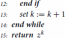
Figure 1. Performance profiles for Experiment 1. From top left to bottom right: number of total iterations, execution time, upper-level objective value, and percentage of full LM steps.

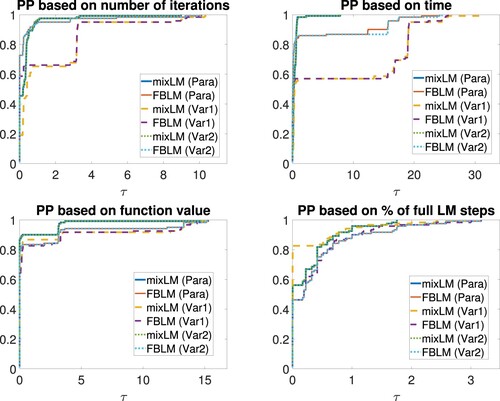
Table 1. Averaged performance indices for Experiment 1.

	mixLM	FBLM	mixLM	FBLM	mixLM	FBLM
	Para	Para	Var1	Var1	Var2	Var2
Aver. # outer iter.	1476.47	1626.61	4302.02	4301.25	1476.47	1626.61
Aver. # full LM steps	4.3970	3.7273	3.9256	3.1157	4.3970	3.7273
Aver. time	0.4748	0.4839	0.9691	1.0176	0.4702	0.4840
# Term=0	13	16	52	52	13	16
# Term=1	63	56	61	49	63	56
# Term=2	45	49	8	20	45	49
# optimal solution	74	71	69	68	74	71

We immediately see that the approaches Para and Var2 perform almost equally good. These methods terminate due to a small residual or stationarity of the squared FB residual in 90% of all runs, and the actual optimal solution is found in approximately 60% of all runs with slight advantages for mixLM. Let us now report on Var1. The optimal solution is found in about 57% of all runs. However, in this setting, both algorithms much more often do not terminate due to stationarity of the squared FB residual but are aborted since the maximum number of iterations is reached – the latter happens in 43% of the runs. Often, both algorithms seem to be close (but not too close) to a stationary point of the squared FB residual in this case, but this is not detected by our termination criterion. For a better overview, Figure 2 illustrates the termination behaviour of all six methods. 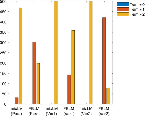Coming back to an overall comparison, mixLM in setting Para converges to the global minimizer of the problem for starting points $(x,y)$ chosen from $\left(\right\{0,\dots ,10\}\times \{0,\dots ,5\left\}\right)\cup \left(\right\{5,\dots ,10\}\times \{-2\left\}\right)\cup \left(\right\{9,10\}\times \{-3\left\}\right).$In most of the associated runs, a total number of 6 to 10 iterations is performed out of which almost all are full LM steps, i.e. we observe local fast convergence in our experiments. Related phenomena can be observed for the remaining five approaches. Particularly, despite the absence of any theoretical guarantees, local fast convergence is present in the variable settings described in Section 5.1.2. More precisely, we observed that whenever our algorithms approach the global minimizer, then this happens in a few number of full LM steps, and the convergence is, indeed, quadratic. The large average number of iterations documented in Table 1 results from the fact that whenever the algorithms do not approach the global minimizer, they tend to get stuck in stationary points of the squared residual which are approached by slow gradient steps. Typically, the algorithms are aborted in this situation since the maximum number of iterations is reached. The performance profiles in Figure 1 indicate that settings Para and Var2 are superior to Var1 when the total number of iterations and execution time are investigated. Recalling that Var1 does not stop until the maximum number of iterations is reached in comparatively many runs, its (averaged) running time is twice as large as for Para and Var2. We note that mixLM (even in setting Var1) performs more full LM steps than FBLM, see Table 1 as well. For more than 80% of all starting points, mixLM in setting Var1 carries out the highest number of full LM steps among the six methods which we are comparing here. However, there are some critical instances where, in the setting Var1, comparatively many gradient steps are done, which explains the numbers in Table 1. All this is in line with the above comments, and also extends to the computed upper-level objective value, although one has to be careful as all six methods compute the global minimizer almost equally often. However, Var1 ends up in points with comparatively high objective value in much more runs than the other two settings. Taking a look at the averaged numbers in Table 1, we observe that mixLM performs slightly quicker than FBLM for all three settings. Furthermore, mixLM finds the global minimizer more often than FBLM. The highest number of total iterations can be observed for FBLM in setting Var1.

Figure 2. Reason for termination for Experiment 1.

Experiment 2 We consider the bilevel optimization problem $\underset{x,y}{min}\frac{1}{2}\Vert y-y_{\text{o}}{\Vert }^2\text{s.t.}x\ge 0,{\mathtt{e}}^{\mathrm{\top }}\mathtt{x}\ge {\mathtt{e}}^{\mathrm{\top }}{\mathtt{b}}^{\text{dem}}\mathtt{,}\mathtt{y}\in \mathtt{S}\mathtt{\left(}\mathtt{x}\mathtt{\right)}$where $S:{\mathbb{R}}^n\rightrightarrows {\mathbb{R}}^{n\times \ell }$ is the solution mapping of the parametric transportation problem (TR$(x)$) $\begin{array}{rlrlr}\underset{y}{min}\sum _{i=1}^n\sum _{j=1}^{\ell }{c}_{\mathrm{ij}}{y}_{\mathrm{ij}}\text{s.t.}\sum _{j=1}^{\ell }{y}_{\mathrm{ij}}& \le x_i& & (i=1,\dots ,n),& \\ \sum _{i=1}^n{y}_{\mathrm{ij}}& \ge b_j^{\text{dem}}& & (j=1,\dots ,\ell ),& \\ y& \ge 0.& & & \end{array}$(TR$(x)$) Here, $\ell \in \mathbb{N}$ is a positive integer, $b^{\text{dem}}\in {\mathbb{N}}^{\ell }$ is an integer vector modelling the minimum demand of the ℓ consumers, and $c\in [0,1{]}^{n\times \ell }$ is a cost matrix. In (TR(x)), the parameter $x\in {\mathbb{R}}^n$ represents the offer provided at n warehouses which is unknown and shall be reconstructed from a given (noisy) transportation plan $y_{\text{o}}\in {\mathbb{R}}^{n\times \ell }$. For our experiments, we chose n: = 5, $\ell :=7$, and relied on the data matrices given in [64, Appendix]. As mentioned in [64], the best known solution of this bilevel optimization problem comes along with an upper-level objective value of $5.07\cdot {10}^{-4}$.

All six methods were tested based on a collection of 500 random starting points which were created in the following way. For the construction of the pair $(x,y)$, the components of x are chosen randomly from the interval $[1,10]$ while the components of y are chosen randomly from $[0,10]$, based on a uniform distribution, respectively. The associated multiplier vectors as well as ζ in setting Var2 are defined as in our first experiment. For our algorithms, we chose a maximum number of ${10}^4$ iterations, and we made use of the following values for all appearing parameters: q: = 0.9, ${\tau }_{\text{abs}}:={10}^{-4}$, ${\tau }_{\text{abs}}^{\text{stat}}:={10}^{-3}$, $\text{β}:=0.9$, $\sigma :=0.4$, ${\gamma }_1:={10}^{-4}$, ${\gamma }_2:=0.05$, and ${\rho }_1:={\rho }_2:=\rho :={10}^{-4}$. The resulting performance profiles and averaged performance indices are documented in Figure 3 and Table 2.

Figure 3. Performance profiles for Experiment 2. From top left to bottom right: number of total iterations, execution time, upper-level objective value, and percentage of full LM steps.

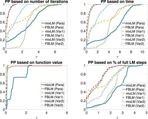
Table 2. Averaged performance indices for Experiment 2.

	mixLM	FBLM	mixLM	FBLM	mixLM	FBLM
	Para	Para	Var1	Var1	Var2	Var2
Aver. # outer iter.	97.754	10.256	54.508	10.156	67.75	20.17
Aver. # full LM steps	5.902	7.79	8.684	7.782	21.064	8.832
Aver. time	2.5777	0.0391	1.0971	0.0371	0.9610	0.1198
# Term=0	1	0	0	0	0	0
# Term=1	32	301	0	142	0	421
# Term=2	467	199	500	358	500	79
# approx. optimal	111	397	0	162	411	378

From Figure 3, it is easy to see that FBLM performs better than mixLM considering the total number of iterations, execution time, and the percentage of full LM steps although FBLM in setting Var2 cannot challenge the same algorithm in settings Para and Var1 for these three criteria, see Table 2 as well. Our choice of ${\tau }_{\text{abs}}$ and ${\tau }_{\text{abs}}^{\text{stat}}$ caused that all six methods terminated either due to a small residual or stationarity of the squared FB residual in most of the runs. Let us point out that mixLM terminated due to stationarity of the squared FB residual in most of the runs, and the same holds true for FBLM in setting Var1, see Figure 4 as well.

Figure 4. Reason for termination for Experiment 2.

This, however, does not tell the full story. In the last row of Table 2, we document the number of runs where the final iterate produces an upper level objective value between $5.06\cdot {10}^{-4}$ and $5.08\cdot {10}^{-4}$, i.e. we count the number of runs where a point is produced whose associated upper-level function value is close to the best known one (below, we will refer to such points as reasonable). As it turns out, mixLM in setting Var1 is not competitive at all in this regard. Indeed, this method most often terminates in points possessing upper-level objective value around $4.07\cdot {10}^{-4}$ and norm of the FB residual around ${10}^{-5}$. We suspect that this method tends to get stuck in stationary points of the squared FB residual which are not feasible for the inverse transportation problem. Hence, the performance profile which monitors the upper-level objective value in Figure 3 is of limited meaningfulness. The situation is far better for FBLM where reasonable points are computed much more frequently, although it has to be mentioned that the settings Para (79% reasonable) and Var2 (76% reasonable) again outrun Var1 (32% reasonable) in this regard. Interestingly, mixLM in setting Var2 always terminated due to a small value of the squared FB residual, but produced reasonable points in more than 82% of all runs. An individual fine tuning of the parameters for the settings Para, Var1, and Var2 may lead to more convincing termination reasons, but we abstained from it for a better comparison of all methods under consideration. The performance profiles in Figure 3 show that FBLM in the settings Para and Var1 are superior to Var2, and when only computed function values are taken into account, then, for the price of higher computation time, mixLM in setting Var2 is acceptable as well.

Let us note that (22(22a) $\begin{array}{rl}\mathrm{\nabla F}(\overline{x},\overline{y})+G^{\prime }(\overline{x},\overline{y}{)}^{\mathrm{\top }}\mu +g^{\prime }(\overline{x},\overline{y}{)}^{\mathrm{\top }}(\nu -\lambda \hat{\nu })& =0,\end{array}$(22a) ) turns out to be an over-determined mixed linear complementarity system in the particular setting considered here and, thus, a certain error bound condition is present. In the light of available literature on smooth LM methods, see e.g. [66], this could be a reason for the observed local fast convergence for a large number of starting points, although we did not prove such a result in this paper. Furthermore, it has to be observed that a reformulation via Var2 abrogates linearity of the system, but we obtained the best results in this setting when convergence to reasonable points is the underlying criterion.

Summary Let us briefly summarize that our experiments visualized competitiveness of the settings Para and Var2, while setting Var1 has turned out to come along with numerical disadvantages in both experiments. While, in our first experiment, there was no significant difference between Para and Var2, our second (and, by far, more challenging) experiment revealed that Var2 also could have some benefits over Para. Our experiments do not indicate whether it is generally better to apply mixLM or FBLM, but at least we can suggest that whenever the parameter λ is unknown, then it might be reasonable to apply mixLM in setting Var2 to obtain good solutions.

6. Concluding remarks

In this paper, we exploited the concept of Newton-differentiability in order to design a nonsmooth Levenberg–Marquardt method for the numerical solution of over-determined nonsmooth equations. Our method possesses desirable local convergence properties under reasonable assumptions and may be applied in situations where the underlying nonsmooth mapping is even discontinuous. We applied this idea to over-determined mixed nonlinear complementarity systems where a suitable globalization is possible via gradient steps with respect to the squared norm of the residual induced by the Fischer–Burmeister function. However, we investigated the method in two different flavors regarding the computation of the Levenberg–Marquardt direction namely via a residual given in terms of the maximum function on the one hand and in terms of the Fischer–Burmeister function on the other hand. For both methods, global convergence results have been derived, and assumptions for local fast convergence have been specified. Our analysis recovers the impressions from [9], obtained in a slightly different framework, that the approach via the maximum residual works under less restrictive assumptions. Finally, we applied these globalized nonsmooth Levenberg–Marquardt methods in order to solve bilevel optimization problems numerically. Theoretically, we were in position to verify local fast convergence of both algorithms under less restrictive assumptions than those ones stated in the literature which among others assume strict complementarity, see [41, Section 3]. Some numerical experiments were discussed in order to visualize interesting computational features of this approach.

Our theoretical and numerical investigation of bilevel optimization problems solely focused on the optimistic approach, but it might be also possible to address (similarly over-determined) stationarity systems related to pessimistic bilevel optimization via a similar approach. Next, we would like to point the reader's attention to the fact that the (inherent) inner semicontinuity assumption on the solution mapping in Lemma 5.1, see Remark 5.2 as well, is comparatively strong and may fail in many practically relevant scenarios. However, it is well known from the literature that in the presence of so-called inner semicompactness, which is inherent whenever the solution mapping is locally bounded, slightly more general necessary optimality conditions can be derived which comprise additional geometric constraints of polyhedral type addressing the multipliers, see e.g. [49, Theorem 4.9]. For the numerical solution of this stationarity system, a numerical method would be necessary which is capable of solving an over-determined system of equations subject to polyhedral constraints where either the polyhedral constraint set is not convex or the equations are non-smooth. Exemplary, we refer the interested reader to [67–69] for examples of such methods. In the future, it needs to be checked how these methods apply to the described setting of bilevel optimization, and how the assumptions for local fast convergence can be verified in this situation. Yet another way to extend our approach to more general bilevel optimization problems could be to consider the combined reformulation of bilevel optimization problems which merges the value function and Karush–Kuhn–Tucker reformulation, see [43]. A potential associated stationarity system can be reformulated as an overdetermined system of discontinuous nonsmooth equations which, similar as in [37], still can be solved with the aid of the nonsmooth Levenberg–Marquardt method developed in Section 3 as the latter one is reasonable for functions which are merely calm at their roots, and this property is likely to hold, see [37, Lemma 3.3(d)]. Let us also mention that it would be interesting to study whether an error bound condition is enough to yield local fast convergence of Algorithms 4.5 and 4.11 even in the nonsmooth setting, see [66] for the analysis in the smooth case. Furthermore, it remains to be seen whether some reasonable conditions can be found which guarantee local fast convergence of our algorithms when applied to stationarity systems of bilevel optimization problems where the multiplier associated with the value function constraint is treated as a variable, see Section 5.1.2.

Disclosure statement

No potential conflict of interest was reported by the author(s).

References

- Qi L. Convergence analysis of some algorithms for solving nonsmooth equations. Math Oper Res. 1993;18(1):227–244. https://doi.org/10.1287/moor.18.1.227
- Qi L, Sun J. A nonsmooth version of Newton's method. Math Program. 1993;58:353–367. https://doi.org/10.1007/BF01581275
- Mifflin R. Semismooth and semiconvex functions in constrained optimization. SIAM J Control Optim. 1977;15(6):959–972. https://doi.org/10.1137/0315061
- Galántai A. Properties and construction of NCP functions. Comput Optim Appl. 2012;52(3):805–824. https://doi.org/10.1007/s10589-011-9428-9
- Kanzow C, Yamashita N, Fukushima M. New NCP-functions and their properties. J Optim Theory Appl. 1997;94(1):115–135. https://doi.org/10.1023/A:1022659603268
- Sun D, Qi L. On NCP-functions. Comput Optim Appl. 1999;13(1):201–220. https://doi.org/10.1023/A:1008669226453
- Fischer A. A special Newton-type optimization method. Optimization. 1992;24(3-4):269–284. https://doi.org/10.1080/02331939208843795
- De Luca T, Facchinei F, Kanzow C. A semismooth equation approach to the solution of nonlinear complementarity systems. Math Program. 1996;75:407–439. https://doi.org/10.1007/BF02592192
- De Luca T, Facchinei F, Kanzow C. A theoretical and numerical comparison of some semismooth algorithms for complementarity problems. Comput Optim Appl. 2000;16:173–205. https://doi.org/10.1023/A:1008705425484
- Facchinei F, Kanzow C. A nonsmooth inexact Newton method for the solution of large-scale nonlinear complementarity problems. Math Program. 1997;76:493–512. https://doi.org/10.1007/BF02614395
- Kojima M, Shindo S. Extensions of Newton and Quasi-Newton methods to systems of PC1 equations. J Oper Res Soc Japan. 1986;29(4):352–374. https://doi.org/10.15807/JORSJ.29.352
- Kummer B. Newton's method for non-differentiable functions. In: Guddat J, Bank B, Hollatz H, Kall P, Klatte D, Kummer B, Lommatzsch K, Tammer K, Vlach M, Zimmermann K, editors. Advances in mathematical optimization. Berlin: Akademie-Verlag; 1988. p. 114–125. https://doi.org/10.1515/9783112479926-011
- Kummer B. Newton's method based on generalized derivatives for nonsmooth functions: convergence analysis. In: Oettli W, Pallaschke D, editors. Advances in optimization. Springer: Berlin; 1992. p. 171–194. https://doi.org/10.1007/978-3-642-51682-5_12
- Pang J-S. Newton's method for B-differentiable equations. Math Oper Res. 1990;15(2):311–341. https://doi.org/10.1287/moor.15.2.311
- Robinson SM. Newton's method for a class of nonsmooth functions. Set-Valued Anal. 1994;2:291–305. https://doi.org/10.1007/BF01027107
- Facchinei F, Pang J-S. Finite-dimensional variational inequalities and complementarity problems. New York: Springer; 2003. https://doi.org/10.1007/b97543
- Izmailov AF, Solodov MV. Newton-type methods for optimization and variational problems. New York: Springer; 2014. https://doi.org/10.1007/978-3-319-04247-3
- Klatte D, Kummer B. Nonsmooth equations in optimization. regularity, calculus, methods and applications. Boston: Kluwer Academic; 2002. https://doi.org/10.1007/b130810
- Jiang H. Global convergence analysis of the generalized Newton and Gauss–Newton methods of the Fischer–Burmeister equation for the complementarity problem. Math Oper Res. 1999;24(3):529–543. https://doi.org/10.1287/moor.24.3.529
- Kanzow C, Petra S. On a semismooth least squares formulation of complementarity problems with gap reduction. Optim Methods Softw. 2004;19(5):507–525. https://doi.org/10.1080/10556780410001683096
- Ma C, Wang C. A nonsmooth Levenberg–Marquardt method for solving semi-infinite programming problems. J Comput Appl Math. 2009;230(2):633–642. https://doi.org/10.1016/j.cam.2009.01.004
- Qi L, Wu S-Y, Zhou G. Semismooth Newton methods for solving semi-infinite programming problems. J Glob Optim. 2003;27:215–232. https://doi.org/10.1023/A:1024814401713
- Chen C, Mangasarian OL. A class of smoothing functions for nonlinear and mixed complementarity problems. Comput Optim Appl. 1996;5:97–138. https://doi.org/10.1007/BF00249052
- Daryina AN, Izmailov AF, Solodov MV. A class of active-set Newton methods for mixed complementarity problems. SIAM J Optim. 2005;15(2):409–429. https://doi.org/10.1137/S105262340343590X
- Huang C, Wang S. A penalty method for a mixed nonlinear complementarity problem. Nonlinear Anal Theory Methods Appl. 2012;75(2):588–597. https://doi.org/10.1016/j.na.2011.08.061
- Kanzow C. Global optimization techniques for mixed complementarity problems. J Glob Optim. 2000;16:1–21. https://doi.org/10.1023/A:1008331803982
- Li D, Fukushima M. Smoothing Newton and quasi-Newton methods for mixed complementarity problems. Comput Optim Appl. 2000;17:203–230. https://doi.org/10.1023/A:1026502415830
- Monteiro RDC, Pang J-S. Properties of an interior-point mapping for mixed complementarity problems. Math Oper Res. 1996;21(3):629–654. https://doi.org/10.1287/moor.21.3.629
- Gfrerer H, Outrata JV. On a semismooth* Newton method for solving generalized equations. SIAM J Optim. 2021;31(1):489–517. https://doi.org/10.1137/19M1257408
- Brokate M, Ulbrich M. Newton differentiability of convex functions in normed spaces and of a class of operators. SIAM J Optim. 2022;32(2):1265–1287. https://doi.org/10.1137/21M1449531
- Chen X, Nashed Z, Qi L. Smoothing methods and semismooth methods for nondifferentiable operator equations. SIAM J Numer Anal. 2000;38(4):1200–1216. https://doi.org/10.1137/S0036142999356719
- Hintermüller M, Ito K, Kunisch K. The primal-dual active set strategy as a semismooth Newton method. SIAM J Optim. 2002;13(3):865–888. https://doi.org/10.1137/s1052623401383558
- Ito K, Kunisch K. Lagrange multiplier approach to variational problems and applications. Philadelphia: SIAM; 2008. https://doi.org/10.1137/1.9780898718614
- Schiela A. A simplified approach to semismooth Newton methods in function space. SIAM J Optim. 2008;19(3):1417–1432. https://doi.org/10.1137/060674375
- Ulbrich M. Semismooth Newton methods for operator equations in function spaces. SIAM J Optim. 2002;13(3):805–841. https://doi.org/10.1137/s1052623400371569
- Ulbrich M. Semismooth newton methods for variational inequalities and constrained optimization problems in function spaces. Philadelphia: SIAM; 2011. https://doi.org/10.1137/1.9781611970692
- Harder F, Mehlitz P, Wachsmuth G. Reformulation of the M-stationarity conditions as a system of discontinuous equations and its solution by a semismooth Newton method. SIAM J Optim. 2021;31(2):1459–1488. https://doi.org/10.1137/20M1321413
- Dempe S. Foundations of bilevel programming. Dordrecht: Kluwer; 2002. https://doi.org/10.1007/b101970
- Dempe S, Kalashnikov V, Pérez-Valdéz G, et al. Bilevel programming problems – theory, algorithms and applications to energy networks. Berlin: Springer; 2015. https://doi.org/10.1007/978-3-662-45827-3
- Fischer A, Zemkoho AB, Zhou S. Semismooth Newton-type method for bilevel optimization: global convergence and extensive numerical experiments. Optim Methods Softw. 2022;37(5):1770–1804. https://doi.org/10.1080/10556788.2021.1977810
- Fliege J, Tin A, Zemkoho AB. Gauss–Newton-type methods for bilevel optimization. Comput Optim Appl. 2021;78:793–824. https://doi.org/10.1007/s10589-020-00254-3
- Tin A, Zemkoho AB. Levenberg–Marquardt method and partial exact penalty parameter selection in bilevel optimization. Optim Eng. 2023;24:1343–1385. https://doi.org/10.1007/s11081-022-09736-1
- Ye JJ, Zhu DL. New necessary optimality conditions for bilevel programs by combining the MPEC and value function approaches. SIAM J Optim. 2010;20(4):1885–1905. https://doi.org/10.1137/080725088
- Tseng P. Growth behavior of a class of merit functions for the nonlinear complementarity problem. J Optim Theory Appl. 1996;89(1):17–37. https://doi.org/10.1007/bf02192639
- Facchinei F, Soares J. A new merit function for nonlinear complementarity problems and a related algorithm. SIAM J Optim. 1997;7(1):225–247. https://doi.org/10.1137/S1052623494279110
- Zemkoho AB. Solving ill-posed bilevel programs. Set-Valued Var Anal. 2016;24:423–448. https://doi.org/10.1007/s11228-016-0371-x
- Clarke FH. Optimization and nonsmooth analysis. Philadelphia: SIAM; 1990. https://doi.org/10.1137/1.9781611971309
- Dempe S, Dutta J, Mordukhovich BS. New necessary optimality conditions in optimistic bilevel programming. Optimization. 2007;56(5-6):577–604. https://doi.org/10.1080/02331930701617551
- Dempe S, Zemkoho AB. The generalized Mangasarian–Fromovitz constraint qualification and optimality conditions for bilevel programs. J Optim Theory Appl. 2011;148(1):46–68. https://doi.org/10.1007/s10957-010-9744-8
- Mordukhovich BS, Nam NM, Phan HM. Variational analysis of marginal functions with applications to bilevel programming. J Optim Theory Appl. 2012;152(3):557–586. https://doi.org/10.1007/s10957-011-9940-1
- Tanino T, Ogawa T. An algorithm for solving two-level convex optimization problems. Int J Syst Sci. 1984;15(2):163–174. https://doi.org/10.1080/00207728408926552
- Henrion R, Jourani A, Outrata J. On the calmness of a class of multifunctions. SIAM J Optim. 2002;13(2):603–618. https://doi.org/10.1137/S1052623401395553
- Rockafellar RT, Wets RJ-B. Variational analysis. Berlin: Springer; 1998. https://doi.org/10.1007/978-3-642-02431-3
- Ye JJ, Wu S-Y. First order optimality conditions for generalized semi-infinite programming problems. J Optim Theory Appl. 2008;137(2):419–434. https://doi.org/10.1007/s10957-008-9352-z
- Ye JJ, Zhu DL. Optimality conditions for bilevel programming problems. Optimization. 1995;33(1):9–27. https://doi.org/10.1080/02331939508844060
- Henrion R, Surowiec TM. On calmness conditions in convex bilevel programming. Appl Anal. 2011;90(6):951–970. https://doi.org/10.1080/00036811.2010.495339
- Ke R, Yao W, Ye JJ, et al. Generic property of the partial calmness condition for bilevel programming problems. SIAM J Optim. 2022;32(2):604–634. https://doi.org/10.1137/20M1371403
- Mehlitz P, Minchenko LI, Zemkoho AB. A note on partial calmness for bilevel optimization problems with linearly structured lower level. Optim Lett. 2021;15:1277–1291. https://doi.org/10.1007/s11590-020-01636-6
- Zemkoho AB, Zhou S. Theoretical and numerical comparison of the Karush–Kuhn–Tucker and value function reformulation in bilevel optimization. Comput Optim Appl. 2021;78:625–674. https://doi.org/10.1007/s10589-020-00250-7
- Robinson SM. Some continuity properties of polyhedral multifunctions. In: König H, Korte B, Ritter K, editors. Mathematical programming at oberwolfach. Berlin: Springer; 1981. p. 206–214. https://doi.org/10.1007/BFb0120929
- Dempe S, Mordukhovich BS, Zemkoho AB. Necessary optimality conditions in pessimistic bilevel programming. Optimization. 2014;63(4):505–533. https://doi.org/10.1080/02331934.2012.696641
- Mehlitz P, Zemkoho AB. Sufficient optimality conditions in bilevel programming. Math Oper Res. 2021;46(4):1573–1598. https://doi.org/10.1287/moor.2021.1122
- Zhou S, Zemkoho AB, Tin A. BOLIB: bilevel optimization LIBrary of test problems. In: Dempe S, Zemkoho AB, editors. Bilevel optimization: advances and next challenges. Cham: Springer International; 2020. p. 563–580. https://doi.org/10.1007/978-3-030-52119-6_19
- Mehlitz P. Asymptotic regularity for Lipschitzian nonlinear optimization problems with applications to complementarity constrained and bilevel programming. Optimization. 2023;72(1):277–320. https://doi.org/10.1080/02331934.2022.2031190
- Dolan ED, Moré JJ. Benchmarking optimization software with performance profiles. Math Program. 2002;91(2):201–213. https://doi.org/10.1007/s101070100263
- Yamashita N, Fukushima M. On the rate of convergence of the Levenberg–Marquardt method. In: Alefeld G, Chen X, editors. Topics in numerical analysis. Vienna: Springer; 2001. p. 239–249. https://doi.org/10.1007/978-3-7091-6217-0_18
- Behling R, Fischer A, Haeser G, et al. On the constrained error bound condition and the projected Levenberg–Marquardt method. Optimization. 2017;66(8):1397–1411. https://doi.org/10.1080/02331934.2016.1200578
- Facchinei F, Fischer A, Herrich M. A family of Newton methods for nonsmooth constrained systems with nonisolated solutions. Math Oper Res. 2013;77:433–443. https://doi.org/10.1007/s00186-012-0419-0
- Facchinei F, Fischer A, Herrich M. An LP-Newton method: nonsmooth equations, KKT systems, and nonisolated solutions. Math Program. 2014;146:1–36. https://doi.org/10.1007/s10107-013-0676-6