Scalable Water Balances from Earth Observations (SWEO): results from 50 years of remote sensing in hydrology

ABSTRACT

Strategic planning of water management at the river-basin scale requires (1) measurement and accounting of individual hydrological processes, (2) quantification of water resources, and (3) their optimal allocation. Scalable Water Balances from Earth Observations (SWEO) is an open-access parameterization enabling automated reporting of water footprints and Sustainable Development Goal (SDG) indicators. We present its systematic arrangement and input datasets, and demonstrate its accuracy by independent riverflow measurements. We also review some achievements in remote sensing for hydrology during the last 50 years in quantifying hydrological and water management processes, flows, fluxes and changes in storage from various independent sources; and append mathematical formulations.

KEYWORDS:

• 50 years of remote sensing hydrology
• rapid water accounting
• scalable water balance
• open-access Earth observation databases
• internal calibration

Introduction

Tony Allan observed, ‘the way that we consume water is detached’ (Allan, 1997). He pointed out that the greater part of our water resources is consumed by the food supply chain. The World Economic Forum (2014) listed water scarcity as a global risk affecting business, society and the environment; Mekonnen and Hoekstra (2016) estimated that two-thirds of the global population (4.0 billion people) live under conditions of severe water scarcity at least one month of the year. The amount of water used to produce the goods, commodities and services that we rely on has been formally captured by the water footprint concept, and teams led by Allan and Hoekstra have used this concept to quantify water systems and water use at the product, field and river-basin scales (Hoekstra, 2013). Here, we focus on the water footprint per river basin.

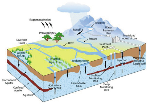
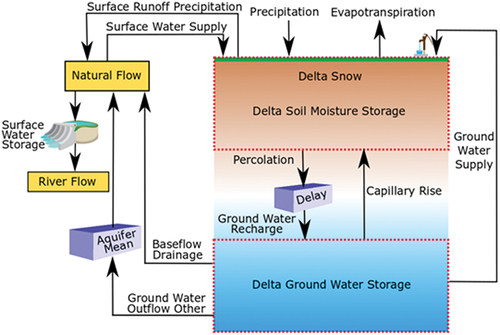
Scarcity prompts users to develop accounting systems for water resources (e.g., Bastiaanssen, 2009; Karimi et al., 2013; Molden, 1997). Financial accounts present an overview of inputs, outputs and resulting balances that provide strategic insights: the same applies to water accounting (Figure 1). However, even more so than financial accounting, accurately measuring inflows, outflows and changes in storage in water systems is fraught with difficulty (Davids et al., 2019a). For instance, it is essential to know the difference between gross and net water withdrawals, but, in many cases, it is not directly measurable – even blue water in streams, lakes and reservoirs is hard to quantify (Davids et al., 2019b). Weekly or monthly water resources budgets would be helpful in support of fundamental decisions about water allocation, but the determination of all in- and outflows is hard to do and, therefore, not often done. So, it is the exception and not the rule to have reasonably complete water balances available for decision-makers. New tools and streamlined processes for water accounting are sorely needed.

Figure 1. Physical processes in a river basin that need to be quantitatively described by water authorities for dealing with water scarcity and communications with society.

Source: https://www.alevelgeography.com/drainage-basin-hydrological-system/.

Followers of water footprints use CropWat and AquaCrop models (Steduto et al., 2009) to relate water use to food production (e.g., Chukalla et al., 2015). While these models are robust, they are typically applied at the field scale; for the water footprint of river basins, more comprehensive methods are needed. Feng et al. (2021) have reviewed the analytical tools used for water footprint analysis, including some remote sensing methods that have emerged in recent years (e.g., Madugundu et al., 2018). Shilpakar et al. (2011) estimated monthly river flow in the East Rapti basin, Nepal, from remotely sensed monthly precipitation minus evapotranspiration (P-ET) data; Bastiaanssen et al. (2014) applied P-ET pixel information to determine river flow and water withdrawals in the Nile basin; and, similarly, Poortinga et al. (2017) estimated flow in the Red River, Vietnam. Moreira et al. (2019) went a step further by merging P, ET and storage changes (ΔS) from the independent GRACE gravity mission to estimate terrestrial water balances in South America. Here, we report progress in preparing spatially distributed water balances using open-access Earth observations of P, ET and ΔS – in particular, the methods used in Scalable Water Balances from Earth Observations (SWEO) which enable the computation of consistent water balances at the river-basin scale.

50 years of remote sensing of hydrological processes (1970–2020)

Adequate water accounting systems require big datasets that are not easily available. SWEO uses globally standardized, open-access datasets: (1) to avoid dependence on unpredictable data-sharing attitudes from third parties; and (2) to alleviate any appearance of bias and potential data-sharing limitations associated with data ownership. Therefore, the results and achievements from water accounting can be shared with all relevant stakeholders. SWEO integrates Earth-observation data from the following individual hydrological processes into a vertical soil water balance for each pixel (currently either 250 or 1000 m): rainfall, snowmelt, evapotranspiration, soil moisture, water levels, surface-water change and groundwater-storage change. These data are currently available from various Earth-observation data archives (Table 1). These databases are based on recurrent satellite measurements, with time steps varying from daily to monthly. In addition, there are several data layers that, by nature, are relatively stable but essential for determining physical process, such as soil hydraulic conductivity that controls, for example, the partitioning of rainfall into surface runoff and infiltration.

Table 1. Open-access databases leveraged by Scalable Water Balances from Earth Observations.

	Spatially variable–temporally variable			Spatial variable–temporally constant
Variable	Source	Spatial (m)	Temporal (days)	Variable	Source	Spatial (m)
Precipitation	CHIRPS	5000	1	Terrain height, accumulated pixels, drainage direction	SRTM or HydroShed	90, 250 or 1000
Rainfall days	CHIRPS	1000	1	Land cover	GlobCover and MCD12Q1	300 or 500
ET0 reference	FEWS	10,000	1	Population density	GPW V4	1000
ET actual	WaPOR, SSEBop	30, 250, 1000	1	Livestock density	FAO GWL 2005	5000
Air temperature	GLDAS, MERRA or GEOS	25,000 or 50,000	0.125 or 0.25	Sand content	SoilGrids	250
LAI (MOD15A2)	MODIS	500	8	Clay content	SoilGrids	250
fPAR (MOD15A2)	MODIS	500	8	Soil organic carbon content	SoilGrids	250
Snow cover (MOD10A2)	MODIS	500	8	Bulk density	SoilGrids	250
∆S Ground Water Storage	GRACE	300,000 −400,000	30	Saturated hydraulic conductivity (Ksat)	SoilGrids	250
Water body area	JRC	30	–	Specific yield (μ)	SoilGrids	250
				Piezometric heads at start	PCR-GLOBWB	9000
				Reservoirs and dams (optional)	GRAND	Points

Precipitation (P) and snow cover

There are several rainfall products based on radar satellites, notably Tropical Rainfall Measurement Mission (TRMM) and Global Precipitation Mission (GPM). Radar emits a burst of energy that is scattered if the energy strikes an object (raindrop, snowflake, hailstone); the density of rainfall droplets and the size of these droplets affects the scattering. In combination with radar measurements, thermal radiometers onboard geostationary satellites and radar satellites measure cloud temperatures that reflect water and ice concentrations. Remotely sensed precipitation products represent larger areas than a gauge on the ground, which has advantages and disadvantages. A larger representative area is great for determining catchment and river-basin rainfall volumes, but it is hard to validate because, by definition, there is a spatial-scale mismatch with in situ measurements. Satellite remote sensing products achieve global coverage but may suffer from random errors and bias (Koutsouris et al., 2016) arising from the indirect linkage between the observed parameters and precipitation and, also, imperfect algorithms.

SWEO uses the calibrated Climate Hazard Group InfraRed Precipitation Stations (CHIRPS) database for monthly rainfall and number of rainy days, making use of radar and geostationary satellites, ground stations and terrain information (Funk et al., 2015). The grid size is 5 km and data are available continuously since 1981, which is attractive for generating time series (e.g., Paca et al., 2020). CHIRPS has been widely tested and is well accepted (Dinku et al., 2018; Hessels, 2015; Hsu et al., 2021; Nawaz et al., 2021).

Precipitation includes rainfall and snowfall. Snowfall extends the time lag between precipitation and runoff and infiltration, so needs to be quantified as a separate process. MODIS images detect snow cover and its changes (https://modis.gsfc.nasa.gov/data/dataprod/mod10.php). SWEO uses eight-day snow cover maps to detect the timing of snowmelt, which is an essential input into monthly river flow determinations, especially in cold or mountainous regions where snowfall comprises much of total precipitation. The amount of snowmelt is computed from changes in snow cover and ambient air temperatures during this period (standard equations are provided in Appendix A in the supplemental data online). SWEO has delay factors built in for the location and timing of snowmelt and the arrival of meltwater in the nearest stream. In this way, snow cover information can be used to infer which parts of CHIRPS-based precipitation can be attributed to snowfall and which to rainfall. For further information on remote sensing of snow cover products, see Hall et al. (2002), Parajka and Blöschl (2006) and Rittger et al. (2013).

Evapotranspiration (ET) (actual)

ET represents consumptive use of water. It is the second largest term of the water balance, returning about two-thirds of precipitation to the atmosphere, so it is crucial for water footprint analysis but hard to measure without advanced equipment. It is commonly assumed that weather stations measure ET. Not so. Weather stations measure the state conditions of the atmosphere which can be used to assess a reference ET of grass or alfalfa. The United Nations Food and Agriculture Organization (FAO) has adopted procedures to compute reference ET (ET₀) from a strictly defined hypothetical surface (Allen et al., 1998), but these values may deviate substantially from actual ET; several ET algorithms have been developed but only a few operational spatial databases are related to actual ET fluxes. SWEO uses ET for the water balance, and ET₀ for computing the aridity index, which is used (among other processes) to develop Budyko curves for partitioning green and blue ET (Budyko, 1974; Simons et al., 2020a).

The first scientific publications using thermal infrared satellite measurements to express evaporative cooling date from the 1960s–70s (Gates, 1964; Jackson et al., 1977; Menenti, 1980; Rosema & Fiselier, 1990; Soer, 1977). Since then, many algorithms have been developed and tested against field measurements, amongst them the Surface Energy Balance Algorithm for Land – SEBAL (Bastiaanssen & Roebeling, 1993), which has been widely adopted and that led to other energy-balance models such as the Simple Surface Energy Balance Operational model (SSEBop) (Savoca et al., 2013; Senay et al., 2014), originally developed to monitor drought and crop development for Africa but now applied globally; METRIC (Allen et al., 2007); ETWatch (Wu et al., 2008); and SAFER (Teixeira et al., 2015). Another operational ET product, GlodET (www.glodet.nebraska.edu) from the Water for Food Institute, is based on the ALEXI model (Anderson et al. 2007a, 2007b).

The latest versions of SEBAL are implemented on Google Earth Engine, so they are becoming more easily available for automated implementation (Jaafar & Mourad, 2021; Laipelt et al., 2021). In principle, 30 m SEBAL outputs could be used for high-resolution applications of SWEO, but this has yet to be tested. SWEO is agnostic in terms of ET data and can use any raster-based ET dataset.

Soil water

Soil water controls various agronomic and ecological processes. Wet soils in arid climates suggest non-precipitation sources of water in the form of irrigation, floods or shallow groundwater. Determination of soil water by remote sensing usually makes use of thermal images (often in combination with vegetation cover) or microwave imagery. Passive microwave sensors measure the very weak natural emissions of the Earth surface after making corrections for vegetation (Jackson et al., 2011; Kerr et al., 2012; Mo et al., 1982; Owe & Van de Griend, 1998; Schmugge et al., 1986). At best, near-surface soil water values can be acquired for very large pixels (12.5–50 km) with sparse vegetation. The Soil Moisture and Ocean Salinity (SMOS) satellite measures radiation emitted in the microwave L-band (1.4 GHz). The Soil Moisture Active Passive (SMAP) satellite was to combine passive and active signals (Entekhabi et al., 2010), but the active radar system is not functioning; instead, radar-based soil moisture retrieval is based on Sentinel 3 data (Ojha et al., 2021). Lekshmi et al. (2014) review the retrieval of remotely sensed soil water.

Because of the poor spatial resolution of microwave techniques and their restriction to the near-surface layer, SWEO estimates soil water from thermal infrared measurements following the principles of a relative term of ET (e.g., Hain et al., 2011) or the evaporative fraction of the surface energy balance (e.g., Bastiaanssen et al., 1997; Scott et al., 2003). Canopy temperature reflects the access of vegetation to soil water in the entire root zone, thereby probing deeper into the soil than microwave technology. Earlier soil water detection work based on thermal infrared remote sensing (e.g., Carlson, 2007; Carlson et al., 1994; Gillies & Carlson, 1995) is based on the trapezoid between surface temperature and vegetation cover. Pang et al. (2020) compiled a good review of methods to assess soil water using thermal measurements.

Groundwater storage changes

Groundwater resources can be of immense value to ecosystems, and for domestic and industrial use. Recharge resulting from the infiltration of precipitation is the main source. Groundwater storage changes (ΔS_gw) are a result of differences between groundwater inflows (predominantly recharge at the river basin scale) and outflows (withdrawals, baseflow to streams, ET from groundwater-dependent ecosystems, and inter-basin groundwater flows). Due to geological variability, these underground processes are hard to quantify without calibrated local groundwater models, so GRACE satellite data are invaluable as an independent measure of changes in water storage. GRACE measures inter-satellite range changes and their derivatives between two co-planar satellites in low-altitude, polar orbits 220 km apart, achieving global coverage every 30 days; the orbits of the two independently orbiting systems are perturbed by the Earth’s gravitational field, leading to inter-satellite range variations. Each system carries a Global Positioning System (GPS) receiver of geodetic quality and high-accuracy accelerometers to enable accurate orbit determination, spatial registration of gravity data and the estimation of gravity field models. Primarily, gravity fluctuations on land reflect storage changes of water, snow and ice. The value of GRACE data has been demonstrated in many hydrological studies (e.g., Jiang et al., 2014; Long et al., 2014; Rodell & Famiglietti, 2002; Sriwongsitanon et al., 2020). SWEO uses GRACE data from the Colorado Center for Astrodynamics Research (https://ccar.colorado.edu/grace/gsfc.html) to account for changes in groundwater storage.

Surface water storage changes

Lakes and reservoirs can store runoff to meet subsequent crop water demands. Changes in surface areas of open water bodies can be detected easily and accurately from spectral water indices (e.g., normalized difference water index – NDWI) and from radar backscatter signals. Changes of water bodies have recently been summarized into water occurrence maps (https://developers.google.com/earth-engine/datasets/catalog/JRC_GSW1_3_GlobalSurfaceWater); and attempts are being made to determine the width (perhaps, in future, flow) of large rivers (Yang et al., 2019).

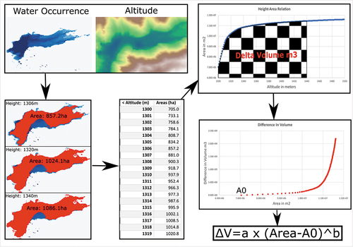
SWEO relates the relationship between open-water surface areas (A) and water elevations (L) with water volumes using information from a pre-inundation Digital Elevation Model (Figure 2). First, water occurrence data are used to identify lakes and reservoirs. Next, changes in area can be related to changes in water level (Duan & Bastiaanssen, 2013). Unique A(L) relationships for each reservoir can be mathematically integrated to arrive at volume V changes. The relationship between the volume of water storage and the surface area (i.e., V = f(A) relationship) for each lake or reservoir is determined by SWEO and used to assess monthly surface-water storage changes (ΔS_sw). As an independent validation, water-level measurements can also be taken from satellite-borne altimeter data (e.g., https://dahiti.dgfi.tum.de/en/map/). For various reasons, it is essential to make a distinction between natural water bodies that delay the natural runoff and reservoirs that provide a mechanism to store surface water for a longer period (months, years); SWEO uses the database of dams and reservoirs (GRAND) to differentiate between natural lakes and operational reservoirs (Lehner et al., 2011).

Figure 2. Remotely sensed determination of the relationship between water body surface area, water levels and water volume.

Land use

Land use influences hydrology and water management. For instance, forests intercept and consume a lot of water and can draw on shallow groundwater (McCulloch & Robinson, 1993), whereas urban areas have a completely opposite hydrological response. And hydrological processes affect land uses: for instance, cropland with sufficient but not abundant rainfall can be seasonally flooded and transformed into wetlands. SWEO uses land-use information to quantify and characterize the various services and benefits arising from consumptive use: bush and natural landscapes provide biodiversity and have reduced greenhouse gas emissions; irrigated agriculture provides jobs and food security, and also provides significant ecosystem services such as microclimate cooling, reduction of erosion and carbon capture.

SWEO uses customized land-use land cover (LULC) classes but, when dealing with global databases, it is often unavoidable to also include more generic land cover classes. At a minimum (pending the availability of more detailed LULC information), SWEO expresses water usage by means of the following classes retrieved from GlobCover (Arino et al., 2007) and MODIS (MCD12Q1): (1) bare land, (2) bushland, (3) forest, (4) pasture, (5) irrigated cereals, (6) irrigated non-cereals, (7) irrigated perennials, (8) rainfed crops, (9) other nature, (10) urban, (11) snow and ice, (12) natural water bodies, and (13) reservoirs (Table 1). When agencies have locally refined LULC information, this information can be incorporated into SWEO.

LAI and fPAR

In addition to ecosystem services, vegetation regulates the conversion of P into ET, enhances the infiltration capacity and water-holding capacity of soils, and provides food, stockfeed and fibre. SWEO uses leaf area index (LAI) information from MODIS to compute the partitioning of ET into E (evaporation) and T (transpiration). Also, interception and infiltration can be estimated from LAI and the fractional vegetation cover related to LAI. The fraction of photosynthetically active radiation (fPAR) is taken from MODIS to compute dry matter production from radiation using light-use efficiency (LUE) (Monteith, 1977).

Further reviews of the remote sensing to determine hydrological processes have been prepared by Engman and Gurney (1991), Schultz (1988), Schmugge et al. (2002), Pietroniro and Prowse (2002), Neale and Cosh (2012) and Frappart and Bourrel (2018).

SWEO parameterization

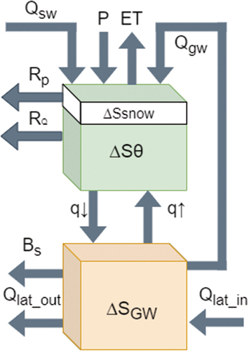
Hydrological input data are downloaded from independent satellite data archives. The risk is that each term has its own uncertainty and, by adding all terms together, an unrealistic water balance arises that is neither closed nor consistent: SWEO has a particular sequence of steps and procedures to avoid this. Each term is evaluated, bias corrected (when feasible), calibrated and tuned for conservation of mass. SWEO computes a two-layer vertical soil water balance for every pixel with a monthly time step. There is an upper soil water balance that represents the root zone with a fixed thickness of 0.5 m. Below is an unconfined shallow aquifer that represents a groundwater bucket with lateral exchanges. All flows between the two layers are assumed to be vertical. The upper soil water balance for the root zone is defined as:

$\mathrm{P}+{\mathrm{Q}}_{\mathrm{s}\mathrm{w}}+{\mathrm{Q}}_{\mathrm{g}\mathrm{w}}+{\mathrm{q}}^{\uparrow }=\mathrm{E}\mathrm{T}+{\mathrm{R}}_{\mathrm{P}}+{\mathrm{R}}_{\mathrm{Q}}+{\mathrm{q}}^{\downarrow }+\mathrm{\Delta }{\mathrm{S}}_{\theta }+\mathrm{\Delta }{\mathrm{S}}_{\mathrm{s}\mathrm{n}\mathrm{o}\mathrm{w}}$

where P is precipitation, Q_SW is the surface water supply, Q_GW is the groundwater supply, q^↑ is the capillary rise from shallow water tables, ET is the actual evapotranspiration, R_P is the surface runoff due to precipitation, R_Q is the surface runoff from water supply, q^↓ is the percolation, ∆S_θ is the change of soil moisture storage, and ∆S_snow describes the storage changes of snow. Figure 3 presents these major processes where the Δ sign reveals incremental values related to Q_sw and Q_gw. These blue arrows originate both from natural (e.g., seepage, flood) and anthropogenic (e.g., pumping) water supplies.

Figure 3. Vertical soil water balance applied to any pixel.

Due to the importance of consumptive use, actual evapotranspiration ET is considered in more detail. One breakdown is to separate ET into the physically different processes E + T + I, where E is the evaporation from soil and water surfaces, T is the evaporation through stomata and I is the evaporation from interception; another is into the source of water, namely ET from rainfall (ET_green) and non-rainfall sources (ET_blue).

Runoff from precipitation (R_p) denotes snowmelt and overland flow. There is also runoff R_Q from the water supply (Q_sw + Q_gw) that is specified a priori for different types of land use such as the leakage from a water utility or the tail water of an irrigation furrow. The groundwater bucket receives percolation water which can be considered as recharge of the shallow aquifer. The water balance of the shallow aquifer is defined as:

${\mathrm{q}}^{\downarrow }+{\mathrm{Q}}_{\mathrm{l}\mathrm{a}\mathrm{t}\mathrm{\_}\mathrm{i}\mathrm{n}}={\mathrm{Q}}_{\mathrm{g}\mathrm{w}}+{\mathrm{B}}_{\mathrm{S}}+{\mathrm{Q}}_{\mathrm{l}\mathrm{a}\mathrm{t}\mathrm{\_}\mathrm{o}\mathrm{u}\mathrm{t}}{+\mathrm{q}}^{\uparrow }+\mathrm{\Delta }{\mathrm{S}}_{\mathrm{G}\mathrm{W}}$

where q^↓ is the recharge from leaking fields, Q_lat is the lateral groundwater flow, Q_gw is the groundwater abstraction by crops and groundwater dependent ecosystems, B_S is the base flow towards the main river for provision of dry season flow, q^↑ is capillary rise, and ∆S_GW is the changes of groundwater storage. Recharge q^↓ occurs from snow-covered land being saturated with water, forests, rivers, lakes and from irrigated land. SWEO considers recharge to be a three-month moving average of percolation water leaving the root zone because it takes time before moisture touches the zone of saturation where pores and fractures of the ground are saturated. Soil water needs to be above field capacity for generating percolation, albeit drier soils can also convey water but at a lower rate. Appendix A in the supplemental data online provides the mathematical formulation of percolation and other flows and fluxes presented in Figure 3.

Two types of bias corrections are included in SWEO. First, P is compared with individual rain gauges; bias factors can be derived to explain the difference with observations, and these factors can be inserted to modify monthly CHIRPS data. Next is the verification of the total mass balance of the river basin. Without any knowledge on internal water (re-)distribution in the basin, it can be stated in general that a bulk water balance always applies:

$\mathrm{\Sigma }\mathrm{Q}=\mathrm{\Sigma }\mathrm{P}-\mathrm{\Sigma }\mathrm{E}\mathrm{T}-\mathrm{\Sigma }\mathrm{\Delta }\mathrm{S}$

where ΣQ is the net basin outflow, being the difference between transboundary inflow (i.e., aqueduct, aquifer) and outflow (i.e., sea, sink, aquifer). Because ΣP is bias corrected by gauges and ΣET is the second most important term that far exceeds ΣS in absolute numbers, SWEO introduces a bias correction for ΣET to make the balance. A prerequisite for applying this second bias correction is that ΣQ is measured. In the absence of outflow measurements, at best the longer term ΣQ term can be approximated from global hydrological models or other sources of information. The bias correction for ΣET will, for simplicity, be applied to any pixel and to any month. This is realistic as the equation for net radiation can have a systematic deviation that applies to any pixel. A constraint is built in to prevent monthly ET exceeding 250 mm/month. Hence, ΣP and ΣET at the river basin scale are always congruent with ΣS and ΣQ.

With P and ET being bias corrected for every pixel, information on P-ET can be deployed to obtain first insights into the location of net water-generating areas (P > ET) and net water-consuming areas (P < ET). Figure 4 is an example from Afghanistan showing mountains and water divides with P-ET > 500 mm/yr simultaneously with irrigated and wetland areas with P-ET ~ –1000 mm/yr. Water must move from positive to negative P-ET values, and where river topography cannot explain this, interflow and groundwater flows must take care of this lateral transport. Hence, the vertical pixel columns are hydrologically connected through streams and aquifers.

Figure 4. Annual scale values of P – ET in Afghanistan during 2015.

Note: Positive values represent net water-generating areas; and negative values are net water consumers (wetlands, irrigation systems).

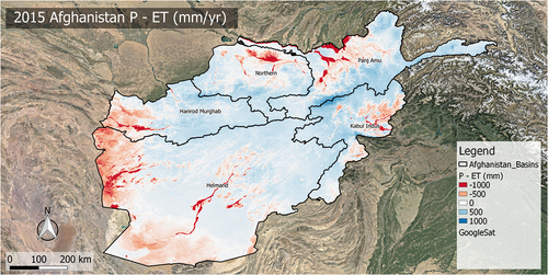
Figure 5. Schematic coupling of various components of Scalable Water Balances from Earth Observations in the regional basin context.

Surface runoff (R_P + R_Q) is routed from each pixel to the nearby stream using topographical information. The same occurs with baseflow B_S that is, by definition, an extra source of water to the river system. However, B_S cannot drain all excess groundwater to rivers because it depends on hydraulic heads and hydraulic conductivity (see Appendix A in the supplemental data online). There is a maximum capacity to B_S that cannot be exceeded.

With the vertical soil and groundwater bucket for every pixel being determined, the water resources of aggregated areas such as natural catchments, sub-basins, irrigation schemes or administrative units can be quantified. Figure 5 shows the schematic coupling of the vertical pixel based balance and the regional basin including also horizontal components. In the absence of detailed, available groundwater models, SWEO considers lateral groundwater movements Q_lat in the regional context. The Q_lat sign of a pixel can be positive or negative depending on other terms of the groundwater bucket. Because groundwater storage changes ∆S_GW are measured by large GRACE pixels and, thus defined, a lateral groundwater process is required to obtain an equilibrium between all smaller pixels, a mixed-cell approach of all pixel-based groundwater buckets is applied to check whether there is an equilibrium. If the balance is neutral, then Q_lat from SWEO is considered as an assessment of local lateral groundwater movement without any geohydrological basis. If not in balance, B_S is enhanced to a certain maximum by syphoning groundwater to streams. If still not in balance, the separation of Q_sw and Q_gw will be adjusted until Q_lat at the regional scale (aquifer level) is zero. This is another important calibration process to get realistic groundwater balances. A key assumption in this process is that recharge is reasonably good (and has been internally calibrated from green water pixels; see the next section).

SWEO computes river flow for every 250 m reach by accumulating surface runoff (R_p and R_Q) and baseflow B_S from the nearest pixels; in general, though not in drylands, river flow increases from the upstream to the downstream ends of the basin. Lakes and reservoirs create a storage-and-release system that is included in the flow accumulation: ΔS_sw are computed from the V(A) relationship that varies with each surface-water body. The complexity of this system can be defined by the user by defining the minimum size of a water body that should be considered in SWEO.

Surface water is withdrawn in transit by various agro-ecosystems. These withdrawals diminish flow and large flood plains and wetlands or irrigation systems can reduce river flow to virtually nothing. So, it is essential to have a number of checkpoints for actual flow; in case of a mismatch of river flow, corrections on the ratio of surface water (Q_sw) versus groundwater supply (Q_gw) for different land-use classes are introduced. The assessments of various sinks and sources make it feasible to reconstruct a hydrograph at any reach. In the case of natural catchments with small withdrawals and supplies, corrections on infiltration and runoff are introduced.

The calculation of q^↓, R_p, Q_sw and Q_gw for every pixel depends on P, ET and soil water θ. To simplify the process, first q^↓ and R_p are computed for pixels where water supply can be safely excluded, hence Q_sw and Q_gw are zero for this special group of pixels. This occurs when P > ET: they are also known as green water pixels. The notion of green water was introduced by Falkenmark and Rockström (2006, p. 130) to better understand agro-ecosystems that need no water supply other than ‘water from precipitation that is stored in the root zone of the soil and evaporated, transpired or incorporated by plants’. This definition is followed in SWEO. For green water pixels, q^↓ can be approximated as P-ET – R_p – ΔS. ET_green is a natural process that is hard to change (only by land-use changes). In SWEO, a first estimation of ET_green is computed from the Budyko curve that prescribes the breakdown of gross rainfall into runoff and ET_green using the aridity index. This will give a first separation between rainfed and irrigated pixels required to calculate q^↓. A more precise ET_green value can be computed from a separated soil water balance that does not have any other water source then P (Dogrul et al., 2017). Therefore, one soil water balance in SWEO is only for green water determination, and the same pixel has a second soil water balance for all inflows and outflows.

The counterpart ET_blue relates to water supply from surface water systems (streams, rivers, lakes, reservoirs, wetlands, lagoons) and groundwater systems (unsaturated zone, unconfined and confined aquifers). Floods, irrigation, seepage, interflow, capillary rise and deep-rooting plants all supply water to vegetation that evaporates into the atmosphere. The water footprint network defines blue water as ‘water that has been sourced from surface or groundwater resources and is either evaporated, incorporated into a product or taken from one body of water and returned to another, or returned at a different time’. SWEO defines ET_blue as the incremental consumptive use due to water supply from a piped utility, hydrants, irrigation canal, river inflow, flood, interflow, capillary rise, perched water table, groundwater pumping or direct withdrawal from deep rooting systems. (Note: ET_blue is computed as ET – ET_green, so any error in ET_green is translated into ET_blue.) The isolation of computing percolation q^↓ and surface runoff R_p from ET_green pixels, followed by determination of surface water Q_sw and groundwater supplies Q_gw is a practical method to solve terms of the water balance that cannot be derived from Earth observations otherwise.

SWEO case studies

Some national-scale hydrology models may serve in national water resources plans. However, hardly any river basins have their own models, and water resources planners have to rely on open-access data. Most hydrological models focus on P and river flow. They are not suitable to describing complex irrigation, wetland, bushland and forest hydrological processes, being the major users of renewable water resources. Against this background, the FAO and TUDelft have been involved in setting up SWEO studies for different basins (Table 2).

Table 2. Scalable Water Balances from Earth Observations case studies completed. In most cases the hydrological period 2003–19 was analysed.

Countries/region	River basin
Pakistan	Indus
Afghanistan	All basins
Central Asia	Syr Darya
Myanmar	Irrawaddy
Palestine–Israel	Jordan basin and mountain aquifer
Chile	Seven selected basins

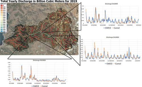
The success of merging different hydrology terms into a consistent, calibrated water balance can be checked with independent field measurements; river discharge at key locations is suitable information for such validation. Note that river flow is not a standard SWEO input parameter but infiltration, baseflow, groundwater withdrawals and surface water withdrawals are tuned to match the longer term flow at strategic locations. Figures 6 and 7 demonstrate the accuracy attainable following the standard SWEO internal calibrations.

Figure 6. Estimated monthly inflow into the Shardara reservoir based on Scalable Water Balances from Earth Observations water accounting and discharge measurements by KhazHydroMet (Kazakhstan).

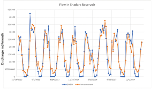
Figure 7. Estimated and measured river flow at three key discharge stations with longer term records from the Aconcagua River.

Figure 6 shows the predicted inflow into Shardara reservoir, a key reservoir in the transboundary Syr Darya River system. Inflow at this point is of paramount importance for Kazakhstan, and depends on excess water from Kyrgyzstan and other countries. The graphs show good agreement of monthly flows; the only difference is a systematically higher inflow measured during the low-flow season, which suggests that baseflow B_S should be increased or groundwater abstractions decreased to obtain a more exact match.

The second case covers three strategic discharge stations on the Aconcagua River (Chile). In this case, low flow is predicted satisfactorily, so baseflow was apparently good. Months with peak flow are determined well, and this confirms that spatio-temporal P-ET data and surface runoff R_p are accurate. Also, the partitioning into surface runoff and the withdrawals for irrigation and other water use sectors must be rather accurate, otherwise the flow at particular points would not match.

These two examples demonstrate that river flow can be rather well reproduced indirectly from satellite measurements, and that SWEO can be used for various allocation analyses including withdrawals, supplies, consumptive use, non-consumptive use and recycling. This is the basis for using the information for evaluating good water management practices.

SWEO implementation in water footprint analysis of river basins

Society’s water footprint must be reduced (Allan, 2003; Chapagain et al., 2006). This will require courageous – that is, unpopular – interventions that will have to be supported by reliable water accounts: How much water do we really have available? Who is currently getting the water? Is the water used efficiently? Is it over-exploited? Can we import food grown elsewhere? Perry’s (2013) ABCDE(F) framework on water resources management is germane: the first step is the determination of the water accounts (being the capital A) that are necessary for defining longer term policies, rules, operations and laws. Withdrawals should be analytically related to caps on consumptive use, with an explicit recognition of consumptive use by ET_green and ET_blue (Yan et al., 2020).

Decisions require information on the longer term storage changes of lakes, reservoirs and aquifers, the volume of renewable water resources, natural and anthropogenic water supplies, return flows, recycling, reuse, and virtual water trade. Water-use efficiency, water productivity, water footprint, irrigation efficiency and beneficial fraction all help to evaluate whether water is used efficiently, and standard indicators are suggested by AquaStat and the Sustainable Development Goals (SDGs), both promoted by the United Nations. SWEO computes these performance indicators from water balances, vegetation photosynthesis and land use (Table 3).

Table 3. Information produced by Scalable Water Balances from Earth Observations for monthly water analysis.

Hydrology	Water management	Water resources indicators	Efficiency
P	External renewable water	Water utilization: withdrawal/available water	Water productivity
ET	Internal renewable water	Water scarcity: supply – demand	Water footprint
q^↓	Water demand	Water stress: ETpot – ETact	Irrigation efficiency
q^↑	Non-utilized outflow	Recycling factor: Σwithdrawal/Σsupply	Beneficial fraction
RP	Qsw per land use	Changes SW storage	Consumed fraction
RQ	Qgw per land use	Changes GW storage
BS	E per land use	Changes irrigated area
Qsw	T per land use	Changes wetland area
Qgw	ETgreen per land use	Groundwater dependency
Qlat	ETblue per land use
River flow	Consumptive use, domestic
Groundwater flow	Consumptive use, industry
	Consumptive use, livestock
	Consumptive use, hydropower

Conclusions

Changing precipitation patterns and increasing demands for water have created countless situations where most, if not all, available water resources are utilized and demands can no longer be met. Such water-scarce situations demand a rapid water-accounting system that quantifies hydrological and water management processes and presents them in a clear, consistent way. The accounts must include withdrawals, supplies, consumptive use and non-consumptive use whereby flows are returned into the river systems. Simultaneously, benefits such as dry matter production and the efficient use of scarce water resources should be described, including water footprints, water productivity, and efficiency and recycling coefficients. However, no standard model can produce all this information in an automated, standardized, rapid and affordable manner.

This paper discusses a breakthrough in water accounting – SWEO – that leverages spatially and temporally explicit information from open-access Earth observation databases and integrates these independent estimates of flows, fluxes and storage changes into a consistent water balance. This parameterization includes bias factors and internal calibration coefficients to ensure closure of the water budget; in situ measurements of precipitation and streamflow at one or more locations, especially the river basin outflow (in the case of streamflow), are necessary. However, this is a much-reduced data demand compared with classical methods for preparing monthly water balances and river basin profiles, and vital for water accounting in data-scarce regions such as Afghanistan or Myanmar. SWEO’s philosophy is to exploit recurrent Earth observation data to the greatest extent possible to provide accurate, timely, spatially discrete information in an automated manner using a standardized open-source model developed in Python. Over the last five years, six pilot studies with SWEO have been completed in collaboration with enthusiastic end-users. In order to broaden SWEO’s accessibility and usefulness, and to limit data bandwidth and computing requirements, the idea of implementing SWEO on Google Earth Engine has been suggested and is currently under consideration.

This paper summarizes: (1) SWEO’s essential open-access Earth observation data; (2) the primary mathematical framework; (3) related computational steps to achieve consistency through bias-corrections and calibration of typical breakdown; and (4) the partitioning of parameters (e.g., ET into E and T). Further, we validated SWEO with 17 years of river flow data in the Syr Darya and Aconcagua rivers. SWEO’s formalized data sources and workflow and its flexibility that enables customized tuning for particular conditions makes this new model applicable to a range of environmental, physiographical and anthropological conditions. Its outputs are standardized and include several SDG and AquaStat indicators. Finally, critical areas of development in future versions of SWEO include: (1) recycling and reuse of non-consumptive use (Simon et al., 2020b); (2) downscaling of the groundwater storage (because GRACE satellite pixels are very large; Miro & Famiglietti, 2018; Vishwakarma et al., 2021); and (3) inclusion of locally refined land-use information to improve reporting of water-related benefits and services.

Disclosure statement

No potential conflict of interest was reported by the authors.

Supplementary material

Supplementary data for this article can be accessed at https://doi.org/10.1080/02508060.2022.2117896

References

- Allan, J. A. (1997). Middle East water: Local and global issues. SOAS Water Issues Group, University of London.
- Allan, J. A. (2003). Virtual water – The water, food, and trade nexus. Useful concept or misleading metaphor? Water International, 28(1), 106–113. https://doi.org/10.1080/02508060.2003.9724812
- Allen, R. G., Pereira, L. S., Raes, D. S., & Smith, M. (1998). Crop evapotranspiration. Guidelines for computing crop water requirements [Irrigation and Drainage Paper 56]. FAO
- Allen, R. G., Tasumi, M., Morse, A., Trezza, R., Wright, J. L., Bastiaanssen, W., Kramber, W., Lorite, I., & Robison, C. W. (2007). Satellite-based energy balance for mapping evapotranspiration with internalized calibration (Metric) – Applications. Journal of Irrigation and Drainage Engineering, 133(4), 395–406. https://doi.org/10.1061/(ASCE)0733-9437(2007)133:4(395)
- Anderson, M. C., Norman, J. M., Mecikalski, J. R., Otkin, J. A., & Kustas, W. P. (2007a). A climatological study of evapotranspiration and moisture stress across the continental United States based on thermal remote sensing: 1. Model formulation. Journal of Geophysical Research: Atmospheres, 112(D10). https://doi.org/10.1029/2006JD007506
- Anderson, M. C., Norman, J. M., Mecikalski, J. R., Otkin, J. A., & Kustas, W. P. (2007b). A climatological study of evapotranspiration and moisture stress across the continental United States based on thermal remote sensing: 2. Surface moisture climatology. Journal of Geophysical Research: Atmospheres, 112(D11). https://doi.org/10.1029/2006JD007507
- Arino, O., Gross, D., Ranera, F., Leroy, M., Bicheron, P., Brockman, C., Defourny, P., Vancutsem, C., Achard, F., & Durieux, L. (2007). GlobCover: ESA service for global land cover from MERIS. 2007 IEEE international geoscience and remote sensing symposium, Piscataway, NJ: IEEE
- Bastiaanssen, W. G. M. (2009). Water accountants: The new generation of water management auditors. Inaugural Address, Delft University of Technology.
- Bastiaanssen, W. G. M., Karim, P., Rebelo, L.-M., Duan, Z., Senay, G., Muthuwatte, L., & Smakhtin, V. (2014). Earth-observation based assessment of the water production and water consumption of Nile Basin agro-ecosystems. Remote Sensing, 6(11), 10306–10334. https://doi.org/10.3390/rs61110306
- Bastiaanssen, W. G. M., Pelgrum, H., Droogers, P., de Bruin, H. A. R., & Menenti, M. (1997). Area-average estimates of evaporation, wetness indicators and top soil moisture during two golden days in EFEDA. Agricultural and Forest Meteorology, 87(2–3), 119–137. https://doi.org/10.1016/S0168-1923(97)00020-8
- Bastiaanssen, W. G. M., & Roebeling, R. A. (1993). Analysis of land-surface exchange processes in two agricultural regions in Spain using thematic mapper simulator data [IAHS Publication 407-416]. International Association of Hydrological Sciences.
- Budyko, M. I. (1974). Climate and life. Academic press.
- Carlson, T. (2007). An overview of the triangle method for estimating surface evapotranspiration and soil moisture from satellite imagery. Sensors, 7(8), 1612–1629. https://doi.org/10.3390/s7081612
- Carlson, T. N., Gillies, R. G., & Perry, E. (1994). A method to make use of thermal infrared temperature and NDVI measurements to infer surface soil water content and fractional vegetation cover. Remote Sensing Reviews, 9(1–2), 161–173. https://doi.org/10.1080/02757259409532220
- Chapagain, A. K., Hoekstra, A. Y., Savernije, H. H. G., & Gautum, R. (2006). The water footprint of cotton consumption: An assessment of the impact of worldwide consumption of cotton products on the water resources in the cotton producing countries. Ecological Economics, 60(1), 186–203. https://doi.org/10.1016/j.ecolecon.2005.11.027
- Chukalla, A. D., Krol, M. S., & Hoekstra, A. Y. (2015). Green and blue water footprint reduction in irrigated agriculture: Effect of irrigation techniques, irrigation strategies and mulching. Hydrology and Earth System Sciences, 19(12), 4877–4891. https://doi.org/10.5194/hess-19-4877-2015
- Davids, J. C., Davkota, N., Pandey, A., Prajapati, R., Ertis, B. A., Rutten, M. M., Lyon, S. W., Bogaard, T. A., & van de Giesen, N. (2019a). Soda-bottle science – Citizen science monsoon precipitation monitoring in Nepal. Frontiers in Earth Sciences, Hydrosphere, 7, 46. https://doi.org/10.3389/feart.2019.00046
- Davids, J. C., Rutten, M. M., Pandey, A., Devkota, N., van Oyen, W. D., Prajapati, R., & van de Giesen, N. (2019b). Citizen science flow – An assessment of simple streamflow measurement methods. Hydrology and Earth System Sciences, 23(2), 1045–1065. https://doi.org/10.5194/hess-23-1045-2019
- Dinku, T., Funk, C., Peterson, P., Maidment, R., Tadesse, T., Gadain, H., & Ceccato, P. (2018). Validation of the CHIRPS satellite rainfall estimates over Eastern Africa. Quarterly Journal of the Royal Meteorological Society, 144(S1), 292–312. https://doi.org/10.1002/qj.3244
- Dogrul, E. C., Kadir, T. N., & Brush, C. F. (2017). IWFM demand calculator, revision 63. Theoretical documentation and user’s manual. California Dept Water Resources.
- Duan, Z., & Bastiaanssen, W. G. M. (2013). Estimating water volume variations in lakes and reservoirs from four operational satellite altimetry databases and satellite imagery data. Remote Sensing of Environment, 134, 403–416. https://doi.org/10.1016/j.rse.2013.03.010
- Engman, E. T., & Gurney, R. J. (1991). Remote sensing in hydrology. Chapman and Hall.
- Entekhabi, D., Njoku, E. G., O’Neill, P. E., Kellogg, K. H., Crow, W. T., Edelstein, W. N., Entin, J. K., Goodman, S. D., Jackson, T. J., Johnson, J., Kimball, J., Piepmeier, J. R., Koster, R. D., Martin, N., McDonald, K. C., Moghaddam, M., Moran, S., Reichle, R., Shi, J. C., … Van Zyl, J. (2010). The soil moisture active passive (SMAP) mission. Proceedings of the IEEE, 98(5), 704–716. https://doi.org/10.1109/JPROC.2010.2043918
- Falkenmark, M., & Rockström, J. (2006). The new blue and green water paradigm: Breaking new ground for water resources planning and management. Journal of Water Resources Planning and Management ASCE, 132, 3. https://www.eqb.state.mn.us/sites/default/files/documents/Falkenamark_20493345.pdf
- Feng, B., Zhou, L., Xie, D., Mao, Y., Gao, J., Xie, P., & Wu, P. (2021). A quantitative review of water footprint accounting and simulation for crop production based on publications during 2002–2018. Ecological Indicators, 120, 106962. https://doi.org/10.1016/j.ecolind.2020.106962
- Frappart, F., & Bourrel, L. (2018). The use of remote sensing in hydrology. MDPI Books.
- Funk, C., Peterson, P., Landsfeld, M., Pedreros, D., Verdin, J., Shukla, S., Husak, G., Rowland, J., Harrison, L., Hoell, A., & Michaelsen, J. (2015). The climate hazards infrared precipitation with stations – a new environmental record for monitoring extremes. Scientific Data, 2(1), 1–21. https://doi.org/10.1038/sdata.2015.66
- Gates, D. M. (1964). Leaf temperature and transpiration 1. Agronomy Journal, 56(3), 273–277. https://doi.org/10.2134/agronj1964.00021962005600030007x
- Gillies, R. R., & Carlson, T. N. (1995). Thermal remote sensing of surface soil water content with partial vegetation cover for incorporation into climate models. Journal of Applied Meteorology and Climatology, 34(4), 745–756. https://doi.org/10.1175/1520-0450(1995)034<0745:TRSOSS>2.0.CO;2
- Hain, C. R., Crow, W. T., Mecikalski, J. R., Anderson, M. C., & Holmes, T. (2011). An intercomparison of available soil moisture estimates from thermal infrared and passive microwave remote sensing and land surface modeling. Journal of Geophysical Research: Atmospheres, 116(D15). https://doi.org/10.1029/2011JD015633
- Hall, D. K., Riggs, G. A., Salomonson, V. V., DiGirolamo, N. E., & Bayr, K. J. (2002). MODIS snow-cover products. Remote Sensing of Environment, 83(1–2), 181–194. https://doi.org/10.1016/S0034-4257(02)00095-0
- Hessels, T. M. (2015). Comparison and validation of several open access remotely sensed rainfall products for the Nile Basin [ MSc thesis]. TU Delft.
- Hoekstra, A. Y. (2013). The water footprint of modern consumer society. Earthscan.
- Hsu, J., Huang, W.-R., Liu, P.-Y., & Li, X. (2021). Validation of CHIRPS precipitation estimates over Taiwan at multiple timescales. Remote Sensing, 13(2), 254. https://doi.org/10.3390/rs13020254
- Jaafar, H., & Mourad, R. (2021). GYMEE: A global field-scale crop yield and ET mapper in Google Earth engine based on Landsat, weather, and soil data. Remote Sensing, 13(4), 773. https://doi.org/10.3390/rs13040773
- Jackson, T. J., Bindish, R., Cosh, M. H., Zhao, T., Starks, P. J., Bosch, D. D., Seyfried, M., Moran, M. S., Goodrich, D. C., Kerr, Y. H., & Leroux, D. (2011). Validation of soil moisture and ocean salinity (SMOS) soil moisture over watershed networks in the US. IEEE Transactions on Geoscience and Remote Sensing, 50(5), 1530–1543. https://doi.org/10.1109/TGRS.2011.2168533
- Jackson, R. D., Reginato, R. J., & Idso, S. B. (1977). Wheat canopy temperature: A practical tool for evaluating water requirements. Water Resources Research, 13(3), 651–656. https://doi.org/10.1029/WR013i003p00651
- Jiang, D., Wang, J., Huang, Y., Zhou, K., Ding, X., & Fu, J. (2014). The review of GRACE data applications in terrestrial hydrology monitoring. Advances in Meteorology, 725131. https://doi.org/10.1155/2014/725131
- Karimi, P., Bastiaanssen, W. G. M., & Molden, D. (2013). Water accounting plus (WA+) – A water accounting procedure for complex river basins based on satellite measurements. Hydrology and Earth System Sciences, 17(7), 2459–2472. https://doi.org/10.5194/hess-17-2459-2013
- Kerr, Y. H., Waldteufel, P., Richaume, P., Wigneron, J. P., Ferrazzoli, P., Mahmoodi, A., Al Bitar, A., Cabot, F., Gruhier, C., Juglea, S. E., Leroux, D., Mialon, A., & Delwart, S. (2012). The SMOS soil moisture retrieval algorithm. IEEE Transactions on Geoscience and Remote Sensing, 50(5), 1384–1403. https://doi.org/10.1109/TGRS.2012.2184548
- Koutsouris, A. J., Chen, D., & Lyon, S. W. (2016). Comparing global precipitation data sets in Eastern Africa: A case study of Kilombero Valley, Tanzania. International Journal of Climatology, 36(4), 2000–2014. https://doi.org/10.1002/joc.4476
- Laipelt, L., Kayser, R. H. B., Ruhoff, A. S., Ruhoff, A., Bastiaanssen, W., Erickson, T. A., & Melton, F. (2021). Long-term monitoring of evapotranspiration using the SEBAL algorithm and Google Earth engine cloud computing. ISPRS Journal of Photogrammetry and Remote Sensing, 178, 81–96. https://doi.org/10.1016/j.isprsjprs.2021.05.018
- Lehner, B., Lierman, C. R., Revenga, C., Vörösmarty, C., Fekete, B., Crouzet, P., Döll, P., Endejan, M., Frenken, K., Magome, J., Nilsson, C., Robertson, J. C., Rödel, R., Sindorf, N., & Wisser, D. (2011). High‐resolution mapping of the world’s reservoirs and dams for sustainable river‐flow management. Frontiers in Ecology and the Environment, 9(9), 494–502. https://doi.org/10.1890/100125
- Lekshmi, S., Singh, D. N., & Baghini, M. S. (2014). A critical review of soil moisture measurement. Measurement, 54, 92–105. https://doi.org/10.1016/j.measurement.2014.04.007
- Long, D., Longuevergne, L., & Scanlon, B. R. F. (2014). Uncertainty in evapotranspiration from land surface modeling, remote sensing, and GRACE satellites. Water Resources Research, 50(2), 1131–1151. https://doi.org/10.1002/2013WR014581
- Madugundu, R., Al-Gaadi, K. A., Toler, E., Hassaballa, A. A., & Kayad, A. G. (2018). Utilization of Landsat-8 data for the estimation of carrot and maize crop water footprint under the arid climate of Saudi Arabia. PLOS ONE, 13(2), e0192830. https://doi.org/10.1371/journal.pone.0192830
- McCulloch, J. S., & Robinson, M. (1993). History of forest hydrology. Journal of Hydrology, 150(2–4), 189–216. https://doi.org/10.1016/0022-1694(93)90111-L
- Mekonnen, M. M., & Hoekstra, A. Y. (2016). Four billion people facing severe water scarcity. Science Advances, 2(2), e1500323. https://doi.org/10.1126/sciadv.1500323
- Menenti, M. (1980). Defining relationships between surface characteristics and actual evaporation rate. Meeting of working group 2 of the TELLUS project. Joint Research Centre of the European Communities.
- Miro, M. E., & Famiglietti, J. S. (2018). Downscaling GRACE remote sensing datasets to high-resolution groundwater storage change maps of California’s Central Valley. Remote Sensing, 10(1), 143. https://doi.org/10.3390/rs10010143
- Mo, T., Choudhury, J., Schmugge, T. J., Wang, J. R., & Jackson, T. J. (1982). A model for microwave emission from vegetation‐covered fields. Journal of Geophysical Research: Oceans, 87(C13), 11229–11237. https://doi.org/10.1029/JC087iC13p11229
- Molden, D. (1997). Accounting for water use and productivity. International Water Management Institute.
- Monteith, J. L. (1977). Climate and the efficiency of crop production in Britain. Philosophical Transactions of the Royal Society of London. B, Biological Sciences, 281(980), 277–294. https://doi.org/10.1098/rstb.1977.0140
- Moreira, A. A., Ruhoff, A. L., Roberti, D. R., Souza, V. D. A., da Rocha, H. R., & Paiva, R. C. D. D. (2019). Assessment of terrestrial water balance using remote sensing data in South America. Journal of Hydrology, 575, 131–147. https://doi.org/10.1016/j.jhydrol.2019.05.021
- Nawaz, M., Farooq, I. M., & Irfan, M. (2021). Validation of CHIRPS satellite-based precipitation dataset over Pakistan. Atmospheric Research, 248, 105289. https://doi.org/10.1016/j.atmosres.2020.105289
- Neale, C. M., & Cosh, M. H. (2012). Remote sensing and hydrology. IAHS Press.
- Ojha, N., Merlin, O., Suere, C., & Escorihuela, M. J. (2021). Extending the spatio-temporal applicability of DISPATCH soil moisture downscaling algorithm: A study case using SMAP, MODIS and Sentinel-3 data. Frontiers in Environmental Science, 9, 40. https://doi.org/10.3389/fenvs.2021.555216
- Owe, M., & Van de Griend, A. A. (1998). Comparison of soil moisture penetration depths for several bare soils at two microwave frequencies and implications for remote sensing. Water Resources Research, 34(9), 2319–2327. https://doi.org/10.1029/98WR01469
- Paca, V., Espinoza-Davales, G. E., Moreira, D. M., & Comair, G. (2020). Variability of trends in precipitation across the Amazon River Basin determined from the CHIRPS precipitation product and from station records. Water, 12(5), 1244. https://doi.org/10.3390/w12051244
- Pang, Z., Qin, X., Jiang, W. S., Fu, J., Yang, K., Lu, J., Qu, W., Li, L., & Li, X. (2020). The review of soil moisture multi-scale verification methods. ISPRS Annals of Photogrammetry, Remote Sensing and Spatial Information Sciences, 5(3), 395–399. https://doi.org/10.5194/isprs-annals-V-3-2020-395-2020
- Parajka, J., & Blöschl, G. (2006). Validation of MODIS snow cover images over Austria. Hydrology and Earth System Sciences, 10(5), 679–689. https://doi.org/10.5194/hess-10-679-2006
- Perry, C. (2013). ABCDE+ F: A framework for thinking about water resources management. Water International, 38(1), 95–107. https://doi.org/10.1080/02508060.2013.754618
- Pietroniro, A., & Prowse, T. D. (2002). Applications of remote sensing in hydrology. Hydrological Processes, 16(8), 1537–1541. https://doi.org/10.1002/hyp.1018
- Poortinga, A., Bastiaanssen, W. G. M., Simons, G., Saah, D., Senay, G., Fenn, M., Bean, B., & Kadyszewski, J. (2017). A self-calibrating runoff and streamflow remote sensing model for ungauged basins using open-access Earth observation data. Remote Sensing, 9(1), 86. https://doi.org/10.3390/rs9010086
- Rittger, K., Painter, T. M., & Dozier, J. (2013). Assessment of methods for mapping snow cover from MODIS. Advances in Water Resources, 51, 367–380. https://doi.org/10.1016/j.advwatres.2012.03.002
- Rodell, M., & Famiglietti, J. S. (2002). The potential for satellite-based monitoring of groundwater storage changes using GRACE: The high plains aquifer, Central US. Journal of Hydrology, 263(1–4), 245–256. https://doi.org/10.1016/S0022-1694(02)00060-4
- Rosema, A., & Fiselier, J. (1990). Meteosat-based evapotranspiration and thermal inertia mapping for monitoring transgression in the Lake Chad region and Niger Delta. International Journal of Remote Sensing, 11(5), 741–752. https://doi.org/10.1080/01431169008955054
- Savoca, M. E., Senay, G. B., Maupin, M. A., Kenny, J. F., & Perry, C. A. (2013). Actual evapotranspiration modeling using the operational simplified surface energy balance (SSEBop) approach. US Dept Interior, US Geological Survey.
- Schmugge, T. J., Kustas, W. P., Ritchie, W. P., Jackson, T. J., & Rango, A. (2002). Remote sensing in hydrology. Advances in Water Resources, 25(8–12), 1367–1385. https://doi.org/10.1016/S0309-1708(02)00065-9
- Schmugge, T. J., O’Neill, P. E., & Wang, J. (1986). Passive microwave soil moisture research. IEEE Transactions on Geoscience and Remote Sensing GE, 24(1), 12–22. https://doi.org/10.1109/TGRS.1986.289584
- Schultz, G. A. (1988). Remote sensing in hydrology. Journal of Hydrology, 100(1–3), 239–265. https://doi.org/10.1016/0022-1694(88)90187-4
- Scott, C. A., Bastiaanssen, W. G. M., & Ahmed, M. (2003). Mapping root zone soil moisture using remotely sensed optical imagery. Journal of Irrigation and Drainage Engineering, 129(5), 326–335. https://doi.org/10.1061/(ASCE)0733-9437(2003)129:5(326)
- Senay, G. B., Gouda, P. H., Kagone, S., Bohms, S., Howell, T., Friedrichs, M., Marek, T., & Verdin, J. (2014). Evaluating the SSEBop approach for evapotranspiration mapping with Landsat data using lysimetric observations in the semi-arid Texas high plains. Hydrology and Earth System Sciences Discussions, 11(1), 723–756. https://doi.org/10.5194/hessd-11-723-2014
- Shilpakar, R. L., Bastiaanssen, W. G. M., & Molden, D. (2011). A remote sensing-based approach for water accounting in the East Rapti River Basin, Nepal. Himalayan Journal of Sciences, 7(9), 15–30. https://doi.org/10.3126/hjs.v7i9.5785
- Simon, G. W. H., Droogers, P., Contreras, S., Sieber, J., & Bastiaanssen, W. (2020b). Virtual tracers to detect sources of water and track water reuse across a river basin. Water, 12(8), 2315. https://doi.org/10.3390/w12082315
- Simons, G., Bastiaanssen, W. G. M., Cheema, M. J. M., Ahmad, B., & Immerzeel, W. W. (2020a). A novel method to quantify consumed fractions and non-consumptive use of irrigation water: Application to the Indus basin irrigation system of Pakistan. Agricultural Water Management, 236, 106174. https://doi.org/10.1016/j.agwat.2020.106174
- Soer, G. (1977). The TERGRA model: A mathematical model for the simulation of the daily behaviour of crop surface temperature and actual evapotranspiration. Instituut voor Culturtechniek en Waterhuishouding, The Netherlands.
- Sriwongsitanon, N., Suwawong, T., Thianpopinug, S., Williams, J., Jia, L., & Bastiaanssen, W. (2020). Validation of seven global remotely sensed ET products across Thailand using water balance measurements and land use classifications. Journal of Hydrology: Regional Studies, 30, 100709. https://doi.org/10.1016/j.ejrh.2020.100709
- Steduto, P., Raes, D., Hsiao, T. C, Fereres, E., Heng, L. K., Howell, T. A., Evett, S. R., Rojas-Lara, B. A., Farahani, H. J., & Izzi, G. (2009). Concepts and applications of AquaCrop: The FAO crop water productivity model. In W. Cao, J. W. White, E. Wang (Eds.), Crop modelling and decision support (pp. 177–191). Springer.
- Teixeira, A. H. D. C., Padovani, C. R., Andrade, R. G., Leivas, J., Victoria, D., & Galdino, S. (2015). Use of MODIS images to quantify the radiation and energy balances in the Brazilian pantanal. Remote Sensing, 7(11), 14597–14619. https://doi.org/10.3390/rs71114597
- Vishwakarma, B. D., Zhang, J., & Sneeuw, N. (2021). Downscaling GRACE total water storage change using partial least squares regression. Scientific Data, 8(1), 1–13. https://doi.org/10.1038/s41597-021-00862-6
- World Economic Forum. (2014). Global risks 2014. www.weforum.org/risks
- Wu, B.-F., Xiang, J., Yan, N., & Du, X. (2008). ETWatch for monitoring regional evapotranspiration with remote sensing. Advances in Water Science, 19(5), 671–678. http://skxjz.nhri.cn/en/article/id/490
- Yang, X., Pavelsky, T. M., Allen, G. H., & Donchyts, G. (2019). RivWidthCloud: An automated Google Earth engine algorithm for river width extraction from remotely sensed imagery. IEEE Geoscience and Remote Sensing Letters, 17(2), 217–221. https://doi.org/10.1109/LGRS.2019.2920225
- Yan, N., Wu, B., & Zhu, W. (2020). Assessment of agricultural water productivity in arid China. Water, 12(4), 1161. https://doi.org/10.3390/w12041161