A hybrid genetic algorithm-TOPSIS-computer simulation approach for optimum operator assignment in cellular manufacturing systems

Abstract

This article presents a decision-making approach based on a hybrid genetic algorithm (GA) and a technique for order performance by similarity to ideal solution (TOPSIS) simulation (HGTS) for determining the most efficient number of operators and the efficient measurement of operator assignment in cellular manufacturing systems (CMS). The objective is to determine the labor assignment in a CMS environment with the optimum performance. We use HGTS for getting near optimum ranking of the alternative with best fit to the fitness function. Also, this approach is performed by employing the number of operators, average lead time of demand, average waiting time of demand, number of completed parts, operator utilization, and average machine utilization as attributes. Also, the entropy method is used to determine the weight of attributes. Furthermore, values of attributes are procured by means of computer simulation. The unique feature of this model is demonstration of efficient ranks of alternatives by reducing the distance between neighborhood alternatives. The superiority and advantages of the proposed HGTS are shown through qualitative and qualitative comparisons with TOPSIS, data envelopment analysis (DEA), and principal component analysis (PCA).

Keywords:

• hybrid
• genetic algorithm
• TOPSIS
• simulation
• decision making
• entropy
• optimization
• CMS

1. Introduction

Cellular manufacturing systems (CMS) are typically designed as dual resource constraint (DRC) systems, where the number of operators is fewer than the total number of machines in the system. The productive capacity of DRC systems is determined by the combination of machine and labor resources. Jobs waiting to be processed may be delayed because of the non-availability of a machine or an operator or both. This fact makes the assignment of operators to machines an important factor for determining the performance of CMS and therefore, the development of a multifunctional workforce a critical element in the design and operation of CMS.

The efficiency of a many-inputs, many-outputs decision-making unit (DMU) may be defined as a weighted sum of its outputs divided by a weighted sum of its inputs. This so-called “engineering ratio” is the most popular of a number of alternative measures of efficiency e.g., Doyle and Green (1994). Hsu-Shih (2008) exploits incremental analysis or marginal analysis to overcome the drawbacks of ratio scales utilized in various multi-criteria or multi-attribute decision-making (MCDM/MADM) techniques. Yang et al. (2007) presented two MADM methods in solving the proposed case study. Both methods use the analytic hierarchy process (AHP) to determine attribute weights a priori. The first method is a TOPSIS and the second method is fuzzy-based. Sarkis and Talluri (1998) proposed an innovative framework for evaluating flexible manufacturing systems (FMS) in the presence of both cardinal and ordinal factors. Ertay (2002) proposed a framework based on multi-criteria decision-making for analyzing a firm's investment justification problem in a normal and high mold production technology to cope with the competition in the global market. Ertay and Ruan (2005) proposed a decision model for an operator assignment problem in CMS using a two-phase procedure. In the first phase, an empirical investigation is conducted using an exploratory case study with the purpose of finding the factors that affect the development and deployment of labor flexibility. In the second phase, based on the findings from the empirical investigation, a set of propositions is translated into a methodology framework for examining labor assignments. Zhang et al. (2006), via analyzing the character of an iRS/OS problem, used the concept of multistage decision making to formulate an efficient multi-objective model for minimizing the makespan, balancing the workload, and minimizing the total transition times simultaneously by decomposing the problem into two main phases. Chauvet et al. (2000) developed two operator assignment problems in which the task times are dependent on both the assigned task and the assigned operator. The number of operators is greater than the number of tasks and one operator can be only assigned to one task. They aimed to minimize the maximum completion time of all tasks. This problem is also known as a bottleneck assignment problem.

Data envelopment analysis (DEA) is a non-parametric linear programming-based technique for measuring the relative efficiency of a set of similar units, usually referred to as DMUs. Because of its successful implementation and case studies, DEA has achieved much attention and widespread use by business and academic researchers. Evaluation of data warehouse operations (Mannino et al. 2008), selection of FMS (Liu 2008), assessment of bank branch performance (Camanho and Dyson 2005), and analysis of the firm's financial statements (Edirisinghe and Zhang 2007) are examples of using DEA in various areas.

Wittrock (1992) developed a parametric preflow algorithm to solve the problem of assigning human operators to operations in a manufacturing system. Also, Süer and Tummaluri (2008) present a three-phase approach to assigning operators to various operations in a labor-intensive cellular environment. First, finding alternative cell configurations; second, loading cells and finding crew sizes; and third, assigning operators to operations. Bidanda et al. (2005) discussed human-related issues in a cellular environment and presented the results of a survey they have performed. Askin and Huang (2001) and Fitzpatrick and Askin (2005) discussed forming effective teams in cellular systems. Cesani and Steudal (2005) studied labor flexibility in CMS, particularly in cell implementations allowing intra-cell operator mobility. Slomp and Molleman (2000), Slomp et al. (2005) and Molleman and Slomp (1999) discussed training and cross-training policies and their impact on shop floor performance. Nembhard (2001a, b), Nembhard and Mustafa (2000) and Scott et al. (2001) proposed a heuristic approach to assign workers to tasks based on individual learning rates and discussed the correlation between learning and forgetting rates. Jeff et al. (2001) presented a discrete event simulation model to understand the dynamics of learning and forgetting to predict variable manufacturing costs and capacity accurately.

Ayag and Özdemir (2006) present an AHP that is used for machine tool selection problems due to the fact that it has been widely used in evaluating various kinds of MCDM problems in both academic research and in practice. Also, Önüt et al. (2008) describe a fuzzy TOPSIS-based methodology for evaluation and selection of vertical CNC machining centers for a manufacturing company in Istanbul, Turkey. The criteria weights are calculated using the fuzzy AHP. In fact, they introduced two phased methodology based on fuzzy AHP and fuzzy TOPSIS for selecting the most suitable machine tools. Recently, Rao (2006) presented a material selection model using graph theory and a matrix approach. However, the method does not have a provision for checking consistency in the judgments of relative importance of the attributes. Further, the method may be difficult to deal with if the number of attributes is more than 20.

This research is divided into three phases. In the first phase, the proposed approach is described. In the second phase, we use a simulation model for evaluation of the identified scenarios. Finally, the scenarios are translated into HGTS to find the best scenario.

1.1. Technique for order performance by similarity to ideal solution

The Technique for Order Performance by Similarity to Ideal Solution (TOPSIS) method, which is based on choosing the best alternative having the shortest distance to the ideal solution and the farthest distance from the negative-ideal solution, was first proposed in 1981 by Hwang and Yoon (1981). The ideal solution is the solution that maximizes the benefit and also minimizes the total cost. On the contrary, the negative-ideal solution is the solution that minimizes the benefit and also maximizes the total cost. The following characteristics of the TOPSIS method make it an appropriate approach which has good potential for solving decision-making problems:

• An unlimited range of cell properties and performance attributes can be included.

• In the context of operator assignment, the effect of each attribute cannot be considered alone and must always be seen as a trade-off with respect to other attributes. Any change in, for instance, amount of demand, lead time or operator utilization indices can change the decision priorities for other parameters. In light of this, the TOPSIS model seems to be a suitable method for multi-criteria operator assignment problems as it allows explicit trade-offs and interactions among attributes. More precisely, changes in one attribute can be compensated for in a direct or opposite manner by other attributes.

• The output can be a preferential ranking of the alternatives (scenarios) with a numerical value that provides a better understanding of differences and similarities between alternatives, whereas other MADM techniques (such as the ELECTRE methods e.g., Roy 1991, 1996) only determine the rank of each scenario.

• Pair-wise comparisons, required by methods such as the Analytical Hierarchy Process (Saaty 1990, 2000), are avoided. This is particularly useful when dealing with a large number of alternatives and criteria; the methods are completely suitable for linking with computer databases dealing with scenario selection.

• It can include a set of weighting coefficients for different attributes.

• It is relatively simple and fast, with a systematic procedure.

Hwang and Yoon (1981) introduced the TOPSIS method based on the idea that the best alternative should have the shortest distance from an ideal solution. They assumed that if each attribute takes a monotonically increasing or decreasing variation, then it is easy to define an ideal solution. Such a solution is composed of all the best attribute values achievable, while the worst solution is composed of all the worst attribute values achievable. The goal is then to propose a solution which has the shortest distance from the ideal solution in the Euclidean space (from a geometrical point of view). However, it has been argued that such a solution may need to have simultaneously the farthest distance from a negative ideal solution (also called nadir solution). Sometimes, the selected solution (here candidate scenario) which has the minimum Euclidean distance from the ideal solution may also have a short distance from the negative ideal solution as compared to other alternatives. The TOPSIS method, by considering both the above distances, tries to choose solutions that are simultaneously close to the ideal solution and far from the nadir solution. In a modified version of the ordinary TOPSIS method, the ‘city block distance’, rather than the Euclidean distance, is used so that any candidate scenario which has the shortest distance to the ideal solution is guaranteed to have the farthest distance from the negative ideal solution.

The TOPSIS solution method consists of the following steps:

1. Normalize the decision matrix. The normalization of the decision matrix is done using the following transformation:

where m is the number of scenarios (DMUs), n the number of criteria, and r_ij an element of the decision matrix.

1. Multiply the columns of the normalized decision matrix by the associated weights. The weighted and normalized decision matrix is obtained as

where represents weight of the jth criteria and V the weighted normalized decision matrix.

1. Determine the ideal and nadir ideal solutions. The ideal and the nadir value sets are determined, respectively, as follows:

where K is the index set of benefit criteria and the index set of cost criteria.

1. Measure distances from the ideal and nadir solutions. The two Euclidean distances for each alternative are, respectively, calculated as

Remark: In the so-called ‘block TOPSIS’ method, the two distances are obtained as

1. Calculate the relative closeness to the ideal solution. The relative closeness to the ideal solution can be defined as

The higher the closeness means the better the rank.

The methods for assessing the relative importance of criteria must be well defined.

For solving MADM problems, it is generally necessary to know the relative importance of each criterion. It is usually given as a set of weights, which are normalized, and which add up to one. The importance coefficients in the MADM methods refer to intrinsic ‘weight’. Some papers deserve mention because they include information concerning the methods that have been developed for assessing the weights in an MADM problem, these are Refs. Olson (2004), Simos and Gestion (1990), and Roy (1991). The entropy method is the method used for assessing the weight in a given problem because, with this method, the decision matrix for a set of candidate scenarios contains a certain amount of information. In other words, the entropy method works based on a predefined decision matrix. Since there is, in scenario selection problems, direct access to the values of the decision matrix, the entropy method is the appropriate method. Entropy, in information theory, is a criterion for the amount of uncertainty, represented by a discreet probability distribution, in which there is agreement that a broad distribution represents more uncertainty than does a sharply packed one. The entropy idea is particularly useful for investigating contrasts between sets of data. The entropy method consists of the following procedure:

1. Normalizing the decision matrix

1. Calculating the entropy with data for each criterion, the entropy of the set of normalized outcomes of the jth criterion is given by

Meanwhile, the is a constant to make sure that the e_j value is between 0 and 1.

Using the entropy method, it is possible to combine the scenario designer's priorities with those of sensitivity analysis. Final weights defined are a combination of two sets of weights. The first is the set of objective weights that are derived directly from the nature of the design problem using the entropy method, and with no regard to the designer's desires. The second is the set of subjective weights that are defined by the scenario designer's preferences to modify the previous weights and find the total weights. When the scenario designer finds no reason to give preference to one criterion over another, the principle of insufficient reason suggests that each one should be equally preferred.

where d_j =1 − E_j is the degree of diversity of the information involved in the outcomes of the jth criterion.

The value j is: j = 1, 2, … , m otherwise, if the scenario designer wants to add the subjective weight according to the experience, particular constraint of design and so on, the weight factor is revised as

In this article, the revised Simos method (Shanian and Savadogo 2006) has been used to define the subjective weights in a given problem by the following algorithm:

1. The non-normalized subjective weights λ(1) … λ(r) … λ() associated with each class of equally placed criteria, arranged in the order of increasing importance. The criterion or group of criteria identified as being least important is assigned the score of 1, i.e., λ(1) = 1.

2. The normalized subjective weight: is designated the normalized weight of criterion such that:

It is concluded that the introduced combined weighting scheme is important for decision-making problems. It can take into account both the nature of conflicts among criteria and the practicality of the decisions. This opportunity reflects the advantage of more controllable design selections. The entropy approach can be used as a good tool in criteria evaluation. This possibility makes the entropy method very flexible and efficient for scenario design.

1.2. Genetic algorithm

GA is a part of evolutionary computing, which is rapidly growing in the area of artificial intelligence (AI). Also, it was inspired by Darwin's theory of evolution. Simply said, problems are solved by an evolutionary process resulting in a best (fittest) solution (survivor). In GA, the solution is repeatedly evolved until the best solution is fixed. For using GA, the solution must be represented as a genome (or Chromosome). The GA then creates a population of solutions and applies genetic operators such as mutation and crossover to evolve the solutions in order to find the best one(s).

The general outline of GA is summarized below:

Algorithm 1: Genetic algorithm

Step 1

Generate random population with n chromosomes by using symbolic representation scheme (suitable size of solutions for the problem).

Step 2

Evaluate the fitness function of each chromosome x in the population by using the proposed objective functions.

Step 3

Create a new population by iterating loop highlighted in the following steps until the new population is complete.

1. Select two parent chromosomes from a population according to their fitness from Step 2. Those chromosomes with the better fitness will be chosen.

2. With a preset crossover probability, crossover will operate on the selected parents to form new offspring (children). If no crossover is performed, offspring are observed to be the exact copies of parents. Here, multi-point crossover is used while partially matched crossover is employed for Problem.

3. With a preset mutation probability, mutation will operate on new offspring at each gene. Chosen genes are swapped to perform mutation.

4. Place new offspring in the new population.

Step 4

Deliver the best solution in the current population. If the end condition is satisfied, stop.

Step 5

Go to Step 2.

According to the description of GAs in the above, the proposed method should be specially designed in accordance with the nature of the problem. Therefore, aspects including chromosome representation, fitness evaluation, parent selection, crossover (reproduction), and mutation will be tailor-made for the problem (Haupt and Haupt 1998).

The mentioned model has a few limitations. Because the variables are constrained to integer values, the model is difficult to solve for a large number of scenarios and machines due to the computational complexity. Also, this model does not offer cell designers the flexibility to change objective functions and constraints. In this section, we use an approach using GAs developed by Ebrahimipour et al. (2007), to solve the simultaneous multi-criteria decision and operator assignment problem.

1.2.1. Representation and initialization

The initialization operator is used to create the initial population by filling it with randomly generated individuals. Each individual is a representative of the problem solution which is identified by its digit string. The deletion operator deletes all members of the old population who cannot contribute as influential parents for the next generation.

1.2.2. Evaluation

This stage involves checking the individuals to see how well they are able to satisfy the objectives in the problem. The fitness operator quantifies the total characters of each chromosome (individual) in the population. The evaluating fitness operator assesses the value of fitness function of each chromosome in order to satisfy the objectives based on maximum or minimum level.

1.2.3. Crossover and mutation

Crossover is aimed at exchanging bit strings between two parent chromosomes. The crossover used in this model is one cut-point method. For example, the parent chromosomes are randomly selected and the cut point is then randomly selected at position 2 as follows:

Also, offspring are formed by exchanging the end parts of their parents, as follows:

In this article, we use multi-point crossover based on a single point.

Mutation is performed as random perturbation. Any gene in the chromosome may be randomly selected to be mutated, at a preset rate. The mutation operator for the cell design problem is designed to perform random exchange. For a selected gene mk, it will be replaced by a random integer with [1, upper bound]. An example is given as follows:

In this chromosome, the fourth gene is selected for mutation. The value of the gene is replaced by five.

After mutation: .

1.2.4. Selection

In this study, Tournament selection is used to select pairs for mating. Tournament selection is a recent approach that closely mimics mating competition in nature. The procedure is to pick a small subset of chromosomes randomly (two or three) from the mating pool, and the chromosome with the lowest cost in this subset becomes a parent. The tournament repeats for every parent needed. Threshold and tournament selection make a nice pair, because the population never needs to be sorted. Tournament selection works best for larger population sizes because sorting becomes time-consuming for large populations.

2. The hybrid GA-TOPSIS simulation

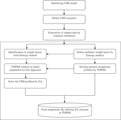
The hybrid GA-TOPSIS-simulation (HGTS) is an extremely efficient approach for selection of the optimum operator allocations in CMS. First, we define the scenarios by considering all available conditions. In this stage, we study the CMS environment. Then, we define significant scenarios based on the number of working shifts and operators. A simulation model is developed and run to identify the efficiency of each scenario. To avoid bias, each scenario is run 30 times. After this stage, we have a data set about all scenarios which shows the value of each criterion. Then, by HGTS, we solve the problem. The steps of HGTS are presented as follows:

1. By the entropy method, we define the weight factor for the each criterion. This step can be ignored if the weight factors are available.

2. In the next step, the procured data from the previous section is used by GA for initialization process.

3. After determining the weight factor, TOPSIS method is used to solve the problem to define the best scenarios.

4. In the fourth step, GA uses the output of TOPSIS as input. In fact, the initial population for GA is the TOPSIS solution.

5. The problem is finally solved by GA and checked by TOPSIS. Moreover, we define the best ranking of scenarios.

The details of how HGTS works in practice are shown in the next section (Section 3). Figure 1 presents the proposed HGTS approach for optimum operator assignment.

Figure 1. The overview of the integrated HGTS approach.

3. Empirical illustration

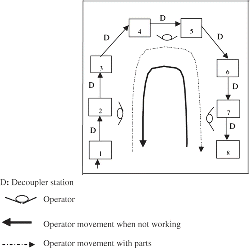
Manned cells are a very flexible system that can adapt to changes in the customer's demand or other changes quite easily and rapidly in the product design. The cells described in this study are designed for flexibility, not line balancing. The walking multi-functional operators permit rapid rebalancing in a U-shaped manner. The considered cell has eight stations and can be operated by one or more operators, depending on the required output for the cell. The times for the operations at the stations do not have to be balanced. The balance is achieved by having the operators walk from station-to-station. The sum of operation times for each operator is approximately equal. In other words, any division of stations that achieves balance between the operators is acceptable. Operators perform scenario movements in cells. Once a production batch size arrives at a cell, it is divided to transfer batch sizes. Transfer batch size is the transfer quantity for intra-cell movements of parts. The ability to rebalance the cell quickly to obtain changes in the output of the cell can be demonstrated by the developed simulation model. The existing manned cell example for a case model is presented in Figure 2 (Azadeh and Anvari 2006).

Figure 2. The existing manned cell example for the case model.

Alternatives for reducing the number of operators in the cell are as follows:

1. Eight operators (one operator for each machine).

2. Seven operators (two operators handling two machines and one operator for each of the rest).

3. Six operators (two operators handling two machines and one operator for each of the rest).

4. Five operators (three operators handling two machines and one operator for each of the rest).

5. Four operators (each operator handling two machines).

6. Six operators (one operator for three machines, others with one machine each).

7. Four operators (one operator handling five machines, three operators with one machine each).

8. Three operators (two operators handling three machines each and one operator handling two machines).

9. Five operators (one operator to four machines and one operator for each of others).

10. Three operators (one operator to four machines and two operators handling two machines each).

11. Three operators (one operator to four machines and one operator to three machines and one operator to one machine).

12. Two operators (one operator for four machines).

In simulation experiments, when the machines are assigned to the operators, the cycle time of the bottleneck resource is chosen as close as possible to the cycle time of the operator. The developed model includes the some assumptions and constraints as follows:

• The self-balancing nature of the labor assignment accounts for differences in operator efficiency.

• The machines have no downtime during the simulated time.

• The time for the operators to move between machines is assumed to be zero. The machines are all close to each other.

• The sum of the multi-function operation times for each operator is approximately equal.

• There is no buffer for the station work.

As mentioned, outputs collected from simulation model are the average lead time of demand, the average of waiting time of demand, average operator and machine utilization, and the number of completed parts per annum. The results of the simulation experiment are used to compare the efficiency of the alternatives. Each labor assignment scenario considers three shifts with 1, 2, or 3 shifts per day. Moreover, a flexible simulation model (Figure 3) is built by Visual SLAM (Pritsker 1995), which incorporates all 36 scenarios for quick response and results. Furthermore, ability to rebalance the cell quickly to obtain changes in output of cell can be demonstrated by the simulation model. So, in the developed model, different demand levels and part types have been taken into consideration.

Figure 3. Simulation model of operators’ allocation in CMS.

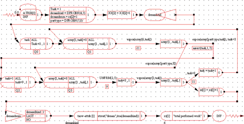
System performance was monitored for different workforce levels and shifts by means of simulation. In simulation experiments, each of the demanded parts had a special type and level. The types of parts that the cell can produce and levels of demand within the cell were determined as two and three by experiment. The time processing of jobs for each of the stations works is related to the part type. The objective of scenarios consists of reducing the number of operators in the cell, and observing how the operation is distributed among the operators. After deletion of transient state, the 36 scenarios were executed for 2000 h (250 working days, each day composed of three shifts, each shift consisting of 8 h of operation). Each scenario was also replicated 30 times to insure that reasonable estimates of means of all outputs could be obtained.

The Table 1 shows the output of the simulation model.

Table 1. Simulation results for the case model (decision matrix).

	X 1	X 2	X 3	X 4	X 5	X 6
Scenarios	Number of operators	Average lead time of demand	Average waiting time of demand	Number of completed parts	Operator utilization	Average machine utilization
Sen1-1	8	303.41	136.35	675	20.19	43.59
Sen1-2	16	251.75	110.21	815	7.65	16.08
Sen1-3	24	213.07	118.69	740	10.80	22.68
Sen2-1	7	269.95	118.80	585	15.77	28.55
Sen2-2	14	232.12	88.63	655	10.20	18.54
Sen2-3	21	220.35	95.50	870	4.03	7.06
Sen3-1	6	267.90	101.12	595	28.90	43.13
Sen3-2	12	231.43	86.08	740	28.38	43.91
Sen3-3	18	213.70	97.71	690	10.00	15.86
Sen4-1	5	305.55	239.57	565	50.85	65.20
Sen4-2	10	245.62	105.61	885	16.71	21.98
Sen4-3	15	227.37	82.83	655	6.81	8.96
Sen5-1	4	281.89	115.80	515	38.55	42.56
Sen5-2	8	255.15	101.38	710	24.38	28.86
Sen5-3	12	230.73	85.77	635	7.99	8.61
Sen6-1	6	284.90	87.99	615	21.73	34.14
Sen6-2	12	247.50	116.91	740	19.98	31.90
Sen6-3	18	225.47	103.73	645	11.48	18.24
Sen7-1	4	333.03	129.15	545	35.89	42.05
Sen7-2	8	261.38	97.55	840	20.51	23.40
Sen7-3	12	242.44	102.74	800	13.99	15.99
Sen8-1	3	329.63	100.47	570	40.65	36.83
Sen8-2	6	258.76	107.42	665	23.60	20.99
Sen8-3	9	246.91	201.60	685	20.85	18.43
Sen9-1	3	389.24	152.93	445	60.25	59.75
Sen9-2	6	343.72	165.53	740	47.70	46.86
Sen9-3	9	305.07	152.91	670	25.35	25.00
Sen10-1	3	337.32	114.61	530	53.45	46.60
Sen10-2	6	299.19	238.46	850	32.20	28.54
Sen10-3	9	263.20	204.81	720	23.45	21.23
Sen11-1	3	363.18	196.82	535	60.20	55.70
Sen11-2	6	276.19	110.25	615	29.15	26.61
Sen11-3	9	261.57	107.71	680	23.25	21.95
Sen12-1	2	361.91	185.12	505	64.88	49.63
Sen12-2	4	329.36	248.24	875	74.33	54.90
Sen12-3	6	291.53	106.71	660	31.13	22.15

3.1. Application of HGTS approach

A total of 36 scenarios were selected as the core of our study. The values of the six indices for the operator assignment are presented in Table 1. The main structure of HGTS in this study is based on the assumption that the best scenario is identified with the indices in which each is the maximum value of its possible values. Therefore, for the scenario 36, a scenario with the best possible attribute, called our goal in the problem, illustrates the maximum present abilities in operator assignment. To achieve the appropriate rank (array), every possible array, comprising 36 scenarios, is considered as a 64-bit chromosome. Then, in accordance with the sequence in the chromosome, the total distance among the first scenario which can be scenario from 1 to 36 and our goal (scenario 36), the second scenario with the first and the next with upper-ranked scenario are calculated.

Respectively, the total distance mentioned above is a variable, dependent on the scenarios’ positions in the array. Consequently, in each chromosome, we can find a new value for total distance. Undoubtedly, the best sequence of the scenarios is an array which has the minimum total distance with high internal cohesion among its scenarios. In fact, our fitness function is a multivariate combination in which its most prominent components are total distance and variance. The above genetic concepts are achieved through a set of well-defined steps as follows:

Step 1

Normalize the index vectors. The six attributes must be normalized and have same order to be used in HGTS. Indices X ₁, X ₂, and X ₃ have opposite order than the rest of the indices.

Step 2

Standardize the indices X ₁− X ₆. The indices are standardized and shown in Table 2. They are standardized through predefined mean and standard deviation for each index.

Table 2. Standardized matrix for the six indices.

Scenarios	Number of operators	Average lead time of demand	Average waiting time of demand	Number of completed parts	Operator utilization	Average machine utilization
Sen1-1	0.184	−0.550	−0.113	0.010	−0.444	0.825
Sen1-2	−1.289	0.560	0.438	1.246	−1.140	−0.979
Sen1-3	−2.762	1.390	0.259	0.584	−0.965	−0.546
Sen2-1	0.368	0.169	0.257	−0.785	−0.689	−0.161
Sen2-2	−0.921	0.981	0.892	−0.167	−0.998	−0.818
Sen2-3	−2.210	1.234	0.747	1.731	−1.341	−1.570
Sen3-1	0.552	0.213	0.629	−0.696	0.039	0.794
Sen3-2	−0.552	0.996	0.946	0.584	0.010	0.846
Sen3-3	−1.657	1.377	0.701	0.142	−1.009	−0.994
Sen4-1	0.737	−0.596	−2.287	−0.961	1.256	2.242
Sen4-2	−0.184	0.691	0.535	1.864	−0.637	−0.592
Sen4-3	−1.105	1.083	1.014	−0.167	−1.186	−1.446
Sen5-1	0.921	−0.087	0.320	−1.403	0.574	0.757
Sen5-2	0.184	0.487	0.624	0.319	−0.212	−0.141
Sen5-3	−0.552	1.011	0.952	−0.343	−1.121	−1.469
Sen6-1	0.552	−0.152	0.906	−0.520	−0.359	0.205
Sen6-2	−0.552	0.651	0.297	0.584	−0.456	0.058
Sen6-3	−1.657	1.124	0.574	−0.255	−0.927	−0.837
Sen7-1	0.921	−1.186	0.039	−1.138	0.426	0.724
Sen7-2	0.184	0.353	0.704	1.467	−0.427	−0.499
Sen7-3	−0.552	0.760	0.595	1.113	−0.788	−0.985
Sen8-1	1.105	−1.113	0.643	−0.917	0.690	0.381
Sen8-2	0.552	0.409	0.496	−0.078	−0.255	−0.657
Sen8-3	0.000	0.664	−1.487	0.098	−0.408	−0.825
Sen9-1	1.105	−2.393	−0.462	−2.021	1.777	1.884
Sen9-2	0.552	−1.415	−0.727	0.584	1.081	1.039
Sen9-3	0.000	−0.585	−0.462	−0.034	−0.158	−0.394
Sen10-1	1.105	−1.278	0.345	−1.270	1.400	1.022
Sen10-2	0.552	−0.459	−2.263	1.555	0.222	−0.162
Sen10-3	0.000	0.314	−1.555	0.407	−0.263	−0.641
Sen11-1	1.105	−1.833	−1.386	−1.226	1.775	1.619
Sen11-2	0.552	0.035	0.437	−0.520	0.053	−0.289
Sen11-3	0.000	0.349	0.490	0.054	−0.275	−0.594
Sen12-1	1.289	−1.806	−1.140	−1.491	2.034	1.221
Sen12-2	0.921	−1.107	−2.469	1.775	2.558	1.566
Sen12-3	0.552	−0.294	0.511	−0.123	0.162	−0.581

Step 3

Define the production module. This module is defined to create and manipulate the 50-individual population by filling it with randomly generated individuals. Each individual is defined by a 64-bit string.

Step 4

Define recombination module which comprises four sections:

• Tournament selection operator chooses individuals with probability 80% from the population for reproduction.

This is considered a popular type of selection method in HGTS. The basic concept in a tournament is that the best string in the population will win both its tournaments, while the worst will never win, and thus will never be selected. However, in this study, the other kinds of selection methods named sigma scaling and rank selection are considered in order to determine the best method.

• Uniform crossover operator which combines bits from the selected parents with the probability of 85%.

• Mutation operator consists of making (usually small) alterations to the values of one or more genes in a chromosome.

• Regeneration operator which is used to create 100-individual generations.

Step 5

Define evaluation module:

The fitness function to determine the goodness of each individual based on the objectives is defined by the total distance and variance that can be shown by

where i is the number of scenarios (DMUs) and j the number of criteria.

In the above-mentioned formula, d _Total indicates the total distance between adjacent scenarios.

The evaluation of operator assignment is the ability of each chromosome to satisfy the objective function. Therefore, our motivation to obtain the best array in this problem is to minimize the fitness function mentioned above. After producing 1000 generations, we reach the best fitness function value, 295.362, related to the chromosome which can be shown by the sequence at Table 3.

Table 3. Simulation results for the case model (decision matrix).

	X 1	X 2	X 3	X 4	X 5	X 6
Scenarios	Number of operators	Average lead time of demand	Average waiting time of demand	Number of completed parts	Operator utilization	Average machine utilization
Sen1-1	8	303.41	136.35	675	20.19	43.59
Sen1-2	16	251.75	110.21	815	7.65	16.08
Sen1-3	24	213.07	118.69	740	10.80	22.68
Sen2-1	7	269.95	118.80	585	15.77	28.55
Sen2-2	14	232.12	88.63	655	10.20	18.54
Sen2-3	21	220.35	95.50	870	4.03	7.06
Sen3-1	6	267.90	101.12	595	28.90	43.13
Sen3-2	12	231.43	86.08	740	28.38	43.91
Sen3-3	18	213.70	97.71	690	10.00	15.86
Sen4-1	5	305.55	239.57	565	50.85	65.20
Sen4-2	10	245.62	105.61	885	16.71	21.98
Sen4-3	15	227.37	82.83	655	6.81	8.96
Sen5-1	4	281.89	115.80	515	38.55	42.56
Sen5-2	8	255.15	101.38	710	24.38	28.86
Sen5-3	12	230.73	85.77	635	7.99	8.61
Sen6-1	6	284.90	87.99	615	21.73	34.14
Sen6-2	12	247.50	116.91	740	19.98	31.90
Sen6-3	18	225.47	103.73	645	11.48	18.24
Sen7-1	4	333.03	129.15	545	35.89	42.05
Sen7-2	8	261.38	97.55	840	20.51	23.40
Sen7-3	12	242.44	102.74	800	13.99	15.99
Sen8-1	3	329.63	100.47	570	40.65	36.83
Sen8-2	6	258.76	107.42	665	23.60	20.99
Sen8-3	9	246.91	201.60	685	20.85	18.43
Sen9-1	3	389.24	152.93	445	60.25	59.75
Sen9-2	6	343.72	165.53	740	47.70	46.86
Sen9-3	9	305.07	152.91	670	25.35	25.00
Sen10-1	3	337.32	114.61	530	53.45	46.60
Sen10-2	6	299.19	238.46	850	32.20	28.54
Sen10-3	9	263.20	204.81	720	23.45	21.23
Sen11-1	3	363.18	196.82	535	60.20	55.70
Sen11-2	6	276.19	110.25	615	29.15	26.61
Sen11-3	9	261.57	107.71	680	23.25	21.95
Sen12-1	2	361.91	185.12	505	64.88	49.63
Sen12-2	4	329.36	248.24	875	74.33	54.90
Sen12-3	6	291.53	106.71	660	31.13	22.15

3.2. Implementation of TOPSIS

For the first step of this methodology, the decision matrix (Table 1), representing the performance values of each alternative with respect to each criterion, is computed by a simulation model. Next, these performance values are normalized by Equation 2. In Step 3, the normalized matrix is multiplied with the criteria weights calculated by the entropy method (Table 4). The step of defining the ideal solution consists of taking the best values of alternatives and using similar principles, obtaining the negative-ideal solution by taking the worst values of alternatives. Subsequently, the alternatives are ranked with respect to their relative closeness to the ideal solution (Table 5).

Table 4. Entropy-weighted coefficients.

Attribute	Index	Dj	Weight
Number of operator	W 1	0.046273	0.296356
Average lead time of demand	W 2	0.003721	0.023834
Average waiting time of demand	W 3	0.016075	0.102952
Number of completed parts	W 4	0.003838	0.024582
Operator utilization	W 5	0.05315	0.340401
Average machine utilization	W 6	0.033082	0.211876

Table 5. The rankings of HGTS versus TOPSIS.

TOPSIS solution				HGTS solution
Scenario	Rank	Scenario	Rank	Scenario	Rank	Scenario	Rank
35	1	8	19	31	1	8	19
34	2	27	20	35	2	27	20
25	3	20	21	25	3	30	21
31	4	4	22	34	4	24	22
28	5	33	23	28	5	33	23
10	6	30	24	10	6	20	24
26	7	24	25	26	7	11	25
22	8	11	26	19	8	4	26
13	9	17	27	13	9	17	27
19	10	21	28	22	10	21	28
7	11	15	29	7	11	15	29
29	12	5	30	23	12	5	30
36	13	12	31	36	13	12	31
32	14	2	32	32	14	2	32
16	15	18	33	16	15	18	33
23	16	9	34	29	16	9	34
14	17	3	35	14	17	3	35
1	18	6	36	1	18	6	36
Score	303.406			Score	295.362

4. Results and discussion

According to the above results, scenario 12-2 (one operator for four machines, two shifts per day) is the most efficient one. The second best scenario is the scenario 12-1, which is similar to scenario 12-2 only with one shift per day. The third best scenario is 9-1 with five operators (one operator for four machines and one operator per machine for the rest with one shift per day). Table 5 presents the rankings of the proposed HGTS versus TOPSIS for the best 18 rankings.

4.1. Verification and validation

DEA and principal component analysis (PCA) are used to verify and validate the results of the proposed HGTS. DEA and PCA are among the most powerful tools in multivariate analysis. However, we show that the proposed algorithm has several advantages over these methods. These are discussed in the following sections. First, mathematical models of DEA and PCA are discussed and their efficiency scores and ranking are evaluated. Then, their ranking scores together with TOPSIS are compared with the proposed HGTS.

4.1.1. Data envelopment analysis

The two basic DEA models are CCR based on Charnes, Cooper and Rhodes (Charnes et al. 1978) and BCC based on Banker, Charnes and Cooper (Banker et al. 1984) with constant returns to scale and variable returns to scale, respectively. DMU_o is assigned the highest possible efficiency score θ_o  ≤ 1 that constraints allow from the available data by choosing the optimal weights for the output and inputs. If DMU_o receives the maximal value θ_o  = 1, then it is efficient, but if θ_o  < 1, it is inefficient, since with its optimal weights, another DMU receives the maximal efficiency. Basically, the model divides the DMUs into two groups, efficient (θ_o  = 1) and inefficient (θ_o  < 1), by identifying the efficient in the data. The original DEA model is not capable of ranking efficient units and therefore it is modified to rank efficient units (Andersen and Petersen 1993).

The original fractional CCR model (14) evaluates the relative efficiencies of 36 scenarios (j = 1, … , 36), each with 3 inputs (average lead-time of demands, average waiting time of demands and the number of the operators (in a working day) and 3 outputs (average operator/machine utilization and numbers of completed parts per year) denoted by x _{1 j} , x _{2 j} , x _{3 j} , y _{1 j} , and y _{2 j} and y _{3 j} , respectively. This is done by maximizing the ratio of weighted sum of output to the weighted sum of inputs:

In model (14), the efficiency of DMU_o is θ _o and u_r and v_i are the factor weights. However, for computational convenience, the fractional programming model (14) is re-expressed in linear program (LP) form as follows:

where ε is a non-Archimedean infinitesimal introduced to insure that all the factor weights have positive values in the solution. The model (16) evaluates the relative efficiencies of 36 scenarios (j = 1, … , 36), respectively, by minimizing inputs (average lead-time of demands, average waiting time of demands, and the number of operators (in a working day) when inputs are constant. The dual of LP model for input-oriented CCR is given as follows:

The output-oriented CCR model is given as follows:

If ∑λ_j  = 1 (j = 1, … , 36) is added to model (16), the BCC model is obtained which is input oriented and its return to scale is variable:

The output-oriented BCC model is shown in Equation (18).

However, the LP model (16) does not allow for ranking of efficient units as it assigns a common index of one to all the efficient scenarios in the data set. Therefore, the dual model (16) was modified by Andersen and Petersen for DEA-based ranking purposes, as follows (Andersen and Petersen 1993):

Model (20), which excludes DMU_o, is under evaluation from the input–output constraints so that the efficient units are assigned an index of greater than one and the index for inefficient units is identical to that of model (3). Model (20) is used to determine the DEA ranking in this article. An insufficient number of scenarios for a DEA model would tend to rate all DMUs 100% efficient, because of an inadequate number of degrees of freedom. A proper scenario number is required for identifying a true performance frontier. A rule of thumb for maintaining an adequate number of degrees of freedom when using DEA is to obtain at least two DMUs for each input or output measure. The results from solving the DEA would generate those performance frontiers that then become the final candidate designs.

4.1.2. Principle component analysis

The objective of PCA is to identify a new set of variables such that each new variable, called a principal component, is a linear combination of original variables. Second, the first new variable y ₁ accounts for the maximum variance in the sample data and so on. Third, the new variables (principal components) are uncorrelated. PCA is performed by identifying the eigenstructure of the covariance or the singular value decomposition of the original data.

Here, the former approach will be discussed. It is assumed that there are 9 variables (indexes) and 36 DMUs, and d_jir  = y_rj /x_ij (i = 1, … ,3; r = l, … ,3) represents the ratios of individual output (average operator/machine utilization and numbers of completed parts per year) to individual input (average lead-time of demands, average waiting time of demands, and the number of the operators (in a working day)) for each DMU _j (j = l, … , 36). Obviously, the bigger the d_jir , the better the performance of DMU _j in terms of the rth output and the ith input. Now let d_jk  = d_jir , where k = 1, … , 9 and 9 = 3 × 3. We need to find some weights that combine those nine individual ratios of d_i for DMU _j . Consider the following 36 × 9 data matrix composed by d_jk : D = (d _l, … , d ₅)_36×9 with each row representing nine individual ratios of d_i for each DMU and each column representing a specific output/input ratio. That is, d_k  = (d_{k 1}, … , d_{k 36})^T. The PCA is employed here to find new independent measures (principal components) which are, respectively, different linear combinations of d _l, … , d ₉ so that the principal components can be combined by their eigenvalues to obtain a weighted measure of d_jk . The PCA process of D is carried out as follows:

Step 1

Calculate the sample mean vector đ and covariance matrix S .

Step 2

Calculate the sample correlation matrix R.

Step 3

Solve the following equation.

We obtain the ordered p characteristic roots (eigenvalues) λ ₁ ≥ λ ₂ ≥ ··· ≥ λ ₉ with ∑λ_j  = 9 (j = 1, … , 9) and the related p characteristic vectors (eigenvectors) (l_{m 1}, l_{m 2} … , l_{m 9}) (m = 1, … , 9). Those characteristic vectors compose the principal components Y_i . The components in eigenvectors are, respectively, the coefficients in each corresponding Y_i :

Step 4

Calculate the weights (w_i ) of the principal components and PCA scores (z_i ) of each DMU (i = 1, … , 36). Furthermore, the z vector (z ₁, … , z ₉) where z_j shows the score of jth DMUs is given by

The DEA and PCA methods are applied to the data set of 36 DMUs. The DEA results show that 12 out of the 36 DMUs are relatively efficient. However, exact ranking cannot be obtained for these DMUs. In order to improve the discriminating power of DEA, the Andersen and Petersen (1993) model was utilized. Also, PCA rankings of 36 DMUs with respect to 9 indicators (output/input) were obtained. DEA efficiency scores and PCA scores together with rankings of DMUs are shown in Table 6.

Table 6. Results of DEA and PCA for 36 labor-assignment scenarios.

Scenario	DEA score	DEA rank	Z pca	PCA rank
Sen1-1	0.88	25	0.137262	14
Sen1-2	0.87	27	−1.93488	33
Sen1-3	0.97	16	−0.42223	18
Sen2-1	0.78	35	−1.59225	30
Sen2-2	0.84	30	−1.40223	28
Sen2-3	0.92	18	−1.22056	26
Sen3-1	1.03	11	1.131111	10
Sen3-2	1.32	3	1.717474	7
Sen3-3	0.87	26	−2.13083	35
Sen4-1	1.26	4	2.613937	4
Sen4-2	0.86	28	−2.79368	36
Sen4-3	0.88	24	−1.77313	32
Sen5-1	0.98	14	0.80638	12
Sen5-2	0.93	17	−0.19444	17
Sen5-3	0.84	29	−2.01194	34
Sen6-1	1.01	12	0.51764	13
Sen6-2	0.88	23	−0.58377	21
Sen6-3	0.79	34	−1.52258	29
Sen7-1	0.89	22	−0.73232	23
Sen7-2	1.10	8	1.36003	9
Sen7-3	0.91	21	−1.62194	31
Sen8-1	1.16	6	2.035429	6
Sen8-2	0.92	19	−0.46171	19
Sen8-3	0.82	32	−1.33913	27
Sen9-1	1.12	7	3.171607	2
Sen9-2	1.10	9	0.946035	11
Sen9-3	0.69	36	−0.7505	24
Sen10-1	1.17	5	2.964201	3
Sen10-2	0.97	15	−0.50993	20
Sen10-3	0.82	33	−1.18616	25
Sen11-1	0.99	13	1.652479	8
Sen11-2	1.08	10	0.059721	15
Sen11-3	0.83	31	−0.7177	22
Sen12-1	1.62	1	3.735966	1
Sen12-2	1.42	2	2.161883	5
Sen12-3	0.91	20	−0.10925	16

4.1.3. Correlation analysis

Table 7 shows a correlation between HGTS and other methods, namely, DEA and principal component analysis (PCA). Table 7 also reports the results of nonparametric statistical tests of the relationship between the stated techniques which result in the rejection of H ₀ at 0.01 levels.There is a high correlation between HGTS and TOPSIS. Also, correlation between HGTS and PCA is very high (0.809), which shows that HGTS results are reasonable. Spearman's rho correlations comparing these methods imply that results of all methods except DEA are not statistically different. Thus, there is a direct relationship between HGTS, DEA, PCA, and TOPSIS in terms of data sets generated by computer simulation with respect to the 36 scenarios. Particularly, the Spearman test statistic r_s  > 0.75 indicates a strong direct relationship. Also, we apply analysis of variance (ANOVA) to show if the proposed approach produces greater efficiency scores than DEA, PCA, and TOPSIS.

Table 7. Non-parametric Spearman (r_s ) correlations analysis.

	HGTS	DEA	PCA
TOPSIS	0.987	0.574	0.833
HGTS		0.542	0.809
DEA			0.728

Table 8. ANOVA results of HGTS versus other methods.

Source	DF	Sum of squares	Mean square	F	p-value
Block	3	243.972	81.324	112.08	0.000
Treatment	35	80.65	2.3044	3.18	0.000
Error	105	76.18	0.7256
Total	143	400.8147

4.1.4. Analysis of variance

ANOVA was used to evaluate the effects of the optimum operator assignment in CMS model. DMU's efficiencies were considered for HGTS model in comparison with DEA, PCA, and TOPSIS methods. First, it was tested whether efficiencies have the same behavior in HGTS (τ ₁), DEA (τ ₂), PCA (τ ₃), and TOPSIS (τ ₄) models. Furthermore, it is tested whether the null hypothesis H ₀: μ ₁= μ ₂= μ ₃= μ ₄ was to be accepted. It was concluded that the four treatments differ at α = 0.05. Furthermore, the least significant difference (LSD) method is used to compare the pairs of treatment means μ ₁, μ ₂, μ ₃ and μ ₄. That is H ₀: μ_i  = μ_j for all . The results of LSD revealed that at α = 0.05, μ ₁> μ ₂, μ ₃, μ ₄ and μ ₂> μ ₃, μ ₄ also μ ₃= μ ₄ and hence treatment 1 (HGTS) produces a significantly greater efficiency than other treatments. The advantages of the HGTS model with respect to efficiencies are shown in Tables 8 and 9.

Table 9. Multiple comparisons between HGTS and other methods.

	(I) VAR00001	(J) VAR00001	Mean difference (I−J) Lower bound	Standard error Upper bound	Significance Lower bound	95% confidence interval
Upper bound						Lower bound
LSD	HGTS	DEA	2.40335(*)	0.24957	0.000	1.9099	2.8968
		PCA	3.38752(*)	0.24957	0.000	2.8941	3.8809
		TOPSIS	2.89899(*)	0.24957	0.000	2.4056	3.3924
	DEA	HGTS	−2.40335(*)	0.24957	0.000	−2.8968	−1.9099
		PCA	0.98417(*)	0.24957	0.000	0.4907	1.4776
		TOPSIS	0.49564(*)	0.24957	0.049	0.0022	0.9891
	PCA	HGTS	−3.38752(*)	0.24957	0.000	−3.8809	−2.8941
		DEA	−0.98417(*)	0.24957	0.000	−1.4776	−0.4907
		TOPSIS	−0.48853	0.24957	0.052	−0.9820	0.0049
	TOPSIS	HGTS	−2.89899(*)	0.24957	0.000	−3.3924	−2.4056
		DEA	−0.49564(*)	0.24957	0.049	−0.9891	−0.0022
		PCA	0.48853	0.24957	0.052	−0.0049	0.9820
Note: *The mean difference is significant at the 0.05 level.

4.1.5. Qualitative comparison

We have proved that the proposed approach of this study provides good correlation with other robust multivariate methods. We have also shown that HGTS provides higher efficiency scores than previous methods through ANOVA and LSD. A comparative study between HGTS and other methods is presented in Table 10. All methods can solve problems with multiple inputs and outputs, but HGTS can locate the best DMU with both specified and unspecified priori weights. Clearly, the hybrid model is capable of solving decision-making models with great flexibility and it consequently demonstrates efficient ranking of alternatives.

Table 10. Distinct features of HGTS versus other methods.

	Multiple inputs	Multiple outputs	No need for prior assignment of weights	Ranking capability	Specification of weights for each indicator	Flexibility on the basis of assigning weights
TOPSIS	√	√	–	√	√	–
HGTS	√	√	√	√	√	√
PCA	√	√	√	√	–	–
DEA	√	√	√	√	–	–

5. Conclusion

This article presented a decision-making approach based on a HGTS for determining the most efficient number of operators and the efficient measurement of operator assignment in CMS. The objective was to determine the labor assignment in a CMS environment with the optimum performance. We used HGTS for obtaining near optimum ranking of the alternative in accordance with fitness function. Also, this approach was performed by employing the number of operators, average lead time of demand, average waiting time of demand, number of completed parts, operator utilization, and average machine utilization as attributes. Entropy method was used to determine the weight of attributes. Furthermore, values of the attributes were procured by means of computer simulation. The unique feature of this model is demonstration of efficient ranks of alternatives by reducing the distance between neighborhood alternatives. The superiority and advantages of the proposed HGTS were shown through a comparative study composed by TOPSIS, DEA, and PCA.

HGTS used was introduced as a powerful method for ranking the scenarios in the operator assignment problem based on the attributes discussed in this article. Also, the TOPSIS approaches verified our findings. But TOPSIS is not able to present efficient ranking of scenarios for complicated problems. Furthermore, the HGTS approach is capable of ranking the alternatives by near optimum fitness function and it determines the best solution with minimum distance.

The decision matrix is introduced for selecting the appropriate scenario for the operator assignment in CMS. The weighted coefficients are obtained for every attribute by making use of the entropy method. The decision matrix and weighted coefficients are taken as the inputs for ordinary TOPSIS. These models list candidate scenarios from the best to the worst, taking into account all scenario selection criteria including attributes. Methods that determine both the score and the rank of each candidate scenario may be preferred over methods that provide only the ranks of scenarios. The score option can provide better insight for designers and it takes into account both the differences and similarities of the candidate scenarios. HGTS can be considered an efficient tool to enhance the accuracy of the final decision in designing a CMS system, as we have shown in this article.

Nomenclature

Ci	=	the relative closeness of ith candidate material to the ideal solutions
Ej	=	the entropy value for jth attribute
J	=	the set of decision attributes
k	=	constant of the entropy equation
K	=	set of benefit criteria
K′	=	set of cost criteria
m	=	the number of scenarios
n	=	the number of criteria
nij	=	an element of the normalized decision matrix
pij	=	an element of the decision matrix in the normalized mode for entropy method
rij	=	an element of the decision matrix
	=	the best value of jth attribute
	=	the worst value of jth attribute
	=	distance of design to the ideal solution for the ith candidate material
	=	distance of design from the negative ideal solution for the ith candidate
s	=	the number of outputs
V	=	weighted normalized decision matrix
Vij	=	an element of the weighted normalized decision matrix
	=	ideal solution for jth attribute
	=	negative ideal solution for jth attribute
vi	=	the weight given to input i
	=	the weight coefficient of jth attribute
wj	=	balanced weight coefficient of jth attribute
X	=	the vector of optimization variables
Xj	=	jth attribute in the decision matrix
Xij	=	the amount of input i produced by unit j
Yrj	=	the amount of output r produced by unit j
μr	=	The weight given to output r
λ j	=	the priority of jth attribute comparing with others
θ jo	=	the efficiency score of DMU0
ε	=	a non-Archimedean infinitesimal

References

- Anderson , P. and Peterson , N.C. 1993 . A procedure for ranking efficient units in data envelopment analysis . Management Science , 39 ( 10 ) : 1261 – 1264 .
- Askin , R and Huang , Y . 2001 . Forming effective worker teams for cellular manufacturing . International journal of production research , 39 ( 11 ) : 2431 – 2451 .
- Ayag , Z and Ozdemir , RG . 2006 . A fuzzy AHP approach to evaluating machine tool alternatives . Journal of intelligent manufacturing , 17 ( 2 ) : 179 – 190 .
- Azadeh , A and Anvari , M . 2006 . Implementation of multivariate methods as decision making models for optimization of operator allocation by computer simulation in CMS . In: Proceedings of the 2006 summer computer simulation conference . 2006 , Calgary, Canada. pp. 34 – 41 .
- Banker , RD , Charnes , A and Cooper , WW . 1984 . Some models for estimating technical and scale inefficiencies in data envelopment analysis . Management science , 30 ( 9 ) : 1078 – 1092 .
- Bidanda , B . 2005 . Human related issues in manufacturing cell design, implementation, and operation: a review and survey . Computers and industrial engineering , 48 ( 3 ) : 507 – 523 .
- Camanho , AS and Dyson , RG . 2005 . Cost efficiency measurement with price uncertainty: a DEA application to bank branch assessments . European journal of operational research , 161 ( 2 ) : 432 – 446 .
- Cesani , VI and Steudel , HJ . 2005 . A study of labour assignment flexibility in cellular manufacturing systems . Computers and industrial engineering , 48 ( 3 ) : 571 – 591 .
- Charnes , A , Cooper , WW and Rhodes , E . 1978 . Measuring the efficiency of decision making units . European journal of operational research , 2 ( 6 ) : 429 – 444 .
- Chauvet , F , Proth , JM and Soumare , A . 2000 . The simple and multiple job assignment problems . International journal of production research , 38 ( 14 ) : 3165 – 3179 .
- Doyle , J and Green , R . 1994 . Efficiency and cross-efficiency in DEA: derivations, meanings and uses . Journal of the operational research society , 45 ( 5 ) : 567 – 578 .
- Ebrahimipour , V . 2007 . A GA–PCA approach for power sector performance ranking based on machine productivity . Applied mathematics and computation , 186 ( 2 ) : 1205 – 1215 .
- Edirisinghe , NCP and Zhang , X . 2007 . Generalized DEA model of fundamental analysis and its application to portfolio optimization . Journal of banking & finance , 31 ( 11 ) : 3311 – 3335 .
- Ertay , T . 2002 . An analytical approach to technology selection problem: a case study in plastic mold production . International journal of operations and quantitative management , 8 ( 3 ) : 165 – 179 .
- Ertay , T and Ruan , D . 2005 . Data envelopment analysis based decision model for optimal operator allocation in CMS . European journal of operational research , 164 ( 3 ) : 800 – 810 .
- Fitzpatrick , E and Askin , R . 2005 . Forming effective worker teams with multi-functional skill requirements . Computers and industrial engineering , 48 ( 3 ) : 593 – 608 .
- Haupt , SE and Haupt , RL . 1998 . Practical genetic algorithm, , 2nd , New York, NY : John Wiley .
- Hsu-Shih , S . 2008 . Incremental analysis for MCDM with an application to group TOPSIS . European journal of operational research , 186 ( 2 ) : 720 – 734 .
- Hwang , CL and Yoon , K . 1981 . Multiple attributes decision making methods and applications , Berlin, Germany : Springer .
- Jeff , KS , Aleda , VR and Wendell , GG . 2001 . The deployment of temporary production workers in assembly operations: a case study of the hidden costs of learning and forgetting . Journal of operation management , 21 ( 6 ) : 689 – 707 .
- Liu , ST . 2008 . A fuzzy DEA/AR approach to the selection of flexible manufacturing systems . Computers and industrial engineering , 54 ( 1 ) : 66 – 76 .
- Mannino , M , Hong , SN and Choi , IJ . 2008 . Efficiency evaluation of data warehouse operations . Decision support systems , 44 ( 4 ) : 883 – 898 .
- Molleman , E and Slomp , J . 1999 . Functional flexibility and team performance . International journal of production research , 37 ( 8 ) : 1837 – 1858 .
- Nembhard , DA . 2001a . An empirical comparison of forgetting model . IEEE transactions on engineering management , 48 ( 3 ) : 283 – 291 .
- Nembhard , DA . 2001b . Heuristic approach for assigning workers to tasks based on individual learning rates . International journal of production research , 39 ( 9 ) : 1955 – 1968 .
- Nembhard , DA and Mustafa , VU . 2000 . Experiential learning and forgetting for manual and cognitive tasks . International journal of industrial ergonomics , 25 ( 4 ) : 315 – 326 .
- Olson , DL . 2004 . Comparison of weights in TOPSIS models . Mathematical and computer modeling , 40 ( 7–8 ) : 721 – 727 .
- Önüt , S , Soner Kara , S and Efendigil , T . 2008 . A hybrid fuzzy MCDM approach to machine tool selection . Journal of intelligent manufacturing , 19 ( 4 ) : 443 – 453 .
- Pritsker , AAB . 1995 . Introduction to simulation and SLAM II, , 4th , New York, NY : John Wiley and System Publishing Corporation .
- Rao , RV . 2006 . A material selection model using graph theory and matrix approach . Material science engineering , 43 ( 1–2 ) : 248 – 255 .
- Roy , B . 1991 . The outranking approach and the foundations of ELECTRE methods . Theory and decision , 31 ( 1 ) : 49 – 73 .
- Roy , B . 1996. Multicriteria methodology for decision aiding. Vol. 12 of non-convex optimization and its applications. Dordrecht, Netherlands: Kluwer Academic Publishers
- Saaty , TL . 1990 . Decision making for leaders, the analytical hierarchy process for decision in a complex world , Pittsburgh, PA : RWS Publications .
- Saaty , TL . 2000 . Fundamentals of decision making and priority theory with the analytic hierarchy process , Pittsburgh, PA : RWS Publications, University of Pittsburgh .
- Sarkis , J and Talluri , S . 1998 . A decision model for evaluation of flexible manufacturing systems in the presence of both cardinal and ordinal factors . International journal of production research , 37 ( 13 ) : 2927 – 2938 .
- Scott , MS , Nembhard , DA and Mustafa , VU . 2001 . The effects of worker learning, forgetting, and heterogeneity on assembly line productivity . Management science , 47 ( 12 ) : 1639 – 1653 .
- Shanian , A and Savadogo , O . 2006 . TOPSIS multiple-criteria decision support analysis for material selection of metallic bipolar plates for polymer electrolyte fuel cell . Journal of power sources , 159 ( 2 ) : 1095 – 1104 .
- Simos , J and Gestion , J . 1990. D′echets solides urbains Genevois: les faits, le traitement, l’analyse. Presses Polytechniques et Universitaires Romandes, Lausanne, Switzerland
- Slomp , J , Bokhorst , J and Molleman , E . 2005 . Cross training in a cellular manufacturing environment . Computer and industrial engineering , 48 ( 3 ) : 609 – 624 .
- Slomp , J and Molleman , E . 2000 . Cross training policies and performance of teams . Proceedings of the group technology/cellular manufacturing world symposium 2000. San Juan . 2000 , Puerto Rico. pp. 107 – 112 .
- Süer , GA and Tummaluri , RR . 2008 . Multi-period operator assignment considering skills, learning and forgetting in labour-intensive cells . International journal of production research , 46 ( 2 ) : 469 – 493 .
- Wittrock , RJ . 1992 . Operator assignment and the parametric preflow algorithm . Management science , 38 ( 9 ) : 1354 – 1359 .
- Yang , T , Chen , M-C and Hung , C-C . 2007 . Multiple attribute decision-making methods for the dynamic operator allocation problem . Mathematics and computers in simulation , 73 ( 5 ) : 285 – 299 .
- Zhang , H , Gen , M and Seo , Y . 2006 . An effective coding approach for multiobjective integrated resource selection and operation sequences problem . Journal of intelligent manufacturing , 17 ( 4 ) : 385 – 397 .