Genotype × environment interactions and yield stability of stress-tolerant open-pollinated maize varieties in the Eastern Cape province, South Africa

Abstract

Genotype × environment interactions are inherent in multilocational trials and complicate identification of superior genotypes. The aim of the study was to determine yield performance and stability of 13 maize genotypes in five locations of the Eastern Cape province, South Africa. The genotypes assessed were: ZM305, ZM423, ZM501, ZM525, ZM621, ZM627 and Obatanpa from the International Maize and Wheat Improvement Centre; BR993 and COMP4 from the International Institute of Tropical Agriculture; four local checks, AFRIC 1, Okavango, Nelson's Choice, and PAN 6479. Yield data were subjected to analysis of variance (ANOVA) and additive main effects and multiplicative interaction (AMMI) analysis. According to ANOVA, genotype × environment interaction was significant. PAN 6479 (5.21 t ha^-1) and ZM525 (5.19 t ha^-1) were the highest-yielding varieties, whereas Okavango (4.08 t ha^-1) showed the lowest yield. Based on AMMI analysis, BR993 and Obatanpa were the least stable genotypes. PAN 6479 and ZM525 showed specific adaptations to high potential environments. Obatanpa was adapted to environments with low-yielding potential, since improvement of the environment did not improve its yield. ZM501 was the most stable genotype, and showed no significant yield difference to PAN 6479. ZM501 can therefore be assigned to several environments in the Eastern Cape.

Keywords:

• additive main effects and multiplicative interaction
• AMMI stability values
• genotype × environment interaction
• yield stability

Introduction

Maize is an important cereal crop grown by most resource-poor farmers in the Eastern Cape (EC) province of South Africa (Bembridge 2000). Yields achieved by these farmers are low, ranging from less than 1 t ha^-1 in rain-fed production systems to less than 3 t ha^-1 under irrigation (Fanadzo et al. 2010), making it difficult to achieve provincial targets of self-sufficiency to feed a growing rural population of 4.5 million.

There are a number of socioeconomic constraints that characterise maize production in the EC, such as lack of capital, lack of technical know-how, low availability of labour and old age (Fraser et al. 2003). Abiotic and biotic constraints, for instance, low soil fertility, pests and diseases, and use of inappropriate maize varieties also play a role in limiting the productivity of maize (Bembridge 2000). The use of hybrids and production packages recommended by the Eastern Cape Department of Agriculture in irrigation schemes such as Keiskammahoek, Tyhefu and Zanyokwe, and in agricultural cooperatives across the EC, has resulted in high production costs and reduced viability at yield levels achieved by small-scale farmers (Fanadzo et al. 2010). As a result, many farmers have been left with high levels of debt on agricultural loans, and increased vulnerability to food insecurity and reduced rural livelihoods (MEDPT 2010). The suggestion that farmers may be using inappropriate varieties in the EC (Fanadzo et al. 2010; MEDPT 2010) provided an entry point for testing of stress-tolerant open-pollinated varieties (OPVs) of maize as alternatives for resource-poor farmers.

As a way of improving maize production by resource-poor farmers located in marginal areas, the International Maize and Wheat Improvement Centre (CIMMYT) and International Institute of Tropical Agriculture (IITA) continuously develop a range of stress-tolerant OPVs of maize (Pixley and Bänziger 2004; Bänziger et al. 2005; Setimela et al. 2007). Research has shown that these varieties have conferred either specific or wide adaptation to different environments in countries such as Malawi, Zambia (Bänziger et al. 2005), Zimbabwe (Gadzirayi et al. 2006) and in selected districts of South Africa (Mkhari et al. 2006). Furthermore, their use has led to significant improvements of maize yields and farmer livelihoods (Gadzirayi et al. 2006; Mkhari et al. 2006). Introduction of these low cost, highly adaptable and stress-tolerant varieties could, therefore, help farmers in the EC increase maize productivity. In turn, this could lead to improved rural livelihoods and alleviation of poverty. However, the adaptation and yield performance of these varieties must be tested in the EC. In addition, much attention has to be given to the study of the effect of genotype × environment interaction (GEI) on variety stability, because these are factors that could affect variety recommendations to different target sites in the province.

Inconsistent genotypic responses to environmental factors such as temperature, soil moisture, and soil type or fertility level from location to location and year to year are a function of GEI (Ceccarelli et al. 1994). This phenomenon has also been mentioned in numerous reports as a cause of genetic instability and poor performance of some high-yielding varieties (Muungani et al. 2007; Setimela et al. 2007; Admassu et al. 2008; Asfaw et al. 2009). Therefore, GEI is commonly considered by plant breeders and researchers as one of the main factors influencing effective variety recommendations (Muungani et al. 2007). As a result, analysis of its contribution in multilocational trials becomes important when evaluating diverse varieties (Yan et al. 2007).

Before recommending suitable varieties for resource-poor farmers living in diverse agroecologies of the EC, it is essential that the contribution of GEI on prospective varieties is understood. According to Kang et al. (2004), a variety could be high yielding and show a low degree of rank fluctuation when grown over diverse environments and seasons, thus, displaying broad adaptation and good yield stability (low GEI). Furthermore, varieties could also show specific adaptations, that is, giving high yields in selected environments over seasons, thus providing significant advantages in particular environments (large GEI) (Kang et al. 2004). This implies that, if a range of varieties is to be tested in contrasting environments, varieties showing wide or specific adaptations should be identified.

A combined analysis of variance (ANOVA) can be used to quantify GEI and describe the main effect. However, ANOVA does not fully explain the interaction between the genotypes and environments (Admassu et al. 2008), thus failing to distinguish varieties that exhibit specific or wide adaptation. To explain the interaction of the main effects beyond ANOVA, other statistical models can be employed. One such model is the additive main effects and multiplicative interaction model (AMMI) proposed by Zobel et al. (1988). Ma'ali (2008) showed its usefulness in identifying stable varieties that had been tested across eastern and western maize-growing regions in South Africa. Asfaw et al. (2009) used it to identify the extent of specific variety–environment interactions in Ethiopia, while Mohammadi et al. (2007) used it to identify wheat varieties that had specific adaptations in specific environments in Iran. Furthermore, Yan et al. (2007) also showed the usefulness of biplots generated by the AMMI model in evaluation and identification of mega-environments and test environments.

The AMMI model has been shown to be effective in understanding GEI, as well as increasing the precision of making variety recommendations to different target sites, and evaluating test environments. Therefore, the objective of the study was to determine the yield performance and stability of maize varieties grown over three seasons across selected environments in the EC.

Materials and methods

Site selection and description

The study was conducted in three consecutive summer seasons, namely, 2009/2010, 2010/2011 and 2011/2012, in selected environments of the EC. The sites were purposefully selected according to their heterogeneity, in terms of geographic location, altitude, soil characteristics and rainfall (see Tables 1 and 2). Trials were established at five sites: Mqekezweni, Mkhwezo, Jixini, Qxididi and Gogozayo. During the 2009/2010 and 2010/2011 seasons, trials at Qxididi and Jixini, respectively, did not establish due to low rainfall and these do not appear in the combined analysis, but were included when determining genotype and environmental stability. Table 3 refers to code names assigned to environments (sites within seasons) used in the stability analysis.

Table 1: Description of the experimental sites based on geoclimatic data

Site	Site code	Latitude	Longitude	Altitude (m)	Annual average rainfall (mm)1	SD (mm)2	Total precipitation (mm)
							2009/10	2010/113	2011/2012
Mqekezweni	MQEK	31°42′ S	28°30′ E	986	882.1	163.9	–	946	–
Mkhwezo	MKHE	31°42′ S	28°30′ E	842	882.1	163.9	–	996	–
Gogozayo	GOGO	31°51′ S	28°44′ E	1 089	829.3	158.4	–	1 656	–
Jixini	JIXI	31°43′ S	28°50′ E	643	918.7	174.1	–	832	–

1 Annual averages and

2 standard deviations quoted from South Africa Rain Atlas (2011)

3 Actual total precipitation recorded

Table 2: Soil characterisation at sites included in the study. SoC = Soil organic matter, N = nitrogen, K = potassium, P = phosphorus, Ca = calcium

Site name	SA system1	FAO system2	Soil texture	Soil colour	pH(KCL)	SoC (%)	N (%)	P (g kg^-1)	K (g kg^-1)	Ca (g kg^-1)
Mqekezweni	Hutton	Lixisols	Sandy clay loam	Dark reddish brown	4.45	1.8	0.09	24	93	254
Mkhwezo	Hutton	Acrisols	Sandy clay loam	Dark reddish brown	4.39	<0.5	0.07	25	306	1750
Gogozayo	Valsriver	Lixisols	Sandy clay loam	Dark brown	5.24	<0.5	0.15	19	326	1476
Jixini	Oakleaf	Luvisols	Sandy clay loam	Dark grayish brown	5.52	0.9	0.13	8	65	491
Qxididi	Clovelly	Arenosol	Loamy sand	Dark yellowish brown	4.19	<0.5	0.05	9	125	359

1 Soil Classification Working Group (1991)

2 IUSS Working Group WRB (2006)

Table 3: Code names of environments (sites in each season)

Site	Code	Site	Code
Mqekezweni 11	E1	Jixini 2	E8
Mkhwezo 1	E2	Qxididi 2	E9
Gogozayo 1	E3	Mqekezweni 3	E10
Jixini 1	E4	Mkhwezo 3	E11
Mqekezweni 2	E5	Gogozayo 3	E12
Mkhwezo 2	E6	Qxididi 3	E13
Gogozayo 2	E7

1 Number following the site name represents season: 1 = 2009/2010,2 =2010/2011 and 3 = 2011/2012

Treatments and experimental design

Thirteen varieties, consisting of seven OPVs from CIMMYT, two OPVs from IITA and four local checks, as shown in Table 4, were evaluated in the experiment. The experiment was laid out as a randomised complete block design, replicated thrice. Gross plot size was 5 m × 4.5 m, with a total of five rows each 5 m long. The net plots consisted of the three middle rows. The two outer rows were considered as discards or border rows. Plant spacing was 0.9 m between rows and 0.3 m within the row for a target population of 37 000 plants ha^-1.

Table 4: Characteristics of maize varieties included in the evaluation. ZIM = Zimbabwe, SA = South Africa

Genotype	Genotype code	Origin	Seed colour	Type	Maturity1	Yield potential (t ha^-1)
ZM 305	G1	CIMMYT-Zim	White	OPV	E	2–4
ZM 423	G2	CIMMYT-Zim	White	OPV	E	2–6
ZM 501	G3	CIMMYT-Zim	White	OPV	E–M	2–6
ZM 525	G4	CIMMYT-Zim	White	OPV	E–M	2–6
ZM 621	G5	CIMMYT-Zim	White	OPV	M	3–6
ZM 627	G6	CIMMYT-Zim	White	OPV	M	2–5
BR993	G7	IITA-Nigeria	White	OPV	L	2–5
COMP 4	G8	IITA-Nigeria	White	OPV	L	2–5
Obatanpa	G9	CIMMYT-Zim	White	OPV	M–L	2–5
AFRIC 12	G10	Nelson Genetics-SA	White	OPV	M	1.5–6
Okavango2	G11	Capstone-SA	White	OPV	L	4–5
Nelson's Choice2	G12	Nelson Genetics-SA	Yellow	OPV	M–L	4–5
PAN 64792	G13	PANNAR	White	Hybrid	M	5–10

1 Maturity class in terms of days to 50% flowering in low altitudes: E = early (60–65), M = medium (65–70), L =long (70–75) (Magorokosho et al. 2008)

2 Check varieties

Non-experimental variables

Land preparation involved an initial deep ploughing followed by disking to obtain a fine tilth. Planting stations were opened using hoes and three seeds were planted per station. These were later thinned to a single plant per station at two weeks after crop emergence (WACE). A basal fertiliser with an N:P:K ratio of 2:3:4 (30) was applied at a rate of 185 kg ha^-1 at planting. Limestone ammonium nitrate (LAN), with 28% nitrogen, was also applied at a rate of 185 kg ha^-1 at 6 WACE. A pre-planting herbicide, Alachlor 480CS (chloroacetanilide), was applied prior to planting. Post-emergence weed control was achieved by using the herbicides Basagran (bentazone) and Atrazine 500CS (2-chloro-4-6-s-triazine), which were applied at recommended rates and intervals. Scouting for cut worms (Agrotis segetum) and maize stalk borer (Buseola fusca) was done, and control was achieved with Dursban (chlorpyrifos) at 3 ml per 5 l. Harvesting of net plots was done at harvest maturity and cobs for each plot were hand shelled. A photometer grain moisture meter (Grainmaster^®) was then used to measure grain moisture content, which was used to standardise grain yield per plot to 12.5% moisture content.

Statistical analyses

All statistical analyses of grain yield, per site and across sites, were performed using GenStat^® 14.2 statistical software (VSN International, Hemel Hempstead, UK). An initial ANOVA for each of the sites was performed on grain yield data for each genotype (G), and expressed in t ha^-1. Yield data of genotypes were considered different at a significance level of 5%. Duncan's multiple range test was used to separate all genotype means that were significantly different at p < 0.05 (Gomez and Gomez 1984). Bartlett's test was used to determine homogeneity of variances for grain yield before combining data of all sites across the seasons. This test showed homogeneity of variances for yield across both sites and seasons, allowing combined analysis of grain yield data. A combined ANOVA across sites and seasons enabled estimation of differences between the main effects (G), environment (E) and season (S), and their interactions, on grain yields. The overall G × E × S ANOVA was designed as a three-way ANOVA.

To explain the interaction between G and E, data on grain yield was then subjected to AMMI analysis (Zobel et al. 1988). The AMMI model equation used was as follows (Gabriel 1978):

1

where ^Yge = observation of genotype g in environment e; µ = overall mean; α_g = mean genotypic deviation; β_e = mean environmental variation; λ_n = eigenvalue of the n axis in a principal component analysis (PCA); τ_gn and ρ_en = genotypic and environmental unit vectors associated with λ_n^; and ε_ge = random variable corresponding to the experimental error.

Results of analysis by the AMMI model (Equation 1) were interpreted on the basis of two AMMI biplot graphs as follows: (1) a graph that showed the main and first multiplicative term (IPCA 1) of genotype and environments (AMMI 1 biplot); and (2) a biplot that plotted IPCA 1 against IPCA 2 scores of environments and genotypes (AMMI 2 biplot). According to Ma'ali (2008), genotypes falling within IPCA values of 1 and -1 are considered stable, while those falling outside these limits are specifically adapted to either low or high potential environments.

AMMI stability values (ASVs) (Equations 2 and 3) were then estimated for genotypes and environments. Postulated by Purchase (1997), the ASV is the distance from the point of origin in the IPCA 1 vs IPCA 2 biplot. Since IPCA 1 contributed more to the GEI sum of squares (SS), a weight value was calculated according to the relative contribution of IPCA 1 and IPCA 2 to the interaction SS (Leeuvner 2005). This weighted value is referred to as ASV, and was calculated as follows for genotypes (ASVG) and environments (ASVE).

2

3

Results

Grain yields across the three seasons

Combined ANOVA for grain yield of the 13 genotypes evaluated across three environments and three summer seasons showed highly significant differences (p < 0.001) for E and E × S interaction, while G main effects and G × E interaction were also significant (P = 0.01 and P = 0.049, respectively) (Table 5). There were no significant differences for interactions of S × G and G × E × S (Table 5).

Table 5: Analysis of variance for grain yield of 13 varieties tested across three environments over three seasons

Source	df	SS	MS	P
Block	2	25.8	12.9
Season (S)	2	34.7	17.4	<0.001
Environment (E)	2	328.9	164.4	<0.001
Genotype (G)	12	50.5	4.2	0.003
S × E	4	388.2	97.0	<0.001
S × G	24	45.6	1.9	ns
G × E	24	62.5	2.6	0.049
S × E × G	48	67.4	1.4	ns
Residual	232	381.8	1.6
Error	350	1 385.4

Overall, the highest-yielding varieties were PAN 6479 (5.21 t ha^-1), ZM525 (5.19 t ha^-1) and ZM627 (5.03 t ha^-1), which ranked first, second and third, respectively. Grain yields of these genotypes were not significantly different from each other (data not shown). The lowest-yielding varieties were Okavango (4.08 t ha^-1) and BR993 (4.38 t ha^-1), which also did not show any significant differences from each other. PAN 6479 was ranked first in Mqekezweni 2, Jixini 1, Jixini 2, Gogozayo 1, 2 and 3, whereas it ranked lowly in Mqekezweni 1, Mkhwezo 1, 2 and 3. ZM525 was ranked first in Mqekezweni 1 and 3. Obatanpa ranked first in Qxididi 2, whereas ZM 501 ranked first in Qxididi 3 (data not shown).

Additive main effects and multiplicative interaction analysis

The AMMI ANOVA for grain yield (t ha^-1) of the 13 genotypes tested in 13 environments is presented in Table 6. The analysis showed that maize yields were significantly (p < 0.01) affected by G and E. While GEI was not significant at p <0.05, it was significant at p <0.1 (p = 0.089). Environmental effects explained 75.9% of the total G + E + GEI SS (Table 6). Only a small proportion of the G + E + GEI total SS was contributed by genotypic effects (4.0%), whereas GEI explained 20.1% of the treatment variation in grain yield. The first two interaction principal component axes (IPCA1 and 2) generated from the application of the AMMI model were highly significant (IPCA 1: P = 0.001; IPCA 2: P = 0.002). The IPCA 1 and IPCA 2 explained 34.6% and 24.0%, respectively, of the GEI SS, with a combined total of 58.6% (Table 6).

Table 6: Additive main effects and multiplicative interaction analysis of variance for grain yield of 13 varieties tested across 13 environments

Source	df	SS	%SS	Explained % of GEI SS	MS	P-value
Total	506	1 759.1			3.48
Treatments ^(G + E+GxE)	168	1 211.6			7.21	0.000
Genotype	12	48.4	4.0		4.03	0.000
Environment	12	919.5	75.9		76.6	0.001
Block	26	92.5			3.56	0.000
Genotype x Environment	144	243.7	20.1		1.69	0.089
IPCA 1	23	84.2	6.9	34.6	3.66	0.001
IPCA 2	21	58.4	4.8	24.0	2.78	0.002
Residuals	100	101.1			1.01
Error	312	455.1			1.46

AMMI biplot analysis

The AMMI biplot provides a visual expression of the relationship between the first interaction principal component axis (IPCA 1) and means of G and E (Figure 1). The main effects accounted for 79.9%, whereas the IPCA 1 accounted for 6.9% of the total variation of the GE data. This gave a model fit of 82.8% for the AMMI 1 biplot. Genotypes falling into sections B and D of the biplot had average grain yields higher than the grand mean.

Figure 1: Additive main effects and multiplicative interaction 1 biplot for IPCA 1 scores of 13 genotypes and 13 environments against mean yields (t ha^-1) for both genotypes and environments. Genotype and environment names for codes given in Figure 1 are described in Tables 3 and 4, respectively

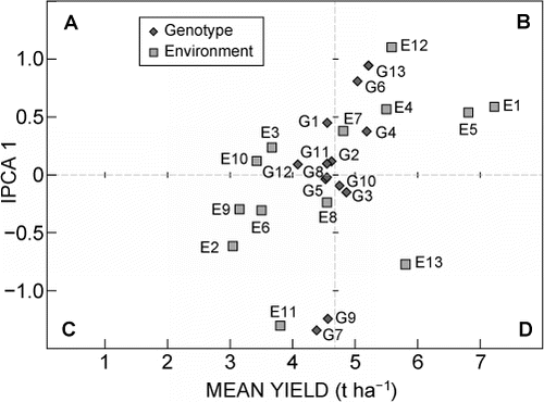
Genotypes in sections A and C had average grain yields that were lower than the grand mean. Any genotypes falling close to the point of origin of the multiplicative axis (IPCA 1) had lower interaction with most of the environments, and were stable. Genotypes located beyond 1 and -1 showed a high interactive behaviour with environments close to them and were generally unstable. Similarly, environments with IPCA 1 scores near zero had little interaction with genotypes, and also had low discrimination of genotypes, whereas those with IPCA scores beyond 1 (±) discriminated genotypes more effectively.

Most genotypes had IPCA 1 scores ±1. BR993 and Obatanpa had large negative IPCA scores of -1.34 and -1.24, respectively, whereas PAN 6479 had a large and positive IPCA 1 score of 0.94. COMP 4 and ZM621 had near zero IPCA 1 scores of 0.02 and 0.03, respectively (Figure 1). Other genotypes that had low IPCA 1 scores, in their decreasing order, included Nelson's Choice (0.090), Okavango (0.091) and Afric 1 (0.10).

Mkhwezo 3 and Gogozayo 3 had IPCA 1 scores of -1.30 and 1.20, respectively, and these were the furthest from zero (±). On the other hand, Mqekezweni 3 (0.11), Gogozayo 1 (0.23) and Jixini 2 had IPCA 1 scores that were close to zero. PAN 6479 and ZM627 showed high interactive behaviour with Gogozayo 3, whereas BR993 and Obatanpa interacted strongly with Mkhwezo 3.

Which variety won in which environment?

An AMMI 2 biplot was plotted using IPCA 1 and IPCA 2 scores for both genotypes and environments (Figure 2). The biplot showed that genotypes PAN 6479, Okavango, ZM627, BR993, Afric 1 and Obatanpa were the furthest from the origin, and expressed a highly interactive behaviour (positive or negative) with specific environments. Connecting the extreme genotypes with lines formed a polygon. Lines perpendicular to the sides of the polygon were also drawn and these formed seven sectors of which three had environments clearly assigned to a genotype at the summit of the polygon (Figure 2).

Figure 2: Additive main effects and multiplicative interaction 2 biplot for IPCA 1 vs IPCA 2 scores for environments and genotypes

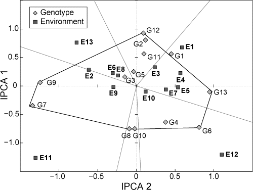
Going in a clockwise direction, Mqekezweni 1 (E1), Gogozayo 1 (E3), Jixini 1 (E4), Mqekezweni 2 (E5) and Gogozayo 2 (E7) fell into sector one and the summit genotype was PAN 6479 (G13), which was the highestyielding variety in this environment (Figure 2). ZM627 (G6) was the summit genotype in the second sector, containing Mqekezweni 3 (E10) and Gogozayo 3 (E12). The last sector contained environments Mkhwezo 3 (E11) and Qxididi 2 (E9) and these had BR993 (G7) and Obatanpa (G9) as their summit varieties (Figure 2).

Variety and environment stability as determined by AMMI stability values

Overall, there was a wide range in ASVs across the genotypes (Table 7). The majority of varieties had an ASV of less than 1. BR993 was the most unstable variety, having the highest index of 1.648. It was followed by Obatanpa with 1.493, ZM627 with 1.213 and PAN 6479 with 1.139. ZM621 and ZM501 had the lowest ASVs of 0.239 and 0.254, respectively (Table 7).

Table 7 AMMI stability values (ASV) for the genotypes

Genotype	ASV
ZM 305	0.779
ZM 423	0.815
ZM 501	0.239
ZM 525	0.780
ZM 621	0.254
ZM 627	1.213
BR993	1.648
COMP 4	0.752
Obatanpa	1.493
AFRIC 1	0.760
Nelson's Choice	0.574
Okavango	0.931
PAN 6479	1.139

There was wide variation in ASVs observed across the environments. Mkhwezo 3 and Gogozayo 3 had the highest ASV indices of 2.01 and 1.791, respectively, whereas Mqekezweni 3 had the lowest ASV index of 0.175 (Table 8).

Table 8: AMMI 2 genotype recommendations for each environment and yield improvements brought about by first recommendations. ASV = AMMI stability values

Environment	Score	1	2	3	4	ASV
Mqekezweni 1	0.5878	PAN 6479	ZM 423	ZM 305	ZM 627	0.977
Mkhwezo 1	-0.6149	Obatanpa	BR 993	ZM 501	ZM 423	0.791
Gogozayo 1	0.2381	PAN 6479	ZM 525	ZM 627	ZM 423	0.433
Jixini 1	0.567	PAN 6479	ZM 627	ZM 525	ZM 305	0.717
Mqekezweni 2	0.5378	PAN 6479	ZM 627	ZM 525	ZM 305	0.646
Mkhwezo 2	-0.3071	Obatanpa	ZM 501	ZM 525	PAN 6479	0.432
Gogozayo 2	0.3794	PAN 6479	ZM 627	ZM 525	ZM 501	0.460
Jixini 2	-0.2382	ZM 525	PAN 6479	ZM 501	Obatanpa	0.339
Qxididi 2	-0.2971	ZM 525	PAN 6479	Obatanpa	ZM 501	0.357
Mqekezweni 3	0.1198	PAN 6479	ZM 525	ZM 627	ZM 501	0.175
Mkhwezo 3	-1.3028	BR 993	Obatanpa	AFRIC 1	COMP 4	2.010
Gogozayo 3	1.1024	ZM 627	PAN 6479	ZM 525	AFRIC 1	1.791
Qxididi 3	-0.7722	Obatanpa	BR 993	ZM 423	ZM 501	1.198

AMMI variety recommendation for environments

The first-choice selection based on AMMI estimates, in six out of 13 environments, was PAN 6479 (Table 8). This was followed by Obatanpa, in three environments, and ZM525, in two environments. ZM525 and PAN 6479 had the most appearances (10 and nine out of 13 environments, respectively) in the top four variety recommendations, whereas COMP 4 had the least appearances (one out of 13).

Yield improvements were computed by comparing the AMMI adjusted grain yield means of each genotype recommended as the top performer by AMMI 2 within each environment and the environment mean, and obtaining the percentage increment. Recommending genotypes brought about differential yield improvements that ranged from -38% to 149.3% (results not shown). Recommending ZM525 to Qxididi 3 gave the highest yield improvement of 149.0%. On the other hand, recommending Obatanpa to Qxididi 2 gave a negative yield improvement of 38.85% (results not shown).

Discussion

Superior varieties of maize need to be adapted to specific and/or broad environments of the EC so as to ensure that yield stability and economic profit are realised by farmers. Yield performance of different maize genotypes is often affected by environmental conditions (Nakitandwe et al. 2005). The study of GEI can be used to identify varieties suitable for resource-poor farmers growing maize in diverse and stress-prone environmental conditions, based on their stability. Whilst in this study GEI was only significant at 10% in the AMMI, it was significant at 5% in the general ANOVA.

The observed GEI in the combined analysis could have been due to the contribution of the environment SS to the total variation in grain yield as observed by wide variation of yield obtained per environment and the dramatic change in rank position (crossover GE) by most genotypes within and across environments. Results observed are similar to those obtained by Mohammadi et al. (2007) and Akpalu et al. (2008). These authors highlighted that such changes in genotype ranking could be exacerbated by seasonal effects. However, the observed non-significant season main effect could be because increasing the number of seasons must have reduced the effect of season as a possible source of error during analysis, thus increasing statistical precision. These findings, therefore, emphasise the importance of multiseasonal studies when recommending genotypes with good yield stability to farmers producing maize in fluctuating weather patterns. However, non-crossover GEI was also evidenced in this study since some varieties ranked consistently throughout some environments across the three seasons.

The observed estimates of ASVs demonstrated that most environments were generally stable, which could suggest that these environments had more than one limiting factor affecting performance of different genotypes. These findings were in line with those obtained by Muungani et al. (2007) and Yan et al. (2007), who further reported that no meaningful information on genotype performance can be obtained in such environments. On the other hand, the observed large interaction scores for environments such as Mkhwezo 3 (E11) and Qxididi 3 (E13) could suggest the presence of fewer stress factors, allowing effective discrimination of genotypes (Yan et al. 2007).

Environment potential determines the threshold to which a variety can perform (Ceccarelli et al. 1994). The AMMI 1 biplot and environment grain yields suggested that Qxididi and Mkhwezo can be considered as low potential environments, whereas Jixini, Gogozayo and Mqekezweni could be of medium to high potential. When soil properties were considered, sites in low potential environments were characterised by low soil fertility due to inadequate major nutrients and carbon content, whereas high potential environments were generally fertile. These results agree with Ndufa (2001) who showed that maize yields are low if grown in soils depleted of nutrients and soil organic matter. In such environments, farmers should change current strategies for management of soil fertility to obtain the full benefits of stress-tolerant genotypes with high yield potentials (Nakitandwe et al. 2005).

High yields attained by PAN 6479 (G13) were possibly due to hybrid vigour. By nature, hybrids are genetically stable and possess hybrid vigour. These results agree with those obtained by Muungani et al. (2007), who observed superior performance of hybrids over OPVs. These results are also in agreement with findings by Pixley and Bänziger (2004), who reported that hybrid varieties outperform OPVs by at least 18% under suboptimum and optimum conditions. Furthermore, this hybrid variety was developed in South Africa, which could have given it adaptive advantages over the exotic OPVs. However, yield fluctuations by this variety were more pronounced across environments when compared to some CIMMYT OPVs, such as ZM 501 and ZM621, which did not show dramatic rank changes across the environments. Therefore, the recommendation of such stable OPVs for resource-poor farmers could result in better yield stability in diverse agroecologies than the use of hybrid varieties. On the other hand, the observed poor performance of BR993 and COMP 4, both tropical varieties, could be due to poor adaptation of these genotypes to the temperate environments that were tested in the EC.

The differences in yield performance and stability observed among the genotypes could also have been due to the differences in their genetic structure and morphological characteristics. Locally grown OPVs were moderately stable when compared with the new genotypes. However, they were not high yielding. This suggests that these varieties have been bred for environments in the EC, but have a low yielding potential. On the other hand, the observed stable performance of varieties such as ZM305, ZM501, ZM423 and ZM627 could be attributed to the intensive screening for tolerance to various stress conditions by CIMMYT, making them stable across different environments. The findings of this study agree with Muungani et al. (2007) who observed better stability with early-maturing CIMMYT OPVs across stress-prone environments.

Conclusions

Genotype × environment interaction was significant, resulting in varieties showing specific and wide adaptation to the environments. The best-performing genotype was PAN 6479, confirming superiority of hybrids over OPVs. This was followed by ZM525 and ZM627. The worst-performing genotypes were Okavango, BR993 and ZM 621. PAN 6479, BR 993, Obatanpa and ZM627 were unstable genotypes. ZM501 was the most stable variety, and showed no significant yield difference with PAN 6479. ZM621 was equally stable, though it was low yielding. PAN 6479 and ZM627 showed specific adaptations to high- and medium- potential environments. BR993 and Obatanpa were more suited to environments with low-yielding potential, such as Qxididi and Mkhwezo, since improvement of environmental conditions did not improve their yield.

Most environments were generally stable. Environments in the first two seasons were the most representative environments, whereas third season environments, with the exception of Mqekezweni, could be used to discriminate stable and unstable varieties. The ‘ideal’ environment for discriminating genotypes was Qxididi. This environment, and others similar to it, could be used in future GEI trials.

ZM525 could be recommended to high-potential environments that have low rainfall but good soil properties for water retention. ZM501, along with ZM627, ZM423 and ZM305, could be used across several environments in the EC. However, evaluations over more seasons are needed to substantiate these findings.

Acknowledgements

Funding from the Technology Innovation Agency (TIA) through grant PB111/08 is gratefully acknowledged.

References

- Admassu S, Nigussie M, Zelleke H. 2008. Genotype-environment interaction and stability analysis for grain yield of maize (Zea mays L.) in Ethiopia. Asian Journal of Plant Sciences 7: 163–169.
- Akpalu W, Hassan RM, Ringler C. 2008. Climate variability and maize yield in South Africa. IFPRI Research Brief 15-10. Washington, DC: IFPRI. Available at http://wwwifpriorg/publication/climate-variability-and-maize-yield-south-africa-0 [accessed 11 October 2010].
- Asfaw A, Alemayehu F, Gurum F, Atnaf M. 2009. AMMI and SREG GGE biplot analysis for matching varieties onto soybean production environments in Ethiopia. Scientific Research and Essay 4: 1322–1330.
- Bänziger M, Setimela PS, Hodson D, Vivek B. 2005. Breeding for improved abiotic stress tolerance in maize adapted to southern Africa. Agricultural Water Management 80: 212–224.
- Bembridge TJ. 2000. Guidelines for rehabilitation of small-scale farmer irrigation schemes in South Africa. WRC Report no. 891/1/00. Pretoria: Water Research Commission.
- Ceccarelli S, Erskine W, Hamblin J, Grando S. 1994. Genotype by environment interaction and international breeding programmes. Experimental Agriculture 30: 177–187.
- Fanadzo M, Chiduza C, Mnkeni PNS, van der Stoep I, Stevens J. 2010. Crop production management practices as a cause for low water productivity at Zanyokwe irrigation Scheme. Water SA 36: 27–36.
- Fraser GCG, Monde N, van Averbeke W. 2003. Food security in South Africa: a case study of rural livelihoods in the Eastern Cape Province. In: Nieuwoudt L, Groenewald J (eds), The challenge of change: agriculture, land and the South African economy. Pietermaritzburg: University of Natal Press. pp 171–183.
- Gabriel KR. 1978. Least squares approximation of matrices by additive and multiplicative models. Journal of the Royal Statistical Society, Series B (Methodological) 40: 186–196.
- Gadzirayi CT, Mutandwa E, Chihiya Y, Chitsa T. 2006. An assessment on the use of open pollinated varieties among small-holder farmers in Zimbabwe. Electronic Journal of Environmental and Agricultural and Food Chemistry 5(6): 1590–1597.
- Gomez KA, Gomez AA. 1984. Statistical procedures for agricultural research. New York: John Wiley and Sons.
- IUSS Working Group WRB. 2006. World reference base for soil resources 2006. World Soil Resources Reports 103. Rome: Food and Agriculture Organization of the United Nations. Available at ftp://ftp.fao.org/agl/agll/docs/wsrr103e.pdf [accessed 14 February 2014].
- Kang SM, Balzarini MG, Guerra JLL. 2004. Genotype-by-environment interaction. In: Saxton AM (ed.), Genetic analysis of complex traits using SAS®. Cary: SAS Institute. pp 69–94.
- Leeuvner DV. 2005. Genotype × environment interaction for sunflower hybrids in South Africa. MSc thesis, University of Pretoria, South Africa.
- Ma'ali SH. 2008. Additive mean effects and multiplicative interaction analysis of maize yield trials in South Africa. South African Journal of Plant and Soil 25: 185–193.
- Magorokosho C, Vivek BS, MacRobert J. 2008. Characterization of maize germplasm grown in eastern and southern Africa: results of the 2007 regional trials coordinated by CIMMYT. Harare: CIMMYT. Available at http://repository.cimmyt.org/xmlui/bitstream/handle/10883/1305/95633.pdf?sequence=1 [accessed 14 February 2014].
- MEDPT (Masifunde Education and Development Project Trust). 2010. Threats to the food security and food sovereignty in the Eastern Cape. Masifunde: MEDPT.
- Mkhari JJ, Matlebjane MR, Dlomu KP, Mudau ND, Mashingaidze K. 2006. Case study of a community-based seed production scheme in two districts of the Limpopo province, South Africa. In: Setimela PS, Kosina P (eds), Strategies for strengthening and scaling up community-based seed production. Mexico, DF: CIMMYT. pp 14–19. Available at http://repository.cimmyt.org/xmlui/bitstream/handle/10883/791/89218.pdf?sequence=1 [accessed 14 February 2014].
- Mohammadi R, Arrian M, Shabani A, Daryaei A. 2007. Identification of stability and adaptability in advanced durum genotypes using AMMI analysis. Asian Journal of Plant Sciences 6: 1261–1268.
- Muungani D, Setimela PS, Dimairo M. 2007. Analysis of multi-environment, mother-baby trial data using GGE biplots. African Crop Science Conference Proceedings 8: 103–112.
- Nakitandwe J, Adipala E, El-Bedewy R, Wagoire W, Lemaga B. 2005. Adaptability of sift potato genotypes in different agro-ecologies of Uganda. African Crop Science Journal 13: 107–116.
- Ndufa JK. 2001. Nitrogen and soil organic matter benefits to maize by fast-growing pure and mixed species legume fallows in western Kenya. PhD thesis, Imperial College at Wye, University of London, UK.
- Pixley K, Bänziger M. 2004. Open-pollinated maize varieties: a backward step or valuable option for farmers? In: Friesen DK, Palmer AFE (eds), Integrated approaches to higher maize productivity in the new millenium. Proceedings of the Seventh Eastern and Southern Africa Regional Maize Conference, 11–15 February 2002, Nairobi, Kenya. Nairobi: CIMMYT and KARI. pp 22–28.
- Purchase JL. 1997. Parametric analysis to describe genotype × environment interaction and yield stability in winter wheat. PhD thesis, University of Free State, South Africa.
- Setimela PS, Viveka B, Banziger M, Crossa J, Maideni F. 2007. Evaluation of early to medium maturing open pollinated maize varieties in SADC region using GGE biplot based on the SREG model. Field Crops Research 103: 161–169.
- Soil Classification Working Group. 1991. Soil Classification – a Taxonomic System for South Africa. Memoirs on the Agricultural Natural Resources of South Africa no. 15. Pretoria: Department of Agricultural Development.
- South Africa Rain Atlas. 2011. South Africa Rain Atlas. Available at http://134.76.173.220/rainfall/index.html [accessed 14 February 2014].
- Yan W, Kang MS, Ma B, Woods S, Cornelius PL. 2007. GGE biplot vs. AMMI analysis of genotype-by-environment data. Crop Science 47: 641–653.
- Zobel RW, Wright MJ, Gauch HG. 1988. Statistical analysis of a yield trial. Agronomy Journal 80: 388–393.