Evaluation of an over-used coastal aquifer (Orissa, India) using statistical approaches

Abstract

This study evaluates an over-exploited aquifer (Balasor, India) and also explores the possibilities of sustainable management using several statistical approaches. First, bootstrap analysis indicates that groundwater pumping has resulted in the reduction of mean cultivated area as the average irrigation capacity per bore well dropped from 3.74 ha to 1.5 ha within a period of 10 years of operation. However, modelling the groundwater levels using the seasonal autoregressive integrated moving average (SARIMA) procedure showed no evidence of large-scale groundwater withdrawals. The derived models can be used for water table forecasting and also for infilling the missing observations. The empirical relationship among pumping test results indicated that well depth and aquifer thickness significantly influence the discharge from the aquifer. This discharge may have encouraged the resource-rich farmers to exploit the lower aquifer. Based on a contour plot, the zone of groundwater exploitation was estimated to vary from 25 to 60 m below the surface. Therefore, a uniform aquifer exploitation policy needs to be implemented to curb the vertical competition in exploiting the aquifer and to develop sustainable management of the groundwater.

Citation Panda, D. K. & Kumar, A. (2011) Evaluation of an over-used coastal aquifer (Orissa, India) using statistical approaches. Hydrol. Sci. J. 56(3), 486–497.

Résumé

Cette étude évalue un aquifère surexploité (Balasor, Inde) et explore également les possibilités de gestion durable á l'aide de plusieurs approches statistiques. Premièrement, l'analyse bootstrap indique que le pompage des eaux souterraines a entraîné une réduction de la surface moyenne cultivée tandis que la capacité moyenne d'irrigation par forage a chuté de 3.74 à 1.5 ha sur une période de 10 années d'opération. Cependant, la modélisation des niveaux des eaux souterraines à l'aide de la procédure du modèle saisonnier autorégressif à moyenne mobile intégrée (SARIMA) n'a pas apporté la preuve de prélèvements d'eau souterraine à grande échelle. Les modèles dérivés peuvent être utilisés pour la prévision de la nappe phréatique et aussi pour la reconstitution des observations manquantes. La relation empirique entre les résultats des essais de pompage a indiqué que la profondeur du puits et l’épaisseur de l'aquifère influencent de faon significative le débit de l'aquifère. Ce débit peut avoir encouragé les agriculteurs riches en ressources à exploiter l'aquifère inférieur. Sur la base des lignes de niveaux, il a été estimé que la zone d'exploitation des eaux souterraines a varié de 25 à 60 m sous la surface. Par conséquent, une politique d'exploitation de l'aquifère uniformisée doit être mise en uvre pour freiner la concurrence verticale dans l'exploitation de l'aquifère et pour développer la gestion durable des eaux souterraines.

Key words:

• groundwater level
• over-exploited aquifer
• bootstrapping
• SARIMA
• aquifer parameters

Mots clefs:

• niveau des eaux souterraines
• aquifère surexploité
• bootstrap
• SARIMA
• paramètres d'aquifère

Introduction

Groundwater has become an indispensable natural resource for human survival in the context of changing climate and population growth, due to the important role it plays in global food production and in meeting the drinking water demands for a large proportion of the global population. However, groundwater resources are depleting in different parts of the world as anthropogenic groundwater withdrawals exceed the natural recharge (Döll & Fiedler, 2007). In Asia, intensive groundwater irrigation is a kind of silent revolution and the source of social conflicts (Llamas & Santos, 2005). The annual groundwater use of India, Nepal, Bangladesh, Pakistan and China is around 300 km³, which accounts for

nearly half of the world's annual groundwater use (Shah et al., 2003). Climatic stresses in the form of droughts and increased temperatures also affect the groundwater resources (Loaiciga, 2003; Panda et al., 2007). Groundwater depletion is associated with water quality degradation, saline water intrusion, and land–atmosphere energy feedback change. Conspicuous social problems can also arise due to the “vertical” competition among the stakeholders in exploiting the aquifer. For example, groundwater depletion due to use of deep wells by wealthy farmers causes the drying up of the shallow wells of poor farmers located in the area of influence of the deep wells (Llamas, 2004).

In India, groundwater has played a pivotal role in the success of the green revolution, ensuring food security for a population over one billion. Its use has jumped from around 10–20 km³ before 1950 to 240–260 km³ in 2000 (Shah et al., 2003). Around 60% of India's irrigated area is fed by groundwater (Sharma, 2009). In addition, groundwater meets 80% of the domestic water use in rural areas and 50% of the water use in the urban and industrial areas. Hard rock regions cover more than 60% of the geographical area. Natural recharge in these regions has been estimated to be only 4.1% to 19.7% of annual rainfall (Rangarajan & Athavale, 2000). Groundwater recharge only occurs if rainfall exceeds evapotranspiration. The recent increases in the frequency and magnitude of extreme rainfall events (Goswami et al., 2006) are likely to result in more runoff losses because of the slopping topography and hard rock soil. The GRACE (Gravity Recovery and Climate Experiment) satellite mission records reveal large-scale groundwater depletion in north and northwestern India because of the unsustainable consumption of groundwater for irrigation (Tiwari et al., 2009).

In Orissa, around 80% of the 36 million population depend on groundwater as a source for drinking water. In the densely populated coastal basin of Balasore, groundwater use for agriculture has resulted in declining groundwater levels and seawater intrusion (Rejani et al., 2003). It has been suggested that the annual gross per capita water availability in India will decline from 1820 m³ in 2001 to as low as 1140 m³ in 2050 (Gupta & Deshpande, 2004). Therefore, long-term policy measures need to be formulated for sustainable management of groundwater resources to meet future water requirements.

Recharge and discharge processes are complex, being primarily controlled by the climate, hydrogeological properties, surface water hydrological parameters, vegetation and land-use changes. Therefore, study of the response of an aquifer to anthropogenic and climatic stresses requires numerous parameters, which are less available and expensive to generate for large areas due to the high variability in hydrogeological properties. Lack of data is the primary reason for the smaller number of studies regarding impacts of anthropogenic and climatic stresses on groundwater in comparison to studies of surface water (Kundzewicz et al., 2007). However, groundwater level time series from monitoring networks are the principal source of information on the effect of hydrological and anthropogenic influences on groundwater systems (Alley et al., 2002; Environment Canada, 2004). A well-conceived monitoring network can provide early warning of degradation, and is thus capable of informing the policy makers for sustainable management of groundwater resources (Morris et al., 2003). But, the cost of maintenance and execution of groundwater monitoring networks is high. Several agencies use private wells, which are called the “well of opportunity”, to offset the cost of drilling. However, the scientific design of a groundwater monitoring network is the most important assignment to interpret the aquifer responses.

The primary objective of this study was to evaluate an overexploited aquifer (Balasor, India) and to develop a cost-effective monitoring network using non-parametric and parametric statistical procedures. Groundwater level monitoring data sets generated from the “National Hydrographic Network Stations” of the Central Ground Water Board (CGWB, 2000), and the pumping test data sets of the exploratory wells have been used in this study. The impact of the over-exploitation was studied using the non-parametric bootstrap technique. The temporal behaviour of the groundwater levels was examined using the seasonal autoregressive integrated moving average (SARIMA), which takes into account the seasonality of groundwater level of the observation wells (Tankersley & Graham, 1993). The modelling results can be used to assess the suitability of the existing monitoring network. Further, the empirical relationships among the aquifer characteristics were discussed. Using the surveyed data of the groundwater users, the zones of groundwater exploitation have been identified, which can be used for designing the monitoring network and also to aid policy formulation.

STUDY AREA

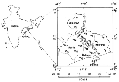
The study area, which is comprised of the Bhogorai, Jalesore, Baliapal and Basta blocks of the Balasore district of northeastern Orissa, is situated between latitudes 21°30′–22°0′N and longitudes 87°0′–87°30′E adjacent to the Bay of Bengal (Fig. 1). The area of the region is 1365 km². The study area has a subtropical humid climate with an average rainfall of 1712 mm and is endowed with a vast arable tract. Alluvium and sandy soils cover around 60% of the geographical area. Both the recent and older alluvium and crystalline granite gneiss form a good repository for groundwater. The water table occurs at various depths ranging from 10 to 300 m b.g.l. The underlying geological strata indicate that the study area has three confined aquifers that are separated by the clay layers of different thickness. The top aquifer, present at depths ranging from 2 to 60 m b.g.l., is the most exploited one. The groundwater exploitation for agriculture and allied activities has been estimated to be 26 600 ha, which is 71% higher than the safe yield of the aquifer. The saline water strata are found to exist over the fresh water zone in the second aquifer which ranges from 30 to 70 m b.g.l. within a 4 to 5 km wide tract along the coastline.

Fig. 1 Map of the study area (Balasore, Orissa). Locations of the 17 bore wells used for the pumping test are shown.

METHODS

Bootstrap estimation of confidence interval

The bootstrap is an intensive computational procedure, which uses resampling with replacement to reduce the uncertainties of the estimates (Efron & Tibishirani, 1993). The aim of the resampling is to mimic the random component of a process and to reduce the variance through averaging over numerous different partitions of the data. The main application of bootstrapping is to construct the confidence interval for the parameters of interest in situations where the distribution of the population and/or parameter is not known. In practice, the probability distribution of the population from which the sample comes is either not known or the sample size is too small to meet the distributional assumptions. The bootstrap is a non-parametric technique that helps in drawing valid statistical inferences when classical approaches cannot be employed. A bootstrap sample X* = (X*₁, X*₂, … , X* _n ) is obtained by randomly sampling n times with replacement from the original data points, X = (X ₁, X ₂, … , X_n ). Using a computer algorithm numerous independent bootstrap samples (S) (X*₁, X*₂, … , X*_S), each of size n, are generated. Corresponding to each of the S bootstrap samples (X* _S ), the parameters of interest , the bootstrap statistics, are calculated.

In this study, the percentile and standard methods have been used to find the confidence interval using 1000 bootstrap samples. For the percentile method, the lower and upper limits of the confidence interval can be represented as [ _lo, _up] = [ _S(α/2), _S(1-α)/2], where _S(α/2) is the (S(α/2))th value of the ordered . In the present study, the 95% confidence interval (α = 0.05) using 1000 bootstrap samples falls between 25th and 975th ordered . The standard method of finding the confidence interval assumes that the bootstrap estimates follow a normal distribution with the mean , and a standard error . The (1 – α) × 100% standard confidence interval is given by [ _lo, _up] = [ ± z _(α/2) ], where z follows a standardized normal variable.

Seasonal ARIMA modelling

In general, an ARIMA model is characterized by ARIMA (p,d,q) where, p, q, and d denote the order of autoregression, integration (differencing), and moving average, respectively. The corresponding seasonal multiplicative ARIMA model is represented by ARIMA (p,d,q) × (P,D,Q)_s with P, D and Q denoting the seasonal autoregression, integration (differencing), and moving average, respectively (see Box & Jenkins, 1976; Tankersley & Graham, 1993). The seasonal ARIMA is defined by:

1

where y_t is the original time series, e_t is a normal independently distributed white noise residual series with mean zero and variance σ². Here, Φ and Θ represent the ARIMA structure between the seasonal observations whereas φ and θ represent the within period non-seasonal ARIMA structure. Further, φ _p (B) and Φ _P (B^s ) are the non-seasonal and seasonal autoregressive operators of order p and P, respectively, and are given by:

2

3

Similarly, θ _q (B) and Θ _Q (B^s ) are the non-seasonal and seasonal moving average operators of order q and Q, respectively, and are given by:

4

5

Further, ^d and _s ^D are the non-seasonal and seasonal differencing operators of orders d and D, and are represented by:

6

7

The SARIMA procedure was used to model the groundwater levels time series of the monitoring wells. The time series model development involves three major steps. In the first identification step, the time series is analysed for stationarity and normality using appropriate differencing and transformations of the series. Further, the temporal correlation of the original and differenced series is identified by examining the autocorrelation (ACF) and partial autocorrelation (PACF) functions. In the second step, the autoregressive and moving average parameters of the identified model are estimated. To examine the adequacy and assumptions of the model, diagnostic checking is carried out in the third step. The analysis was carried out using the Statistical Package for the Social Sciences (SPSS, 2002).

RESULTS SAND DISCUSSION

Bootstrap confidence interval

More than 10 000 bore wells exist in the region to meet the irrigation requirements of the predominantly rice-based cropping system. Two of the three rice crops that are grown per year depend completely on groundwater. Due to over-exploitation of the groundwater, the water yielding capacity of the bore wells reduces after a few years of operation. This leads to the abandonment of existing wells and the search for new ones having a better aquifer in terms of the discharge capacity. Each year hundreds of bore wells are abandoned. Table 1 lists a few cases of wells abandoned due to groundwater level decline and the decline in irrigated area of the study region. The bootstrap samples indicated that the mean area irrigated at the beginning of operation of a bore well dropped from 3.74 ha to 1.50 ha. The lower and upper limit of the 95% confidence interval derived from the 1000 bootstrap samples also indicated substantial decline in groundwater levels and in the irrigated area (Table 2).

Table 1  Cases of groundwater level decline and associated decrease in irrigated area (source: Central Ground Water Board, 2000)

	Year of construction	Water table decline by 1996 (m)	Initial area irrigated (ha)	Area irrigated in 1996 (ha)
Case 1	1981	2.0	10.0	3.2
Case 2	1992	2.0	4.0	2.4
Case 3	1988	2.0	3.2	1.6
Case 4	1990	2.0	1.6	0.4
Case 5	1990	2.5	4.0	2.0
Case 6	1989	3.0	4.0	1.6
Case 7	1987	2.0	2.0	0.4
Case 8	1985	2.0	2.8	1.2
Case 9	1993	4.0	1.6	0.6

Table 2  Ninety-five percent onfidence intervals using the percentile and standard methods of bootstrap sampling

	Percentile method		Standard method
	Lower	Upper	Lower	Upper
Water level decline by 1996 (m)	2.00	2.89	1.96	2.82
Initial area irrigated (ha)	2.40	5.46	2.11	5.36
Area irrigated in 1996 (ha)	0.91	2.11	0.91	2.09

In order to understand the socio-economic dynamic of the groundwater stakeholders, a survey was conducted of 100 groundwater users selected through simple random sampling. Survey responses indicated that there is a “vertical” competition among the farmers in search of better aquifers as the rate of failure of the bore wells increases. The rich farmers owned the deeper bore wells and also those at greater distances from the residential area; they were able to bear the electrification cost at the distant locations. Further, the presence of the deep bore wells of the rich farmers was reducing the water yielding capacity of the nearer shallow wells owned by poor farmers. This was forcing the poor farmers either to purchase groundwater, i.e. groundwater marketing, or to lease out their land to the rich farmers. Therefore, policy measures need to be formulated for uniform digging and exploitation of aquifer.

Modelling groundwater levels

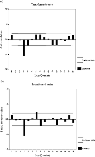
Groundwater levels were recorded on four occasions in a year (quarterly), i.e. during the pre-monsoon (April), monsoon (August), post-monsoon (November), and irrigation (January) periods. As the unit of the groundwater level record is metres below ground level (m b.g.l.), a greater value suggests that the water table occurs at greater depth from the surface. Inspection of the quarterly time series plots for each of the five monitoring wells in the study area indicated that all varied seasonally. For illustration, the time series plot of the groundwater level of one monitoring well (Jaleswar 73O-1A1) is presented (Fig. 2). Although groundwater levels showed high variability in recent years, no perceptible trend was observed inspite of the over-exploitation of the aquifer. Further, inspection of the autocorrelation (ACF) plots of the original time series of all the wells confirmed the presence of seasonal behaviour. For example, Fig. 3(a) shows the seasonal persistence with a 4-quarter cycle, i.e. peaks above the 95% confidence interval at lags equal to 4 and its multiples. The partial autocorrelation (PACF) plots also showed no cut off after one spike, indicating a strong seasonality (Fig. 3(b)). To remove the observed seasonal persistence of the original time series, all the time series were transformed by differencing once across lag = 4 quarters. Figure 4(a) indicates that the differenced series exhibits non-significant autocorrelations. The PACF plots of the differenced series also showed similar behaviour (Fig. 4(b)). Further, natural log (LN) transformation was performed to ensure normality of the differenced time series of all the wells.

Fig. 2 Time series plot of the quarterly water table (m b.g.l.) indicating the seasonal variability for a monitoring well (Jaleswar 73O-1A1).

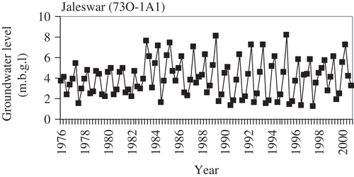
Fig. 3 (a) Autocorrelation (ACF) and (b) partial autocorrelation (PACF) plots for a monitoring well (Jaleswar 73O-1A1) showing clear seasonal variability in the time series. Solid lines represent the 95% confidence limit of white noise.

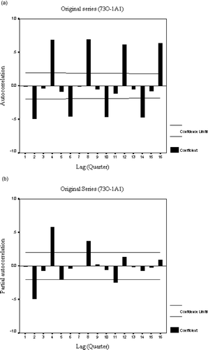
Fig. 4 (a) Autocorrelation (ACF) and (b) partial autocorrelation (PACF) plots of the differenced time series for a monitoring well (Jaleswar 73O-1A1). Transformation has resulted in stationarity in the time series.

The pattern of the ACF and PACF plots suggested the SARIMA behaviour of the groundwater level time series. In general, three forms of SARIMA models were found to explain the groundwater level fluctuations satisfactorily. Sensitivity of the SARIMA models was examined based on the model stability, residual whiteness, residual normality, residual homoscedasticity and goodness of fit. Two monitoring wells could be modelled by SARIMA(0,0,1)(0,1,1)₄, two by SARIMA(0,0,0)(0,1,1)₄, and one by SARIMA(0,0,1)(1,1,1)₄ (Table 3). The non-seasonal and seasonal moving average parameters, i.e. θ and Θ, with very low standard errors were found to be significant at the 5% level, i.e. the null hypothesis of the two-sided Student's t-test was rejected at the 5% significance level. Further, the seasonal autoregressive parameter Φ for the model SARIMA(0,0,1)(1,1,1)₄ was found significant at the 5% level. The non-significant parameters were removed from the models.

Table 3  Selected SARIMA models for the groundwater level time series

Monitoring station (well Id.)	Time series	ARIMA (p,d,q) (P,D,Q)4	SE	AIC	ESS (1998–2000)
Jaleswar (73O-1A1)	1976–2000	(0,0,1) (1,1,1)4	0.27	24.99	31.64
Bhogorai (73O-2B3)	1988–2000	(0,0,1) (0,1,1)4	0.23	0.92	2.53
Baliapal (73O-2B1)	1976–2000	(0,0,0) (0,1,1)4	0.39	88.68	11.07
Basta 1 (73O-2A1)	1970–2000	(0,0,1) (0,1,1)4	0.52	72.47	5.25
Basta 2 (73O-2A2)	1986–2000	(0,0,0) (0,1,1)4	0.39	45.43	8.33
SE: standard error: AIC: Akaike's information criterion; ESS: error sum of square.

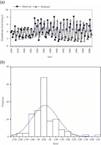
The selected models also have the minimum standard error (SE). Additionally, the Akaike's information criterion (AIC), which determines whether a model with more parameters is preferable to a model with fewer parameters, was used to select the models based on its minimum value. To further examine forecasting performances, the selected SARIMA models were fitted up to the year 1998, and the groundwater levels were forecast for the period 1999–2000 to enable comparison with the observed values. The error sum of square (ESS) of the predicted groundwater levels was less for all the models, except that of the Jaleswar (73O-1A1) station due to the presence of two outlying observations. However, the overall suitability of the model was not impaired as evident from the goodness of fit between the observed and predicted groundwater levels for the Jaleswar (73O-1A1) station (Fig. 5(a)). The normality assumption of the residuals of the selected models was examined using both the graphical and mathematical tests. For all the models, the histogram plots of the residuals were found to be approximately normally distributed (Fig. 5(b)). The Kolomogorov-Smirnov test of normality also indicated that the errors were normally distributed.

Fig. 5 (a) The predicted groundwater levels for the monitoring well (Jaleswar 73O-1A1) show a good fit with the observed values. (b) Comparison of the empirical histogram with normal distribution.

The results suggest that the SARIMA models do not differ much from each other in the number and type of parameters. Further, the magnitude of the parameters of the same SARIMA model did not differ greatly. This suggests that the aquifer system behaves in a consistent manner in the study area. The quarterly groundwater levels of the monitoring network show a cyclic behaviour with an annual elevated water table in August and a lower water table in April. This cycle is primarily driven by the monsoon rainfall during the summer months of June to September, which contributes more than 80% of the annual rainfall. The seasonal autoregressive terms of the water table, as evident from the ACF and PACF plots, are due to this recurring monsoon rainfall pattern. Further, the seasonal and non-seasonal moving average terms in all the SARIMA models, i.e. θ and Θ, suggest that the aquifer system recovers substantially within an annual time period from any one random recharge event. The small variation in the model parameters, and their magnitude, of the monitoring wells reflect the variations in the aquifer properties, groundwater withdrawal, and local climate. The SARIMA models developed in this study provide an improved approximation of the temporal behaviour of the groundwater levels. Forecasting water table levels using these models could be helpful for cost minimization of the existing monitoring network. For more effective groundwater planning and management, new monitoring wells need to be designed taking into account the aquifer characteristics, which govern the physical processes of the groundwater system of this over-exploited aquifer.

Pumping test results

Pumping test data of 17 exploratory bore wells were analysed to understand the hydraulic properties of the aquifer. Figure 1 shows that the location of the bore wells across the study area. Table 4 presents the pumping test results for the aquifer, including discharge, i.e. yield (Q), depth of well (D), thickness of aquifer (Th), transmissivity (T), and storativity (S). Although the depth of well (D) is not an aquifer characteristic, we have analysed this because of the present competition among groundwater stakeholders in exploiting the deeper aquifer in order to increase the water yielding capacity of wells. The discharge, which is an indirect aquifer characteristic that groundwater users measure during the installation of a bore well, shows high spatial variability ranging from 4.28 to 53.50 L s^-1, with an average of 21.13 L s^-1 for a the drawdown ranging from 5.83 to 15.60 m (Fig. 1, Table 1). The static groundwater level ranges from 2.13 to 10.68 m b.g.l. In general, the northern part of the study area showed a higher yielding capacity of the aquifer in comparison to the southern parts. The recharge and flow of groundwater is from north to south into the Bay of Bengal for the top aquifer. Further, the aquifer around the Subarnarekha River exhibited high discharge, suggesting a contribution from river seepage. In addition to the monsoon rainfall, the Subarnarekha River, with a flow of 4000 m³ s^-1 during the monsoon season, is one of the major sources of recharge of the basin (Rejani et al., 2003). In general, the rainfall and flow of the Subarnarekha River during the monsoon season determine the area to be covered by the non-monsoon (October to June) crops, i.e. those primarily irrigated by groundwater. The transmissivity also showed high spatial variability, ranging from 122.08 to 3415 m² d^-1 with an average of 1268.94 m² d^-1. In general, the observed high transmissivity of the study area implies that it will take less time to replace the water withdrawn during pumping.423 Col No: 236

Table 4  Pumping test results for 17 bore wells in the study area

Well	Depth (m)	Discharge (L s^-1)	Thickness (m)	Transmissivity (m^2 d^-1)	Storativity (× 10^-3)
w1	60.90	11.50	22.00	152.70	6.30
w2	48.70	11.28	17.06	1072.33	2.20
w3	88.40	31.00	30.48	933.40	3.06
w4	50.00	7.75	20.50	758.05	9.30
w5	94.50	27.50	33.80	1178.83	4.50
w6	42.00	12.17	17.00	2715.00	5.40
w7	40.00	17.91	19.00	3415.00	3.20
w8	91.50	20.90	31.08	336.76	3.80
w9	88.30	24.50	27.43	1979.40	2.70
w10	64.00	22.43	24.38	567.05	1.10
w11	64.30	34.16	21.34	1062.15	9.20
w12	82.30	28.98	21.53	689.50	6.50
w13	92.50	53.50	56.00	2695.21	1.20
w14	67.00	25.00	20.60	131.50	1.30
w15	35.00	14.81	18.50	1918.00	1.60
w16	79.24	11.50	18.46	122.08	7.10
w17	30.00	4.28	13.50	1845.00	15.80

Figure 6 displays the patterns and empirical linear relationships among the pumping test variables. Correlation coefficients among the depth, discharge, and thickness of the aquifer were significant at the 5% level, suggesting the considerable influence of each other. Visual patterns also indicate that the discharge of a well increases as the depth and thickness of the aquifer increases. Further, the thickness of the aquifer increases with respect to the depth of the aquifer. The functional forms of the relationships indicate that the depth and thickness of the aquifer are the significant explanatory variables of the models (Table 5). The transmissivity, which scattered around the specified range without any definite pattern (Fig. 6), showed the least empirical relationship with the other variables, even after logarithmic transformation. The weak relationship indicates that the transmissivity decreases with depth and increases with the thickness of the aquifer. Further, discharge increases with the transmissivity although it is not a significant explanatory variable (Table 5). The storativity values, which describe the change in volume of water for a unit change in water level per unit area, showed high variation ranging from 1.1 × 10^-3 to 15.8 × 10^-3 with an average of 4.95 × 10^-3. The patterns show that the storativity is weakly and inversely correlated with the other pumping test variables. Functional form also indicates that the storativity influences the discharge of the aquifer (significant at the 10% level).

Fig. 6 Patterns among the pumping test variables depth (m), discharge (L s^-1), thickness (m), transmissivity (m² d^-1), and storativity (10^-3) are displayed graphically. Correlation coefficients and visual patterns indicate that the depth, discharge, and thickness of the aquifer significantly influence each other. The transmissivity and storativity show greater spread of the data points with weak patterns.

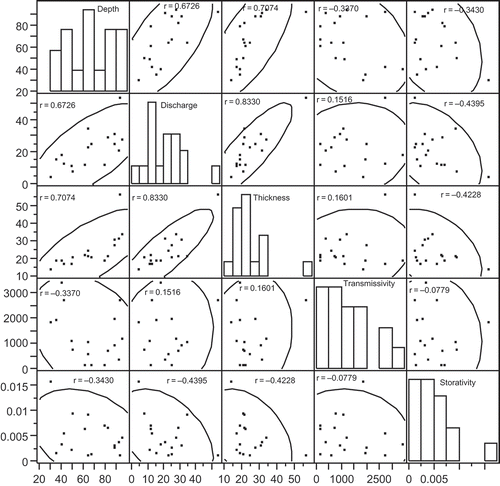
Table 5  Functional forms of the empirical relationships of the pumping test variables

Equation	F-ratio
Q = –3.17 + 0.37D*	12.39*
Q = –3.56 + 1.02Th*	34.00*
Th = 3.34 + 0.32D*	15.02*
Q = 18.81 + 0.0018T	0.35
Q = 27.93 – 1.37S	3.59
Q: discharge; D: depth of well; Th: thickness of aquifer; T: transmissivity; and S: storativity.
* indicates that the model and parameters are significant at the 5% level.

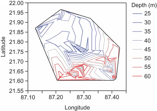
In general, the pumping test results indicate that a high proportion of the study area is suitable for groundwater extraction. However, it is important to safeguard the aquifer as vertical competition to dig deeper in order to get maximum yields make the aquifer unsustainable. Most of the groundwater stakeholders own private bore wells and therefore no records are available regarding the depth of their bore wells. In this study, 100 farmers were surveyed to aid understanding of the aquifer that they are exploiting. Analysis indicated that the mean well depth was 46.2 m with a standard deviation of 13.5 m. Contour plots of the bore well depths show clear spatial patterns of the aquifer exploitation zones (Fig. 7). Well depth varies from 25 to 60 m b.g.l. It is interesting to note that the northern and the central portion of the study area pump water from shallow depths. However, the southern and eastern parts use deeper bore wells. Groundwater is available at a depth of 25 to 30 m in the central parts where the river recharges the aquifer. These results are consistent with the spatial distribution of the aquifer parameter determined from the pumping tests. The presence of deep bore wells reduces the water yielding capacity of the nearer, shallow wells because of the high transmissivity of the aquifer. Therefore, a uniform well digging policy, based on the contour plots, needs to be ensured to enhance the aquifer sustainability. Further, new piezometers should be installed to capture the groundwater level dynamics of the zone of exploitation.

Fig. 7 Contour plot showing the spatial variability of bore well depths obtained from the surveyed data; the range is 25–60 m b.g.l.

CONCLUSIONS

This study shows that over-exploitation of an aquifer has led to decline of groundwater levels with a consequent decrease in irrigated area. The socio-economic links with groundwater irrigation shows that the richer farmers or landlords owned the deeper bore wells. This was forcing the poor farmers either to purchase water, or to lease out their land to rich farmers. Although groundwater levels of the existing monitoring wells showed high variability in recent years, no perceptible trend was observed in spite of over-exploitation of the aquifer. The SARIMA models developed in this study provide an improved approximation of the temporal behaviour of the groundwater levels. Forecasting water table levels using these models could be helpful for cost minimization of the existing monitoring network. The empirical relationships among pumping test results indicated that well depth and aquifer thickness significantly influence the discharge of the aquifer. The depth of exploited aquifer should be considered when designing the monitoring network. A uniform bore hole depth policy needs to be implemented to safeguard the aquifer.

Acknowledgements

We appreciate the reviewers for their constructive comments and suggestions, which significantly improved the quality of the manuscript.

REFERENCES

- Alley , W. M. , Healy , R. W. , LaBaugh , J. W. and Reilly , T. E. 2002 . Flow and storage in groundwater system . Science , 296 : 1985 – 1990 .
- Box , G. E. P. and Jenkins , G. M. 1976 . Time Series Analysis: Forecasting and Control , Englewood Cliffs, NJ : Prentice Hall .
- Central Ground Water Board . 2000 . Groundwater Resources and Development Potentials of Balasore District, Orissa , Bhubaneswar, India: CGWB .
- Döll , P. and Fiedler , K. 2007 . Global-scale modeling of groundwater recharge . Hydrol. Earth System Sci. Discuss. , 4 : 4069 – 4124 .
- Efron , B. and Tibishirani , R. J. 1993 . An Introduction to the Bootstrap , New York : Chapman & Hall .
- Canada , Environment . 2004 . Threats to Water Availability in Canada. Burlington, ON: National Water Research Institute, NWRI Scientific Assessment Report Series no. 3 and ACSD Scientific Assessment Series no. , 1 : 77 – 84 .
- Goswami , B. N. , Venugopal , V. , Sengupta , D. , Madhusoodanan , M. S. and Xavier , P. K. 2006 . Increasing trend of extreme rain events over India in a warming environment . Science , 314 : 1442 – 1445 .
- Gupta , S. K. and Deshpande , R. D. 2004 . Water for India in 2050: first-order assessment of available option . Current Science , 86 ( 9 ) : 1216 – 1224 .
- Kundzewicz , Z. W. , Mata , L. J. , Arnell , N. W. , Döll , P. , Kabat , P. , Jiménez , B. , Miller , K. A. , Oki , T. , Sen , Z and Shiklomanov , I. A. 2007 . “ Freshwater Resources and Their Management. Climate Change 2007: Impacts, Adaptation and Vulnerability ” . In Contribution of Working Group II to the Fourth Assessment Report of the Intergovernmental Panel on Climate Change , Edited by: Parry , M. L. , Canziani , O. F. , Palutikof , J. P. , Hanson , C. E. and van der Linden , P. J. Cambridge : Cambridge University Press .
- Llamas , R. 2004 . Water and Ethics: Use of Groundwater , Paris : UNESCO .
- Llamas , M. R. and Santos , P. M. 2005 . Intensive groundwater use: silent revolution and potential source of social conflicts . J. Water Resour. Plan. Manage. , 131 ( 5 ) : 337 – 341 .
- Loaiciga , H.A. 2003 . Climate change and groundwater . Ann. Assoc. Am. Geogr. , 93 : 30 – 41 .
- Morris , B. L. , Lawrence , A. R. L. , Chilton , P. J. C. , Adams , B. , Calow , R. C. and Klinck , B. A. 2003 . Groundwater and Its Susceptibility to Degradation: A Global Assessment of the Problem and Options for Management , Nairobi, Kenya : United Nations Environment Programme, Early Warning and Assessment Report Series, RS 03-3 .
- Panda , D. K. , Mishra , A. , Jena , S. K. , James , B. K. and Kumar , A. 2007 . The influence of drought and anthropogenic effects on groundwater levels in Orissa, India . J. Hydrol. , 343 : 140 – 153 .
- Rangarajan , R. and Athavale , R. N. 2000 . Annual replenishable ground water potential of India-an estimate based on injected tritium studies . J. Hydrol. , 234 : 38 – 53 .
- Rejani , R. , Jha , M. K. , Panda , S. N. and Mull , R. 2003 . Hydrologic and hydrogeologic analysis in a coastal groundwater basin, Orissa, India . Appl. Engng Agric. , 19 : 177 – 184 .
- Shah , T. , Roy , A. D. , Qureshi , A. S. and Wang , J. 2003 . Sustaining Asia's groundwater boom: an overview of issues and evidence . Natural Resour. Forum , 27 : 130 – 140 .
- Sharma , K. D. 2009 . Groundwater management for food security . Current Science , 96 ( 11 ) : 1444 – 1447 .
- SS , SP . 2002 . SPSS 11.5 Brief Guide, version 11.5 , Chicago : SPSS Inc .
- Tankersley , C. D. and Graham , W. D. 1993 . Comparison of univariate and transfer function models of groundwater fluctuations . Water Resour. Res. , 29 ( 10 ) : 3517 – 3533 .
- Tiwari , V. M. , Wahr , J. and Swenson , S. 2009 . Dwindling groundwater resources in northern India from satellite gravity observations . Geophys. Res. Lett. , 36 : L18401 doi: doi:10.1029/2009 GL 039401