Trimmed L-moments (1,0) for the generalized Pareto distribution

Abstract

Statistical analysis of extremes is often used for predicting the higher return-period events. In this paper, the trimmed L-moments with one smallest value trimmed—TL-moments (1,0)—are introduced as an alternative way to estimate floods for high return periods. The TL-moments (1,0) have an ability to reduce the undesirable influence that a small value in the statistical sample might have on a large return period. The main objective of this study is to derive the TL-moments (1,0) for the generalized Pareto (GPA) distribution. The performance of the TL-moments (1,0) was compared with L-moments through Monte Carlo simulation based on the streamflow data of northern Peninsular Malaysia. The result shows that, for some cases, the use of TL-moments (1,0) is a better option as compared to L-moments in modelling those series.

Citation Ahmad, U.N., Shabri, A. & Zakaria, Z.A. (2011) Trimmed L-moments (1,0) for the generalized Pareto distribution. Hydrol.Sci. J. 56(6), 1053–1060.

Résumé

L'analyse statistique des extrêmes est souvent utilisée pour prévoir les événements de longues périodes de retour. Dans cet article, on propose l'utlisation des L-moments tronqués où la plus petite valeur a été ôtée—TL-moments (1,0)—comme alternative pour l'estimation des crues de longues périodes de retour. Les TL-moments (1,0) permettent de réduire l'influence négative qu'une valeur faible dans l'échantillon statistique pourrait avoir sur une période de retour importante. L'objectif principal de cette étude est d'exprimer les TL-moments (1,0) de la distribution de Pareto généralisée (GPA). Les résultats obtenus avec les TL-moments (1,0) ont été comparés avec ceux des L-moments par simulation de Monte Carlo en utilisant des données de débits du nord de la péninsule Malaise. Ces résultats montrent que, dans certains cas, il est préférable d'utiliser les TL-moments (1,0) plutôt que les L-moments pour la modélisation de ces séries.

Key words:

• L-moments
• TL-moments
• generalized Pareto distribution
• parameter estimation

Mots clefs:

• L-moments
• TL-moments
• généralisée de Pareto
• estimation des paramètres

INTRODUCTION

Flood is a natural disaster that occurs world-wide. Since floods may damage property, crops and people's homes, as well as cause loss of life, preventing floods is very important. A crucial problem in hydrological design is, thus, the estimation of high-flow quantiles. This estimation is very useful in the design of bridges, dams, detention ponds, etc., and by having an accurate estimation of flood frequency, the safety of the structure can be increased. Flood frequency analysis (FFA) is the most suitable method for such a case (Stedinger et al. 1992).

The main problem in FFA is the estimation of the parameters. There are a few methods that can be used for parameter estimation, such as method of moments (MOM), the maximum likelihood method (MLM), and the least squares method (LS). Hosking (1990) introduced the L-moments method as an alternative to product moments to facilitate the estimation process in frequency analysis. L-moments possess several advantages over any other product moments; for example, the L-moment ratio estimates on scale, location and shape are nearly unbiased for any probability distribution which might be observed. According to Vogel and Fennessey (1993), product moments and moments ratio methods have been criticized for being oversensitive towards the upper part of the distribution and the outliers. Wang (1990) questioned whether the L-moments method is too sensitive towards the lower part of the distributions giving an insufficient weight to large sample value.

Therefore, in this paper, the method of trimmed L-moments, with one smallest value trimmed—TL-moments (1,0)—is proposed to characterize the upper part of the distributions and extreme flood events. Estimation of the generalized Pareto (GPA) distribution by using TL-moments (1,0) is formulated. Then, the comparison of the performance of L-moments and TL-moments (1,0) is done using both real and simulated data. TL-moments (1,0) and L-moments ratio diagrams are constructed using annual maximum streamflow data for stations across northern Peninsular Malaysia, namely, Kedah, Perak, Perlis and Penang, to examine the ability of GPA distribution to model those series.

TL-MOMENTS (1,0)

Trimmed L-moments (TL-moments) were introduced by Elamir and Seheult (2003) with a view to increasing awareness towards the outliers. The TL-moments give zero weight to the extreme value, are easy to compute and are said to be more robust than the L-moments in the presence of outliers. A few studies have been done with the TL-moments method, for example, Asquith (2007), Hosking (2007), Abdul Moniem (2007, 2010), and Abdul Moniem and Selim (2009). However, in these studies, the researchers focused only on symmetrical cases where they trimmed one smallest and one largest values (t ₁ = t ₂ = 1) from the conceptual sample. Elamir and Seheult (2003) defined the rth TL-moments, as follows:

(1)

From equation (1)(1), clearly TL-moments reduce to L-moments when t ₁ = t ₂ = 0. Based on a few studies (Cunnane 1987, Wang 1990, Bhattarai 2004), we propose TL-moments (1,0), where one smallest value is trimmed (t ₁ = 1, t ₂ = 0) from the conceptual sample. Let Y ₁, …, Y_r be a conceptual sample of size r from a continuous distribution with quantile function x(F). For each r, we increase the conceptual sample size from r to r+1 and work only the expectations of r-order statistics by trimming one smallest value. We denote such modification as rth TL-moments (1,0), , and define as follows:

(2)

The expectations of Y_ir can be written as:

(3)

Based on equation (2)(2), the first four of TL-moments (1,0) can be written as:

(4)

(5)

(6)

(7)

In particular, provides a measure of the location of the distribution, is the measure of the scale, is a measure of the skewness and is a measure of kurtosis respectively. The population TL-skewness and TL-kurtosis can be defined as:

(8)

(9)

Unbiased estimates of TL-moments (1,0) can be based on the sample TL-moments (1,0) from an ordered data sample . Based on the equation of sample TL-moments proposed by Elamir and Seheult (2003), an unbiased estimate of the rth TL-moment (1,0), is:

(10)

The sample TL-skewness and TL-kurtosis can be defined as:

(11)

(12)

TL-MOMENTS (1,0) OF GENERALIZED PARETO DISTRIBUTION

The generalized Pareto (GPA) distribution is one of the distributions which often provides the best approximation to flood flow data and has been the subject of many studies. Abdul Moniem and Selim (2009) studied the TL-moments and L-moments estimation for GPA distribution. Saf (2008) employed the GPA distribution in regional flood frequencies analysis using L-moments for the Buyuk and Kucuk Menderes river basins of Turkey. The probability density function of the GPA distribution is:

(13)

where ξ, α and k are location, scale and shape parameters, respectively. The corresponding cumulative distribution function is:

(14)

The value of x can be in the range of for k < 0 and for k > 0. The quantile function for GPA distribution can be written as:

(15)

Substituting equation (15)(15) into equations (4)(4) (5) (6)–(7)(7) and computing the expectations yields:

(16)

(17)

(18)

(19)

The three parameters α, ξ and k in the GPA distribution can then be estimated by matching the first three TL-moments (1,0) to their sample estimates:

(20)

(21)

(22)

EXAMPLES

The effects of using TL-moments (1,0) were shown in this study by using the data of streamgauge Slim on the Slim River, Perak, Malaysia. The data set, which contains 33 annual maximum flows covering the years 1977–2009, has been provided for this study by Department of Irrigation and Drainage, Ministry of Natural Resources and Environment, Malaysia. The station has a catchment area of 455 km².

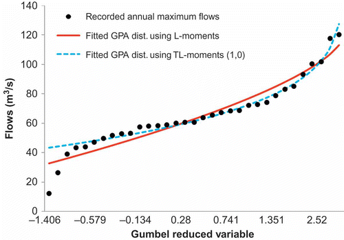
Figure 1 shows two GPA distribution curves fitted to the first data series, one by using L-moments and the other by using TL-moments (1,0). Clear conclusions cannot be drawn from just one example. However, Fig. 1 seems to suggest that distribution curves fitted by using L-moments are influenced too much by small annual maximum flows, leading to poorer prediction compared to TL-moments (1,0). In contrast, the curves fitted by matching TL-moments (1,0) better capture the trends shown especially by the larger flows. The TL-moments (1,0) seem to be less influenced by small annual maximum flows. So, using TL-moments (1,0) is expected to be more reasonable than L-moments estimates.

Fig. 1 Fitting the GPA distribution to annual maximum flows at the streamgauge Slim at Slim River, Perak, Malaysia.

MONTE CARLO SIMULATIONS

To investigate the effects of using TL-moments (1,0) on high quantile estimation, a Monte Carlo simulation study was applied. In each simulation, the generated samples from N = 10 000 replicates are used to obtain the bias and root mean square error (RMSE) values of quantile estimator. Three different sample sizes were applied in this study: n = 15, 25 and 50. The bias and RMSE were computed using equations (23)(23) and (24) as follows:

(23)

(24)

where are estimated values whereas θ is the true value of the quantile and N is the number of generated samples of size n.

Known parent distribution

For known underlying distribution, it is important to see how the estimation is affected by using various methods when the assumed distribution function follows the parent distribution function. This is studied here by fitting the GPA distribution function to the generated GPA samples. The values of the parameters of scale and location are set to 0 and 1, respectively with different values of k = −0.4, −0.3, −0.2, −0.1, 0.1, 0.2, 0.3, 0.4.

The Bias values were obtained for quantile function x(F) for F = 0.98, F = 0.987 and F = 0.99 for all sample sizes, n, as shown in Table 1. Table 1 shows that the quantile estimates are almost unbiased for positive k, regardless of whether L-moments or TL-moments (1,0) are used. When k becomes more negative, the quantile estimator becomes more positively biased. The bias values obtained using TL-moments (1,0) are smaller than using L-moments for positive k values. However, as k becomes negative, TL-moments (1,0) result in greater bias than if using L-moments.

Table 1  Bias of x(F) estimator fitting the GPA distribution to generated GPA samples for all sample sizes

k	Method	n = 15			n = 25			n = 50
		F = 0.98	F = 0.987	F = 0.99	F = 0.98	F = 0.987	F = 0.99	F = 0.98	F = 0.987	F = 0.99
−0.4	L-moments	1.041	1.254	1.374	0.700	0.846	0.925	0.472	0.574	0.632
	TL-moments (1,0)	1.185	1.496	1.701	0.801	1.022	1.168	0.536	0.686	0.785
−0.3	L-moments	0.537	0.567	0.543	0.355	0.370	0.348	0.152	0.139	0.107
	TL-moments (1,0)	0.660	0.755	0.784	0.432	0.490	0.502	0.200	0.214	0.204
−0.2	L-moments	0.291	0.253	0.187	0.133	0.095	0.041	0.070	0.047	0.014
	TL-moments (1,0)	0.387	0.391	0.356	0.191	0.177	0.141	0.100	0.090	0.068
−0.1	L-moments	0.116	0.053	−0.022	0.049	0.004	0.016	0.034	0.012	−0.013
	TL-moments (1,0)	0.188	0.148	0.089	0.087	0.057	−0.046	0.053	0.038	0.017
0.1	L-moments	0.006	−0.045	−0.094	−0.004	−0.035	−0.064	−0.002	−0.016	−0.031
	TL-moments (1,0)	0.042	−0.001	−0.047	0.013	−0.015	−0.042	0.007	−0.006	−0.018
0.2	L-moments	−0.012	−0.053	−0.091	−0.015	−0.038	−0.059	−0.011	−0.023	−0.034
	TL-moments (1,0)	0.011	−0.026	−0.062	−0.001	−0.021	−0.041	−0.005	−0.014	−0.024
0.3	L-moments	−0.032	−0.067	−0.098	−0.016	−0.034	−0.051	−0.009	−0.019	−0.027
	TL-moments (1,0)	−0.015	−0.049	−0.078	−0.006	−0.023	−0.037	−0.004	−0.012	−0.019
0.4	L-moments	−0.029	−0.055	−0.077	−0.016	−0.031	−0.043	−0.007	−0.014	−0.019
	TL-moments (1,0)	−0.012	−0.036	−0.057	−0.006	−0.018	−0.028	−0.002	−0.008	−0.013

The root mean square error (RMSE) values have also been obtained for quantile x(F) for F = 0.98, F = 0.987 and F = 0.99, estimated by using L-moments and TL-moments (1,0). The results are presented in Table 2. For small sample sizes (n = 15), using TL-moments (1,0) results in smaller RMSE values for all quantiles, except for x(F = 0.98), where L-moments give a better estimation when k ≤ −0.3. However, when a larger sample size is applied (n = 25, 50), using TL-moments (1,0) gives smaller RMSE values than using L-moments for all quantiles.

Table 2  RMSE of x(F) estimator fitting the GPA distribution to generated GPA samples for all sample sizes

k	Method	n = 15			n = 25			n = 50
		F = 0.98	F = 0.987	F = 0.99	F = 0.98	F = 0.987	F = 0.99	F = 0.98	F = 0.987	F = 0.99
−0.4	L-moments	5.075	6.934	8.651	4.200	5.801	7.28	3.228	4.514	5.701
	TL-moments (1,0)	5.105	6.908	8.569	4.210	5.775	7.22	3.210	4.475	5.645
−0.3	L-moments	3.788	5.088	6.272	3.068	4.142	5.115	2.332	3.174	3.933
	TL-moments (1,0)	3.796	5.062	6.216	3.053	4.103	5.057	2.314	3.148	3.903
−0.2	L-moments	2.686	3.527	4.282	2.192	2.883	3.492	1.597	2.100	2.537
	TL-moments (1,0)	2.664	3.481	4.216	2.172	2.852	3.456	1.589	2.091	2.532
−0.1	L-moments	1.961	2.517	3.005	1.576	2.015	2.391	1.127	1.434	1.694
	TL-moments (1,0)	1.932	2.471	2.948	1.563	1.997	2.372	1.121	1.429	1.691
0.1	L-moments	1.016	1.241	1.429	0.788	0.956	1.093	0.550	0.663	0.752
	TL-moments (1,0)	0.997	1.217	1.405	0.776	0.941	1.077	0.541	0.650	0.738
0.2	L-moments	0.756	0.907	1.030	0.566	0.674	0.760	0.399	0.470	0.526
	TL-moments (1,0)	0.735	0.879	1.000	0.549	0.652	0.735	0.384	0.451	0.504
0.3	L-moments	0.552	0.655	0.738	0.416	0.487	0.543	0.286	0.332	0.368
	TL-moments (1,0)	0.532	0.628	0.709	0.395	0.460	0.512	0.271	0.313	0.345
0.4	L-moments	0.417	0.489	0.547	0.309	0.357	0.394	0.212	0.243	0.267
	TL-moments (1,0)	0.393	0.458	0.512	0.287	0.328	0.361	0.196	0.222	0.243

Unknown parent distribution

In practice, a true underlying distribution function is never known. Thus, it is important to see how the estimation process is affected if the parent distribution function is different from the assumed distribution function. This is studied here by fitting the GPA distribution to generate Wakeby samples.

The Wakeby distribution function was introduced by Houghton (1978), for flood frequency analysis. Six Wakeby distributions were constructed by Landwehr et al. (1980): WA1, WA2, WA3, WA4, WA5 and WA6, to represent a wide range of skewness and kurtosis (Wang 1997). The same distribution was applied as a parent distribution by using Monte Carlo simulation to assess the performance of the L-moments and TL-moments (1,0) with various assumed distribution functions.

The Bias and RMSE values were obtained for quantile function x(F) for F = 0.98, F = 0.987 and F = 0.99, estimated by using L-moments and TL-moments (1,0). The Bias values obtained using TL-moments (1,0) and L-moments for all sample sizes are presented in Table 3. From Table 3, we can see that using TL-moments (1,0) leads to a smaller bias than using L-moments for all Wakeby distributions.

Table 3  Bias of x(F) estimator fitting the GPA distribution to generated Wakeby samples for all sample sizes

Dist.	Method	n = 15			n = 25			n = 50
		F = 0.98	F = 0.987	F = 0.99	F = 0.98	F = 0.987	F = 0.99	F = 0.98	F = 0.987	F = 0.99
WA1	L-moments	0.396	0.551	0.661	0.396	0.598	0.756	0.347	0.575	0.762
	TL-moments (1,0)	0.272	0.294	0.286	0.207	0.248	0.265	0.108	0.145	0.168
WA2	L-moments	0.395	0.582	0.725	0.437	0.659	0.833	0.444	0.688	0.882
	TL-moments (1,0)	0.159	0.212	0.243	0.148	0.226	0.284	0.112	0.202	0.275
WA3	L-moments	0.065	0.113	0.150	0.055	0.133	0.199	0.074	0.177	0.266
	TL-moments (1,0)	0.057	0.080	0.095	0.022	0.072	0.114	0.017	0.086	0.148
WA4	L-moments	0.268	0.365	0.436	0.284	0.401	0.489	0.309	0.442	0.542
	TL-moments (1,0)	0.076	0.085	0.086	0.056	0.078	0.092	0.053	0.084	0.108
WA5	L-moments	0.046	0.083	0.114	0.047	0.101	0.146	0.056	0.123	0.178
	TL-moments (1,0)	0.029	0.053	0.071	0.013	0.050	0.081	0.013	0.062	0.104
WA6	L-moments	0.153	0.224	0.277	0.166	0.242	0.298	0.179	0.258	0.317
	TL-moments (1,0)	0.082	0.137	0.180	0.092	0.155	0.203	0.101	0.168	0.220

Table 4 shows the RMSE values obtained using TL-moments (1,0) and L-moments methods. For small sample size (n = 15), using TL-moments (1,0) results in greater RMSE values for WA3, WA5 and WA6 than using L-moments. For larger sample sizes (n = 25, 50), using TL-moments (1,0) results in smaller RMSE values for all distributions except for WA3 and WA5.

Table 4  RMSE of x(F) estimator fitting the GPA distribution to generated Wakeby samples for all sample sizes

Dist.	Method	n = 15			n = 25			n = 50
		F = 0.98	F = 0.987	F = 0.99	F = 0.98	F = 0.987	F = 0.99	F = 0.98	F = 0.987	F = 0.99
WA1	L-moments	2.381	3.082	3.686	1.916	2.473	2.942	1.433	1.863	2.222
	TL-moments (1,0)	2.219	2.905	3.516	1.780	2.331	2.815	1.318	1.736	2.100
WA2	L-moments	1.397	1.733	2.005	1.124	1.402	1.623	0.864	1.112	1.311
	TL-moments (1,0)	1.327	1.691	2.002	1.055	1.339	1.575	0.771	0.981	1.154
WA3	L-moments	1.425	1.773	2.063	1.107	1.362	1.569	0.791	0.974	1.122
	TL-moments (1,0)	1.412	1.779	2.092	1.108	1.381	1.607	0.798	0.992	1.151
WA4	L-moments	0.707	0.859	0.979	0.578	0.710	0.811	0.469	0.598	0.697
	TL-moments (1,0)	0.663	0.831	0.973	0.520	0.646	0.750	0.374	0.465	0.539
WA5	L-moments	0.748	0.890	1.002	0.573	0.680	0.764	0.401	0.478	0.541
	TL-moments (1,0)	0.750	0.903	1.027	0.576	0.691	0.783	0.405	0.483	0.546
WA6	L-moments	0.312	0.371	0.417	0.258	0.321	0.369	0.224	0.294	0.348
	TL-moments (1,0)	0.322	0.381	0.427	0.248	0.299	0.340	0.189	0.243	0.287

AN ANALYSIS OF MALAYSIAN ANNUAL MAXIMUM STREAM FLOW DATA

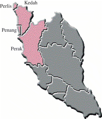
Peninsular Malaysia, with a total area of 131 598 km², is made up of 11 states and two federal territories, shares borders with Thailand and Singapore, and is bounded by the South China Sea and the Strait of Malacca. Located at 40′N–102°30′E, the whole Peninsula has an equatorial climate with temperatures ranging between 25.5 and 33°C. The amount of rain is influenced by the southwest and northeast monsoons, making it dry and wet throughout the year. In this study, the annual maximum streamflows of northern Peninsular Malaysia—comprising the states of Perak, Perlis, Kedah and Penang—were analysed using L-moments and TL-moments (1,0). The data were provided for this study by the Department of Irrigation and Drainage, Ministry of Natural Resources and Environment, Malaysia. Only data sets with record lengths of 10 years or more of annual maximum streamflows were used in this study. Figure 2 shows a map of northern Peninsular Malaysia.

Fig. 2 Map showing northern Peninsular Malaysia.

Hosking and Wallis (1997) suggested that the convenient way to represent the L-moments of different distributions is the L-moments ratio diagram. Ratio diagrams have often been used as a means of diagnosing how well a distribution describes data in a sample (Wang 1997). Since the GPA distribution contains three unknown parameters, the distribution can be estimated by using sample estimates of location, scale and kurtosis. The kurtosis that has been calculated directly from a sample can then be compared with the kurtosis of the estimated distribution. If the two are not statistically different, the distribution function can be regarded as describing the data well.

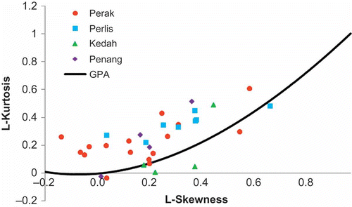
Figure 3 shows the L-moments diagram of skewness and kurtosis for streamflows of northern Peninsular Malaysia. A theoretical curve for the GPA distribution is also plotted in the diagram. Most of the sample estimates are located on the upper part of the theoretical GPA curve. Since TL-moments (1,0) reflect the characteristics of the upper part of the distribution more than L-moments, the former can be used to check whether larger events in a sample are well described by a particular distribution.

Fig. 3 L-moments diagram for annual maximum stream flows of northern Peninsular Malaysia.

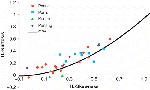
Figure 4 shows the TL-moments (1,0) ratio diagram for the same streamflow data. The kurtosis estimates are seen to scatter more evenly than L-moments on the theoretical GPA curve. This suggests that GPA distribution describes TL-moments (1,0) ratios better than L-moments ratios with respect to this data set.

Fig. 4 TL-moments (1,0) diagram for annual maximum stream flows of northern Peninsular Malaysia.

CONCLUSIONS

There has been insufficient discussion about the choice of trimming values in the paper by Elamir and Seheult (2003). Based on a few studies, we propose TL-moments where one smallest value is trimmed from the conceptual sample: TL-moments (1,0). The TL-moments (1,0) approach can be used to characterize the upper part of distributions and larger events in a sample. Thus, the parameters of the distribution can be estimated by matching TL-moments (1,0) to their sample estimates. The estimation of the GPA distribution using TL-moments (1,0) has been formulated.

The analysis using Monte Carlo simulation shows that using TL-moments (1,0) reduces the probable influence of small events in the sample on the estimation of large return-period events. The results from fitting the GPA distribution to a generated sample from Monte Carlo simulation for known parent distribution shows that TL-moments (1,0) leads to a reduced bias, as k becomes positive. In every shape parameter k, TL-moments (1,0) almost always give smaller RMSE values for all quantiles and sample sizes.

For the case of unknown parent distribution, TL-moments (1,0) give a smaller bias than L-moments for all Wakeby distributions. However, TL-moments (1,0) lead to a poorer estimation of high quantiles in terms of RMSE values for WA3, WA5 and WA6 for small sample size. For a larger sample size, using TL-moments (1,0) gives larger RMSE values for WA3 and WA5 than using L-moments. A comparison of the ratio diagram of annual maximum streamflow data over stations in northern Peninsular Malaysia shows that the GPA distribution does not give a very good fit to the data for both L-moments and TL-moments (1,0), and suggests that some other distributions should be considered. However, if we compare the L-moments and TL-moments (1,0), GPA distribution describes the TL-moments (1,0) ratios better than the L-moments ratios with respect to this data set. The result shows that for some cases, TL-moments (1,0) is a better option compared to the L-moments method, especially in high quantile estimation.

Acknowledgements

The author thanks the referees for their constructive comments, which helped improve the manuscript. The authors are also grateful to J.R.M. Hosking for reviewing and providing useful comments and suggestions for this manuscript.

REFERENCES

- Abdul Moniem , I.B. 2007 . L-moments and TL-moments estimation for the exponential distribution . Far East Journal of Theoretical Statistics , 23 ( 1 ) : 51 – 61 .
- Abdul Moniem , I.B. 2009 . TL-moments and L-moments estimation for the Weibull distribution . Advances and Application in Statistics , 15 ( 1 ) : 83 – 99 .
- Abdul Moniem , I.B. and Selim , Y.M. 2010 . TL-Moments and L-Moments estimation for the generalized Pareto distribution . Applied Mathematical Sciences , 3 ( 1 ) : 43 – 52 .
- Asquith , W.H. 2007 . L-moments and TL-moments of the generalized lambda distribution . Computational Statistics and Data Analysis , 51 : 4484 – 4496 .
- Bhattarai , K.P. 2004 . Partial L-moments for the analysis of censored flood samples . Hydrological Sciences Journal , 49 ( 5 ) : 855 – 868 .
- Cunnane , C. 1987 . “ Review of statistical models for flood frequency estimation ” . In Hydrological frequency modelling , Edited by: Singh , V.P. 49 – 95 . Dordrecht : D. Reidel .
- Elamir , E.A.H. and Seheult , A.H. 2003 . Trimmed L-moments . Computational Statistics and Data Analysis , 43 : 299 – 314 .
- Hosking , J.R.M. 1990 . L-moments: analysis and estimation of distributions using linear combinations of order statistics . Journal of the Royal Statistical Society B , 52 : 105 – 124 .
- Hosking , J.R.M. 2007 . Some theory and practical uses of trimmed L-moments . Journal of Statistical Planning and Inference , 137 : 3024 – 3039 .
- Hosking , J.R.M. and Wallis , J.R. 1997 . Regional frequency analysis: An approach based on L-moments , Cambridge : Cambridge University Press .
- Houghton , J.C. 1978 . Birth of a parent: the Wakeby distribution for modelling flood flows . Water Resources Research , 14 ( 6 ) : 1105 – 1110 .
- Landwehr , J.M. , Matalas , N.C. and Wallis , J.R. 1980 . Quantile estimation with more or less floodlike distributions . Water Resources Research , 16 ( 3 ) : 547 – 555 .
- Saf , B. 2008 . Regional flood frequency analysis using L-moments for the west Mediterranean region of Turkey . Water Resources Management , 23 : 531 – 551 .
- Stedinger , J.R. , Vogel , R.M. and Foufoula-Georgiou , E. 1992 . “ Frequency analysis of extreme events ” . In Handbook of hydrology , Edited by: Maidment , D.R. New York : McGraw-Hill . Chapter 18
- Vogel , R.M. and Fennessey , N.M. 1993 . L-moments diagrams should replace product moment diagrams . Water Resources Research , 29 ( 6 ) : 1745 – 1752 .
- Wang , Q.J. 1990 . Estimation of the GEV distribution from censored samples by method of partial probability weighted moments . Journal of Hydrology , 120 ( 1–4 ) : 103 – 114 .
- Wang , Q.J. 1997 . LH-Moments for statistical analysis of extreme events . Water Resources Research , 33 ( 12 ) : 2841 – 2848 .