Probabilistic flood forecasting for a mountainous headwater catchment using a nonparametric stochastic dynamic approach

Abstract

Hydrological models are commonly used to perform real-time runoff forecasting for flood warning. Their application requires catchment characteristics and precipitation series that are not always available. An alternative approach is nonparametric modelling based only on runoff series. However, the following questions arise: Can nonparametric models show reliable forecasting? Can they perform as reliably as hydrological models? We performed probabilistic forecasting one, two and three hours ahead for a runoff series, with the aim of ascribing a probability density function to predicted discharge using time series analysis based on stochastic dynamics theory. The derived dynamic terms were compared to a hydrological model, LARSIM. Our procedure was able to forecast within 95% confidence interval 1-, 2- and 3-h ahead discharge probability functions with about 1.40 m³/s of range and relative errors (%) in the range [–30; 30]. The LARSIM model and the best nonparametric approaches gave similar results, but the range of relative errors was larger for the nonparametric approaches.

Editor D. Koutsoyiannis; Associate editor K. Hamed

Citation Costa, A.C., Bronstert, A. and Kneis, D., 2012. Probabilistic flood forecasting for a mountainous headwater catchment using a nonparametric stochastic dynamic approach. Hydrological Sciences Journal, 57 (1), 10–25.

Résumé

Les modèles hydrologiques sont couramment utilisés pour effectuer la prévision de l'écoulement en temps réel pour les alertes de crues. Leur application requiert des caractéristiques des bassins versants et la série des précipitations qui ne sont pas toujours disponibles. Une approche alternative est la modélisation paramétrique basée uniquement sur les séries d'écoulement. Cependant, les questions suivantes se posent: les modèles non paramétriques peuvent-ils produire des prévisions fiables? Peuvent-ils être utilisés de manière aussi fiable que les modèles hydrologiques? Nous avons effectué des prévisions probabilistes d'une chronique d'écoulement aux horizons d'une, deux et trois heures, dans le but d'attribuer une fonction densité de probabilité aux prévisions de débits en utilisant l'analyse de séries chronologiques basée sur la théorie de la dynamique stochastique. Les termes dynamiques dérivés ont été comparés au modèle hydrologique LARSIM. Notre procédure a permis de prévoir les fonctions de probabilité du débit 1, 2 et 3 heures à l'avance dans l'intervalle de confiance à 95%, avec un écart d'environ 1,40 m³/s, et des erreurs relatives (en %) dans l'intervalle [–30 ; 30]. Le modèle LARSIM et les meilleures approches non paramétriques ont fourni des résultats similaires, mais l'éventail des erreurs relatives s'est révélé plus important pour les approches non paramétriques.

Key words:

• streamflow probabilistic forecasting
• time series analysis
• stochastic dynamical systems
• parametric and nonparametric comparison

Mots clefs:

• prévision probabilistes des débits
• analyse des séries chronologiques
• systèmes dynamiques stochastiques
• comparaison paramétriques et non paramétriques

INTRODUCTION

Hydrologists commonly use distributed hydrological models to perform real-time streamflow forecasting for flood warning purposes. These models require large data sets of catchment physical characteristics and precipitation series that are not always available. Furthermore, the results from these models can be rather uncertain due to large errors in precipitation input, initial catchment moisture conditions and/or modelling parameters/processes. An alternative approach is to use nonparametric models based on streamflow series only, to overcome the requirement for data on catchment physical characteristics and precipitation series. However, it is not known whether nonparametric models for meso-scale catchments can show reliable streamflow forecasting for flood warning, or whether they can perform as reliably as, or even outperform, distributed hydrological models.

Since the beginning of the 1990s, runoff series have been assumed as responses of dynamical systems with a low-dimensional chaotic attractor resulting from the nonlinear coupling of precipitation and catchment state that depends on climatic condition and geo-patterns, such as land cover, soils, river network and geology (Liu et al. 1998, Porporato and Ridolfi 1997, Sivakumar et al. 2001). A fundamental characteristic of a dynamical system is that it returns or recurs to former states (recurrence) (see discussion in Marwan et al. 2007).

This assumption means that the “catchment-runoff-system” should obey a deterministic operator, a set of coupling ordinary differential equations of the involved variables (e.g. runoff, precipitation and soil moisture). This operator projects a trajectory in the state space (or phase space), which establishes all states of the involved variables. The catchment runoff system states return or recur to former states during their trajectory in the state space. However, recently, the hypothesis that hydrological processes are governed by dynamics with low-dimensional attractors has been disputed e.g. in Koutsoyiannis (2006).

In this context, chaotic systems theory has been applied to hourly, daily and monthly runoff series employing nonparametric models by the phase space reconstruction technique (Jayawardena and Lai 1994, Liu et al. 1998, Jayawardena and Gurung 2000, Sivakumar et al. 2001, Porporato and Ridolfi 1997, 2001, Sivakumar et al. 2002, Laio et al. 2003). Moreover, even without a low-dimensional chaotic attractor, this nonlinear dynamics approach can also give good predictions (Koutsoyiannis et al. 2008).

This nonlinear approach can provide accurate one-discharge-value-per-time-step forecasting, but it does not always offer insight into the probabilistic structure of the data resulting from the shortness of series, and the inevitable presence of dynamical noise in open physical systems, such as catchment runoff (Porporato and Ridolfi 2001, Kantz and Schreiber 2004). Moreover, the ability of the nonlinear approach to give information on uncertainties associated with forecasts is limited (Komorník et al. 2006), and this is central to the implementation of effective flood warning or flood protection measures (see Todini 2004). To address the last issue, Tamea et al. (2005) proposed: (a) an ensemble-based nonlinear prediction with parametric deterministic range similar to the GLUE method (Beven and Binley 1992, Beven 1993); and (b) a probabilistic prediction using global errors of a training set to “dress” the deterministic forecasts, which was also done by Chen and Yu (2007) using support vector machine background.

In this paper, we deal with real-time probabilistic forecasting of river discharge. For this task, we apply stochastic dynamics theory related to time series analysis in hydrology to deal with both deterministic evolution and inherent fluctuations in river discharge data. In this way, we consider a dynamical system (autonomous set of deterministic equations), such as the Lorenz equations, contaminated by external noise (van Kampen 1992, Anishenko et al. 2003, Kantz and Schreiber 2004), as the driving physical assumption for catchment runoff.

A stochastic dynamical system can be expressed mathematically by time series models, where the dynamic or deterministic part is approached by a regression model and the stochastic part by noise, which does not depend on the states of the dynamic part.

The objectives of this work are to perform one-, two- and three-hour ahead probabilistic forecasting for runoff series, i.e. to ascribe a probability density function (pdf) to predicted discharge, in a mountainous headwater catchment (49 km²) using time series models. Furthermore, the deterministic evolution of the time series models will be compared to a comprehensive hydrological model called LARSIM, which has been used for operational forecasts of floods, low flow and water temperature in Germany (Ludwig and Bremicker 2006).

In this way, we intend to identify an underlying dynamical system for a noisy runoff series and approach it by a proposed nonparametric stochastic dynamic model.

Identifying a dynamical system for catchment runoff means that a similar flood magnitude will be expected for an actual set of catchment runoff states similar to a previous one (determinism). This deterministic paradigm is quite different, if we assume a random nature of the data and then apply time series models, which has been done using nonparametric stochastic forecasting approaches only.

NONPARAMETRIC MODELLING

Dynamical systems

A dynamical system may be thought as a set of variables x (x ¹, x ², … , xⁿ ), whose states are observed in time t as simply a result of the action of a deterministic evolution operator that does not depend on t, in some state space Rⁿ . Once a state is known, the states of all surroundings are determined as well by:

(1)

The value of a variable specifies a point in state space, and vice versa. Hence, one can approach the deterministic evolution operator by the dynamics of values of a unique variable, which is called phase space or delay reconstruction (see Anishchenko et al. 2003, Kantz and Schreiber 2004).

Considering x _t in Rⁿ , the delay reconstruction of x_t can be written based on Takens (1980) as:

(2)

As an example we consider the Lorenz equations (Lorenz 1963):

(3)

We integrated equation (3)(3) using a Runge-Kutta routine with small step size. Then, we plotted their two-dimensional (2D) evolution (x_t vs y_t variables) in Fig. 1(a) and their reconstructed 2D evolution (x_t vs x_{t -8} variables) in Fig. 1(b).

Fig. 1 (a) Two-dimensional evolution (x_t vs y_t variables); and (b) reconstructed 2D evolution (x_t vs x_{t -8} variables) of Lorentz equations.

Thus, the evolution of a dynamical system is “printed” on the past observations of a unique variable of it. Now, suppose a time series of a variable of the dynamical system x _t ; it is validated from equations (1)(1) and (2) that:

(4)

If one aims to predict x_t using the map (4), it can be modelled by a regression model, where a forecast state is estimated by the values of the variable at n past steps. This needs a short-range dependence of the time series, that is, its autocorrelation function (acf) c_{j .Δt} in relation to a step Δt has to reach approximately zero at a short shift K (based on Koutsoyiannis et al. 2008):

(5)

where l is the total number of events, j and K are non-zero natural numbers. However, as pointed out by Fisher (1928), the variance s² _c,l of the empirical coefficient of correlation c_{K .Δt} follows:

(6)

Then, for a finite sample, Fisher's interval [–s_c,l ;s_c,l ] limits the region around the acf's zero, where the uncorrelated behaviour of its acf cannot be rejected.

Furthermore, the n past steps can be approximated by the (K – 1) neighbours with coefficient of correlation greater than s_c,l (see also Fig. 2) as:

(7)

Fig. 2 Autocorrelation functions (acfs) of: (a) uniformly-distributed noise, (b) a sine function (periodic motion), and (c) the x variable of the Lorenz equations.

Probabilistic approach

Our main point in this paper is that the determinism is broken up due to the presence of fluctuations in open physical systems like catchment runoff. Therefore, we add a global stochastic term on the map (7), modifying it to:

(8)

where ξ could be white or coloured noise. Adopting an a priori regression model to F, we can afterwards estimate the distribution of ξ from a training set, diminishing the training set measurement X_ts and prediction of the dynamic term F. Then, we can define different confidence intervals, e.g. 90 and 95%, for the distribution of ξ as a histogram with zero mean. Note that x_i has to be normalized to a pdf with zero mean and standard deviation equal to one.

Using the relationship (8), the expected value of _η is predicted by F (dynamic term) and its uncertainty by the distribution of ξ (stochastic term) with a confidence interval, ascribing in this manner a pdf for _η.

When measurements in a validation set occur outside the limits of the confidence intervals of the pdf given by equation (8)(8), [F + ξ⁻; F + ξ⁺], we achieve the validation set error ϵ, defined as:

(9)

where x_v is measurement in a validation set. Note that the distribution of ξ includes the uncertainty not only from the inherent fluctuations of the runoff data, but also from the fitting of the underlying dynamic term by an assumed regression model.

The probabilistic approach presented in this section is quite similar to the probabilistic forecast method found in Tamea et al. (2005). However, our approach simplifies the Tamea et al. (2005) method, which needs many realizations of the forecast error and calibration of a correction term for the distribution of the residuals.

Regression models

Several authors (Jayawardena and Lai 1994, Liu et al. 1998, Jayawardena and Gurung 2000, Sivakumar et al. 2001, Porporato and Ridolfi 1997, 2001, Sivakumar et al. 2002, Laio et al. 2003) have presented cases in which local approaches, i.e. locally fitted models, have outperformed nonlinear and linear global ones, although Koutsoyiannis et al. (2008) presented a case in which a global stochastic model outperformed a locally-fitted and a global nonlinear approach.

In this method, we adopt regression models that are: (a) locally averaged, whose only unknown parameter is the number of neighbourhoods (n past steps), and (b) locally constant, in that the predicted value is assumed to be equal to the last measurement.

We also use the autoregressive model (AR), whose unknown parameters are the number of neighbourhoods and its coefficients from an acf, for the dynamic term F as reference to test the hypothesis of linear random data. Note that we do not apply an ARMA, because the noise inputs of the moving average model (MA) are not known before the application of equation (8)(8) and must be averaged. This was also done by Kantz and Schreiber (2004) applying nonlinear methods only.

Identifying dynamical systems from noisy time series

Before the application of equation (8)(8), we must identify experimentally whether a dynamical system can be assumed from a given noisy runoff series.

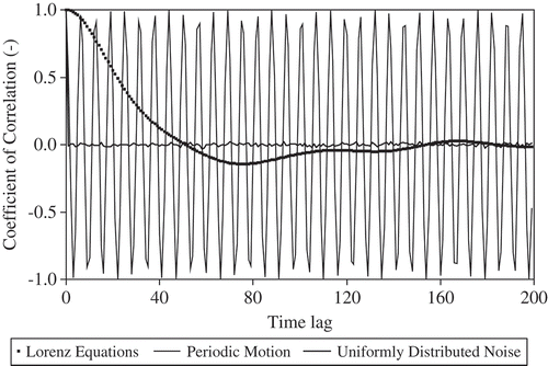
The identification of dynamical systems by nonlinear methods (e.g. correlation or entropy dimensions) requires a large amount of noise-free data (Kantz and Schreiber 2004). Therefore, we use autocorrelation functions (acfs) to identify qualitatively dynamical systems from very noisy time series. In this section, we compare the acfs of: (a) uniformly-distributed noise, (b) a sine function (periodic motion), and (c) the x variable of the Lorenz equations. The acfs of these three systems are plotted in Fig. 2.

Figure 2 shows that the acf of a dynamical system decays exponentially to zero and then oscillates quasi-periodically around zero, whereas that of uniformly-distributed noise has small fluctuations around zero. The acf of the periodic motion only reflects its “periodicity”.

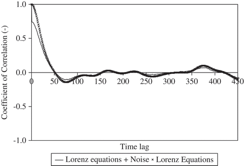
Now, if we include external uniformly-distributed noise into the time series of the x variable of the Lorenz equations (Fig. 3), the acf of the new noisy system decays rapidly at the initial time lags and then exponentially to zero. After the time lag equal to 50, it oscillates quasi-periodically around zero with lower correlation compared to the noise-free acf.

Fig. 3 Autocorrelation functions of the x variable of the Lorenz equations with and without uniformly-distributed noise.

PARAMETRIC MODELLING

In this study, we compare the presented nonparametric modelling to a comprehensive hydrological model called LARSIM, which has been used for operational forecasts of floods, low flow and water temperature in Germany (Ludwig and Bremicker 2006). LARSIM is a distributed hydrological model, which distinguishes most relevant hydrological processes such as interception, evapotranspiration, snow accumulation, snow compaction and snowmelt, soil water storage and water flow and storage in streams and lakes (Ludwig and Bremicker 2006). It can apply a raster-based spatial discretization for easy usage of routinely available physical catchment data (e.g. slope, land use and field capacity) and hydro-meteorological time series (Ludwig and Bremicker 2006).

AN EXAMPLE OF PROBABILISTIC FLOOD PREDICTION

Data overview

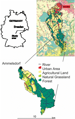
The time series analysis was carried out for Ammelsdorf streamgauge, which limits a catchment of about 49 km² located in the eastern Ore Mountains, Germany, close to the Czech–German border (Fig. 4). About 2 km downstream of this gauge is the artificial reservoir Lehnmühle, which dampens or adjusts the river discharge, particularly during flood events. According to Reusser et al. (2009) and Bronstert et al. (2011), the catchment has an elevation of 530 to about 900 m a.s.l and slopes are gentle, with an average of 7°. The climate is moderate with mean temperatures of 11°C and 1°C for the periods April–September and October–March, respectively, and annual precipitation is about 1100 mm/year. High flows can be induced by either convective rainfall during the summer or snowmelt in spring. Land use is characterized by forests (58.3%), natural grassland (20.1%), agriculture (9.6%), pasture (6.1%), peat bog (3.7%) and urban areas (2.2%).

Fig. 4 Location of the Weisseritz headwater catchment, upstream of the Ammelsdorf streamgauge's catchment.

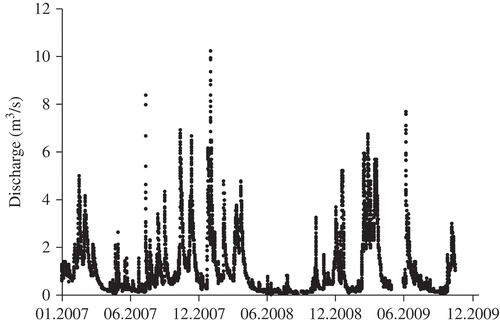
Discharge data were obtained from the Saxony state office for environment and geology. Discharge data for the Ammelsdorf streamgauge were made available hourly and the series runs from January 2000 to October 2009. The average discharge was 1.01 m³/s and the coefficient of variation was 1.5, with 0.04 and 35.44 m³/s being the minimum and maximum measured discharge, respectively. The discharge series for 2007–2009 is shown as an example in Fig. 5.

Fig. 5 Hourly discharge series for the Ammelsdorf streamgauge for 2007–2009.

Runoff nonparametric modelling

Identifying an underlying dynamical system

Previous works on nonparametric discharge forecasting (Jayawardena and Lai 1994, Liu et al. 1998, Jayawardena and Gurung 2000, Sivakumar et al. 2001, Porporato and Ridolfi 1997, 2001, Sivakumar et al. 2002, Laio et al. 2003, Tamea et al. 2005) have used the discharge time series as the independent variable, but if its autocorrelation function does not reach the uncorrelated behaviour (short-range dependence), even if the time series are driven by a dynamical system, we should not fit a regression model to the dynamic term F in equation (8)(8).

We calculated here the autocorrelation function (acf) for the discharge time series (Q) and also for its first (Q′) and second (Q′′) time derivatives (Fig. 6) to find out whether a dynamical system can be assumed in a qualitative way from our original time series.

Fig. 6 Autocorrelation function of the hourly discharge series (Q) and of its first (Q′) and second (Q′′) time derivatives for the Ammelsdorf streamgauge (2000–2009 with gaps), Fisher's interval limits indicating the uncorrelated behaviour that cannot be rejected.

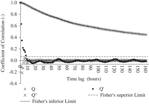
Figure 6 shows that the discharge time series did not exhibit a short-range dependence, rather it exhibited a long-range dependence (i.e. power-type decay of autocorrelation also known as the Hurst phenomenon e.g. Koutsoyiannis 2002), and, consequently, we should not use these time series for regression model-based approaches. The second derivative of discharge series for a time lag equal to 4 h reached the uncorrelated behaviour, but its acf is similar to that of noise systems, showing its very low predictability. However, the first derivative of discharge series exhibited a short-range dependence and its acf presented a structure similar to that of dynamical systems contaminated with noise, i.e. a rapid decay in the initial time lags and then exponential decay to zero. After a time lag of about 7 h, it oscillates quasi-periodically around zero. Consequently, we used the first derivative of discharge time series to forecast the original discharge time series.

One-, two- and three-hour ahead probabilistic prediction

The hourly first time derivative of discharge time series was re-sampled to also create two- and three-hour series by applying:

(10)

where Q_t is the original discharge time series and i is t + Δt/2. The time interval Δt was set as 1, 2 and 3 h.

We then multiplied the first time derivative of runoff, equation (10)(10), by its time interval for all the one-, two- and three-hour time series, defining in this way the difference between two runoff measurements—the runoff difference—as the independent variable in this study.

Applying equation (8)(8), probabilistic predictions of runoff differences in m³/s for one time interval Δt ahead were carried out for one-, two- and three-hour time series using:

(11)

We considered three approaches for the dynamic term F: (a) an autoregressive model, (b) a locally averaged model, and (c) a locally constant model. The term ξ was defined previously. Afterwards, the prediction of runoff differences for one-, two- and three-hour time series was used in equation (12)(12) below to achieve the probabilistic prediction of stream discharges for 1, 2 and 3 h ahead:

(12)

where Q_t is the measured stream discharge and is the predicted probability function of stream discharge. Note that stream discharge assimilation is taken in account by equation (12)(12).

Runoff events filter

The procedure described in the last section was only applied for what we called runoff events of the time series. Given a series of runoff differences , we defined a runoff event within it when continuous measurements obey: (a) or (b) , if and . In addition, only the runoff events with duration greater than 6 h were taken into account to avoid trends in fitting of the autoregressive model and the locally averaged model due to a large quantity of small runoff events in the time series.

Performance criterion

As an error measure we used relative error, RE (in %; equation (13)(13)), to assess the differences between runoff measurements (m³/s) and the confidence interval limits of the predicted pdfs of equation (11)(11):

(13)

where ϵ was defined as in equation (9)(9). To ease the derivation of equation (13)(13), the range-based formulation of ϵ was not taken into account here. As this work is intended to forecast probabilistic streamflow for flood warning purposes, the best approach for a given confidence interval of the probability distribution of ξ in equation (12)(12) minimizes the range of ξ and relative error (RE).

Results

Nonparametric forecasting

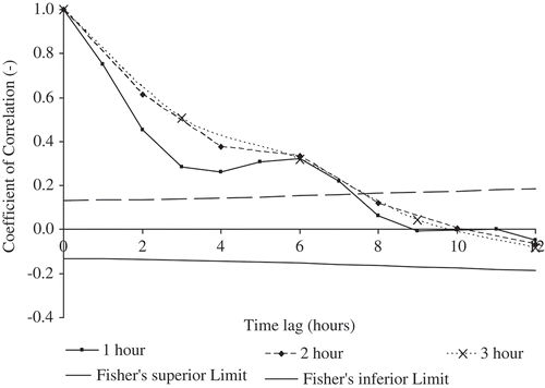
Adopting the first 75% of the runoff series as a training set, we calculated the pdfs (Fig. 7) and the partial autocorrelation functions (acfs) (Fig. 8) for one-, two- and three-hour time series.

Fig. 7 Probability density function of the hourly differences between two runoff measurements, runoff differences, using the first 75% of the runoff differences as the training set.

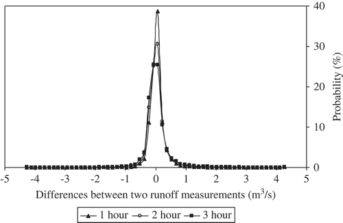
Fig. 8 Partial autocorrelation function of the hourly differences between two runoff measurements, runoff differences, using the first 75% of the runoff differences as the training set, Fisher's interval limits indicating the region where the uncorrelated behaviour cannot be rejected.

Because of the runoff events filter, the following statistics and the coefficients of partial acfs changed for one-, two- and three-hour time series (Fig. 8). The pdfs of in-training set runoff differences for one-, two- and three-hour time series were approximately similar to a Gaussian distribution. The most runoff differences were in narrow ranges. Runoff differences larger than 2.1 m³/s showed 0.2, 0.4 and 0.8% probability for one-, two- and three-hour time series, respectively. The mean and the standard deviation are 0.04 and 0.33, 0.03 and 0.48, 0.03 and 0.58 m³/s for one-, two- and three-hour time series, respectively.

Comparing the mean and standard deviation of training and validation sets for one-, two- and three hour time series, we found that the means of both sets were practically the same, but the standard deviation of the validation set is about 33% smaller than that of the training set. This means that the data variability of the validation set is not a source of uncertainty for forecasting results.

The runoff differences whose coefficients of correlation of the partial acfs were greater than Fisher's superior limit were adopted as neighbourhoods in time for both autoregressive and locally averaged model-based approaches, and their coefficients of correlation for autoregressive models. After a normalization of stream discharge data, we applied autoregressive, locally averaged and locally constant model-based approaches to the training set. We had the following dimensionless time series models for one-, two- and three-hour time series (Table 1). Note that we had to diminish the mean <ξ> of the distribution ξ to achieve a histogram with zero-mean as stochastic term.

Table 1  Dynamic and stochastic terms of time series models (dimensionless), adopting autoregressive (AR), locally averaged and locally constant models as approaches for the dynamic term F

F	<ξ>	Distribution of (ξ – <ξ>)
		1 hour
AR(7)	0.17
	0.13
	0.40
		2 hour
AR(3)	0.04
	0.04
	0.01
		3 hour
AR(2)	0.04
	0.05
	0.04

It can be seen from Table 1 that the distributions of (ξ – <ξ>) (the stochastic part of equation (8)(8)) were in narrow ranges, approximately similar to a Gaussian distribution, for one-, two- and three-hour time series, excluding only the AR(7)-based distribution. The sharpest distribution for one- and two-hour time series was the locally averaged model-based one; in contrast, the sharpest distribution for three-hour time series was the autoregressive model-based one.

After the derivation of these approaches, we applied them and computed the range of relative errors considering 97.5, 95 and 90% confidence intervals of the distribution of (ξ – <ξ>) for one-, two- and three-hour time series. For this calculation, we used not only the last 25% of the runoff differences, but also the training set as well, because it presented high runoff differences with low probability (see above in this section), which can generate, for instance, high relative errors.

We adopted absolute relative errors (see equation (13)(13)) about smaller than 30% with 90% confidence interval as the criterion of reliability for stream discharge forecasting. In this manner, we found from previous investigation that reliable forecasting was produced only when measured stream discharges, Q_t were: (a) higher than 5.5 m³/s for one-hour time series, and (b) higher than 8.8 m³/s for two- and three-hour time series. Note that reliability is subjective and these discharge thresholds can vary between applications.

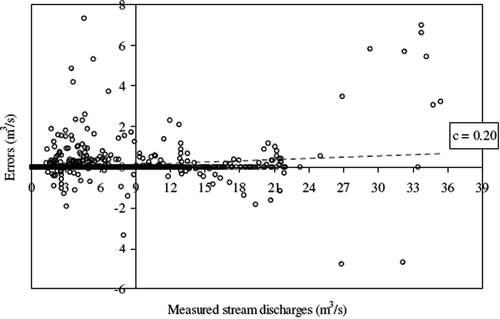
The above discharge thresholds can be explained by equation (13)(13), whereby the higher the measured stream discharges, the smaller the relative errors. Nevertheless, although one could argue that from a certain discharge threshold the errors could be smaller, no statistical evidence of this trend was found in the time series (e.g. Fig. 9 shows measured stream discharges vs errors from the application of the autoregressive approach to two-hour time series with 95% confidence interval).

Fig. 9 Measured stream discharges vs errors from the application of autoregressive approach to two-hour time series with 95% confidence interval, where c is the coefficient of correlation.

We carried out further performance analysis of the nonparametric models, considering discharge threshold levels for one-, two-, and three-hour time series (see Table 2). Hence, the number of predicted stream discharges for one-, two- and three-hour time series, respectively, was 516, 300 and 347.

Table 2  Performance of autoregressive (AR), locally averaged and locally constant model-based approaches for 97.5, 95 and 90% confidence intervals of the distributions of (ξ – <ξ>) (m³/s) in one-, two- and three-hour time series, where relative error, RE (in %) is related to the differences between runoff measurements (m³/s) and confidence interval limits of the predicted probability density functions (equation (13)(13)). These results are only valid for certain discharge threshold levels (5.5 m³/s for one-hour time series, and 8.8 m³/s for two- and three-hour time series)

Approach	Stochastic terms	1 h, p = 7			2 h, p = 3			3 h, p = 2
		97.5%	95%	90%	97.5%	95%	90%	97.5%	95%	90%
AR [p]	Range length of (ξ – <ξ>)	2.94	2.14	1.60	2.52	1.84	1.21	2.20	1.50	0.98
	Range interval of RE	[−11; 38]	[−12; 46]	[−13; 50]	[−16; 20]	[−18; 21]	[−19; 23]	[−31; 30]	[−32; 31]	[−33; 33]
Locally averaged [p]	Range length of (ξ – <ξ>)	1.74	1.20	0.74	1.89	1.45	0.92	2.66	1.85	1.16
	Range interval of RE	[−10; 27]	[−12; 30]	[−13; 32]	[−20; 19]	[−21; 20]	[−22; 22]	[−28; 32]	[−30; 36]	[−31; 40]
Locally constant	Range length of (ξ – <ξ>)	1.00	0.74	0.53	2.04	1.36	0.92	2.83	1.85	1.16
	Range interval of RE	[−8; 34]	[−8; 35]	[−9; 36]	[−21; 24]	[−23; 25]	[−24; 25]	[−28; 35]	[−30; 40]	[−32; 43]

As the best approach minimizes the range of (ξ – <ξ>) and relative error, RE, we tried to find an optimum among these criteria to choose the best approach for each confidence interval in each time series. In this way we found from Table 2 that the locally averaged model-based approach was the best for one- and two-hour time series and the autoregressive approach for three-hour time series.

Now, taking a look at the largest runoff events, we chose the largest runoff events in both validation and training sets. The analysis of the training set event was carried out because it was the largest event in the discharge time series, showing 35.44 m³/s of peak runoff and high runoff differences with low probability. We used the best chosen approaches with 95% confidence interval for 1-, 2- and 3-h ahead probabilistic runoff forecasting of these events. Figure 10(a)–(c) shows the results of validation set prediction and Fig. 11(a)–(c) that for the training set.

Fig. 10 Probabilistic runoff forecasting of the largest runoff event in the validation set for: (a) 1 h ahead, (b) 2 h ahead and (c) 3 h ahead, with 95% confidence interval, corresponding to differences (between upper and lower predicted runoff) of 1.20, 1.45 and 1.50 m³/s, respectively.

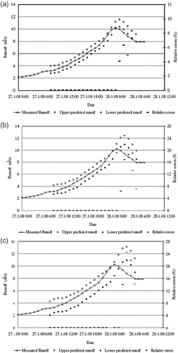
Fig. 11 Probabilistic runoff forecasting of the largest runoff event in the training set for: (a) 1 h ahead, (b) 2 h ahead, and (c) 3 h ahead, with 95% confidence interval, corresponding to differences (between upper and lower predicted runoff) of 1.20, 1.45 and 1.50 m³/s, respectively.

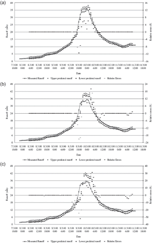
Figures 10 and 11 show that the measured rising limb and falling limb of the largest runoff events in the validation and training sets were almost within the predicted runoff ranges for the three time series. However, overestimation of peak flow was not negligible for two- and three-hour events (Figs 10(b), 10(c), 11(b) and 11(c)), and one high runoff underestimation (about –30%) in the rising limb was observed in the three-hour ahead, largest event of the training set (Fig. 11(c)).

It is also important to evaluate whether measurements of runoff differences ΔQ_{i, Δt} and validation set residuals were systematic, because, if they were, it means that part of the determinism was not identified by modelling (Kantz and Schreiber 2004). Considering the best approaches for one-, two- and three-hour time series, we plotted validation set residuals vs measurements of runoff differences in Fig. 12(a)–(c) and computed their coefficients of correlation and Fisher's limits.

Fig. 12 Measurements of runoff differences vs validation set residuals, considering the best approaches for: (a) hourly time series, (b) two-hour time series, and (c) three-hour time series, where c is the coefficient of correlation.

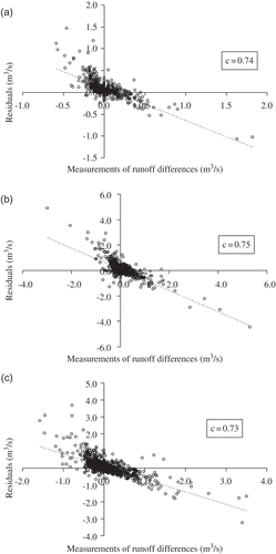
Since the coefficients of correlation were greater than its Fisher's superior limits, a negative linear relation could not be rejected between validation set residuals and measurements of runoff differences for the time series. Also insights into location of measured discharges on predicted probability density functions are possible, but at this moment this analysis is outside the scope of this work and will be investigated later.

Comparison with the forecast obtained by a comprehensive hydrological model

In this section we compare the results of used nonparametric models with the ones obtained by a comprehensive hydrological model LARSIM (see Section PARAMETRIC MODELLING). The description of parameterization and input variables of LARSIM model to a meso-scale catchment can be found in Heistermann and Kneis (2011). LARSIM was applied to the Ammelsdorf gauge catchment independently.

An hourly forecasting using LARSIM for the Ammelsdorf gauge with stream discharge assimilation, i.e. in “prediction mode”, consumes too much computer time and is hardly feasible.

Therefore, the following alternative was formulated: (a) to apply hourly LARSIM without stream discharge assimilation and any kind of corrections to model states and parameters at intermediate times, i.e. in “simulation mode”, (b) then to use the relationship

(14)

where and are stream discharge simulated by LARSIM without stream discharge assimilation or any kind of correction to the model states and parameters at intermediate times; Q_t is the measured stream discharge; and is the predicted stream discharge.

The simulation mode is worse than the prediction mode for operational stream discharge forecasting, but equation (14)(14) has the advantage of not compromising any model uncertainties on stream discharge assimilation.

Furthermore, in a previous investigation on hourly hydrographs and areal hyetographs, it was found that an average catchment reaction time was between 3 and 5 hours. Thus only the observed precipitation was adopted as LARSIM input to forecast one-, two- and three-hour ahead stream discharge.

The application of LARSIM to the Ammelsdorf gauge was carried out from a deterministic point of view only, i.e. one-discharge-value-per-time-step forecasting, and, consequently, we were only able to compare the dynamic terms of the nonparametric approaches with LARSIM's results. We used the common calibration set results of both applications (parametric and nonparametric) from May 2004–January 2008 as the compared set, because it was quite a bit larger than the common validation set results. The mean absolute error, MAE (in %) and the range of relative errors, RE (in %) (see equation (13)(13)) were considered as criteria of goodness of fit. Table 3 shows the comparison for one-, two- and three-hour time series according to the size of the measured discharge (m³/s).

Table 3  Comparison of LARSIM application and the dynamic terms of the nonparametric models—autoregressive (AR), locally averaged and locally constant model-based approaches—for one-, two- and three-hour time series. The number of compared samples, mean absolute error, MAE (in %) and the range of relative errors, RE (in %) are given according to the amount of measured discharge (m³/s)

Measured discharge (m^3/s) higher than	Number of compared samples	LARSIM application		AR		Locally averaged		Locally constant
		MAE	Range of RE	MAE	Range of RE	MAE	Range of RE	MAE	Range of RE
1 hour
0.0	892	4.3	[−38; 55]	10.2	[−85; 79]	6.5	[−47; 52]	5.3	[−51; 96]
1.1	762	3.5	[−38; 26]	9.5	[−85; 61]	5.5	[−47; 52]	3.8	[−40; 39]
2.2	596	2.8	[−38; 26]	7.8	[−58; 61]	4.5	[−42; 52]	3.0	[−33; 39]
4.4	391	2.2	[−38; 26]	6.2	[−21; 61]	3.0	[−38; 38]	2.3	[−26; 39]
6.6	218	1.8	[−38; 26]	5.8	[−21; 61]	2.2	[−38; 38]	1.9	[−26; 39]
2 hour
0.0	2004	7.4	[−67; 376]	11.3	[−101; 177]	10.5	[−96; 159]	10.0	[−100; 203]
1.1	1471	5.4	[−67; 76]	9.4	[−101; 177]	8.6	[−96; 159]	7.6	[−100; 203]
2.2	1045	4.3	[−67; 76]	7.8	[−98; 177]	7.3	[−96; 159]	6.2	[−100; 203]
4.4	639	3.2	[−48.7; 76]	5.5	[−55; 177]	4.8	[−56; 141]	4.4	[−62; 203]
6.6	300	2.9	[−48.7; 25]	4.5	[−55; 67]	3.8	[−56; 45]	3.2	[−62; 99]
3 hour
0.0	2945	8.9	[−63; 407]	12.6	[−97; 259]	13.7	[−140; 258]	13.6	[−161; 370]
1.1	2111	6.2	[−63; 118]	9.7	[−97; 259]	10.9	[−140; 258]	10.4	[−161; 370]
2.2	1523	5.0	[−63; 118]	8.2	[−97; 259]	9.2	[−97; 258]	8.6	[−161; 370]
4.4	753	3.9	[−51; 75]	6.1	[−70; 144]	6.6	[−69; 144]	6.3	[−86; 207]
6.6	349	3.8	[−51; 14]	5.2	[−69; 32]	5.7	[−62; 35]	5.0	[−86; 39]

It was observed in general that the higher the measured discharge, the smaller the MAE and the range of RE of all approaches. The MAE of the LARSIM application was slightly smaller than the best results of the nonparametric approaches; however, the nonparametric approaches always showed larger ranges of RE for measured discharges higher than 1.1 m³/s, independently of the lead time of forecast.

DISCUSSION AND CONCLUSIONS

We have developed in this paper a nonparametric, stochastic dynamic procedure, which used a qualitative dynamical system-based decision criterion for discharge time series forecasting and dealt with the probabilistic nature of the river discharge data. This approach was based only on the discharge time series itself and needed little computation time.

We assessed our procedure for a meso-scale catchment (about 49 km²), in which runoff events are induced by either convective rainfall during the summer or snowmelt in spring, and ascribed probability density functions to 1-, 2- and 3-h ahead predicted discharge.

Instead of the actual runoff measurements (Jayawardena and Lai 1994, Liu et al. 1998, Jayawardena and Gurung 2000, Sivakumar et al. 2001, Porporato and Ridolfi 1997, 2001, Sivakumar et al. 2002, Laio et al. 2003, Tamea et al. 2005), the differences between the runoff measurements were used for application of the regression models, because the last series exhibited short-range dependence and presented similar structure to that of dynamical systems contaminated with noise.

The best approaches for one-, two- and three-hour ahead discharge time series were those, which have the sharpest probability density functions for the stochastic term. The locally averaged model-based approaches were the best ones for one- and two-hour time series and the autoregressive model was the best one for the three-hour time series.

This means that the system shifted from a possible dynamical system contaminated with noise to a linear random process, when the interval time of time series increased. This is expected even for noise-free dynamical systems (see Kantz and Schreiber 2004). Therefore, we did not find in this work a best unique formulation among the three assumed approaches (autoregressive model, locally averaged and locally constant models) for the dynamic term, although previous studies (Jayawardena and Lai 1994, Liu et al. 1998, Jayawardena and Gurung 2000, Sivakumar et al. 2001, Porporato and Ridolfi 1997, Sivakumar et al. 2002, Laio et al. 2003) presented cases in which local approaches outperformed global ones.

Moreover, the validation set residuals and the measurements of runoff differences presented a negative linear correlation, meaning that runoff underestimation can be expected for rising limbs and overestimation for falling limbs, and thus some of the dynamics are probably not identified by the nonparametric approaches that we used. This trend is inevitable for our simple models based on the past observations only.

The results of the dynamic terms of nonparametric approaches were compared with an application of the distributed hydrological model LARSIM, in which the above mentioned trend is not necessarily presented. On average, the deterministic evolution of both parametric and best nonparametric approaches gave similar results, but the ranges of relative errors were larger for the nonparametric approaches. The main reason for that is probably that our approaches did not consider any information of precipitation series.

The procedure presented was able to forecast, for previously measured discharges higher than 5.5 m³/s for one-hour time series, and 8.8 m³/s for two- and three-hour time series (discharge threshold levels), with 95% confidence interval:

•	1-h ahead discharge probability functions with 1.20 m3/s of range and relative errors (%) in the range [–12; 30];
•	2-h ahead discharge probability functions with 1.45 m3/s of range and relative errors (%) in the range [–21; 20]; and
•	3-h ahead discharge probability functions with 1.50 m3/s of range and relative errors (%) in the range [–32; 31]

which can be combined to perform hourly forecasting for 1, 2 and 3 h ahead. Different confidence intervals could also be used, depending on the demands of users.

Thus the method can be used as an alternative approach for poorly-gauged catchments, in which physical characteristics and reliable precipitation series are not available. Furthermore, a hydrological model should at least outperform the presented univariate nonparametric approaches, if it is to be adopted for flood warning purposes.

FURTHER WORK

When other reliable time series, such as precipitation, soil moisture and discharge series, are available, they should be taken into account too, because they might improve the results based on our univariate analysis and even allow reliable discharge forecasting of more than 3 h ahead. Porporato and Ridolfi (2001), for example, predicted runoff by a multivariate phase–space reconstruction technique using discharge, rainfall and temperature time series.

A multivariate analysis might overcome the runoff underestimation for rising limbs and overestimation for falling limbs and allow lower discharge threshold levels for reliable forecasting.

Further applications of uni- or multivariate nonparametric approaches should be: (a) focused on large data sets of streamgauges to evaluate the performance of this method under different hydrological and monitoring conditions, and (b) based on multiple approaches for the dynamic term adding possible other approaches such as locally polynomial, since a best unique formulation was not found.

Investigation will be carried out to extend our formulation for hydrological models to enable comparison between predicted probability density functions of stream discharges.

Acknowledgements

The first author thanks the Brazilian National Council for Scientific and Technological Development (CNPq) for the PhD scholarship. We thank the Saxony state office for the discharge data, and the OPAQUE project (operational discharge and flooding predictions in head catchments), a project within the BMBF-Förderaktivität “Risikomanagement extremer Hochwasserereignisse” (RIMAX), namely its members Dominik Reusser and Thomas Gräff, for valuable discussions and data from the Wilde Weisseritz catchment. We thank Professor András Bárdossy for his comments on an earlier version of this paper, Udo Schwarz from the Institute of Physics and Astronomy at the University of Potsdam for valuable discussions and comments on the methodological development of this paper, and Francisco Ednilson Alves do Santos of the Theoretical Physics Department at the Free University of Berlin for his comments on the methodological development of this paper. We are also grateful to the two reviewers and Professor Koutsoyiannis for their comments and suggestions, which significantly improved this paper.

REFERENCES

- Anishchenko , V.S. 2003 . Nonlinear dynamics of chaotic and stochastic systems. Second edition , Heidelberg : Springer, Series in Synergetics .
- Beven , K.J. 1993 . Prophesy, reality and uncertainty in distributed hydrological modeling . Advances in Water Resources , 16 : 41 – 51 .
- Beven , K.J. and Binley , A.M. 1992 . The future of distributed models: model calibration and uncertainty prediction . Hydrological Processes , 6 : 279 – 298 .
- Bronstert , A. 2011 . Potentials and constraints of different type of soil moisture observations for flood simulations in headwater catchments . Natural Hazards , doi: 10.1007/s11069-011-9874-9
- Chen , S.-T. and Yu , P.-S. 2007 . Real-time probabilistic forecasting of flood stages . Journal of Hydrology , 340 : 63 – 77 .
- Fisher , R.A. 1928 . The general sampling distribution of the multiple correlation coefficient . Proceedings of the Royal Society, London A , 121 ( N787 ) : 654 – 673 .
- Jayawardena , A.W. and Lai , F. 1994 . Analysis and prediction of chaos in rainfall and stream flow time series . Journal of Hydrology , 153 : 23 – 52 .
- Jayawardena , A.W. and Gurung , A.B. 2000 . Noise reduction and prediction of hydrometeorological time series: dynamical systems approach vs. stochastic approach . Journal of Hydrology , 228 : 242 – 264 .
- Kantz , H. and Schreiber , T. 2004 . Nonlinear time series analysis. Second edition , Cambridge : Cambridge University Press .
- Heistermann , M. and Kneis , D. 2011 . Benchmarking quantitative precipitation estimation by conceptual rainfall–runoff modeling . Water Resources Research , 47 : W06514 doi: 10.1029/2010WR009153
- Komorník , J. , Komorníková , M. , Mesiar , R. , Szökeová , D. and Szolgay , J. 2006 . Comparison of forecasting performance of nonlinear models of hydrological time series . Physics and Chemistry of the Earth , 31 : 1127 – 1145 .
- Koutsoyiannis , D. 2002 . The Hurst phenomenon and fractional Gaussian noise made easy . Hydrological Sciences Journal , 47 ( 4 ) : 573 – 595 .
- Koutsoyiannis , D. 2006 . On the quest for chaotic attractors in hydrological processes . Hydrological Sciences Journal , 51 ( 6 ) : 1065 – 1091 .
- Koutsoyiannis , D. , Yao , H. and Georgakakos , A. 2008 . Medium-range flow prediction for the Nile: a comparison of stochastic and deterministic methods . Hydrological Sciences Journal , 53 ( 1 ) : 142 – 164 .
- Laio , F. , Porporato , A. , Revelli , R. and Ridolfi , L. 2003 . A comparison of nonlinear flood forecasting methods . Water Resources Research , 39 ( 5 ) : 1129 doi: 10.1029/2002WR001551
- Liu , Q. , Islam , S. , Rodriguez-Iturbe , I. and Le , Y. 1998 . Phase–space analysis of daily streamflow: characterization and prediction . Advances in Water Resources , 21 : 463 – 475 .
- Lorenz , E.N. 1963 . Deterministic non-periodic flows . Journal of Atmospheric Science , 20 : 130
- Ludwig , K. and Bremicker , M. , eds. 2006 . The water balance model LARSIM—Design, content and applications , Freiburg : Freiburger Schriften zur Hydrologie .
- Marwan , N. , Romano , M.C. , Thiel , M. and Kurths , J. 2007 . Recurrence plots for the analysis of complex systems . Physics Reports , 438 : 237 – 329 .
- Porporato , A. and Ridolfi , L. 1997 . Nonlinear analysis of river flow time sequences . Water Resources Research , 33 ( 6 ) : 1353 – 1367 .
- Porporato , A. and Ridolfi , L. 2001 . Multivariate nonlinear prediction of river flows . Journal of Hydrology , 248 : 109 – 122 .
- Reusser , D.E. , Blume , T. , Schaefli , B. and Zehe , E. 2009 . Analysing the temporal dynamics of model performance for hydrological models . Hydrology and Earth System Sciences , 13 : 999 – 1018 .
- Sivakumar , B. , Jayawardena , A. and Fernando , T.M.K.G. 2002 . River flow forecasting: use of phase-space reconstruction and artificial neural networks approaches . Journal of Hydrology , 265 : 225 – 245 .
- Sivakumar , B. , Berndtsson , R. and Persson , M. 2001 . Monthly runoff prediction using phase space reconstruction . Hydrological Sciences Journal , 46 ( 3 ) : 377 – 387 .
- Takens , F. 1980 . “ Detecting strange attractors in turbulence ” . In Lecture notes in mathematics , Edited by: Rang , D. and Young , L.S. Berlin : Springer .
- Tamea , S. , Laio , F. and Ridolfi , L. 2005 . “ Probabilistic nonlinear prediction of river flows ” . In Water Resources Research Vol. 41 , W09421 doi: 10.1029/2005WR004136
- Todini , E. 2004 . Role and treatment of uncertainty in real-time flood forecasting . Hydrological Processes , 18 : 2521 – 2746 .
- Van Kampen , N.G. 1992 . Stochastic processes in physics and chemistry. Second edition , Amsterdam : North Holland .