Streamflow forecasting using least-squares support vector machines

Abstract

This paper investigates the ability of a least-squares support vector machine (LSSVM) model to improve the accuracy of streamflow forecasting. Cross-validation and grid-search methods are used to automatically determine the LSSVM parameters in the forecasting process. To assess the effectiveness of this model, monthly streamflow records from two stations, Tg Tulang and Tg Rambutan of the Kinta River in Perak, Peninsular Malaysia, were used as case studies. The performance of the LSSVM model is compared with the conventional statistical autoregressive integrated moving average (ARIMA), the artificial neural network (ANN) and support vector machine (SVM) models using various statistical measures. The results of the comparison indicate that the LSSVM model is a useful tool and a promising new method for streamflow forecasting.

Editor D. Koutsoyiannis; Associate editor L. See

Citation Shabri, A. and Suhartono, 2012. Streamflow forecasting using least-squares support vector machines. Hydrological Sciences Journal, 57 (7), 1275–1293.

Résumé

Cet article étudie la capacité d'un modèle basé sur les machines à vecteurs de support en moindres carrés (MVSMC) à améliorer la justesse des prévisions des débits. Des méthodes de validation croisée et de recherche sur grille ont été utilisées pour déterminer automatiquement les paramètres des MVSMC dans le processus de prévision. Pour évaluer l'efficacité de ce modèle, des enregistrements de débits mensuels de deux stations, Tg Tulang et Tg Rambutan de la rivière Kinta dans le Perak, en Malaisie péninsulaire, ont été utilisés comme études de cas. La performance du modèle MVSMC a été comparée avec un modèle classique autorégressif intégré à moyenne mobile (ARIMA), un réseau de neurones artificiels (RNA) et un modèle de machine à vecteurs de support (MVS) en utilisant diverses mesures statistiques. Les résultats de la comparaison montrent que le modèle MVSMC est un outil utile et une nouvelle méthode prometteuse pour la prévision des débits.

Key words:

• least-squares-support vector machine
• ARIMA
• artificial neural network
• streamflow forecasting
• support vector machine

Mots clefs:

• machine à vecteurs de support en moindres carrés
• ARIMA
• réseau de neurones artificiels
• prévision des débits
• machine à vecteurs de support

1 INTRODUCTION

Having accurate information on streamflow is a key factor for the planning and management of water resources. However, streamflow is one of the most complex and difficult elements of the hydrological cycle to both understand and model due to the complexity of the atmospheric process. In streamflow modelling and forecasting it is hypothesized that forecasts could be improved if characteristic variables that affect flow, such as catchment characteristics (size, shape, slope and storage characteristics of the catchment), storm characteristics (intensity and duration of rainfall events), geomorphologic characteristics (topography, land-use patterns, vegetation and soil types that affect the infiltration) and climatic characteristics (temperature, humidity and wind characteristics), were to be included (Jain and Kumar 2007). Although incorporating other variables may improve the prediction accuracy, in practice, especially in developing countries like Malaysia, such information is often either not available or difficult to obtain. Moreover, the influence of these variables and many of their combinations in generating streamflow is an extremely complex physical process, especially due to the data collection of multiple inputs and parameters, which vary in space and time and which are not clearly understood (Zhang and Govindaraju 2000). Owing to the complexity of this process, many researchers are beginning to focus on streamflow forecasting that only considers past streamflow data (Kisi 2008, 2009, Wang et al. 2009, Adamoski and Sun 2010, Wu and Chau 2010). Although streamflow forecasting models using historical river flow time series data may lack the ability to provide physical interpretation and insight into catchment processes, they are nevertheless able to provide relatively accurate flow forecasts, and are becoming increasingly popular due to their rapid development times and minimum information requirements.

Accurate time series forecasting that only considers past streamflow data, is one of the greatest challenges in operational hydrology, despite many advanced methods in time series forecasting. Traditionally, autoregressive integrated moving average (ARIMA) models have been widely used for water resources time series forecasting (Maier and Dandy 2000). These models are the standard forecasting models for statistical time series analysis. The popularity of the ARIMA models is due to their statistical properties, such as the well-known Box-Jenkins methodology, forecasting capabilities and richness of information on time-related changes. The ARIMA models are a class of linear model, and thus only suitable for capturing linear features of data time series (Zhang 2003). Natural hydrological processes often contain seasonal components that could be handled by using multiplicative seasonal ARIMA models. In the literature, ARIMA models have been applied extensively, and reviews of the models that have been proposed for the modelling of water resource time series have been reported by Huang et al. (2004), Yurekli et al. (2004), Muhamad and Hassan (2005), Modarres (2007), Fernandez and Vega (2009), and Wang et al. (2009).

Artificial neural networks (ANNs) are one of the artificial intelligence (AI) methods frequently applied in a number of diverse fields. ANNs appear to be a useful alternative to traditional statistical techniques for modelling the complex hydrological system, as has been successfully employed in the modelling of various aspects of hydrological processes. Previous studies have demonstrated that ANNs have received much attention with respect to streamflow forecasting (Hu et al. 2001, Shamseldin et al. 2002, Dolling and Varas 2003, Muhamad and Hassan 2005, Firat 2008, Kisi 2008, Keskin and Taylan 2009, Wang et al. 2009), rainfall forecasting (Luk et al. 2000, Rajurkar et al. 2002, Shamseldin et al. 2007, Hung et al. 2009), groundwater management (Affandi and Watanabe 2007, Birkinshaw et al. 2008) and water quality management (Maier and Dandy 2000). However, there are some disadvantages of ANNs due their network structure, which is hard to determine and usually established using a trial-and-error approach (Kisi 2004).

Vapnik (1995) pioneered the development of a novel machine learning algorithm, called a support vector machine (SVM), which provides an elegant solution to pattern recognition, forecasting and regression problems. The application of SVMs can be found in several areas, including multimedia, bio-informatics, artificial intelligence, time series and feature recognition. Currently, SVMs are used increasingly in the modelling and forecasting of hydrological and water resource processes. Sivapragasam and Liong (2005), Asefa et al. (2006), Lin et al. (2006) and Wang et al. (2009) applied SVMs for streamflow forecasting. Dibike et al. (2001) used SVM for rainfall–runoff modelling and for the classification of digital remote sensing image data, while Liong and Sivapragasam (2002) and Yu et al. (2006) applied SVMs for flood stage forecasting. The standard SVM is solved by using quadratic programming methods. However, this method is often time consuming and has a higher computational burden due to the requisite constrained optimization programming, and is only found to be useful for the classification and prediction of small sample cases (Vapnik 1999).

Suykens and Vandewalle (1999) proposed a simplification of the SVM by using least squares support vector machines (LSSVMs). LSSVMs have been successfully applied in diverse fields (Gestel et al. 2001, Sun and Guo 2005, Afshin et al. 2007). The LSSVM has similar advantages to that of the SVM, but an additional advantage is that it only requires solving a set of linear equations, which is much easier and computationally more simple. The method uses equality constraints instead of inequality constraints and adopts the least squares linear system as its loss function, making it computationally attractive. The LSSVM also has good convergence and high precision; hence, this method is easier to use compared to the quadratic programming solvers in the SVM method. Extensive empirical studies (e.g. Wang and Hu 2005) have shown that the LSSVM is comparable to a SVM in terms of its generalization performance. The major advantage of the LSSVM is that it is computationally cheap, while maintaining the important properties associated with a SVM. In the water resources field, the LSSVM method has received very little attention, and only a few applications of LSSVM in the modelling of environmental and ecological systems, such as water quality prediction (Xiang and Jiang 2009), have been carried out. The authors have yet to discover a study that has been carried out to utilize the capabilities of the LSSVM model in streamflow forecasting.

In this study, the potential of the LSSVM model for streamflow forecasting is investigated and discussed. The results forecast by the LSSVM model are compared with ARIMA, ANN and SVM models. To verify the application of this model, river flow data from the Kinta River in Perak, Peninsular Malaysia is chosen as the case study. The models have various input structures which are developed and applied for streamflow forecasting of the Kinta River.

THE INDIVIDUAL FORECASTING MODELS

This section presents the ARIMA, ANN, SVM and LSSVM models that have been used for streamflow forecasting. The selection of these models used in this study is based on the fact that these methods have been widely and successfully used in forecasting time series.

The autoregressive integrated moving average (ARIMA) model

ARIMA models, introduced by Box and Jenkins (1970), have been successfully applied in forecasting linear time series. The general ARIMA models are represented by ARIMA (p,d,q)×(P,D,Q)_s and are expressed as:

(1)

where:

(2a)

(2b)

(2c)

(2d)

and d is the number of regular differencing, D is the number of seasonal differencing, p is the order of the non-seasonal autoregressive, q is the order of the non-seasonal moving average, P is the order of the seasonal autoregressive, Q is the order of the seasonal moving average, s is the length of the season and ε _t is the random error.

This model basically involves three iterative steps: identification, estimation and diagnostic checking. In the identification step, the autocorrelation (ACF) and partial autocorrelation function (PACF) are used to determine whether or not the series is stationary in order to identify the appropriate ARIMA model. Once the tentative model is identified, the parameters of the model are estimated. The last step of this model building is diagnostic checking for model adequacy, which basically checks whether the model's assumptions about the error, ε _t have been satisfied. If the model is inadequate, a new tentative model should be identified followed by the steps of parameter estimation and model verification. The process is repeated several times until finally a satisfactory model is selected.

For a good forecasting model, the residuals must satisfy the requirements of a white noise process, i.e. be independent and normally distributed around a zero mean. In order to determine whether river flow time series are independent, two diagnostic checking statistics using the ACF of the residuals of the series were carried out (Brockwell and Davis 2002). The first is the Ljung-Box-Pierce statistics (Q(r) test) which are calculated for different total numbers of successive lagged ACFs of the residual to test the adequacy of the model. The Q(r) statistic is formulated as follows:

(3)

where T is the total number of lagged autocorrelations under investigation, r_k is the sample autocorrelation of the residuals at lag k and n is the number of observations. The Q(r) values are compared to a critical test value (χ²) distribution with a respective degree of freedom at a 5% level of significance. If computed values are less than the actual χ² values, this indicates that the residuals from the best models are white noise. The second checking statistic is the correlogram drawn by plotting the ACF of the residual against the lag number. If the model is adequate, the estimated ACF of the residual is independent and distributed approximately normally about zero.

The Akaike Information Criterion (AIC, Akaike 1974) was used for the model selection. This statistic is used to evaluate the goodness of fit with smaller values indicating a better fitting and more parsimonious model than larger values. The mathematical formulation for the AIC is defined as:

(4)

where s ² is the variance of the residuals and m (= p + q + P + Q) is the number of terms parameters estimated in the ARIMA model.

The artificial neural network (ANN) model

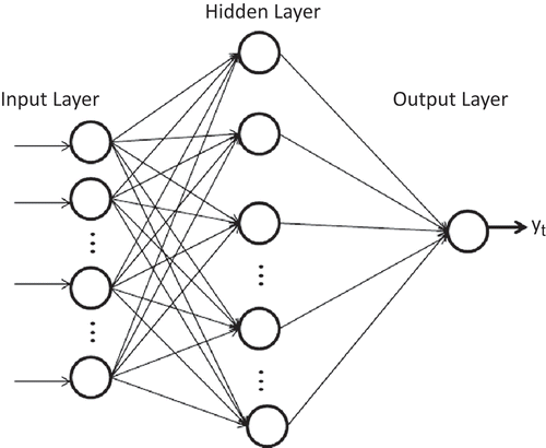
ANNs are flexible computational models that have been extensively studied and used for time series forecasting in many areas of science and engineering since the early 1990s. An ANN is a mathematical model which has a highly connected structure similar to brain cells. The model has the capability of performing complex mapping between inputs and outputs that would enable the network to approximate nonlinear functions. A single hidden layer feed-forward network is the most widely used form of the model for time series modelling and forecasting (Zhang et al. 1998). The model usually consists of three layers: the first layer is the input layer where the data are introduced to the network, the second layer is the hidden layer where data are processed and the last layer is the output layer where the results corresponding to the given inputs are produced. Fig. 1 illustrates the architecture of the proposed ANN for streamflow forecasting. The relationship between the output (y_t ) and the input (y_{t −1}, y_{t −2}, …, y_t−p ) is given by:

(5)

Fig. 1 Architecture of the three-layer feed-forward ANN.

where b_j (j = 0, 1, 2, …, q) and w_ij (i = 0, 1, 2, …, p; j = 0, 1, 2, …, q) are the weights; p is the number of input nodes; q is the number of hidden nodes; f(·) is the transfer function (Coulibaly and Evora 2007); w _0j is a vector of weights from the hidden to output nodes; and w_ij are weights from the input to hidden nodes. Note that equation (5)(5) indicates that a linear transfer function is used in the output node as desired for forecasting problems. The connection weights w_ij of the network are learned through a process called training. The transfer function can appear in several forms, and the most widely used transfer functions are:

Sigmoid function:

(6a)

Linear:

(6b)

Hyperbolic tangent:

(6c)

Generally, ANNs may have different transfer functions for different nodes in the same or different layers. The majority of research uses sigmoid and hyperbolic tangent function transfer functions for hidden nodes and there is no consensus on which transfer function should be used for output nodes (Zhang et al. 1998).

ANN training is an unconstrained nonlinear minimization problem in which the weights of a network are iteratively modified to minimize the overall mean or sum squared error between the desired and actual output values. There is currently no algorithm available to guarantee the global optimal solution for a general nonlinear optimization problem. The most popular neural network training method used is the back-propagation (BP) algorithm which is essentially a steepest gradient descent method introduced by Rumelhart et al. (1986). This algorithm suffers the problems of slow convergence, inefficiency and lack of robustness (Zhang et al. 1998). Furthermore, it can be very sensitive to the choice of the learning rate. It is difficult to choose a proper learning rate, because a low learning rate may result in long training times, and a high learning rate may cause system instability (Maier and Dandy 2000).

To overcome the weakness of the BP algorithm, many researchers have investigated the use of genetic algorithms, simulated annealing, shuffled complex evolution and the Levenberg-Marquardt (LM) algorithm. Among these algorithms, LM is one of the most popular and more efficient nonlinear optimization methods. It is a Hessian-based algorithm for nonlinear least-squares optimization that is used in most optimization packages. The algorithm takes large steps down the gradient where the gradient is small, such as near local minima, and takes small steps when the gradient is large. Its faster convergence, robustness, and the ability to find good local minima make it attractive in ANN training. This optimization technique is more powerful than the conventional gradient descent technique. In recent years, ANNs using the LM algorithm have been shown to give useful results in many fields of hydrology and water resources research (Cigizoglu and Kisi 2005, Affandi and Watanabe 2007, Kisi 2008, 2010, Nourani et al. 2009).

Support vector machine (SVM) model

A SVM is a novel type of learning machine and is fast gaining popularity due to its many attractive features and promising empirical performance (Vapnik 1995). The basic idea of a SVM for regression is to introduce a kernel function, map the input data into a high-dimensional feature space by a nonlinear mapping and then perform linear regression in the feature space. As an illustration, with a given training set of n data points with input data x_i ∈ R^p (p is the total number of data patterns) and output y_i ∈ R, the regression function of SVM is formulated as follows:

(7)

where φ(x) represents the high-dimensional feature space, which is nonlinearly mapped from the input space x. Following the regularization theory, parameters w and b are estimated by minimizing the cost function:

(8)

subject to the constraints:

(9a)

(9b)

(9c)

The first term is the weight vector norm; C is referred to as the regularized constant determining the trade-off between the empirical error and the regularized term; and ε is called the tube size of the SVM, and is equivalent to the approximation accuracy placed on the training data points. The slack variables ξ and ξ* are introduced here. By introducing Lagrange multipliers and exploiting the optimality constraints, the decision function given by equation (5)(5) has the following explicit form:

(10)

In equation (10)(10), a_i and a_i * are assigned as Lagrange multipliers. They satisfy the equalities a_i  × a_i * = 0, a_i ≥ 0 and a_i * ≥ 0 where i = 1, 2, …, n, and these are obtained by maximizing the dual function which has the following form:

(11)

subject to the constraints:

(12a)

(12b)

(12c)

for i = 1, 2, …, n.

The kernel function, K( x _i , x ) can be expressed as the inner product:

(13)

Typical examples of the kernel function are as follows:

Linear:

(14a)

Multilayer perception kernel:

(14b)

Polynomial:

(14c)

Radial basis function (RBF):

(14d)

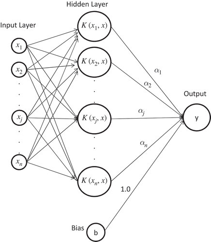
Here γ, r and d are the kernel parameters. The architecture of a SVM is shown in Fig. 2.

Fig. 2 Architecture of SVM.

The least-squares vector machine (LSSVM) model

The LSSVM, as a modification of a SVM, was introduced by Suykens (2000). The LSSVM provides a computational advantage over the standard SVM by converting a quadratic optimization problem into a system of linear equations. This new version of SVM simplifies the problem and converges to a solution quickly. The LSSVM predictor is trained using a set of time series historic values as inputs and a single output as the target value. The LSSVM has been developed to find the optimally non-linear regression function:

(15)

When the LSSVM is used for function estimation, the optimization problem is formulated by minimizing the regular function (Suykens et al. 2002) as:

(16)

subject to the equality constraints:

(17)

To solve this optimization problem, the Lagrange function is constructed as:

(18)

where α _i is a Lagrange multiplier. The solution of equation (18)(18) can be obtained by partially differentiating with respect to w, b, e_i and α _i accordingly:

(19a)

(19b)

(19c)

(19d)

After elimination of e_i and w, the solution is given by the following set of linear equations:

(20)

where y = [y ₁, …, y_n ], 1 = [1; …;1], and α = [α₁, …, α _n ]. This finally leads to the following LSSVM model for function estimation:

(21)

where α _i and b are the solutions to the linear system. For the LSSVM, there are many kernel functions, such as linear, polynomial, radial basis function, sigmoid, etc.

Comparing equation (8)(8) with equation (16)(16), one can see that the LSSVM is a reformulation of the principles of a SVM, which involves equality instead of inequality constraints. Furthermore, the LSSVM uses the least-squares loss function instead of the ε-insensitive loss function. The sparseness contrast between the SVM and the LSSVM is illustrated in Fig. 3 by a linear regression. The left figure presents the SVM with an ε-tube and some slack variables ξ _k * which correspond to two support vectors, while in the LSSVM the ε-tube and the slack variables ξ _k * are replaced by error variables e_k ∈ {e ₁, e ₂, …, e_n }, which give the distances from each point to the regression function.

Fig. 3 Sparseness contrast between SVM and LSSVM for a linear regression.

The SVM is formulated by solving a convex optimization problem, more specifically a quadratic programming problem. This is obtained by employing an inequality constrained optimization problem and exploiting the Mercer condition in order to relate the nonlinear feature space mapping to the chosen kernel function.

The LSSVM is a new technique for regression, and provides a computational advantage over standard SVM by converting a quadratic optimization problem into a system of linear equations (Suykens 2000). The method uses equality constraints instead of inequality constraints and adopts the least-squares linear system as its loss function, which is computationally attractive. The LSSVM also has good convergence and high precision.

STUDY AREA

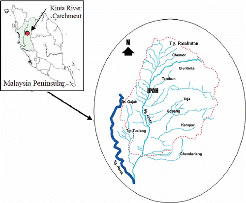
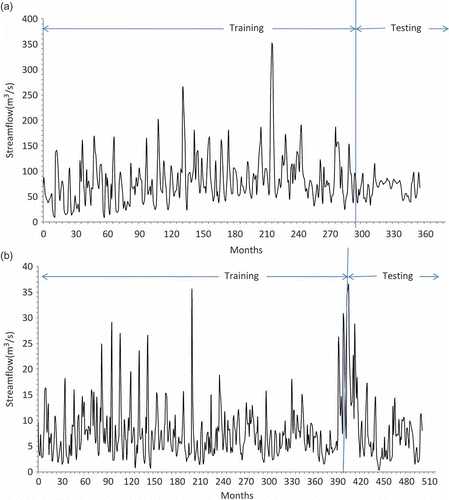
In this study, the monthly streamflow data of Tg Tualang and Tg Rambutan stations on the Kinta River in Perak, Peninsular Malaysia, are used. The Kinta River catchment covers an area of 2500 km². The locations of Tg Tualang and Tg Rambutan stations are shown in Fig. 4. The first set of data comprises the monthly streamflow data of Tg Tualang station from October 1976 to July 2006. In the application, the first 24 years of flow data (287 months, 80% of the whole data set) were used for training the network to obtain the model parameters. Another data set consisting of 72 monthly records (20% of the whole data set) was used for testing. Figure 5 shows the monthly flow of Tg Tualang from October 1976 to July 2006.

Fig. 4 Location map of the study area.

Fig. 5 Time series of monthly streamflow of (a) Tg Tualang and (b) Tg Rambutan stations.

The second data set is the monthly streamflow of Tg Rambutan from January 1961 to December 2002. In the application, the first 32 years of flow data (404 months, 80% of the whole data set) are used for training the network to obtain the model parameters. Another data set consisting of 100 monthly records (20% of the whole data set) are used for testing. Figure 5 shows the monthly flow of Tg Rambutan from January 1961 to December 2002.

The data sets comprising the monthly streamflow statistics are presented in Table 1 for Tg Tualang and Tg Rambutan stations. The observed monthly streamflow data show a close, similarly-skewed distribution for Tg Tualang (2.05) and Tg Rambutan (2.25). However, the range of the streamflow data of Tg Tualang (9.41–351.08 m³/s) is much higher than for Tg Rambutan station (0.36–36.48 m³/s).

Table 1  The statistics for data sets

Station	Data set	Min. (m^3/s)	Standard deviation (m^3/s)	Skewness (m^3/s)	y min (m^3/s)	y max (m^3/s)
Tg Tualang	Training	82.21	48.27	1.85	9.41	351.08
	Testing	69.11	20.22	0.90	33.55	152.93
	Entire	79.54	44.37	2.05	9.41	351.08
Tg Rambutan	Training	7.43	4.88	2.09	0.73	35.33
	Testing	8.39	7.12	2.12	0.36	36.48
	Entire	7.62	5.40	2.25	0.36	36.48

Prior to training the data set, the collected data are normalized so that the transformed values lie between 0 and 1 using the following formula (Swain and Umamahesh 2004):

(22)

where x_t is the normalized value, y_t is the actual value and y _max is the maximum value of the observed data.

Measures of accuracy

The performance of the models in forecasting monthly streamflow during training and testing are evaluated by using the mean absolute error (MAE), the root mean squared error (MSE), the correlation coefficient (R) and the Nash-Sutcliffe coefficient of efficiency (CE), which are widely used for evaluating the results of time series forecasting (Dawson et al. 2007). The MAE, RMSE, R and CE are defined as follows:

(23a)

(23b)

(23c)

(23d)

where y_t° is the observed and y_t ^f is the forecast value at time t, and n is the number of data points. The MAE and RMSE provide different types of information about the predictive capabilities of the model. The MAE and RMSE evaluate how closely the predictions match the observations. The criteria to judge the best model are the relatively small MAE and RMSE found in the training and testing of the data. The correlation coefficient (R) measures how well the predicted flows correlate with the observed flows and shows the degree to which the two variables are linearly related. The coefficient of efficiency (CE) is used to see how well the model performs relative to the mean of the observed time series. Thus a CE value of 0 would imply the model is no better than simply forecasting the mean; R and CE values close to unity indicate a satisfactory result, while a low value or one that is close to zero implies an inadequate result.

MODELLING STRUCTURES

One of the most important steps in developing a satisfactory forecasting model, such as ANN, SVM and LSSVM models, is the selection of the input variables. Appropriate input variables will allow the network to successfully map the desired output and avoid loss of important information. There are no fixed rules in the selection of input variables for developing these models even though a general framework can be followed based on previous successful applications in water resource problems (Bowden et al. 2005, Affandi and Watanabe 2007, Firat 2008, Wang et al. 2009). In this study, eight model structures were developed to investigate the model performance of the input variables. The model structures were obtained by setting the input variables equal to the number of lagged variables from the monthly streamflow of previous periods, y_{t −1}, y_{t −2}, … , y_{t −p} , where p is set to 1, 2, … , 6 months. The other model structures are determined by using stepwise regression analysis (M7) and PACF (M8). The model structure can be mathematically expressed as:

(24)

The various combinations of model structures of the forecasting models considered in the present study are given in Table 2.

Table 2  The model structures for forecasting streamflow of Kinta River

Model	Model input
	Tg Tualang	Tg Rambutan
M1	yt –1	yt –1
M2	yt –1 and yt –2	yt –1 and yt –2
M3	and yt –3	and yt –3
M4	and yt –4	and yt –4
M5	and yt –5	and yt –5
M6	and yt –6	and yt –6
M7	and yt –12	and yt –12
M8	and yt –11	and yt –11

RESULTS AND DISCUSSION

Fitting an ARIMA model to the data

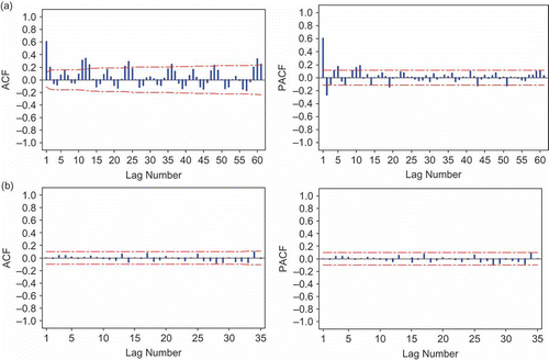
The sample autocorrelation function (ACF) and sample partial autocorrelation function (PACF) for Tg Tualang station on the Kinta River are plotted in Fig. 6(a). The ACF has significance values at lag 1, 2 and multiples of 12. The PACF is damping out in sine waves with significant spikes at lag 1, 2 and 12. This may imply the presence of seasonal and non-seasonal AR and MA terms. The ACF shows that the series is non-stationary, and was differenced by a lag of 12. Five models were initially selected. The best model from the different candidates was identified by using the minimum AIC and the Ljung-Box test, as shown in Table 3. For a good forecasting model, the residuals after fitting the model should be white noise. The Ljung-Box statistics are employed to check the independence of the residuals and to test the adequacy of the model. The first 48 ACF residuals from the models extracted for the calculation of the Q(r) statistics are shown in Table 3. Since the p values are greater than 0.05, the residuals from the models are not significantly different from zero. The Ljung-Box test suggests that there is no autocorrelation left in the residuals, which indicates that the residuals from the selected models are white noise. Therefore, final selected model was the ARIMA (1,0,0)×(2,1,2)₁₂ (Table 3). The residual plots in the ACF and PACF of the residuals are demonstrated in Fig. 6(b). The ACF and PACF of the residuals lie within confidence limits and the residuals did not have a significant correlation, which clearly supports the fact that the residuals from the best model are white noise.

Table 3  Comparison of AIC and Ljung-Box statistics for selected ARIMA models (the best performance indicated by )

Tg Tualang				Tg Rambutan
ARIMA model	AIC	Q(r)	p values	ARIMA model	AIC	Q(r)	p values
(1,0,2)×(1,1,2)12	2825.844	42.4	0.410	(10,1,0)×(0,0,1)12	2270.38	51.2	0.348
(1,0,0)×(2,1,2)12	2812.407	50.3	0.288	(10,1,0)×(1,0,1)12	2272.29	51.3	0.345
(1,0,0)×(1,1,2)12	2824.180	48.3	0.267	(10,1,0)×(1,0,0)12	2270.80	52.0	0.320
(1,0,0)×(0,1,1)12	2824.543	49.1	0.311	(10,1,1)×(1,0,0)12	2272.29	51.3	0.345
(1,0,0)×(1,1,1)12	2822.697	48.7	0.177	(10,1,1)×(0,0,1)12	2272.24	51.2	0.348

Fig. 6 (a) ACF and PACF and (b) ACF and PACF residual of streamflow series at Tg Tualang station.

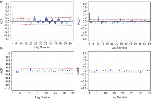
For Tg Rambutan station, the plots of the ACF and PACF are shown in Fig. 7(a). The ACF curves for monthly streamflow data are decayed with a mixture of sine wave patterns and exponential curves with significant spikes near lags 1, 2, 12, 24, 36, 48 and 60. In the PACF, there were significant spikes present near lag 1, 2, 6, 7, 8, 10, 12, 24 and 36. The ACF shows that the series is non-stationary, and was differenced by a lag of 1. Five models were initially selected based on the AIC and Ljung-Box statistic. The identification of the best model for streamflow series based on minimum AIC and Ljung-Box statistics is shown in Table 3, which, based on the AIC, is shown to be the ARIMA (10,1,0)×(0,0,1)₁₂ model. As a second test, the ACF and PACF of the residuals are obtained, as shown in Fig. 7(b). Inspection of the residuals of the ACF and PACF confirmed that the best model is adequate.

Fig. 7 (a) ACF and PACF and (b) ACF and PACF residual of streamflow series at Tg Rambutan station.

Fitting an ANN to the data

The ANN model used in this study is the standard three-layer feed-forward network. Since one-step-ahead forecasting is considered, only one output node is employed. The sigmoid transfer function from the input layer to the hidden layer and the linear function from the hidden layer to the output layer are used for forecasting streamflow time series. The input and target data would be normalized within the range zero to one because a sigmoid function was employed as the transfer function. The application of the linear function at the output layer makes it possible for the network to take any value. However, if the output layers use sigmoid or hyperbolic tangent functions, the outputs are restricted to a small range of values. For forecasting problems, many researchers use a linear function in the output layer, including Dolling and Varas (2003), Coulibaly and Evora (2007), Wang et al. (2009) and Kisi (2009, 2010).

The hidden layer plays an important role in many successful applications of ANNs. It has been proven that only one hidden layer is sufficient for an ANN to approximate any complex nonlinear function with any desired accuracy. In the case of the popular one hidden layer networks, several practical numbers of neurons in the hidden layer were identified for better forecasting accuracy. These include using “2I+1” (Lippmann 1987), “I/2” (Kang 1991), “2I” (Wong 1991) and “I” (Tang and Fishwick 1993), where I is the number of inputs. However, as far as the number of hidden neurons is concerned, there is currently no theory to determine how many nodes in the hidden layer are optimal. The optimal complexity of the ANN model, that is the number of input and hidden neurons, will be determined as it is usually done by a trial-and-error approach. In the present study, the eight models (M1–M8) having various input structures were trained and tested using ANN models. For each input layer dimension, the number of hidden nodes was progressively increased from 1 to 10.

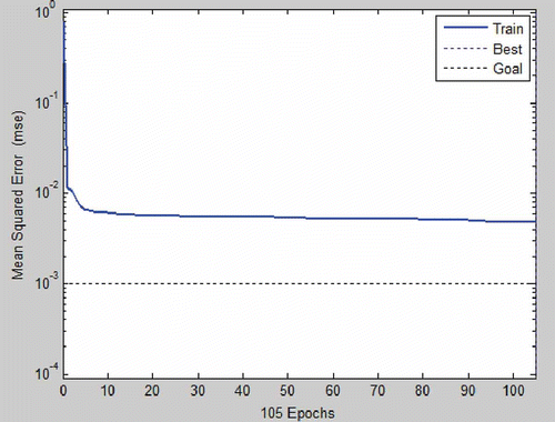
In this study we use the Levenberg-Marquardt (LM) algorithm provided by the MATLAB neural network toolbox for ANN training. Figure 8 indicates that the ANN model for streamflow forecasting data reaches the present training goal of 0.004 86 after 100 epochs with a mean square error (MSE) falling in the range of 0.01 to 0.001. The ANN network training was stopped after 100 epochs as the variation in error was too small after this epoch. In this study, the training determination condition was set to a total of 100 epochs or to an MSE of 0.001.

Fig. 8 The training error graph for the ANN model.

Table 4 shows the performance results for different ANN models with different numbers of hidden neurons (between 1 and 10). The performance of the ANNs varies in accordance with the number of neurons in the hidden layer. For the training phase for Tg Tualang station, the M8 model with five hidden neurons resulted in the best MSE, MAE, R and CE. In the testing phase, M6 (four hidden neurons) obtained the best MAE (11.855), while M7 (two hidden neurons) obtained the best RMSE, R and CE statistics (17.058, 0.610 and 0.278, respectively). For the training phase for Tg Rambutan station, the M7 model with five hidden neurons obtained the best RMSE, MAE, R and CE statistics of 3.351, 2.308, 0.727 and 0.529, respectively. In the testing phase, M1 (three hidden neurons) obtained the best R value (0.762), and M2 (eight hidden neurons) the best MAE (3.153), while M7 (five hidden neurons) obtained the best RMSE and CE statistics (4.832 and 0.535, respectively).

Table 4  Forecasting performance indices of ANN for Tg Tualang and Tg Rambutan stations (the best performance indicated by )

Station	Model structure		Training				Testing
			RMSE	MAE	R	CE	RMSE	MAE	R	CE
Tg Tualang	M1	1×3×1	37.357	28.329	0.633	0.401	18.171	13.101	0.462	0.181
	M2	2×2×1	36.258	27.260	0.661	0.438	18.102	12.849	0.510	0.187
	M3	3×9×1	32.777	24.358	0.736	0.542	17.541	13.873	0.584	0.237
	M4	4×6×1	33.546	25.005	0.721	0.520	18.022	12.252	0.551	0.195
	M5	5×5×1	31.755	23.720	0.755	0.571	17.258	12.110	0.564	0.261
	M6	6×4×1	35.378	26.352	0.684	0.467	17.192	11.855	0.587	0.267
	M7	6×2×1	33.384	24.638	0.725	0.526	17.058	12.541	0.610	0.278
	M8	6×5×1	29.766	21.539	0.788	0.621	17.255	12.256	0.590	0.262
Tg Rambutan	M1	1×3×1	4.230	2.811	0.497	0.246	5.075	3.250	0.762	0.487
	M2	2×8×1	4.256	2.783	0.489	0.238	4.985	3.153	0.730	0.505
	M3	3×5×1	4.017	2.639	0.568	0.322	5.032	3.262	0.711	0.495
	M4	4×5×1	4.082	2.688	0.550	0.301	5.569	3.435	0.690	0.382
	M5	5×5×1	3.983	2.632	0.580	0.336	5.499	3.387	0.706	0.397
	M6	6×2×1	4.113	2.740	0.541	0.293	5.196	3.286	0.688	0.462
	M7	4×5×1	3.351	2.308	0.727	0.529	4.832	3.287	0.734	0.535
	M8	6×1×1	3.996	2.630	0.573	0.332	4.840	3.347	0.732	0.508

Based on the performance indices in the testing phase, the ANN(6,2,1) and ANN(4,5,1) models using M7 were selected for Tg Tualang and Tg Rambutan, respectively.

Fitting a SVM to the data

In the training and testing of the SSVM model, the same input structures of the data set (M1–M8) are used. This paper focuses on the use of the RBF kernel for its effective performance and advantages in solving the time series forecasting problem, as has been proven in past research. Previous works on the use of SVM in hydrological modelling and forecasting have shown favourable performance from RBFs (Dibike et al. 2001, Khalil et al. 2005). The advantage of the RBF kernel is that it nonlinearly maps the training data into a possibly infinite dimensional space. This can effectively handle situations when the predictors and predicted are nonlinear, and it is more computationally simple than the polynomial kernel.

The optimal parameter search of the SVM plays an important role in the building of a streamflow forecasting model with high forecasting accuracy and stability. To make an efficient SVM model, three parameters C, ε and γ must be carefully predetermined. The model selection and parameter search play a crucial role in the performance of the SVM. It is well known that SVM generalization performance (estimation accuracy) depends on finding good values of these parameters. For each problem, the generalized accuracy is estimated using different parameters C, ε and γ. The range of the search was set to [1,10] at increments of 1.0 for C, and [0.1,0.5] at increments of 0.1 for ε, with γ fixed as 0.5. Therefore, for each problem, trials of 10 × 5 = 50 combinations were carried out. One of the most popular techniques for evaluating a set of parameter values is the use of cross-validation. For each parameter pair (C, ε) in the search space, 10-fold cross-validation is conducted on the training set, and the optimal values of (C, ε) are selected. Cross-validation is repeated ten times to increase the reliability of the results. For the final prediction used in the competition, we used all of the available data to train the models with the parameters producing minimum validation errors. The parameter values that yield the minimum generalization error are chosen.

Table 5 shows the performance results obtained in the training and testing periods of the SVM approach for Tg Tualang and Tg Rambutan stations. It may be seen from Table 5 that for Tg Tualang, in the training phase, the SVM model has the smallest RMSE and MAE, and the highest R for model M8, while the highest CE was obtained with model M5. However, in the testing phase, M5 obtained the best RMSE, MAE and CE, whereas the best R was obtained by M8. For Tg Rambutan station, the training phase results show that M7 has the best values of RMSE, MAE, R and CE. In the testing phase, the best RMSE, R and CE were obtained for M8, whereas the best MAE was for M7.

Table 5  Forecasting performance indices of SVM for Tg Tualang and Tg Rambutan stations (the best performance indicated by )

Station	Model	Training				Testing
		RMSE	MAE	R	CE	RMSE	MAE	R	CE
Tg Tualang	M1	49.657	42.812	0.608	−0.050	40.892	38.186	0.457	−3.146
	M2	37.578	26.881	0.645	0.399	17.277	12.221	0.524	0.260
	M3	37.082	26.539	0.656	0.415	17.196	12.080	0.531	0.267
	M4	52.391	46.218	0.642	−0.169	45.948	43.747	0.470	−4.235
	M5	35.862	25.167	0.681	0.452	16.715	11.393	0.565	0.307
	M6	36.557	27.858	0.665	0.262	19.426	15.060	0.563	0.064
	M7	35.427	25.206	0.690	0.307	16.972	12.072	0.579	0.286
	M8	34.548	24.653	0.710	0.341	16.785	12.046	0.597	0.301
Tg Rambutan	M1	5.778	4.961	0.437	−0.407	6.325	5.265	0.726	0.203
	M2	4.291	2.874	0.486	0.225	5.911	3.717	0.658	0.303
	M3	4.262	2.840	0.496	0.237	5.785	3.632	0.671	0.333
	M4	4.259	2.825	0.496	0.239	5.860	3.667	0.653	0.315
	M5	4.251	2.826	0.503	0.244	5.903	3.713	0.640	0.305
	M6	4.207	2.820	0.520	0.260	5.386	3.487	0.707	0.422
	M7	3.981	2.503	0.874	0.334	5.210	3.175	0.736	0.469
	M8	3.989	2.542	0.587	0.332	5.017	3.220	0.738	0.508

Fitting the LSSVM to the data

There is no theory that can be used to guide the selection of the optimal number of input nodes and parameters of the LSSVM model. In order to obtain the optimal model parameters of the LSSVM, a grid search algorithm and cross-validation method were employed. A grid search of (γ,σ²) with γ in the range 10 to 1000 and σ² in the range 0.01 to 1.0 was considered. For each hyper parameter pair (γ,σ²) in the search space, 10-fold cross-validation on the training set was performed to predict the prediction error. The best fit model structure for each model is determined according to the criteria of the performance evaluation. Previous work on the use of LSSVM in time series modelling and forecasting have demonstrated favourable performance of RBFs (Liu and Wang 2008, Gencoglu and Ulyar 2009). Therefore, a RBF was used as the kernel function for streamflow forecasting in this study.

Table 6 shows the performance results obtained in the training and testing periods of the LSSVM approach. For Tg Tualang station, the best values of RMSE, MAE, R and CE for the training and testing phases were obtained using model M7; however, in the testing phase alone, the best RMSE, R and CE values were obtained using M7, while the best MAE was obtained using model M5. For Tg Rambutan station, the model input M7 gave the best performance for the LSSVM model for the training phase. In the testing phase, M4 had the smallest RMSE and MAE and the highest CE, whereas the highest value of R was obtained using M1.

Table 6  Forecasting performance indices of LSSVM for Tg Tualang and Tg Rambutan stations (the best performance indicated by )

Station	Model	Training				Testing
		RMSE	MAE	R	CE	RMSE	MAE	R	CE
Tg Tualang	M1	38.103	28.601	0.614	0.377	18.172	12.881	0.476	0.181
	M2	37.991	27.928	0.650	0.383	17.566	13.458	0.562	0.235
	M3	37.892	28.025	0.657	0.387	17.907	12.539	0.593	0.205
	M4	38.068	28.003	0.644	0.383	17.991	12.585	0.553	0.197
	M5	36.908	26.776	0.668	0.420	17.157	11.965	0.571	0.270
	M6	36.044	26.210	0.681	0.447	17.356	12.339	0.571	0.253
	M7	30.225	21.664	0.889	0.609	16.496	12.259	0.652	0.325
	M8	36.013	26.337	0.688	0.448	17.455	12.733	0.581	0.245
Tg Rambutan	M1	4.248	2.838	0.491	0.239	4.995	3.178	0.761	0.503
	M2	4.177	2.761	0.517	0.266	5.229	3.295	0.721	0.455
	M3	4.020	2.682	0.568	0.321	5.079	3.161	0.698	0.486
	M4	3.932	2.580	0.594	0.351	4.801	3.137	0.737	0.541
	M5	3.946	2.606	0.592	0.348	5.714	3.523	0.594	0.349
	M6	3.968	2.664	0.589	0.342	5.675	3.591	0.602	0.358
	M7	3.723	2.525	0.649	0.417	5.370	3.505	0.659	0.425
	M8	3.850	2.546	0.615	0.378	5.135	3.312	0.719	0.474

Based on these criteria, model M7 was selected as the best-fit streamflow forecasting model for Tg Tualang station, and model M4 was selected for Tg Rambutan station.

Comparison of the forecasting models

We investigated a soft computing LSSVM model for streamflow forecasting and compared the results with ARIMA, ANN and SVM models. For further analysis, the best performances were compared for the ARIMA, ANN, SVM and LSSVM models in terms of the MAE, MSE and R in the testing phase. Table 7 presents the results for the Tg Tualang and Tg Rambutan study stations, in terms of the various performance statistics.

Table 7  The performance results of ARIMA, ANN, SVM and LSSVM approaches in the testing period (the best performance indicated by )

Model	Tg Tualang				Tg Rambutan
	RMSE	MAE	R	CE	RMSE	MAE	R	CE
ARIMA	21.783	17.486	0.525	−0.130	4.909	3.286	0.754	0.520
ANN	17.058	12.541	0.610	0.278	4.832	3.287	0.734	0.535
SVM	16.715	11.393	0.565	0.307	5.017	3.220	0.738	0.508
LSSVM	16.496	12.259	0.652	0.325	4.801	3.137	0.737	0.541

In Table 7, it is shown that, for Tg Tualang station, various AI methods, i.e. ANN, SVM and LSSVM, present a good performance in the testing phase, and they outperform ARIMA in terms of all the standard statistical measures. The LSSVM model obtained the best RMSE, R and CE, while the SVM model obtained the best MAE statistics. However for Tg Rambutan, the best performances of all AI methods developed herein differ in terms of the different statistical measures compared with the ARIMA model. The LSSVM model has the smallest RMSE, MAE and CE, while the ARIMA has the largest R value (Table 7). Although the ARIMA model produced estimates with higher R for Tg Rambutan station, this increase in R was not associated with an improvement in the magnitude of the other error measures (RMSE, MAE and CE). Although R and R ² statistics have been widely used for model evaluation (Lin et al. 2006, Kisi 2008, Hung et al. 2009, Adamowski and Sun 2010), they are oversensitive to outliers and insensitive to additive and proportional differences between the observed and modelled data sets (Dawson et al. 2007, Wang et al. 2009).

Generally, in the testing data set it can be observed that the LSSVM model outperforms all other models for both Tg Tualang and Tg Rambutan stations. Thus, the results indicate that the LSSVM is able to obtain the best results in terms of different evaluation measures in the testing phase for both stations.

The observed and estimated flows from the ARIMA, ANN, SVM and LSSVM are shown in Figs 9 and 10, for Tg Tualang and Tg Rambutan, respectively, in the form of a hydrograph and scatter plot. These graphs show that the AI predictions (ANN, SVM and LSSVM) and ARIMA model are closer to the corresponding observed streamflow values for Tg Rambutan station, and the AI predictions are closer to the corresponding observed values than the ARIMA model for Tg Tualang station. The observed streamflows in the testing period for Tg Tualang station contain some extreme values (outliers) compared with Tg Rambutan station, and the ARIMA model tends to fail to capture the pattern of these extreme values. This condition finally implies that the performance of the ARIMA models is worse compared to the other methods. The better performance of the AI models indicates that the AI models are able to capture the nonlinear and highly complex behaviour of the streamflow process, while the ARIMA model is only a class of linear univariate models and thus it can only capture linear features of time series data.

Fig. 9 Predicted and observed streamflow in the testing period by ARIMA, ANN, SVM and LSSVM: Tg Tualang station.

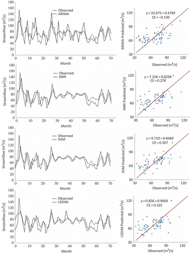
Fig. 10 Predicted and observed streamflow in the testing period by ARIMA, ANN, SVM and LSSVM: Tg Rambutan station.

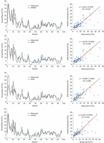
As seen from the fit line equation (y = a + bx) and the coefficient of efficiency (CE) in the scatter plots, the LSSVM model is slightly superior to the other models for both Tg Tualang and Tg Rambutan stations.

The results obtained in this study indicate that the LSSVM model is capable of providing a good modelling method and may provide an alternative to the SVM, ANN and ARIMA models for forecasting monthly streamflow.

CONCLUSION

Monthly streamflow forecasting is vital in hydrological practices. There are plenty of methods that could be used to forecast streamflow. In this paper, we introduce a LSSVM to forecast the streamflow time series. The LSSVM is the reformulation of the principles of SVM. The standard SVM is solved by quadratic programming methods; however, these methods are often time-consuming and difficult to implement adaptively, and suffer from the problem of large memory requirement. The LSSVM is a modified version of SVM, encompasses similar advantages to the SVM, but has additional advantages because it solves the regression problem using a set of linear equations instead of quadratic programming. Therefore, the LSSVM is much easier to use and has a shorter computing time compared to SVM.

To illustrate the capability of the LSSVM model, Tg Tualang and Tg Rambutan stations on the Kinta River, located in Perak, Peninsular Malaysia, were chosen as case studies. One of the most important steps in developing a satisfactory forecasting model such as an ANN, SVM and LSSVM is the selection of the input variables. Models with various input variables were trained and tested for both stations to investigate the accuracy of the LSSVM compared with the ANN, SVM and ARIMA models. The performance of these models was compared and evaluated based on their performance on the training and the testing data sets. By comparing the results of the testing data set, it can be seen that, for Tg Tualang station, the input variables equal the number of lagged variables from monthly streamflow of the previous period of data; M7, M5 and M7 had the best performance for the ANN, SVM and LSSVM models, respectively. However, for Tg Rambutan station, the best performance was shown by M7 for the ANN, M8 for the SVM and M4 for the LSSVM model.

The best fitting ARIMA, ANN, SVM and LSSVM models for both Tg Tualang and Tg Rambutan stations in the testing phase were compared. The LSSVM was found to be better than other models for both stations, in monthly streamflow forecasting. The overall comparison suggests that the LSSVM model outperforms, or performs as well as, the other models and may therefore provide an alternative to ANN, SVM and ARIMA models for forecasting monthly streamflow in situations that do not require the modelling of the internal structure of the watershed.

Acknowledgements

This paper is supported by a Research University Grant Scheme of the Universiti Teknologi Malaysia under vote number 02J26. Also the authors gratefully acknowledge the critical comments and corrections of the anonymous reviews; their comments significantly improved the original manuscript.

REFERENCES

- Adamowski , J. and Sun , K. 2010 . Development of a coupled wavelet transform and neural network method for flow forecasting of non-perennial rivers in semi-arid watersheds . Journal of Hydrology , 390 ( 1–2 ) : 85 – 91 .
- Affandi , A.K. and Watanabe , K. 2007 . Daily groundwater level fluctuation forecasting using soft computing technique . Nature and Science , 5 ( 2 ) : 1 – 10 .
- Akaike , H. 1974 . A new look at the statistical model identification . IEEE Transactions on Automatic Control , 19 : 716 – 723 .
- Afshin , M. , Sadeghian , A. and Raahemifar , K. 2007 . On efficient tuning of LS-SVM hyper-parameters in short-term load forecasting: a comparative study . Proceedings of the 2007 IEEE Power Engineering Society General Meeting (IEEE-PES) . 2007 .
- Asefa , T. 2006 . Multi-time scale stream flow prediction: the support vector machines approach . Journal of Hydrology , 318 ( 1–4 ) : 7 – 16 .
- Birkinshaw , S.J. , Parkin , G. and Rao , Z. 2008 . A hybrid neural networks and numerical models approach for predicting groundwater abstraction impacts . Journal of Hydroinformatics , 10 ( 2 ) : 127 – 137 .
- Bowden , G.J. , Dandy , G.C. and Maier , H.R. 2005 . Input determination for neural network models in water resources applications. Part 1 – Background and methodology . Journal of Hydrology , 301 ( 1–4 ) : 75 – 92 .
- Box , G.E.P. and Jenkins , G. 1970 . Time series analysis. forecasting and control , San Francisco , CA : Holden-Day .
- Brockwell , P.J. and Davis , R.A. 2002 . Introduction to time series and forecasting , Berlin : Springer .
- Cigizoglu , H.K. and Kisi , O. 2005 . Flow prediction by three back propagation techniques using k-fold partitioning of neural network training data . Nordic Hydrology , 36 ( 1 ) : 1 – 16 .
- Coulibaly , P. and Evora , N.D. 2007 . Comparison of neural network methods for infilling missing daily weather records . Journal of Hydrology , 341 : 27 – 41 .
- Dibike , Y.B. 2001 . Model induction with support vector machines: introduction and applications . ASCE Journal of Computing in Civil Engineering , 15 ( 3 ) : 208 – 216 .
- Dawson , C.W. , Abrahart , R.J. and See , L.M. 2007 . HydroTest: A web-based toolbox of evaluation metrics for the standardized assessment of hydrological forecasts . Environmental Modelling and Software , 22 : 1034 – 1052 .
- Dolling , O.R. and Varas , E.A. 2003 . Artificial neural networks for streamflow prediction . Journal of Hydraulic Research , 40 ( 5 ) : 547 – 554 .
- Fernandez , C. and Vega , J.A. 2009 . Streamflow drought time series forecasting: a case study in a small watershed in north west Spain . Stochastic Environmental Research and Risk Assessment , 23 : 1063 – 1070 .
- Firat , M. 2008 . Comparison of Artificial Intelligence techniques for river flow forecasting . Hydrology and Earth System Sciences , 12 : 123 – 139 .
- Gencoglu , M.T. and Uyar , M. 2009 . Prediction of flashover voltage of insulators using least square support vector machines . Expert Systems with Applications , 36 : 10789 – 10798 .
- Gestel , T.V. 2001 . Financial time series prediction using least squares support vector machines within the evidence framework . IEEE Transactions on Neural Networks , 12 ( 4 ) : 809 – 821 .
- Hu , T.S. , Lam , K.C. and Ng , S.T. 2001 . River flow time series prediction with range-dependent neural network . Hydrological Sciences Journal , 46 ( 5 ) : 729 – 745 .
- Huang , W. , Bing Xu , B. and Hilton , A. 2004 . Forecasting flow in Apalachicola River using neural networks . Hydrological Processes , 18 : 2545 – 2564 .
- Hung , N.Q. 2009 . An artificial neural network model for rainfall forecasting in bangkok, Thailand . Hydrology and Earth System Sciences , 13 : 1413 – 1425 .
- Jain , A. and Kumar , A.M. 2007 . Hybrid neural network models for hydrologic time series forecasting . Applied Soft Computing , 7 : 585 – 592 .
- Kang , S. 1991 . An investigation of the use of feedforward neural network for forecasting , USA : Thesis (PhD), Kent State University .
- Keskin , M.E. and Taylan , D. 2009 . Artificial models for interbasin flow prediction in southern Turkey . Journal of Hydrologic Engineering , 14 ( 7 ) : 752 – 758 .
- Khalil , A. 2005 . Applicability of statistical learning machine algorithms in groundwater quality modeling . Water Resources Research , 41 : W05010 doi: 10.1029/2004WR003608
- Kisi , O. 2004 . River flow modeling using artificial neural networks . Journal of Hydrologic Engineering , 9 ( 1 ) : 60 – 63 .
- Kisi , O. 2008 . River flow forecasting and estimation using different artificial neural network techniques . Hydrology Research , 39 ( 1 ) : 27 – 40 .
- Kisi , O. 2009 . Neural network and wavelet conjunction model for modeling monthly level fluctuations in Turkey . Hydrological Processes , 23 : 2081 – 2092 .
- Kisi , O. 2010 . Wavelet regression model for short-term streamflow forecasting . Journal of Hydrology , 389 : 344 – 353 .
- Lin , J.Y. , Cheng , C.T. and Chau , K.W. 2006 . Using support vector machines for long-term discharge prediction . Hydrological Sciences Journal , 51 ( 4 ) : 599 – 612 .
- Liong , S.Y. and Sivapragasam , C. 2002 . Flood stage forecasting with support vector machines . JAWRA Journal of the American Water Resources Association , 38 ( 1 ) : 173 – 186 .
- Lippmann , R.P. 1987 . An introduction to computing with neural nets . IEEE ASSP Magazine , 4 ( 2 ) : 4 – 22 .
- Liu , L. and Wang , W. 2008 . Exchange rates forecasting with least squares support vector machines . International Conference on Computer Science and Software Engineering , : 1017 – 1019 .
- Luk , K.C. , Ball , J.E. and Sharma , A. 2000 . A study of optimal model lag and spatial inputs to artificial neural network for rainfall forecasting . Journal of Hydrology , 227 : 56 – 65 .
- Maier , H.R. and Dandy , G.C. 2000 . Neural networks for the production and forecasting of water resource variables: a review and modelling issues and application . Environmental Modelling and Software , 15 : 101 – 124 .
- Modarres , R. 2007 . Streamflow drought time series forecasting . Stochastic Environmental Research and Risk Assessment , 21 : 223 – 233 .
- Muhamad , J.R and Hassan , J.N. 2005 . Khabur River flow using artificial neural networks . Al-Rafidain Engineering , 13 ( 2 ) : 33 – 42 .
- Nourani , V. , Alami , M.T. and Aminfar , M.H. 2009 . A combined neural-wavelet model for prediction of Ligvanchai watershed precipitation . Engineering Applications of Artificial Intelligence , 22 : 466 – 472 .
- Rajurkar , M.P. , Kothyari , U.C. and Chaube , U.C. 2002 . Artificial neural networks for daily rainfall–runoff modelling . Hydrological Sciences Journal , 47 ( 6 ) : 865 – 877 .
- Rumelhart , D.E. , Hinton , G.E. and Williams , R.J. 1986 . Learning representations by back-propagating errors . Nature , 323 : 533 – 536 .
- Shamseldin , A. , Nasr , A.E. and O'Connor , K.M. 2002 . Comparison of different forms of the multi-layer feed-forward neural network method used for river flow forecasting . Hydrology and Earth System Sciences , 6 ( 4 ) : 671 – 684 .
- Shamseldin , A. , O'Connor , K.M. and Nasr , A.E. 2007 . A comparative study of three neural network forecast combination methods for simulated river flows of different rainfall—runoff models . Hydrological Sciences Journal , 52 ( 5 ) : 896 – 916 .
- Sivapragasam , C. and Liong , S.Y. 2005 . Flow categorization model for improving forecasting . Nordic Hydrology , 36 ( 1 ) : 37 – 48 .
- Sun , G. and Guo , W. 2005 . Robust mobile geo-location algorithm based on LSSVM . IEEE Transactions on Vehicular Technology , 54 ( 3 ) : 1037 – 1041 .
- Suykens , J.A.K. 2000 . Least squares support vector machines for classification and nonlinear modelling . Neural Network World , 10 ( 1–2 ) : 29 – 48 . Special Issue on PASE 2000
- Suykens , J.A.K. and Vandewalle , J. 1999 . Least squares support vector machine classifiers . Neural Processes Letters , 9 ( 3 ) : 293 – 300 .
- Suykens , J.A.K. 2002 . Least squares support vector machines , Singapore : World Scientific .
- Swain , P.C. and Umamahesh , N.V. Streamflow forecasting using neuro-fuzzy inference system . International Conference on Advanced Modeling Techniques for Sustainable Management of Water Resources .
- Tang , Z. and Fishwick , P.A. 1993 . Feedforward neural nets as models for time series forecasting . ORSA Journal on Computing , 5 ( 4 ) : 374 – 385 .
- Vapnik , V. 1995 . The nature of statistical learning theory , Berlin : Springer Verlag .
- Vapnik , V. 1999 . An overview of statistical learning theory . IEEE Transactions on Neural Networks , 10 ( 5 ) : 988 – 999 .
- Wang , H. and Hu , D. 2005 . Comparison of SVM and LS-SVM for regression . IEEE International Conference Neural Networks and Brain , : 279 – 283 .
- Wang , W.C. 2009 . A comparison of performance of several artificial intelligence methods for forecasting monthly discharge time series . Journal of Hydrology , 374 : 294 – 306 .
- Wong , F.S. 1991 . Time series forecasting using backpropagation neural networks . Neurocomputing , 2 : 147 – 159 .
- Wu , C.L. and Chau , K.W. 2010 . Data-driven models for monthly streamflow time series prediction . Engineering Applications of Artifical Intelligence , 23 : 1350 – 1367 .
- Xiang , Y. and Jiang , L. 2009 . Water quality prediction using LS-SVM with particle swarm optimization . Second International Workshop on Knowledge Discovery and Data Mining , : 900 – 904 .
- Yu , P.S. , Chen , S.T. and Chang , I.F. 2006 . Support vector regression for real-time flood stage forecasting . Journal of Hydrology , 328 ( 3–4 ) : 704 – 716 .
- Yurekli , K. , Kurunc , A. and Simsek , H. 2004 . Prediction of daily streamflow based on stochastic approaches . Journal of Spatial Hydrology , 4 ( 2 ) : 1 – 12 .
- Zhang , B. and Govindaraju , R.S. 2000 . Prediction of watershed runoff using Bayesian concepts and modular neural networks . Water Resources Research , 36 ( 3 ) : 753 – 762 .
- Zhang , G. , Patuwo , B.E. and Hu , M.Y. 1998 . Forecasting with artificial neural networks: the state of the art . International Journal of Forecasting , 14 : 35 – 62 .
- Zhang , G.P. 2003 . Time series forecasting using a hybrid ARIMA and neural network model . Neurocomputing , 50 : 159 – 175 .