Modelling heteroscedasticty of streamflow times series

Abstract

Time series modelling approaches are useful tools for simulating and forecasting hydrological variables and their change through time. Although linear time series models are common in hydrology, the nonlinear time series model, the Generalized Autoregressive Conditional Heteroscedasticity (GARCH) model, has rarely been used in hydrology and water resources engineering. The GARCH model considers the conditional variance remaining in the residuals of the linear time series models, such as an ARMA or an ARIMA model. In the present study, the advantages of a GARCH model against a linear ARIMA model are investigated using three classes of the GARCH approach, namely Power GARCH, Threshold GARCH and Exponential GARCH models. A daily streamflow time series of the Matapedia River, Quebec, Canada, is selected for this study. It is shown that the ARIMA (13,1,4) model is adequate for modelling streamflow time series of Matapedia River, but the Engle test shows the existence of heteroscedasticity in the residuals of the ARIMA model. Therefore, an ARIMA (13,1,4)-GARCH (3,1) error model is fitted to the data. The residuals of this model are examined for the existence of heteroscedasticity. The Engle test indicates that the GARCH model has considerably reduced the heteroscedasticity of the residuals. However, the Exponential GARCH model seems to completely remove the heteroscedasticity from the residuals. The multi-criteria evaluation for model performance also proves that the Exponential GARCH model is the best model among ARIMA and GARCH models. Therefore, the application of a GARCH model is strongly suggested for hydrological time series modelling as the conditional variance of the residuals of the linear models can be removed and the efficiency of the model will be improved.

Editor D. Koutsoyiannis; Associate editor C. Onof

Citation Modarres, R. and Ouarda, T.B.M.J., 2013. Modelling heteroscedasticty of streamflow times series. Hydrological Sciences Journal, 58 (1), 1–11.

Résumé

Les approches de modélisation des séries temporelles sont des outils utiles pour la simulation et la prévision des variables hydrologiques et de leur évolution à cours du temps. Si les modèles linéaires de séries temporelles sont courants en hydrologie, les modèles non linéaires de séries temporelles, comme le modèle d'hétéroscédasticité conditionnel autorégressif généralisé (GARCH pour l'acronyme anglais), ont rarement été utilisés en hydrologie et en ingénierie des ressources en eau. Le modèle GARCH considère la variance conditionnelle restante des résidus de modèles linéaires de séries temporelles, tels que les modèles ARMA ou ARIMA. Dans la présente étude, nous avons étudié les avantages d'un modèle GARCH par rapport à un modèle linéaire ARIMA en utilisant trois approches de type GARCH, à savoir le modèle GARCH puissance, le modèle GARCH seuil et le modèle GARCH exponentiel. Une série de débits journaliers de la rivière Matapédia, au Québec, Canada, a été choisie pour cette étude. On a montré que le modèle ARIMA (13,1,4) est adéquat pour modéliser la série des débits de la rivière Matapédia, mais le test d'Engle montre l'existence d'une hétéroscédasticité dans ses résidus. Par conséquent, un modèle d'erreur ARIMA (13,1,4)-GARCH (3,1) a été ajusté aux données et on a examiné s'il existait une hétéroscédasticité dans les résidus de ce modèle. Le test d'Engle indique que le modèle GARCH a considérablement réduit l'hétéroscédasticité des résidus, et le modèle GARCH exponentiel semble même la supprimer complètement. L'évaluation multi-critères de la performance du modèle prouve également que le modèle GARCH exponentiel est le meilleur parmi les modèles ARIMA et GARCH. Par conséquent, l'application d'un modèle GARCH est fortement recommandée pour la modélisation des séries temporelles hydrologiques, étant donné que la variance conditionnelle des résidus des modèles linéaires peut être éliminée et que l'efficacité du modèle en sera améliorée.

Key words:

• heteroscedasticity
• Generalized Autoregressive Conditional Heteroscedasticity (GARCH)
• Engle test
• Exponential GARCH
• streamflow time series

Mots clefs:

• hétéroscédasticité
• GARCH
• test d'Engle
• GARCH exponentiel
• série temporelle de débit

1 INTRODUCTION

Time series modelling has been an important topic in hydrology, water resources and climate sciences for decades, as it is a useful tool in hydrological analysis, forecasting and simulation. The linear time series models have been widely applied for different hydrological and climatic variables such as rainfall (Machiwal and Jha 2008), streamflow (Ouarda et al. 1997), floods (Toth et al. 1999), droughts (Modarres 2007) and water quality variables (Kurunc et al. 2005). Time series models in hydrology are often linear models that generally focus on modelling and predicting the mean behaviour, or the first moment of the variable. These models are usually insufficient for capturing the nonlinear properties of the processes governing the temporal variation of hydrological variables.

Recently, there has been a growing interest in applying nonlinear time series models in hydrology. Investigations on nonlinearity and applications of nonlinear models to hydrological variables have received considerable attentions in the recent decades. For example, Rao and Yu (1990) investigated the nonlinear characteristics of annual streamflow and daily rainfall and temperature time series. They reported the existence of nonlinearity in daily meteorological series but nonlinearity was not observed in the annual streamflow time series. Chen and Rao (2003) investigated the nonlinear behaviour of monthly hydrological time series and indicated that all of the stationary segments of standardized monthly temperature and precipitation series are either Gaussian or linear, and some of the standardized monthly streamflows are nonlinear. Wang et al. (2006) indicated that annual streamflow time series are linear, while daily streamflow time series are nonlinear. This nonlinearity behaviour of streamflows weakens as the time scale of the data increases from a day to a year.

Although the linearity in the mean or the first moment of hydrological variables can be captured by linear time series models, the variance or the second-order moment of hydrological variables that may be responsible for nonlinearity is rarely considered in time series modelling. The Generalized AutoRegressive Conditional Heteroscedasticity model (GARCH), originating from econometrics, provides an appropriate framework for focusing on the nonlinearity behaviour of the second-order moment of hydrological variables. This type of model was proposed by Engle (1982) for modelling the conditional variance, or time varying variance, of financial time series and developed by Bollerslev (1986). It represents a nonlinear model which applies the past variance in the explanation of the future variance. This type of model has not received much attention as yet from the hydrological community. A few studies, such as Wang et al. (2005), Wang (2006) and Chen et al. (2008), have applied and discussed the advantage of GARCH-type models in streamflow time series modelling.

The aim of the present paper is to apply GARCH-type models in streamflow time series modelling in order to illustrate the advantages of these nonlinear models over the linear ARIMA model usually applied in hydrological time series modelling. We also introduce and apply three sub-classes of the GARCH model herein.

2 METHODS

2.1 ARIMA model

The linear time series model used in this study is the popular Autoregressive Integrated Moving Average (ARIMA) model, which may be applied for seasonal and nonseasonal time series. The ARIMA model used herein does not include the seasonal parameters and can be written as follows (Hipel and McLeod 1996):

(1)

where Y_t is the observed time series, φ _b (B) is a polynomial of order p, φ _q (B) is a polynomial of order q, ∇ ^d is the nonseasonal differencing operator, B is the backward operator and ε _t is an independent identically distributed (i.i.d) normal error with a zero mean and standard deviation σ. The nonseasonal differencing operator, which is selected just large enough to remove all of nonseasonal nonstationarity, is given by:

(2)

Linear model building has three steps, namely model identification, model estimation and model diagnostic checking. For the sake of brevity, the reader is referred to Hipel and McLeod (1996) for more details.

2.2 GARCH model

2.2.1 General theory

The nonlinear model used in this study includes the GARCH model and its varieties commonly applied in econometrics. This approach considers the volatility or the conditional variance (σ _t ) of a single asset return and tries to model the volatility process of a univariate variable, Y_t . In this case we have:

(3)

where denotes the conditional variance that satisfies the equation:

(4)

The first part of the above model, first introduced by Engle (1982), is called an Autoregressive Conditional Heteroscedasticity (ARCH) model of order (V):

(5)

Bollerslev (1986) added a lagged conditional variance to the ARCH model which acts as a smoothing term and this model (equation (4(4))) was then called the Generalized ARCH (GARCH) model of order (V, M).

In hydrology, however, the GARCH approach is applied to model conditional variance or the heteroscedasticity remaining in the residuals of a linear model (ε _t ). This type of model is usually referred to as an ARIMA-GARCH error model. Therefore, the GARCH (V, M) for the residuals of an ARIMA model is defined as follows:

(6)

(7)

where α₁, … α _V and sβ₁, … β _M are the parameters of the GARCH (V, M) process. Therefore, the ARMA-GARCH (V, M) indicates that the conditional mean is described by an ARMA model (or any other linear model such as an ARIMA or SARIMA model), while its conditional variance is described by a GARCH (V, M) model.

2.2.2 Types of GARCH models

The general formulation of a classic GARCH model was presented in Section 2.2.1. However, the classical model has an important drawback; the conditional variance only depends on the modulus of the past variables: past positive and negative innovations have the same effect on the current variance. However, it is not always a valid hypothesis in finance. Therefore, in financial time series modelling, a number of GARCH models have been developed for modelling and estimating asymmetric volatility in the financial assets and returns (Francq and Zakoian 2010). Here, we introduce the three main versions of the asymmetric GARCH model for application in the field of hydrology and water resources.

2.2.2.1 Power GARCH (PGARCH) model

The PGARCH model (Ding et al. 1993) can be defined as follows:

(8)

where δ > 0. The case δ = 2 with ε _t standard normal corresponds to the classical GARCH model. The specification of a varying exponent δ has the merit of following “long memory” in the shocks of conditional variance and increases the flexibility of GARCH-types models (see Ding et al. 1993 and Francq and Zakoian 2010, for a broad discussion).

2.2.2.2 Threshold GARCH (TGARCH) model

In financial time series modelling, it is assumed that positive and negative returns (ε _t-i > 0 or good news, and ε _t-i < 0 or bad news) have different effects on conditional variance. To consider this asymmetric behaviour of the returns, the TGARCH model (Zakoïan 1994) is used which can be specified as:

(9)

where if ε _t < 0, and 0 otherwise. Here, if , the news impact on volatility is asymmetric. For example, if γ > 0, bad news increases volatility and if γ < 0 good news increases volatility. In other words, the current volatility, or conditional variance, depends on both the modulus and the sign of the past observations.

2.2.2.3 Exponential GARCH (EGARCH) model

The EGARCH model was proposed first by Nelsen (1991) and soon became popular in financial applications, as the conditional variance is an exponential function in this case and ensures having a positive conditional variance:

(10)

Nelson (1991) described the constraints of the general form of the GARCH model, such as nonnegativity of ω and the persistence of shocks, to the conditional variance, which can be solved by using the logarithm of the variance in the EGARCH model. The proofs of the advantage of an EGARCH model over a GARCH model can be found in Nelson (1991) and Francq and Zakoian (2010).

2.2.3 Test for ARCH effect

By using a linear time series models, it is assumed that the residuals of the model are time-independent. However, the squared residuals sometimes remain autocorrelated. This feature is called an ARCH effect and, if it exists in the residuals, the variance of the residuals is assumed to be heteroscedastic.

To test the ARCH effect in the residuals, the Engle's Lagrange Multiplier test for the ARCH effect proposed by Engle (1982) is used. The test statistic is given by NR2, where R is the sample multiple correlation coefficient computed from the regression of on a constant and , and N is the sample size. The null hypothesis of no ARCH effect is accepted if the test statistic is asymptotically distributed as a chi-square distribution with v degrees of freedom. The test can also be used to investigate the GARCH effect (Bollerslev 1986).

3 MODEL COMPARISON

Time series models used in this study are evaluated trough a multi-purpose multi-criteria comparison by applying parametric criteria and a graphical test that take into account the absolute and relative model errors, and the global dimensionless measurements (Modarres 2009).

3.1 Parametric criteria

The parametric criteria include evaluation metrics that compare the observed and estimated variables. The following metrics are applied in this study (Dawson et al. 2007):

Absolute Maximum Error (AME)

(11)

Peak Difference (PDIFF)

(12)

Mean Absolute Error (MAE)

(13)

Root Mean Squared Error (RMSE)

(14)

Relative Absolute Error

(15)

Coefficient of determination (R ²)

(16)

Index of Agreement (IoAd)

(17)

In 11–17, is the observed time series, is the predicted time series, and are the mean of the observed and predicted time series, respectively.

3.2 Quantile–quantile plot (QQ plot)

Drawing a quantile–quantile plot (QQ plot) is a common graphical way to check whether the distributions of two data sets are different. The QQ plot is a plot of the quantiles of the first data set against the quantiles of the second data set. If the two data sets come from a population with the same distribution, the points should fall approximately along a 45° line. The greater the departure from this line, the greater the evidence that the two data sets have different distributions. The QQ plot is used to check the efficiency of the proposed method to keep the distribution of the estimated streamflows the same as the distribution of the observed streamflow time series.

4 DATA SET

The data set used in the present study includes a 12-year daily streamflow time series of the Matapedia River, near the Amqui basin (station code: 01BD008, 48°29′N latitude and 67°27′W longitude, drainage area: 558 km²) in the province of Quebec, Canada.

5 RESULTS AND DISCUSSION

5.1 ARIMA model

To build an ARIMA model for the selected data, we first inspect the autocorrelation function (ACF) of the data. The inspection of the ACF is done to find an initial model and the initial order of the parameters. The ACF of the daily time series is given in Fig. 1(a). As the daily streamflow indicates a high persistence and nonstationarity, we apply a logarithmic transformation and d = 1 differencing operator to reduce this high persistence characteristic of the data. The ACF of the logarithmized time series is given in Fig. 1(b), which indicates a significant reduction in the nonstationarity and persistence of daily streamflows. Therefore, we try to fit an ARIMA model to the logarithmized time series.

Fig. 1 (a) ACF of daily streamflows, (b) ACF of the lag-1 differenced logarithmic daily streamflow, (c) p values of the Ljung-Box of the residuals, and (d) p values of the Engle test for SSRs of the ARIMA (13,1,4) model.

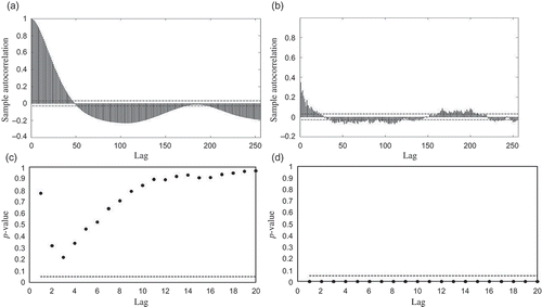
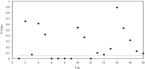
Trying different models with different parameter orders, the best model is selected based on the minimum Akaike Information Criterion (AIC) and testing the residuals of the model for adequacy. Therefore, an ARIMA (13,1,4) model is fitted to daily time series of the Matapedia River. The p values of the Ljung-Box goodness-of-fit test (Fig. 1(c)) indicate the adequacy of the above model as all p values are above the critical level (α = 0.05). Then, we apply the Engle test for testing the ARCH effect in the residuals. As shown in Fig. (1(d)) for the first 20 lag times, all p values of the Engle test are less than the critical level and therefore the existence of an ARCH effect in the residuals of the ARIMA (13,1,4) model is verified. Hence, a GARCH model should be applied to capture and remove the heteroscedasticity remaining in the residuals of the ARIMA (13,1,4) model.

5.2 GARCH model

It was illustrated in the previous section that the heteroscedasticity of the residuals of the ARIMA model is significant and we need to fit a GARCH model to capture the conditional variance of the residuals. The three types of GARCH models presented in Section 2.2 are fitted to the residuals of the ARIMA model.

5.2.1 Power GARCH model

The first model fitted to the residuals of the ARIMA model is the PGARCH (3,1) model. The PGARCH (3,1) model for the residuals of the ARIMA model can be written as:

(18)

Thus, we have an ARIMA (13,1,4)-PGARCH (3,1) error model for streamflow data with δ = 2.35. For the above model, all parameters are significant at the 95% level and the model is selected according to the minimum AIC.

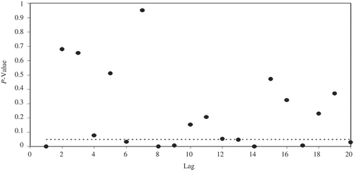
In order to check the ARCH effect of the residuals of the above model, the Engle test is applied. The p values of the test are given in Fig. 2, which illustrates the advantage of a PGARCH model against the ARIMA model as most of the p values are larger than the critical value and the ARCH effect has been significantly reduced. However, some p values are still below the critical value for some lags which indicates some ARCH effect in the residuals. Therefore, one can conclude that the PGARCH model has not completely removed the heteroscedasticity from the residuals of the ARIMA model.

Fig. 2 p values of the Engle test for SSRs of the ARIMA-PGARCH error model.

5.2.2 Threshold GARCH model

The threshold GARCH model can take into account the effect of the negative and positive errors of the ARIMA model on the conditional variance of the residuals. The TGARCH (3,1) model can be fitted to the residuals of the ARIMA model according to the minimum AIC and can be written as:

(19)

In this model, as , we can conclude that the negative error (observed – estimated < 0) and the positive error (observed – estimated > 0) of the ARIMA model have an asymmetric impact on the volatility or the heteroscedasticity of the residuals. However, it is said in finance that as γ > 0, bad news, or ε < 0, increases the volatility. In our case, an example in hydrology, we can say that over-estimation of an ARIMA model, or negative errors when “observed – estimated = residuals < 0”, will increase the heteroscedasticity in the residuals. Looking at the residuals of the ARIMA model indicates that 61% of the errors are over-estimations (negative errors) and 39% of the errors are under-estimations (positive errors), which may result in the asymmetric characteristic of the residuals for which a TGARCH has been fitted. In other words, the heteroscedasticity of the residuals of the ARIMA model of streamflow time series comes from over-estimation rather than under-estimation.

To check the efficiency of heteroscedasticity modelling, the ARCH effect of the residuals of the ARIMA-TGARCH model is examined by the Engle test. The p values of the test are given in Fig. 3. Similar to the PGARCH model, Fig. 3 also shows a significant reduction in the heteroscedasticity of the ARIMA-TGARCH model compared to the ARIMA model. However, some p values are still below the critical value at some lag times (e.g. K = 1, 6, 8, 9, 14, 17 and 20), and it seems that the heteroscedasticity still exists in the residuals and the TGARCH model is not adequate for capturing all heteroscedasticity of the residuals.

Fig. 3 p values of the Engle test for SSRs of the ARIMA-TGARCH error model.

5.2.3 Exponential GARCH model

The EGARCH model is a GARCH model for the logarithm of the conditional variance. Fitting an EGARCH (3,1) to the residuals of the ARIMA (13,1,4) model will give the following model:

(20)

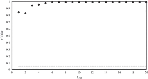
All the parameters of the model are significant at the 95% level. The existence of an ARCH effect in the residuals of the ARIMA (13,1,4)-EGARCH (3,1) model is examined by the Engle test. The p values of the test are given in Fig. 4. It is clear that all p values are above the critical level of rejecting the null hypotheses of the ARCH effect and one can conclude that no ARCH effect remains in the residuals of the ARIMA-EGARCH error model. We can also see that the EGARCH model is much better than the PGARCH and TGARCH models in capturing the conditional variance of the residuals of the ARIMA model. This may be due to fact that the EGARCH model considers the logarithm of the variance of the residuals.

Fig. 4 p values of the Engle test for SSRs of the ARIMA-EGARCH error model.

5.3 Model evaluation

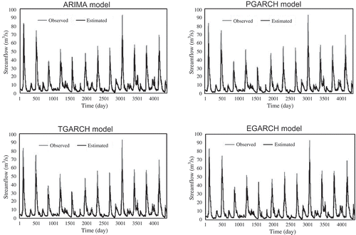
The performance of the time series models presented in the previous sections is assessed here by applying criteria that evaluate the errors of the model. Before considering the criteria, we first look at the scatter plots and time series plots of the observed against estimated streamflow time series in Figs 5 and 6.

Fig. 5 Scatter plot of observed against estimated streamflows for different models.

Fig. 6 Time series plot of observed and estimated streamflows for different models.

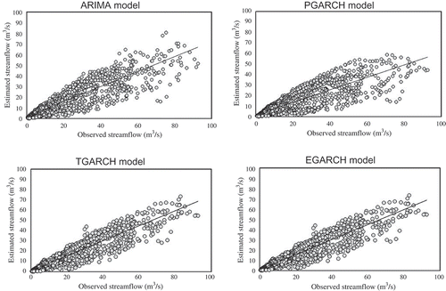
The scatter plots of the observed against estimated streamflow time series (Fig. 5) indicate that all the models are weak in estimating the high flows, but their performance is good in estimation of low flows. The cloud of observations of high flows indicates that the performance of the ARIMA model and PGRCH and TGARCH models are almost the same. The variation of high flow observations for the EGARCH model, however, reveals the best performance among the models as the distribution of the observations around the best fit line is closest. The time series plots of the observed and estimated streamflows, given in Fig. 6, also confirm that the EGARCH model has the best performance among the models. However, the numerical criteria are used and discussed to evaluate the model performance.

5.3.1 Multi-criteria evaluation

The evaluation and comparison of the time series models is carried out through the application of the criteria listed in Section 3.1 and are presented in Table 1. It is observed that the performance of an ARIMA model is better than the PGARCH and TGARCH models according to both the error and dimensionless criteria. The error in peak flow estimation for the ARIMA model is also less than that of the PGARCH and TGARCH models, which implies that the ARIMA model is more efficient for estimating the maximum flow than the GARCH models. It is clear from Table 1 that the EGARCH model is best model among the models fitted to the streamflow time series. All the criteria, except PDIFF, demonstrate the better performance of the EGARCH model. The error criteria, MAE, RAE and RMSE, indicate relatively less error for the EGARCH model than other models. According to R ², the EGARCH model describes 93% of the variation of the observed streamflow. Therefore, the EGARCH model can be considered as “very satisfactory”, based on the model efficiency classification of R² given by Dawson et al. (2007). The other models are considered as “good” models according to their R ² values.

Table 1  Evaluation criteria for time series models (italics indicate result is significant)

Criteria	Models
	ARIMA	PGARCH	TGARCH	EGARCH
AME	54.34	58.23	58.33	42.11
PDIFF	11.44	33.7	32.25	19.33
MAE	2.46	2.93	2.92	2.03
RMSE	5.66	7.15	7.1	4.86
RAE	0.27	0.32	0.32	0.22
R ^2 (%)	86	81	81	93
IoAd (%)	94	89	90	96

The PDIFF is the only measurement for which the ARIMA model performs better than the EGARCH model. This measurement indicates the difference between a (single) maximum value in the observed data set and a (single) maximum value in the estimated data set and cannot reflect the overall performance of a model. The scatter plots show also that the general agreement between observed and estimated high flows is better in the EGARCH model than the ARIMA model. Therefore, the EGARCH model is selected as the best model among the time series models applied in this study.

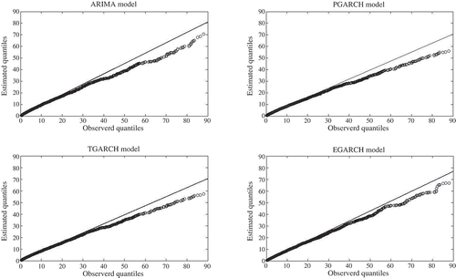
5.3.2 QQ plot

The QQ plots of the time series models are given in Fig. 7. These show that all models underestimate the high streamflow quantiles, but the low streamflow quantiles are better estimated. It is worth noting that the departure of estimated quantiles from the observed ones is almost the same for the ARIMA, PGARCH and TGARCH models. All models show a difference between observed and estimated streamflow for values that range between 40 and 60 m³/s. This difference increases for higher quantiles (streamflow > 60 m³/s). For the EGARCH model, however, the departure of quantiles from the y = x line is smaller than the other models for both medium and high quantiles. This represents one of the advantages of using the appropriate GARCH model: reduction of the variation of the model output and reduction of the uncertainty of model estimation. The small departure of the EGARCH model may also be due to the logarithm transformation of the variance of the residuals of the ARIMA model.

Fig. 7 QQ plots of time series models.

6 CONCLUSIONS

The conditional variance or the time-dependent variance of hydrological variables is usually ignored in hydrological time series modelling. This study illustrates the advantages of the application of a nonlinear GARCH approach for modelling the variance of streamflow time series. The ARMA-GARCH error model presented in this study includes the common ARMA or ARIMA model for modelling the conditional mean of streamflows, while the GARCH approach models the conditional variance remaining in the residuals of the ARMA or ARIMA model. Engle's test confirms that the variance of the residual of the linear model is not homoscedastic and shows time varying features.

Three types of asymmetric GARCH model, the Power GARCH, Threshold GARCH and exponential GARCH models, already applied in financial sciences, are introduced and applied here for modelling the time varying variance of daily streamflows. These three models are based on asymmetric behaviour of the conditional variance of a financial variable.

Though the GARCH models show the advantage of reducing the heteroscedasticity of the residuals of the ARIMA model, the performances of the Power GARCH and Threshold GARCH models are not better than the linear ARIMA model. However, the exponential GARCH model outperforms the ARIMA model and other GARCH models. The better performance of the EGARCH model may be due to the fact that the exponential GARCH model considers the logarithm of the variance of the residuals which may lead to a stabilization of variance and reduces the error of the model. Apart from the effect of the logarithm transformation, no specific reason was indicated in the financial literature (e.g. Tavares et al. 2008, Miron and Tudor 2010), for a better performance of the EGARCH model against PGARCH and TGARCH models fitted to different financial time series, except that the data “speaks” and help us to decide which model is the best model (J.D. Curto 2012, personal communication). Therefore, we need to apply different hydrological variables to examine the suitability of different asymmetric GARCH models in hydrology, climatology and water resources.

Another important result is related to the significant parameter of a Threshold GARCH model which verifies the asymmetric effect of negative and positive errors on the remaining heteroscedasticity in the residuals of an ARIMA model. The effect of asymmetry on the heteroscedasticity is a well-known concept in financial time series modelling but it has not received enough attention in hydrology. In this study it was observed that the negative errors of the ARIMA model (or the over-estimation) will increase the heteroscedasticity in the residuals of a linear model. In other words, over-estimation causes more heteroscedastic residuals than under-estimation. Consequently GARCH models can be considered as a serious alternative in hydrology when over-estimation occurs. The asymmetric effect of the residuals of the ARIMA model on the conditional variance of the residuals could also be a promising topic for future studies in hydrology and water resources.

Finally, the results of our case study suggest the advantages of an appropriate/some GARCH-type models for both capturing the heteroscedasticity in the residuals of the linear time series models and improving the efficiency of the models. As few studies have applied nonlinear GARCH models in hydrology, it is hoped that future work will focus on the application of these models to other hydrological and climatic variables, such as rainfall and temperature at different time scales using different GARCH models. Although the PGARCH and TGARCH models do not show an advantage over ARIMA model for our streamflow data, they may show their advantages for other hydrological time series with different conditional variance temporal characteristics.

Acknowledgements

The authors would like to thank the Natural Sciences and Engineering Research Council (NSERC) of Canada and the Canada Research Chair (CRC) Program for financially supporting this work.

REFERENCES

- Bollerslev , T. 1986 . Generalized autoregressive conditional heteroscedasticity . Journal of Econometrics , 31 : 307 – 327 .
- Chen , C.H. , Liu , C.H. and Su , H.C. 2008 . A nonlinear time series analysis using two-stage genetic algorithms for streamflow forecasting . Hydrological Processes , 22 : 3697 – 3711 .
- Chen , H.L. and Rao , A.R. 2003 . Linearity analysis on stationary segments of hydrologic time series . Journal of Hydrology , 277 : 89 – 99 .
- Dawson , C.W. , Abrahart , R.J. and See , L.M. 2007 . Hydrotest: a web-based toolbox of evaluation metrics for the standardized assessment of hydrological forecasts . Environmental Modelling & Software , 22 : 1034 – 1052 .
- Ding , Z. , Grangerand , C.W.J. and Engle , R.F. 1993 . A long memory property of stock market returns and a new model . Journal of Empirical Finance , 1 : 83 – 106 .
- Engle , R.F. 1982 . Autoregressive Conditional Heteroscedasticity with estimates of variance of United Kingdom inflation . Econometrica , 50 : 987 – 1008 .
- Francq , C. and Zakoian , J.M. 2010 . GARCH models structure, statistical inference and financial applications , Chichester : John Wiley & Sons Ltd .
- Hipel , K.W. and McLeod , A.E. 1996 . Time series modeling of water resources and environmental systems , Amsterdam : Elsevier .
- Kurunc , A. , Yurekli , K. and Cevik , O. 2005 . Performance of two stochastic approaches for forecasting water quality and streamflow data from Yesilirmak River, Turkey . Environmental Modeling and Software , 20 : 1195 – 1200 .
- Machiwal , D. and Jha , M. 2008 . Comparative evaluation of statistical tests for time series analysis: application to hydrological time series . Hydrological Sciences Journal , 53 : 353 – 366 .
- Miron , D. and Tudor , C. 2010 . Asymmetric conditional volatility models: empirical estimation and comparison of forecasting accuracy . Romanian Journal of Economic Forecasting , 13 ( 3 ) : 74 – 92 .
- Modarres , R. 2007 . Streamflow drought time series forecasting . Stochastic Environmental Research and Risk Assessment , 21 ( 3 ) : 223 – 233 .
- Modarres , R. 2009 . Multi-criteria validation of artificial neural network rainfall--runoff modeling . Hydrology and Earth System Sciences , 13 : 411 – 421 .
- Nelson , D.B. 1991 . Conditional heteroskedasticity in asset returns: a new approach . Econometrica , 69 : 1519 – 1554 .
- Ouarda , T.B.M.J. , Labadie , J.W. and Fontane , G. 1997 . Indexed sequential hydrologic modeling for hydropower capacity estimation . Journal of the American Water Resources Association , 33 : 1 – 13 .
- Rao , A.R. and Yu , G.H. 1990 . Gaussianity and linearity tests of hydrologic time series . Stochastic Hydrology and Hydraulics , 4 : 121 – 134 .
- Tavares , A.B. , Curto , J.D. and Tavares , G.N. 2008 . Modeling heavy tails and asymmetry using ARCH-Type models with stable Paretian distribution . Nonlinear Dynamics , 51 : 231 – 243 .
- Toth , E. , Montanari , A. and Brath , A. 1999 . Real-time flood forecasting via combined use of conceptual and stochastic models . Physics and Chemistry of the Earth (B) , 24 : 793 – 798 .
- Wang , W. 2006 . Stochasticity, nonlinearity and forecasting of streamflow processes , Amsterdam : Delft University Press .
- Wang , W. 2005 . Testing and modeling autoregressive conditional heteroskedasticity of streamflow processes . Nonlinear Process in Geophysics , 12 : 55 – 66 .
- Wang , W. 2006 . Testing for nonlinearity of streamflow processes at different timescales . Journal of Hydrology , 322 : 247 – 268 .
- Zakoïan , J.M. 1994 . Threshold heteroskedastic models . Journal of Economic Dynamics Control , 18 : 931 – 944 .