Hydrology and change

Abstract

Since “panta rhei” was pronounced by Heraclitus, hydrology and the objects it studies, such as rivers and lakes, have offered grounds to observe and understand change and flux. Change occurs on all time scales, from minute to geological, but our limited senses and life span, as well as the short time window of instrumental observations, restrict our perception to the most apparent daily to yearly variations. As a result, our typical modelling practices assume that natural changes are just a short-term “noise” superimposed on the daily and annual cycles in a scene that is static and invariant in the long run. According to this perception, only an exceptional and extraordinary forcing can produce a long-term change. The hydrologist H.E. Hurst, studying the long flow records of the Nile and other geophysical time series, was the first to observe a natural behaviour, named after him, related to multi-scale change, as well as its implications in engineering designs. Essentially, this behaviour manifests that long-term changes are much more frequent and intense than commonly perceived and, simultaneously, that the future states are much more uncertain and unpredictable on long time horizons than implied by standard approaches. Surprisingly, however, the implications of multi-scale change have not been assimilated in geophysical sciences. A change of perspective is thus needed, in which change and uncertainty are essential parts.

Editor Z.W. Kundzewicz

Citation Koutsoyiannis, D., 2013. Hydrology and change. Hydrological Sciences Journal, 58 (6), 1177–1197.

Résumé

Depuis que “panta rhei” fut prononcé par Héraclite, l’hydrologie et les objets qu’elle étudie, comme les rivières et les lacs, offrent des champs d’observation et de compréhension du changement et des flux. Le changement se produit à toutes les échelles de temps, de la minute aux durées géologiques, mais la limitation de nos sens et de la durée de nos vies, de même que l’étroitesse de la fenêtre des observations instrumentales, restreignent notre perception aux variations les plus évidentes, quotidiennes et annuelles. En conséquence, nos pratiques habituelles en matière de modélisation supposent que les changements naturels ne sont qu’un “bruit” à court terme se superposant aux cycles quotidiens ou annuels sur une scène statique et invariable à long terme. Selon cette perception, seul un forçage exceptionnel et extraordinaire peut produire un changement à long terme. L’hydrologue H.E. Hurst, en étudiant les longues séries de débit du Nil et d’autres séries chronologiques géophysiques, fut le premier à observer un comportement naturel, auquel son nom a été donné, lié à des changements d’échelles multiples, ainsi qu’à en tirer des conséquences au niveau de la conception des ouvrages. Essentiellement, ce comportement montre que des changements à long terme sont beaucoup plus fréquents et plus intenses qu’on ne le perçoit généralement et, également, que l’avenir à long terme est beaucoup plus incertain et imprévisible que ce que supposent les approches classiques. Étonnamment, cependant, les implications des changements d’échelles multiples n’ont pas été assimilées dans les sciences géophysiques. L’adoption d’une nouvelle perspective est donc nécessaire, dans laquelle le changement et l’incertitude seront des éléments essentiels.

Key words:

• hydrology
• change
• turbulence
• Hurst-Kolmogorov behaviour
• uncertainty

Mots clefs:

• hydrologie
• changement
• turbulence
• comportement de Hurst-Kolmogorov
• incertitude

“Both classical physics and quantum physics are indeterministic”

(Karl Popper, in his book Quantum Theory and the Schism in Physics)

“The future is not contained in the present or the past”

(W. W. Bartley III, in Editor’s Foreword to the same book)

INTRODUCTION

To save several thousands of words, the explanation of the subject of this essay is based on some pictures grouped as Figs 1 and 2. Figure 1 provides a pictorial illustration of the domain of hydrology, whose definition as a modern science was established about half a century ago by UNESCO (1963, 1964; complementing an earlier definition by a US Ad Hoc Panel on Hydrology, 1962):

“Hydrology is the science which deals with the waters of the earth, their occurrence, circulation and distribution on the planet, their physical and chemical properties and their interactions with the physical and biological environment, including their responses to human activity.”

Fig. 1 Pictorial illustration of the domain of hydrology using photographs taken from space and made available by NASA. In clockwise order, starting from top left: (a) view of the Earth and its water in the form of oceans, ice in Antarctica and clouds (a classic photograph known as the “Blue Marble” of the Earth taken by the Apollo 17 crew travelling toward the moon on 7 December 1972); (b) the northern portion of the Nile River; (c) the Nile River Delta and the Mediterranean at night; (d) the Aswan High Dam on the Nile; (e) the Lake Nasser in Egypt, upstream of the dam. All photographs are copied from earthobservatory.nasa.gov/IOTD/view.php?id=xxxx, where xxxx = 1133, 1234, 46820, 2416 and 5988 for (a)–(e), respectively.

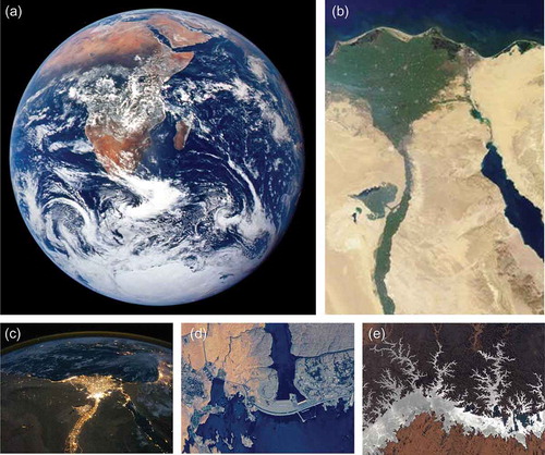
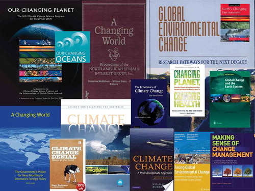
Fig. 2 A collage of covers of recent books focusing on change.

As illustrated in Fig. 1, hydrology embraces the full cycle of water on the Earth in all its three phases. The domain of hydrology spans several temporal and spatial scales. Of course, large hydrological systems, such as the Nile River, are of huge importance. The image of the Nile also highlights the connection of water with life: the blue colour of the Nile is not seen, but one can see the green of the life it gives rise to. The contrast of green with the desert beige demonstrates that life is concentrated near the water of the Nile. During the night, the green areas turn into brightly lit areas, indicating the relationship of human civilization with water bodies (the population is almost completely concentrated along the Nile Valley), and the absence thereof with dark. The focus on the Aswan High Dam on the Nile emphasizes the strong link of hydrology with engineering, and through this, with the improvement of diverse aspects of our lives and civilization. (When completed, the hydropower stations of the dam provided half of the electricity of Egypt.) The next focus, on Lake Nasser, upstream of the Aswan Dam, indicates that the intervention of humans on Nature can really be beautiful.

Figure 2 indicates that the title of this paper, “Hydrology and change”, harmonizes with a large body of literature, books, conferences, scientific papers and news stories, all of which roar about change: changing planet, changing world, changing ocean, changing environment, changing health and, most of all, changing climate. It looks as if, recently, our scientific community has been amazed that things change.

SOME HISTORICAL NOTES ON THE PERCEPTION OF CHANGE

In reality, change has been studied since the birth of science and philosophy. Most of the Greek philosophers had something to say about it. The following quotations by two of them, Heraclitus (ca. 540–480 BC) and Aristotle (384–322 BC) are fascinating examples.

Heraclitus summarized the dominance of change in a few famous aphorisms, in which he uses simple hydrological notions to describe change: the flow and the river. Most famous is an aphorism no longer than two words, magically put together: Everything flows (better known in its original Greek version, “”)¹. Alternative expressions of the same idea are: “All things move and nothing remains still”²; “Everything changes and nothing remains still”³; and “You cannot step twice into the same river”.⁴

It is amazing that Aristotle (particularly in his Meteorologica) understood the scale and extent of change much better than some contemporary scholars do:

Neither the Tanais [River Don in Russia] nor the Nile have always been flowing, but the region in which they flow now was once dry: for their life has a bound, but time has not [. . .] But if rivers are formed and disappear and the same places were not always covered by water, the sea must change correspondingly. And if the sea is receding in one place and advancing in another it is clear that the same parts of the whole earth are not always either sea or land, but that all changes in course of time.⁵

He also understood and aptly expressed the conservation of mass within the hydrological cycle (cf. Koutsoyiannis et al. 2007): “Thus, [the sea] will never dry up; for [the water] that has gone up beforehand will return to it”⁶ and “Even if the same amount does not come back every year or in a given place, yet in a certain period all quantity that has been abstracted is returned.”⁷

Given this ancient knowledge, the current inflationary focus on change, as illustrated in Fig. 2, is puzzling. Undoubtedly, change has been accelerated in modern times due to radical developments in demography, technology and life conditions. This acceleration, however, does not fully resolve the puzzle; for example it does not explain the generally negative view of change by society, whilst most technology-enabled changes in our lives are desirable, intended and positive. Therefore, additional questions about the modern social perception of change arise. Did we miss our perception and knowledge of change and are we trying to reinvent them? Or has our society lost its ability to adapt to change, so that we became apprehensive? Or, even worse, has our society become so conservative as to worry that things change?

Useful information that helps to investigate and quantify our perception of change has been provided recently by the Google Ngram Viewer, a phrase-usage graphing tool, which charts the frequency per year of selected n-grams (letter combinations, i.e. words, or phrases), as found in several million books digitized by Google (up to 2008; books.google.com/ngrams; see also Michel et al. 2011). Note that the frequencies are relative, i.e. for each year, the frequency of a specified n-gram is the ratio of the number of appearances of that n-gram to the number of all n-grams in books published in that year and contained in the Google collection. Using this viewer, one can readily see that the frequency of the use of the word “change” has more than doubled from 1800 to the present, and that of “changing” has more than tripled.

However, it is more interesting to investigate phrases related to major changes such as those appearing in Fig. 2. Some informative graphs are given in Fig. 3, where we can see that, from about 1900, people started to speak about a “changing world” and a little later about “environmental change”. The use of “demographic change”, “climate change” and “global change” starts in the 1970s and 1980s. If we assume that the intense use of these expressions reflects fears or worries about change, we may conclude that such worries have receded since 2000, except one: climate change. It is interesting that, since the late 1980s, “climate change” dominated over “environmental change” and “demographic change”. This harmonizes with a more general political, ideological and economic trend of our societies to give more importance to speculations, hypotheses, scenarios and virtual reality instead of facing the facts (cf. Koutsoyiannis et al. 2009).

Fig. 3 Evolution of the frequency per year of the indicated phrases related to major changes, as found in several million books digitized by Google covering the period from the beginning of the 19th century to present (the data from 360 billion words contained in 3.3 million books published after 1800 and the graphs are provided by Google ngrams; books.google.com/ngrams).

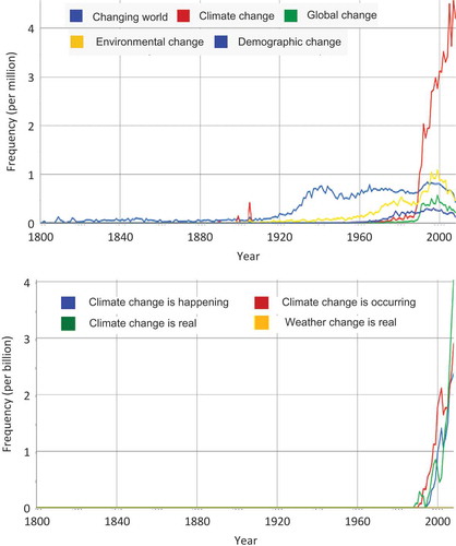
Indeed, the demographic and environmental changes of the 20th century are unprecedented and determinant, while it is well known (see also below) that climate has been in perpetual change throughout Earth’s existence. It is thus hilarious to read, increasingly often, as shown in the lower panel of Fig. 3, statements like “climate change is happening”, “. . . is occurring” and “. . . is real”. These statements contain the same truth and value as “weather change is real”, but no appearance of the latter in books has been reported.

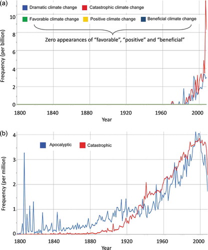
Figure 4 gives some additional information useful for understanding the reasons for current dominant ideas and trends. Specifically, “climate change” is only presented as “negative” or “catastrophic”, while adjectives like “positive”, “favourable” and “beneficial” have never been combined with “climate change”. Is change really only negative? Even removing “climate” or “climate change” from our phrases, we can see (lower panel of Fig. 4, depicting the frequency of the words “apocalyptic” and “catastrophic”) that our societies are becoming more and more susceptible to fear, pessimism and guilt (cf. Christofides and Koutsoyiannis 2011). Apparently, such feelings and ideologies provide ideal grounds for political and economic interests related to the “climate change” agenda.

Fig. 4 Evolution of the frequency per year of the indicated phrases related to pessimistic views, as found in several million books digitized by Google covering the period from the beginning of the 19th century to present (data and graphs by Google ngrams; books.google.com/ngrams).

PREDICTABILITY AND CHANGE

The hierarchical chart of Fig. 5 tries to classify change with respect to its predictability. In simple systems (left part of the graph) the change is regular. The regular change can be periodic or aperiodic. Whatever it is, using equations of dynamical systems, regular change is predictable. But this type of change is rather trivial. More interesting are the more complex systems with long time horizons (right part of the graph), where change is unpredictable in deterministic terms, or random. Pure randomness, such as in classical statistics, where different variables are identically distributed and independent, is sometimes a useful model, but in most cases it is inadequate. A structured randomness should be assumed instead. As will be seen next, the structured randomness is enhanced randomness, expressing enhanced unpredictability of enhanced multi-scale change.

Fig. 5 Classification of change with respect to predictability.

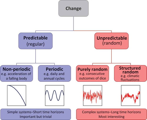
Here it should be clarified that the concept of randomness is used herein with a meaning different from the most common. According to the common dichotomous view, natural processes are composed of two different, usually additive, parts or components—deterministic (signal) and random (noise). At large time scales, randomness is cancelled out and does not produce change. Thus, according to the common view, only an exceptional forcing can produce a long-term change. In contrast, in the view adopted here and better explained in Koutsoyiannis (2010), randomness is none other than unpredictability. Randomness and determinism coexist and are not separable. Deciding which of the two dominates is simply a matter of specifying the time horizon and scale of the prediction. For long time horizons (where the specific length depends on the system), all is random—and not static.

Interestingly, Heraclitus, who became known mostly for his apophthegms about change, also pronounced that randomness dominates: “Time is a child playing, throwing dice.”⁸ Such a view was also promoted by Karl Popper, as reflected in the motto at the beginning of this paper. However, excepting quantum physics, the dominant scientific view still identifies science with determinism and banishes randomness as an unwanted “noise”. In antithesis to Heraclitus, Albert Einstein’s aphorism, “I am convinced that He does not throw dice”⁹ has been the emblem of the dominance of determinism in modern science.

One can argue that not only does God play dice but He wants us to be aware of His dice game without having to wait too long: turbulence may be one of His favourite dice games as we can see it visually, just looking at any flow (Fig. 6), but we can also take quantified measurements at very fine time scales (Fig. 7). Turbulence is a very complex phenomenon; according to a saying attributed to Werner Heisenberg or, in different versions, to Albert Einstein or to Horace Lamb: “When I meet God, I am going to ask him two questions: Why relativity? And why turbulence? I really believe He will have an answer for the first.”

Fig. 6 Flood in the Arachthos River, Epirus, Greece, under the medieval Bridge of Arta, in December 2005. The bridge is famous from the legend of its building, transcribed in a magnificent poem (by an anonymous poet) symbolizing the dedication of the engineering profession and the implied sacrifice; see en.wikisource.org/wiki/Bridge_of_Arta.

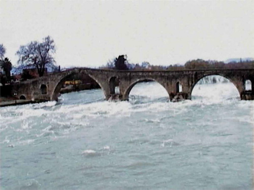
Fig. 7 (a) Laboratory measurements of nearly isotropic turbulence in Corrsin Wind Tunnel at a high Reynolds number (Kang et al. 2003). (b) A purely random synthetic time series with mean and standard deviation equal to those in (a); the different values are realizations of independent identically distributed random variables with Gaussian distribution.

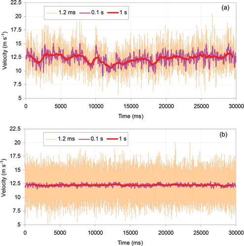
In Fig. 7(a), which visualizes the velocity fluctuations in a turbulent flow, each data point represents the average velocity every 1.2 ms, while time averages at time scales of 0.1 and 1 s are also plotted. The data are measurements by X-wire probes with a sampling rate of 40 kHz (here aggregated at 0.833 kHz) from an experiment at the Corrsin Wind Tunnel (section length 10 m; cross-section 1.22 m × 0.91 m) at a high Reynolds number (Kang et al. 2003; data available online at http://www.me.jhu.edu/meneveau/datasets/Activegrid/M20/H1/m20h1-01.zip).

To understand the change encapsulated in turbulence, we compare the graph of turbulent velocity measurements (Fig. 7(a)) with pure random noise (also known as white noise) with the same statistical characteristics at the lowest time scale (Fig. 7 (b)). The differences are substantial. If we adopted the widespread dichotomous views of phenomena mentioned in the beginning of this section, we would say that in the turbulent signal we see some structures or patterns, suggestive of long-term change, which could be interpreted as a deterministic behaviour (e.g. deterministic trends etc.). Yet, such patterns do not appear in the purely random process (white noise). In this interpretation, the turbulent series is a synthesis of a random and a deterministic component, while the white noise series is purely random and thus more random than the turbulent signal.

However, this interpretation is incorrect. The patterns seen in turbulence are unpredictable in deterministic terms and thus could not classify as deterministic. Instead, according to the above view, in which randomness is none other than unpredictability, the patterns in turbulence are random. In pure randomness (white noise) there are no long-term patterns; rather, the time series appears static in the long run. Structured randomness (in turbulence), in addition to short-term irregular fluctuations, which are a common characteristic with pure randomness, also exhibits long-term random patterns. The two time series shown in Fig. 7(a) and (b) have exactly the same variability at the lowest scale, 1.2 ms, but their behaviour becomes different at larger scales. Specifically, at scales of 0.1 and 1 s, pure randomness does not produce any variability or change. In turbulence, change is evident also at these scales. This change is unpredictable in deterministic terms and thus random and, more specifically, structured (or enhanced) random rather than purely random.

Following Heraclitus, who associated change with river flow, we can contemplate the simply understood changes in a river, considering phenomena from mixing and turbulence, to floods and droughts and going beyond those, by imagining time horizons up to millions of years:

• Next second: the hydraulic characteristics (water level, velocity) will change due to turbulence;

• Next day: the river discharge will change (even dramatically, in case of a flood);

• Next year: the river bed will change (erosion–deposition of sediments);

• Next century: the climate and the river basin characteristics (e.g. vegetation, land use) will change;

• Next millennium: all could be very different (e.g. the area could be glacierized);

• Next millions of years: the river may have disappeared.

None of these changes will be a surprise; rather, it would be a surprise if things remained static. Despite being anticipated, none of these changes are predictable in deterministic terms. Even assuming that the mechanisms and dynamics producing these changes are perfectly understood, the changes remain unpredictable at the indicated time horizons for each of the above types of change (though at smaller times the dynamics may enable deterministic predictability; see Koutsoyiannis 2010). Furthermore, most of these changes can be mathematically modelled in a stochastic framework admitting stationarity!

QUANTIFICATION OF CHANGE IN STOCHASTIC TERMS

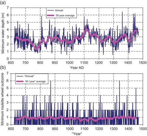
While the time series of turbulence shown in Fig. 7 can be used to quantify change at scales of up to several seconds, we certainly need much longer time series to quantify the changing behaviour of natural processes at scales relevant to everyday life. The longest instrumental record is that of the water level of the Nile. The observations were taken at the Roda Nilometer, near Cairo (Fig. 8). Toussoun (1925) published the annual minimum and maximum water levels of the Nile at the Roda Nilometer from AD 622 to 1921. During 622–1470 (849 years), the record is almost uninterrupted, but later there are large gaps. The annual minimum water levels of this period are plotted in Fig. 9 along with their 30-year averages. The latter are commonly called climatic values, and, due to the large extent of the Nile basin, they reflect the climate evolution of a very large area in the tropics and subtropics. We may notice that around AD 780 the climatic (30-year) minimum value was 1.5 m, while in AD 1110 and 1440 it was 4 m, 2.5 times higher. In Fig. 9(b), we can see a simulated series from a roulette wheel which has equal variance to the Nilometer. Despite having equal “annual” variability, the roulette wheel produces a static “climate”.

Fig. 8 The Roda Nilometer, near Cairo, as it stands today; water entered through three tunnels and filled the Nilometer chamber up to river level (Photos: Aris Georgakakos).

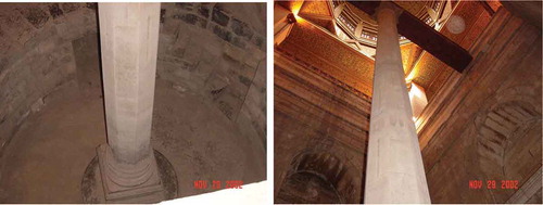
Fig. 9 (a) Nile River annual minimum water depth at Roda Nilometer (849 values from Toussoun 1925, here converted into water depths assuming a datum for the river bottom of 8.80 m); a few missing values for years 1285, 1297, 1303, 1310, 1319, 1363 and 1434 are filled in using a simple method from Koutsoyiannis and Langousis (2011; p. 57). (b) Synthetic time series, each value of which is the minimum of m = 36 roulette wheel outcomes; the value of m was chosen so that the standard deviation equals that of the Nilometer series (where the latter is expressed in metres).

The first person to notice this behaviour, and in particular the difference between natural processes and purely random processes, was the British hydrologist H. E. Hurst, who worked on the Nile for 60 years. His motivation was the design of hydraulic projects on the Nile (Fig. 1), but his seminal paper (Hurst 1951) was theoretical and explored numerous data sets of diverse fields. He emphasized the clustering or grouping of similar events in natural processes: “Although in random events groups of high or low values do occur, their tendency to occur in natural events is greater. This is the main difference between natural and random events.”

This grouping of similar events is another way to describe long-term change. While Hurst’s discovery is more than 60 years old, it has not been well disseminated, let alone assimilated and adopted by the wider scientific community, yet. Obstacles in the dissemination were, inter alia, Hurst’s use of a complicated statistic (the rescaled range), directly connected with reservoir storage, and the focus on the Nile.

Strikingly, 10 years earlier, the Soviet mathematician and physicist A. N. Kolmogorov—a great mind of the 20th century, who gave probability theory its modern foundation and also studied turbulence—had proposed a mathematical process that has the properties which were discovered 10 years later by Hurst in natural processes (Kolmogorov 1940). Here, we call this the Hurst-Kolmogorov (or HK) process, although the original name given by Kolmogorov was “Wiener’s spiral”, and it later became more widely known by names such as “self-similar process”, or “fractional Brownian motion” (Mandelbrot and van Ness 1968). Kolmogorov’s work did not become widely known, but the proof of the existence of this process is important, because several researchers, ignorant of Kolmogorov’s work, regarded Hurst’s finding as inconsistent with stochastics and as a numerical artefact.

The mathematics to describe the HK process is actually very simple and the calculations can be done in a common spreadsheet. No more than the concept of standard deviation from probability theory is needed. Because a static system whose response is a flat line (no change in time) has zero standard deviation, we could recognize that the standard deviation is naturally related to change. To study change, however, we need to assess the standard deviation at several time scales.

Let us take as an example the Nilometer time series, x₁, x₂, . . ., x₈₄₉, and calculate the sample estimate of standard deviation σ(1), where the argument (1) indicates a time scale of 1 year. We form a time series at time scale 2 (years):

(1)

and calculate the sample estimate of standard deviation σ(2). We proceed forming a time series at time scale 3 (years):

(2)

and we calculate the sample estimate of standard deviation σ(3). We repeat the same procedure up to scale 84 (years):

(3)

and calculate σ(84). Here, the maximum scale k_max = 84 is 1/10 of the record length; in theory the procedure could be repeated up to k_max = 424, in which case we would calculate a series with two elements; this would give an estimate of standard deviation σ(424), but it has been deemed (e.g. Koutsoyiannis 2003, Koutsoyiannis and Montanari 2007, Koutsoyiannis, 2013) that 10 data points, as in (3), is a minimum to provide a reliable estimate of the standard deviation.

The logarithmic plot of standard deviation σ(k) vs scale k, which has been termed the climacogram, is a very informative tool. If the time series x_i represented a purely random process, the climacogram would be a straight line with slope –0.5, as implied by the classical statistical law:

(4)

In real-world processes, the slope is different from –0.5, designated as H – 1, where H is the so-called Hurst coefficient. This slope corresponds to the scaling law:

(5)

which defines the Hurst-Kolmogorov (HK) process. It can be seen that if H > 1, then σ(k) would be an increasing function of k, which is absurd (averaging would increase variability, which would imply autocorrelation coefficients >1). Thus, the Hurst coefficient is restricted in the interval 0.5 ≤ H < 1. The value 0.5 corresponds to white noise (equation (5) switches to (4)). Values H < 0.5, characteristic of anti-persistence, are mathematically feasible (in discrete time) but physically unrealistic; specifically, for 0 < H < 0.5 the autocorrelation for any lag is negative, while for small lags a physical process should necessarily have positive autocorrelation. High values of H, particularly those approaching 1, indicate enhanced change at large scales or strong clustering (grouping) of similar values, otherwise known as long-term persistence. In other words, in a stochastic framework and in stationary terms, change can be characterized by the Hurst coefficient.

It should be noted that the standard statistical estimator of standard deviation σ, which is unbiased for independent samples, becomes biased for a time series with HK behaviour. The bias can be predicted (Koutsoyiannis 2003, Koutsoyiannis and Montanari 2007). It is thus essential that, if the sample statistical estimates are to be compared with model (5), the latter must have been adapted for bias before the comparison.

Equation (5) corresponds to a stochastic process in discrete time, in which k is dimensionless (representing the number of time steps for aggregation, and in our example number of years). For completeness, the continuous time version is:

(6)

where a is any time scale, σ(a) is the standard deviation at scale a, and both a and k have units of time.

Another stochastic process commonly used in many disciplines is the Markov process, whose very popular discrete version, also known as the AR(1) process (autoregressive process of order 1) yields the following theoretical climacogram in discrete time (Koutsoyiannis 2002):

(7)

where the single parameter ρ is the lag-1 autocorrelation coefficient. This model also entails some statistical bias in the estimation of σ from a sample, but this is negligible unless ρ is very high (close to 1). It can be seen that for large scales k, and thus the climacogram of the AR(1) process behaves similarly to that of white noise, i.e. it has asymptotic slope –0.5.

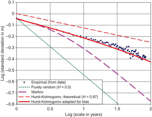
Figure 10 illustrates the empirical climacogram of the Nilometer time series for time scales 1 to 84 (years), as estimated from the time series , , . It also provides comparison of the empirical climacogram with those of a purely random process, a Markov process and an HK process fitted to empirical data. The slope of the empirical climacogram is clearly different from –0.5, i.e. that corresponding to a purely random process and a Markov process, and is consistent with the HK behaviour with H = 0.87.

Fig. 10 Climacogram of the Nilometer data and fitted theoretical climacograms of white noise (purely random process, equation (4)), a Markov process (equation (7)) and a HK process (equation (5)). For white noise the statistical bias is zero, for the Markov process it is negligible, while for the HK process it is large, and, therefore, a “model minus bias” line is also plotted; the bias is calculated based on a closed relationship in Koutsoyiannis (2003).

Essentially, the Hurst-Kolmogorov behaviour manifests that long-term changes are much more frequent and intense than is commonly perceived and, simultaneously, that the future states are much more uncertain and unpredictable on long time horizons (because the standard deviation is larger) than implied by pure randomness. Unfortunately, in the literature the high value of H has typically been interpreted as long-term or infinite memory. Despite being very common (e.g. Beran 1994), this is a bad and incorrect interpretation because it has several problems, i.e. (a) the metaphoric, typically unstated and undefined use of the term memory, perhaps as a synonym of autocorrelation, (b) the implication that the autocorrelation is the cause of the behaviour, while it is a consequence, and (c) the connotation of a passive and inertial mechanism related to memory, while the actual mechanism behind the HK behaviour should be active in order to produce long-term change. The first to criticize the memory interpretation was Klemeš (1974). The interpretation supported here is that a high H value indicates enhanced multi-scale change rather than memory. Furthermore, as will be seen below, H is a measure of entropy production, which is closely related to change.

The turbulent velocity time series shown in Fig. 7(a) contains a much larger number of data points (25 000) and allows the construction of a very detailed climacogram, albeit on very fine time scales (1.2 ms to 3 s). The climacogram is shown in Fig. 11 and is more complex than that of Fig. 10, as the slope is not constant for all time scales. Clearly the slope is much milder than –0.5 everywhere, which indicates that the turbulence process is far from purely random or Markovian. If we fit a HK model for scales of 30 ms to 3 s (a range extending over two orders of magnitude) this will give H = 0.77 (slope –0.23), which indicates strong HK behaviour. This value can be regarded as an asymptotic H for large scales, although even higher H would emerge if we restricted the fitting domain (leaving out the smallest scales). However, for small time scales, there appears a smoothing effect, i.e. decrease of variance with respect to the HK process, which could be thought of as the result of the fluid’s viscosity. A physical mechanism acting at very small scales and producing smoothing seems physically justified, as, without it, the variance would tend to infinity as k → 0 (see equation (6)) and this does not seem physically plausible.

Fig. 11 Climacogram of the turbulent flow velocity time series shown in Fig. 7(a) and fitted theoretical climacograms of white noise (purely random process, equation (4)), an HK process (equation (5)) and an HK process with low-scale smoothing (HKS; equation (8)). The HK process was fitted for scales >30 ms.

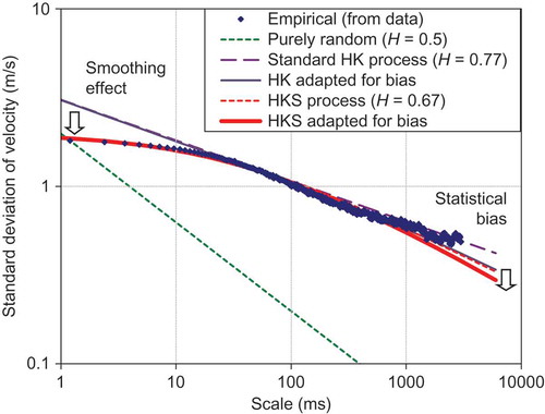
A simple modification of (6) in order to give a finite variance as k → 0, while retaining the HK properties for large scales, leads to (Koutsoyiannis 2013):

(8)

where a is a specified characteristic scale (not any scale as in (6)) and σ(a) is the process standard deviation at scale a. Apparently, the standard deviation at scale k → 0 is  σ(a), rather than infinite, as in the standard HK model, while for large scales equation (8) becomes indistinguishable from equation (6); therefore, we call the process defined by (8) the Hurst-Kolmogorov process with (low-scale) smoothing (HKS).

The process defined by equation (8) belongs to a family of processes that separate fractal dimension and the Hurst effect (Gneiting and Schlather 2004). It can be shown that the power spectrum of this process has two characteristic asymptotic slopes, 1 – 2H at low frequencies (large time scales) and –3 + 2H at high frequencies (small time scales). Therefore, if H = 2/3, then the slope at the high frequencies is –5/3, thus corresponding to the well-known “Kolmogorov’s 2/3 (or 5/3) Law” (Kolmogorov 1941, see also Shiryaev 1999). The HKS law (equation (8)) with fixed H = 2/3 is also plotted in Fig. 11 and seems consistent with turbulence measurements over the entire range of scales, although it overestimates the slope at very large scales (the slope of the empirical series is milder, corresponding to a higher H). A more detailed and more accurate model for these data has been studied (Koutsoyiannis 2012, Dimitriadis and Koutsoyiannis, in preparation), but is out of the scope of this paper; even in the detailed model, the essence remains that the climacogram slope for large scales verifies the Hurst-Kolmogorov behaviour.

CHANGE SEEN IN PROXY DATA

The time series of turbulent flow and of the Nile water level give us an idea of enhanced change and enhanced uncertainty as the time scale becomes larger. There are many more long instrumental hydroclimatic time series in which the HK behaviour has been verified. The Nile River basin offers some additional examples. Thus, high H values, close to those of the Nilometer minimum water levels, are estimated from the Nilometer record of maximum levels (Koutsoyiannis and Georgakakos 2006) and from the contemporary, 131-year-long flow record of the Nile flows at Aswan (Koutsoyiannis et al. 2008). Another example is offered by the water-level change of Lake Victoria, the largest tropical lake on Earth (68 800 km²) and the headwater of the White Nile (the western main branch of the Nile). The contemporary record of water level covers a period of more than a century (Sutcliffe and Petersen 2007) and indicates huge changes (Fig. 12(a)).

Fig. 12 (a) Contemporary record of the water level of Lake Victoria (from Sutcliffe and Petersen 2007). (b) Reconstruction of water level for past millennia from sediment cores (adapted from Stager et al. 2011).

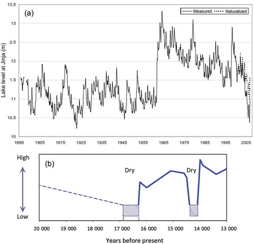
Unfortunately, however, instrumental records are too short to provide information on the entire range of changes that occurred throughout the millennia. It is therefore useful to enrol proxy data of different types, which, despite not being accurate, give some qualitative information of changes. For Lake Victoria, Stager et al. (2011) recently provided a reconstruction of its water level for past millennia using sediment cores. The study suggests that, strikingly, the lake was even dried up for several centuries at about 14 000 and 16 000 years before present (Fig. 12(b)).

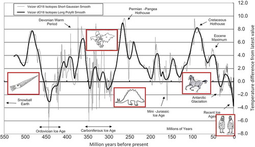
Obviously, all these examples reflect changes of the climate on Earth, whose history has been imprinted in several proxies. The longest palaeoclimate temperature reconstruction, which goes back more than half a billion years, was presented by Veizer et al. (2000) based on the ¹⁸O isotope in sediments, and the graph in Fig. 13 shows that change has occurred throughout time and at all time scales. As we can observe, today we are living in an interglacial period of an ice age. In the past, there were other ice ages, also known as icehouse periods, where glacial and interglacial periods alternated, as well as ages with higher temperatures, free of ice. Little is known about the causes of these changes, although there are strong links with Earth’s periodic orbital changes, the so-called Milankovitch cycles. Evidently, there are links with other aperiodic phenomena as the climate has co-evolved with tectonics (the motion of continents) and life on Earth.

Fig. 13 Palaeoclimate temperature reconstruction (adapted from Veizer et al. 2000; courtesy of Yannis Markonis). The graph also shows some landmarks providing links of the co-evolution of climate with tectonics (Pangaea) and life on Earth.

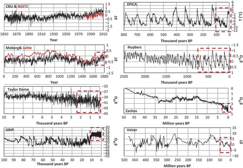
In a recent study, Markonis and Koutsoyiannis (2013) analysed 10 data series related to the evolution of the climate, specifically temperature, on Earth, starting from the most modern satellite-based temperature record, with a length of 32 years, and ending with the Veizer data series discussed above, covering about half a billion years. The different data series are plotted in Fig. 14 and their sources are provided in Table 1.

Table 1 Time series of global temperature based on instrumental and proxy data (for more details, see Markonis and Koutsoyiannis 2013)

Abbreviation	Reference	Type of data (unit)	Length (years)	Resolution (years)
NSSTC	http://www.nsstc.uah.edu	Satellite (°C)	32	1/12
CRU	Brohan et al. (2006)	Instrumental (°C)	161	1/12
Moberg	Moberg et al. (2005)	Multi-proxy (°C)	2 × 10^3	1
Lohle	Lohle (2007)	Multi-proxy (°C)	2 × 10^3	30*
Taylor	Steig et al. (2000)	Single-proxy ice core (δ^18O)	10 × 10^3	100
GRIP	Dansgaard et al. (1993)	Single-proxy ice core (δ^18O)	100 × 10^3	100
EPICA	Jouzel et al. (2007)	Single-proxy ice core (°C)	800 × 10^3	500
Huybers	Huybers (2007)	Multi-proxy sediment (δ^18O)	2.6 × 10^6	10^3
Zachos	Zachos et al. (2001)	Multi-proxy sediment (δ^18O)	60 × 10^6	50 × 10^3
Veizer	Veizer et al. (2000)	Multi-proxy sediment (°C)	480 × 10^6	500 × 10^3

Note: *Scales of 1 to 30 years were not included because the series is smoothed by Lohle (2007) at the 30-year scale.

Fig. 14 Global temperature series of instrumental data and reconstructions, described in Table 1, at different time scales, going back to about 500 million years before present (BP). The dashed rectangles provide the links of the time period of each time series with the one before it (adapted from Markonis and Koutsoyiannis 2013).

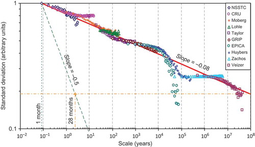
Now, if we construct the climacograms of the 10 time series and superimpose them after appropriate translation of the logarithm of standard deviation, but without modifying the slopes (see details of the methodology in Markonis and Koutsoyiannis 2013), we obtain the impressive overview of Fig. 15 for time scales spanning almost nine orders of magnitude—from 1 month to 50 million years. First, we observe in this big picture that the real-climate climacogram departs spectacularly from that of pure randomness. Second, the real climate is approximately consistent with an HK model with a Hurst coefficient of at least 0.92. (Note that statistical bias was not considered in estimating the slope –0.08 and therefore the value H = 0.92 can be regarded as a lower bound of the Hurst coefficient.) Third, there is a clear deviation of the simple scaling HK law for scales of 10–100 thousand years, exactly as expected due to the Milankovitch cycles acting at these time scales. Overall, the actual climatic variability at the scale of 100 million years equals that of about 2.5 years of a purely random climate! This dramatic effect should make us understand the inappropriateness of classical statistical thinking for climate. It should also help us understand what enhanced change and enhanced unpredictability are.

Fig. 15 Combined climacogram of the 10 temperature observation series and proxies. The solid straight line with slope –0.08 was fitted to the empirical climacogram, while the dashed line with slope –0.5 represents the climacogram of a purely random process. The horizontal dashed-dotted line represents the actual climatic variability at 100 million years, while the vertical dashed-dotted line at 28 months represents the scale corresponding to the 100-million-year variability if climate was purely random (classical statistics approach). For explanation about the groups of points departing from the solid straight line see text (from Markonis and Koutsoyiannis 2013).

Some imperfections observed in the matching of the climacograms of the different time series of Fig. 15 have been explained as the result of data uncertainties (both in sampling and aging) combined with the bias and enhanced uncertainty, which are implied by the long-term persistence in statistical estimation (Koutsoyiannis 2003, 2011b). Specifically, in some series, the right part of a climacogram is too flat (e.g. in Zachos and CRU time series). The reason for a flat right part is related to the fact that the entire time series length is located on a branch of the process with a monotonic trend (Fig. 14). When a longer time series is viewed (Veizer for Zachos, Moberg and Lohle for CRU), which shows that the monotonic trend is in fact part of a longer fluctuation, the flat climacogram problem is remedied. Another imperfection of Fig. 15 is related to the Huybers and EPICA climacograms, both of which have leftmost and rightmost parts with slopes milder and steeper, respectively, than the general slope. Particularly in the EPICA case, the rightmost part has a slope steeper than –0.5, which could be interpreted as indicating anti-persistence. However, as shown by Markonis and Koutsoyiannis (2013), this behaviour is fully explained by the combined effect of statistical bias and the influence of the orbital forcing.

FROM GEOPHYSICAL TO COSMOLOGICAL AND NON-MATERIAL PROCESSES

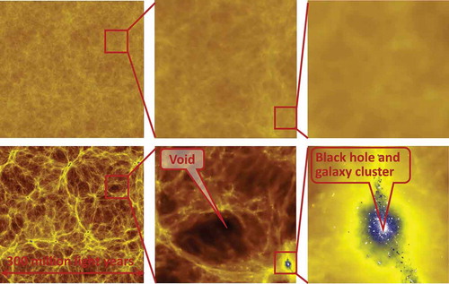
The presence of the HK behaviour is not limited to hydrology and climate. Further illustration of the clustering effect in geophysical processes is provided by Fig. 16, which shows that mega-earthquakes cluster in time, as do low seismicity periods. That is, the HK behaviour seems to be universal and, therefore, we should find it in the big picture of the universe itself. Indeed, the snapshots of Fig. 17 taken from videos depicting cosmological simulations indicate how the universe evolved from the initial uniform ‘soup’ to clustered structures, where the clusters are either voids or stars, galaxies and black holes. Uniformity (upper row of Fig. 17, corresponding to an early stage of the universe) is associated with maximum uncertainty at small scales, while clustering (lower row of Fig. 17, corresponding to a mature stage of the universe) reflects enhanced uncertainty at large scales.

Fig. 16 Cumulative seismic moment estimated for shallow earthquakes (depth ≤100 km and magnitude ≥7) (adapted from Ammon, http://www.iris.edu/news/events/japan2011/, who modified an earlier graph from Ammon et al. 2010). Dashed lines correspond to a constant moment rate 0.03 × 10²³ Nm/year for the indicated periods; moment magnitude values assumed for the largest earthquakes are 9.0 for Kamchatka 1952, 9.5 for Chile 1960, 9.2 for Alaska 1964, 9.15 for Sumatra 2004 and 9.05 for Japan 2011.

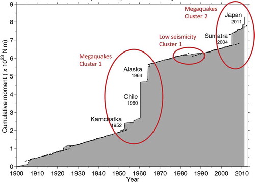
Fig. 17 Images from cosmological simulations of the growth of the universe, black holes and galaxies (snapshots from videos of cosmological simulations, timemachine.gigapan.org/wiki/Early_Universe; Di Matteo et al. 2008). Upper row: 200 million years after the Big Bang; lower row: 7 billion years later.

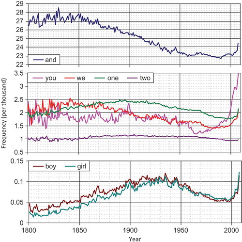
Moreover, the HK behaviour is a characteristic not only of the physical universe, but also of mental universes constructed by humans. Returning to the counts of words and phrases in books which we examined earlier, it is interesting to now inspect simple and unsophisticated words. Figure 18 depicts the evolution through the last couple of centuries of the use of very neutral and ingenuous words such as “and”, “you”, “we”, “one”, “two”, “boy”, “girl”. One might expect that the frequency of using these words should be static, not subject to change. But the reality is impressively different, as shown in these graphs. Their use is subject to spectacular change through the years.

Fig. 18 Evolution of the frequency per year of the indicated words of everyday language, as found in several million books digitized by Google covering the period from the beginning of the 19th century to present (the data are from 360 billion words contained in 3.3 million books published after 1800).

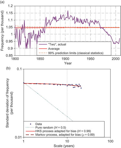
Most neutral and less changing seems to be the word “two”. However, a close-up on its time series, shown in Fig. 19(a), again reveals change different from pure randomness. The purely random approach is a spectacular failure, as indicated by the fact that almost all points of the time series lie outside of the 99% prediction limits calculated by classical statistics. The climacogram (Fig. 19(b)) indicates that the change is consistent with HK behaviour, with a Hurst coefficient very close to 1. Even a Markov (AR(1)) model with high autocorrelation can match this climacogram. In fact, the two models plotted in the figure, HKS and Markov, are indistinguishable in this case because the available record is too short for such high autocorrelation.

Fig. 19 (a) Close-up from Fig. 18 for the time series of the frequency of the word “two” and (b) its climacogram.

SEEKING EXPLANATION OF LONG-TERM CHANGE: MAXIMUM ENTROPY

Is there a physical explanation of this universal behaviour? Undoubtedly this question should have a positive answer. As proposed elsewhere (Koutsoyiannis 2011a), the answer should rely on the principle of maximum entropy, which is important both in physics (cf. the second law of thermodynamics) and in probability theory. Entropy is none other than a measure of uncertainty and its maximization means maximization of uncertainty. The modern formal definition of entropy is very economic as it only needs the concept of a random variable. The entropy of a continuous random variable x is a dimensionless quantity defined as (adapted from Papoulis 1991):

(9)

where f(x) is the probability density function of x, with ; l(x) is a Lebesgue density (numerically equal to 1 with dimensions the same as in f(x)); and E[ ] denotes expectation.

When temporal evolution matters, the quantity that we may seek to extremize is entropy production, a time derivative of entropy, rather than the entropy itself. Starting from a stationary stochastic process x(t) in continuous time t, first we define the cumulative (nonstationary) process as z and then we define the entropy production as the derivative of [z] with respect to time, i.e. , where the dimensions of are T⁻¹. To avoid some infinities emerging with and also construct a dimensionless entropy production metric, Koutsoyiannis (2011a) introduced the entropy production in logarithmic time (EPLT):

(10)

Observing that, for any specified time t and any two processes z₁(t) and z₂(t), an inequality relationship between entropy productions, such as also holds true for EPLTs, e.g. ϕ[z₁(t)] < ϕ[z₂(t)], the extremization of entropy production can be replaced by the extremization of EPLT. Koutsoyiannis (2011a) demonstrated that the HK process is derived by extremization of EPLT performed at asymptotic times (zero or infinity) and has a constant EPLT, independent of time. The constraints used in the extremization are elementary, namely the preservation of the mean, variance and lag-1 autocovariance at the observation time step, and an inequality relationship between conditional and unconditional entropy production, which is necessary to enable physical consistency. An impressive side-product of this study is that it gave the Hurst coefficient a clear physical meaning: it is the entropy production in logarithmic time, for time tending to infinity. A graphical illustration is provided in Fig. 20 for a positively autocorrelated process. It is seen that a Markov process maximizes EPLT as time tends to zero, but it gives the lowest possible EPLT value, 0.5, for large times. On the opposite side lies the HK process, which minimizes EPLT as time tends to zero and maximizes it for time tending to infinity, despite keeping a constant value throughout (EPLT = H = 0.92 in the example plotted in the figure). In other words, the enhanced change and enhanced uncertainty or entropy in the long run should result in the process having HK behaviour.

Fig. 20 Entropy production in logarithmic time ϕ(t) ≡ ϕ[z(t)] vs time t in two entropy-production extremizing processes, a Markov and a HK process, for lag-1 autocorrelation ρ = 0.79.

CONCLUDING REMARKS

The world exists only in change and change occurs at all time scales. Humans are part of the changing Nature and can themselves trigger change—but (fortunately) they cannot take full control of change. Moreover, change is hardly predictable in deterministic terms and demands stochastic descriptions. The Hurst-Kolmogorov stochastic dynamics is the key to perceive multi-scale change and model the implied uncertainty and risk.

Hydrology has contributed greatly to discovering and modelling change. However, lately, following other geophysical disciplines, it has been affected by 19th-century myths of static or clockwork systems, deterministic predictability (cf. climate models) and elimination of uncertainty. A new change of perspective is thus needed in which change and uncertainty are essential parts (cf. Koutsoyiannis et al. 2009, Koutsoyiannis 2010, Montanari and Koutsoyiannis 2012). The new scientific initiative of the International Association of Hydrological Sciences (IAHS) for the coming decade 2013–2022, entitled “Panta Rhei—Everything Flows” (Montanari et al. 2013), is expected to contribute substantially to such a mandate.

Acknowledgements

The idea of a presentation with this title grew from an invitation by David Legates, Willie Soon and Sultan Hameed to contribute to the session they planned within the American Geophysical Union Fall Meeting 2009 (session U06; “Diverse Views from Galileo’s Window: Researching Factors and Processes of Climate Change in the Age of Anthropogenic CO₂”; abstract #H33E-0944; adsabs.harvard.edu/abs/ 2009AGUFM.H33E0944K), which never materialized. I am grateful to Pierre Hubert, former Secretary General of IAHS, for suggesting I give a plenary lecture on the topic “Hydrology and Change” at the IUGG XXV General Assembly, Melbourne, Australia (5 July 2011), as well as to the IAHS President Gordon Young for his support and to the then IUGG President Tom Beer for his approval. I also thank the Hydrological Sciences Journal Editor Zbigniew Kundzewicz, who encouraged me to write up this essay based on the plenary lecture, as well as the anonymous reviewers Salvatore Grimaldi and Alberto Montanari for their encouraging and constructive comments.

Notes

¹Heraclitus’s writings have not survived but fragments thereof have been related by other authors; this one is from Plato’s Cratylus, 339–340.

²“”; ibid., 401d.

³“”; ibid., 402a.

⁴“”; ibid., 402a.

⁵“ ”; Meteorologica, I.14, 353a 16.

⁶“”; ibid., 356b 26.

⁷“”; ibid., II.2, 355a 26.

⁸“” Heraclitus, Fragment 52.

⁹Albert Einstein in a letter to Max Born in 1926.

REFERENCES

- Ad Hoc Panel on Hydrology 1962. Scientific hydrology. Washington, DC: US Federal Council for Science and Technology.
- Ammon, C.J., Lay, T., and Simpson, D.W., 2010. Great earthquakes and global seismic networks. Seismological Research Letters, 81, 965–971, doi:10.1785/gssrl.81.6.965.
- Beran, J., 1994. Statistics for long-memory processes. New York: Chapman and Hall.
- Brohan, P., et al., 2006. Uncertainty estimates in regional and global observed temperature changes: a new dataset from 1850. Journal of Geophysical Research, doi:10.1029/2005JD006548.
- Christofides, A. and Koutsoyiannis, D., 2011. God and the arrogant species: contrasting nature’s intrinsic uncertainty with our climate simulating supercomputers. In: 104th Annual conference & exhibition [online]. Orlando, FL: Air & Waste Management Association. Available from: http://itia.ntua.gr/1153/ [Accessed 6 May 2013].
- Dansgaard, W., et al., 1993. Evidence for general instability in past climate from a 250-kyr ice-core record. Nature, 364, 218–220.
- Di Matteo, T., et al., 2008. Direct cosmological simulations of the growth of black holes and galaxies. The Astrophysical Journal, 676 (1), 33–53.
- Gneiting, T. and Schlather, M., 2004. Stochastic models that separate fractal dimension and the Hurst effect. Society for Industrial and Applied Mathematics Review, 46 (2), 269–282.
- Hurst, H.E., 1951. Long term storage capacities of reservoirs. Transactions of the American Society of Civil Engineers, 116, 776–808.
- Huybers, P., 2007. Glacial variability over the last two million years: an extended depth derived age model, continuous obliquity pacing, and the Pleistocene progression. Quaternary Science Reviews, 26 (1–2), 37–55.
- Jouzel, J., et al., 2007. EPICA Dome C ice core 800KYr deuterium data and temperature estimates. Boulder, CO: IGBP PAGES/World Data Center for Paleoclimatology, 2007-091 NOAA/NCDC Paleoclimatology Program.
- Kang, H.S., Chester, S., and Meneveau, C., 2003. Decaying turbulence in an active-grid-generated flow and comparisons with large-eddy simulation. Journal of Fluid Mechanics, 480, 129–160.
- Klemeš, V., 1974. The Hurst phenomenon: a puzzle? Water Resources Research, 10 (4), 675–688.
- Kolmogorov, A.N., 1940. Wiener spirals and some other interesting curves in a Hilbert space. Dokl. Akad. Nauk SSSR, 26, 115–118. English translation in: V.M. Tikhomirov, ed., 1991. Selected works of A.N. Kolmogorov, Volume I: Mathematics and mechanics, 324–326. Berlin: Springer.
- Kolmogorov, A.N., 1941. Dissipation of energy in isotropic turbulence, Dokl. Akad. Nauk SSSR, 32 (1), 19–21 English translation in: V.M. Tikhomirov, ed., 1991. Selected works of A.N. Kolmogorov: Volume I: Mathematics and mechanics, 303–307. Berlin: Springer.
- Koutsoyiannis, D., 2002. The Hurst phenomenon and fractional Gaussian noise made easy. Hydrological Sciences Journal, 47 (4), 573–595.
- Koutsoyiannis, D., 2003. Climate change, the Hurst phenomenon, and hydrological statistics. Hydrological Sciences Journal, 48 (1), 3–24.
- Koutsoyiannis, D., 2010. HESS Opinions “A random walk on water”. Hydrology and Earth System Sciences, 14, 585–601.
- Koutsoyiannis, D., 2011a. Hurst-Kolmogorov dynamics as a result of extremal entropy production. Physica A: Statistical Mechanics and its Applications, 390 (8), 1424–1432.
- Koutsoyiannis, D., 2011b. Hurst-Kolmogorov dynamics and uncertainty. Journal of the American Water Resources Association, 47 (3), 481–495.
- Koutsoyiannis, D., 2012. Reconciling hydrology with engineering. In: IDRA 2012—XXXIII Conference of hydraulics and hydraulic engineering [online], Brescia. Available from: http://itia.ntua.gr/1235/ [Accessed 6 May 2013].
- Koutsoyiannis, D., 2013. Encolpion of stochastics: fundamentals of stochastic processes [online]. Athens: National Technical University of Athens. Available from: http://itia.ntua.gr/1317/ [Accessed 6 May 2013].
- Koutsoyiannis, D. and Georgakakos, A., 2006. Lessons from the long flow records of the Nile: determinism vs indeterminism and maximum entropy. In: 20 Years of nonlinear dynamics in geosciences [online], Rhodes. Available from: http://itia.ntua.gr/841/ [Accessed 6 May 2013].
- Koutsoyiannis, D. and Langousis, A., 2011, Precipitation. In: P. Wilderer and S. Uhlenbrook, eds. Treatise on water science. Oxford: Academic Press, 2, 27–78.
- Koutsoyiannis, D., Mamassis, N., and Tegos, A., 2007. Logical and illogical exegeses of hydrometeorological phenomena in ancient Greece. Water Science and Technology: Water Supply, 7 (1), 13–22.
- Koutsoyiannis, D. and Montanari, A., 2007. Statistical analysis of hydroclimatic time series: uncertainty and insights. Water Resources Research, 43 (5), W05429, doi:10.1029/2006WR005592.
- Koutsoyiannis, D., Yao, H., and Georgakakos, A., 2008. Medium-range flow prediction for the Nile: a comparison of stochastic and deterministic methods. Hydrological Sciences Journal, 53 (1), 142–164.
- Koutsoyiannis, D., et al., 2009. Climate, hydrology, energy, water: recognizing uncertainty and seeking sustainability. Hydrology and Earth System Sciences, 13, 247–257.
- Lohle, C., 2007. A 2000-year global temperature reconstruction based on non-treering proxies. Energy and Environment, 18 (7–8), 1049–1058.
- Mandelbrot, B.B. and van Ness, J.W., 1968. Fractional Brownian motion, fractional noises and applications. SIAM Review, 10, 422–437.
- Markonis, Y. and Koutsoyiannis, D., 2013. Climatic variability over time scales spanning nine orders of magnitude: Connecting Milankovitch cycles with Hurst-Kolmogorov dynamics. Surveys in Geophysics, 34 (2), 181–207.
- Michel, J.-B., et al., 2011. Quantitative analysis of culture using millions of digitized books. Science, 331 (6014), 176–182.
- Moberg, A., et al., 2005. Highly variable Northern Hemisphere temperatures reconstructed from low- and high-resolution proxy data. Nature, 433 (7026), 613–617.
- Montanari, A. and Koutsoyiannis, D. 2012. A blueprint for process-based modeling of uncertain hydrological systems. Water Resources Research, 48, W09555, doi:10.1029/2011WR011412.
- Montanari, A., et al., 2013. “Panta Rhei—Everything Flows”: Change in hydrology and society—The IAHS Scientific Decade 2013–2022. Hydrological Sciences Journal, 58 (6 ), doi:10.1080/02626667.2013.809088.
- Papoulis, A., 1991. Probability, random variables, and stochastic processes. 3rd ed. New York: McGraw-Hill.
- Shiryaev, A.N., 1999. Kolmogorov and the Turbulence. Centre for Mathematical Physics and Stochastics, University of Aarhus Available from http://webdoc.sub.gwdg.de/ebook/e/2002/maphysto/cgi-bin/w3-msql/publications/genericpublication.html@publ=100.htm
- Stager, J.C., et al., 2011. Catastrophic drought in the Afro-Asian monsoon region during Heinrich event. Science, doi:10.1126/science.1198322.
- Steig, E.J., et al., 2000. Wisconsinan and Holocene climate history from an ice core at Taylor Dome, Western Ross Embayment, Antarctica. Geografiska Annaler: Series A, Physical Geography 82 (2–3), 213–235.
- Sutcliffe, J.V. and Petersen, G., 2007. Lake Victoria: derivation of a corrected natural water level series. Hydrological Sciences Journal, 52 (6), 1316–1321.
- Toussoun, O., 1925. Mémoire sur l’histoire du Nil. Mémoire de l’Institut d’Egypte, 18, 366–404.
- UNESCO (United Nations Educational, Scientific and Cultural Organization), 1963. Preparatory meeting on the long-term programme of research in scientific hydrology. Paris: UNESCO. Available from: http://unesdoc.unesco.org/images/0001/000173/017325EB.pdf
- UNESCO (United Nations Educational, Scientific and Cultural Organization), 1964. International Hydrological Decade. Intergovernmental Meeting of Experts. Paris: UNESCO. Available from: http://unesdoc.unesco.org/images/0001/000170/017099EB.pdf
- Veizer, J., et al., 2000. 87Sr/86Sr, d13C and d18O evolution of Phanerozoic seawater. Chemical Geology, 161, 59–88.
- Zachos, J., et al., 2001. Trends, rhythms, and aberrations in global climate 65 Ma to present. Science, 292 (5517), 686–693.