Estimation of the temporal autocorrelation structure by the collocation technique with an emphasis on soil moisture studies

Abstract

The collocation technique has become a popular tool in oceanography and hydrology for estimating the error variances of different data sources such as in situ sensors, models and remote sensing products. It is also possible to determine calibration constants, for example to account for an off-set between the data sources. So far, the temporal autocorrelation structure of the errors has not been studied, although it is known that it has detrimental effects on the results of the collocation technique, in particular when calibration constants are also determined. This paper shows how the (triple) collocation estimators can be adapted to retrieve the autocovariance functions; the statistical properties as well as the structural deficencies are described. The coupling between the autocorrelation of the error and the estimation of calibration constants is studied in detail, due to its importance for analysing temporal changes. In soil moisture applications, such time variations can be induced, for example, by seasonal changes in the vegetation cover, which affect both models and remote sensing products. The limitations of the proposed technique associated with these considerations are analysed using remote sensing and in situ soil moisture data. The variability of the inter-sensor calibration and the autocovariance are shown to be closely related to temporal patterns of the data.

Editor D. Koutsoyiannis

Citation Zwieback, S., Dorigo, W., and Wagner, W., 2013. Estimation of the temporal autocorrelation structure by the collocation technique with an emphasis on soil moisture studies. Hydrological Sciences Journal, 58 (8), 1729–1747.

Résumé

La technique de collocation est devenue un outil courant en océanographie et en hydrologie pour estimer les variances d’erreur de différentes sources de données telles que les capteurs in situ, les modèles et les produits issus de la télédétection. Elle permet également de déterminer les constantes d’étalonnage, par exemple pour tenir compte des différences selon la source des données. Jusqu’à présent, la structure d’autocorrélation temporelle des erreurs n’a pas été étudiée, mais on sait qu’elle a des effets néfastes sur les résultats de la technique de collocation, en particulier lorsque cette dernière sert à déterminer les constantes d’étalonnage. Dans cet article, on montre comment les estimateurs de collocation peuvent être adaptés pour atteindre les fonctions d’autocovariance. Les propriétés statistiques ainsi que les défauts structurels sont décrits. Le couplage entre l’autocorrélation de l’erreur et l’estimation des constantes d’étalonnage a été étudié en détail, en raison de son importance pour l’analyse des changements temporels. Dans les applications concernant l’humidité du sol, ces variations temporelles peuvent être induites, par exemple, par les variations saisonnières de la couverture végétale, qui affectent à la fois les modèles et les produits dérivés de la télédétection. Prenant en compte les limites de la technique proposée ainsi que les considérations précédentes nous avons utilisé des données d’humidité du sol mesurées in situ et d’autres issues de la télédétection. On a pu montrer que la variabilité de l’étalonnage entre les capteurs et l’autocovariance sont étroitement liées aux tendances temporelles des données.

Key words:

• soil moisture
• validation
• time series analysis
• remote sensing
• error analysis

Mots clefs:

• humidité du sol
• validation
• analyse des séries chronologiques
• télédétection
• analyse d’erreur

1 INTRODUCTION

The collocation technique is commonly applied to the estimation of the error of remote sensing products and model data. It is particularly popular in oceanography (Stoffelen 1998, O’Carroll et al. 2008, Winterfeldt et al. 2010), but also in soil moisture research (e.g. Scipal et al. 2008, Dorigo et al. 2010, Hain et al. 2011, Loew and Schlenz 2011, Parrens et al. 2012). The most common instance by far is the triple collocation method, which can retrieve the error variance of three data sets, each of which measures the same parameter. As the data of different models and measurements often differ in their mean and dynamic range, it is commonplace to estimate inter-sensor calibration constants to account for these discrepancies; the collocation technique can be applied to such data in modified form (Zwieback et al. 2012a).

Previous studies have always looked at time series: for instance the unknown soil moisture at time t, x^t, is recorded by various data sources . The application of the collocation technique to time series data raises two important questions: (i) Is the error structure homogeneous in time?; (ii) Are the errors at different epochs correlated? Issue (i) can sometimes be addressed by reducing the temporal extent until the assumption of homogeneity is permissible. Question (ii) is potentially even more difficult.¹ In most previous studies, these temporal variations were neglected altogether, even though the analysis of trends or temporal fluctuations is of considerable scientific interest.

As shown in Zwieback et al. (2012a), the presence of autocorrelation has the following impacts on the standard collocation estimators:

• Bias: when there are calibration constants to be estimated, the usual error variance (and covariance) become biased.

• Standard errors: the usual expressions for the standard errors cease to be valid; usually, the standard errors will be larger than indicated by these formulas.

• Calibration constants: the estimator of the additive constant α remains unbiased, but ceases to be the best unbiased linear estimator; the corresponding estimator of the error variance becomes biased. The issues with the estimation of the multiplicative constant β become exacerbated.

The bias is particularly pronounced when the number of samples is small, which, for example, is the case when temporal dynamics are to be investigated. The intuitive explanation for this bias is that when the data cover a temporal period of the order of the correlation length, the calibration constant can adapt to this, essentially providing an overfitting. In practice, it is important but also very difficult to define what part of the deviation is stochastic (thus described by the error term and possibly autocorrelated) and what part is systematic. In remote sensing of soil moisture, for example, both the bias and the stochastic errors are possibly functions of time, e.g. due to changing vegetation cover. A better understanding of the temporal variations can lead to improvements of models and remote sensing products, but is also beneficial for hydrological analyses, such as the spatial scaling of soil moisture (Loew and Schlenz 2011).

As previously mentioned, the standard collocation technique is subject to deleterious influences in the presence of autocorrelation. However, by a slight modification the collocation technique can also be applied to the estimation of the autocovariance structure of the measurement error, thus potentially allowing a more comprehensive characterization. The autocorrelation is particularly relevant for uncertainty analysis in forecasting and complex modelling scenarios (e.g. Shiklomanov et al. 2006, Habib et al. 2008, Hossain and Huffman 2008). In Section 2 we introduce the “nuts and bolts” of the standard collocation method and the notation. Subsequently (Section 3), the collocation estimators are adapted to the determination of the autocovariance structure. Analogously to the usual retrieval of the error variance, only certain parts of the autocovariance structure can be estimated by the collocation technique, i.e. certain components are not resolvable; Section 4 shows how many degrees of freedom there are and exactly what parts can be retrieved. The estimator for the autocovariance is analysed in Section 5; in particular, the estimator variance is given for the simplest possible case. These estimators are applied to simulated data in Section 6, thus permitting the validation of the analytical results. Two small case studies serve to illustrate the properties and issues mentioned above: firstly, in Section 7, the temporal variability of the calibration constants is shown for an area in Spain, comparing a remote sensing product, a model and the measured in situ soil moisture in a classical triple collocation study. Secondly, the structural limitations of the collocation technique are illustrated in a hypothetical scenario, in which we attempt to apply a statistical test to analyse temporal changes in the records of five in situ soil moisture probes (Section 8).

2 FUNDAMENTALS

In its simplest form the (triple) collocation technique assumes the following error structure (referred to as the basic model in Zwieback et al. 2012a):

(1)

where y_i represents the measurement by sensor i of the unknown quantity x and e_i is the random error. The error variance can be estimated by the standard collocation technique without making any assumptions about the parameter x if:

• there are three or more data sources,

• the measurements are unbiased, i.e. ,

• the errors are mutually uncorrelated, i.e. ,

In this case, the expected value of the estimator is the error variance of sensor i:

(2)

where the combination of the sensors can be conveniently summarized in the bracket notation . This example forms the heart of the triple collocation technique, as only three data sets are necessary to estimate all the error variances. The incorporation of additional sensors is possible, as is the relaxation of some of the above-mentioned assumptions; cf. Zwieback et al. (2012a) for a detailed analysis.

In previous studies it was often deemed necessary to estimate bias terms α between the data sets as these were off-set with respect to one another. In a similar vein, a multiplicative bias term β can be introduced to match the dynamic ranges of the data sets. This leads to a more general error model:

(3)

In this context, the parameters and are often referred to as calibration constants. The estimation of the error variances is then conducted in two steps. In the first one, the data are scaled to the sensor of reference (taken to be number 1) for which and :

(4)

i.e. a relationship of the kind of equation (1) is created with a modified error term . In reality, of course, and , are not known, but have to be estimated from the data as well: , ; the operation of equation (4) is then performed with these estimates. The second step consists of the usual analysis based on the modified data of equation (4). If the calibration constants are estimated from the same data, the collocation estimators can be modified to account for this, cf. Zwieback et al. (2012a).

In the following we will mostly deal with time-discrete series: the number of the measurement (i.e. temporal reference) is denoted by a superscript, e.g. for the parameter value at time t. For certain operations it is convenient to think of all the errors or measurements at one epoch t as a (column) vector. This will be denoted by bold-italic notation, e.g. and the components by subscripts.

3 ESTIMATION OF THE AUTOCOVARIANCE MATRIX

3.1 Notation

The autocovariance matrix of lag (which indicates the time difference) is denoted by ; it is of size M × M and its elements are defined by (assuming bias-free errors):

(5)

i.e. . If the error structure is assumed to be homogeneous in time (weak or wide-sense stationarity of the errors), is not a function of time t.

We simply mention two important properties here:

3.1.1 Time reversal of τ

It follows directly from the definition that , and thus , if wide-sense stationarity holds.

3.1.2 Positive semi-definiteness

For any set of vectors of dimension M, has to hold as (see Reinsel 1997). It often proves more convenient to study the autocorrelation, which for a wide-sense stationary process is given by .

3.2 Sampling the autocovariance matrix

A simple adaptation of the collocation estimators makes them capable of retrieving the autocovariance structure:

(6)

where the second part follows from the error model, equation (1). Without loss of generality, will be assumed. Note that the quantity in equation (6) depends on t; however, this dependence disappears as soon as we form expectations—wide-sense stationarity will be assumed in the remainder:

(7)

In perfect analogy to the standard collocation technique, equation (7) essentially corresponds to a sampling of the autocovariance matrix.

4 STRUCTURAL LIMITATIONS

4.1 Estimators of the collocation kind

The quantity can be generalized in such a way that the difference in either parenthesis is replaced by a linear combination whose coefficients sum to 0. This we refer to as the most general estimator of the collocation kind. We express this as (the vectors of coefficients are referred to as a and b):

(8)

the second part of which follows if (and for general x only if) the coefficients and sum to 0. In what follows, all vectors refer to the standard basis and we will employ the standard inner product. Thus we can express equation (8) as:

(9)

This framework and notation will be useful in analysing what parts of are accessible by the sampling procedure of equation (7).

4.2 Change of basis

As mentioned above, the coefficients of the linear combinations a and b have to sum to 0. It is thus more natural to work in a different basis (), where the jth coefficient of in the standard basis is –1 if i = j, 1 if j = i + 1, and 0 otherwise. This allows us to express and and thus to rewrite equation (9) as:

(10)

The terms are instances of equation (6), i.e. there are only single differences between two measurements in either parenthesis in equation (8).

The vector v whose coefficients are all 1 in the standard basis is orthogonal to all and together they form a basis for the complete vector space.

For the subsequent analysis, we note that equation (9) can also be expressed as:

(11)

which we will take to be the inner product between and .

4.3 Resolvable structure

We will now address the following question: Which parts of the autocorrelation structure can be estimated by the collocation technique, i.e. by estimators of the type of equation (8)? It will be most convenient to tackle the issue using the notation established in equation (11); will be considered fixed and greater than 1. Due to the linearity in the outer product , we only have to analyse the inner products between and in equation (10).

As the form a basis for the complete vector space together with v, we can express as follows:

(12)

There are coefficients , each of and and : the total is . In fact equation (12) is a special case, as the corresponding matrix is of rank 1, but we will look at general autocovariance matrices later.

As shown in the previous analyses, we can form estimators of the kind ; they correspond to inner products between and the observed quantity . The latter can be expanded in the form shown in equation (12). Due to linearity, we can look at the inner products between and the outer products of the basis vectors separately; in particular the following ones evaluate to 0:

• Base outer product : these vanish because because .

• Base outer product : due to , we have .

• Base outer product : for the same reason, we have .

This means that the coefficients corresponding to these base elements, i.e. , and cannot be retrieved by the collocation technique—they are invisible to all possible estimators. The can be found by solving a system of linear equations (which has a unique solution, as the are independent).

So far we have only looked at a single dyad of data . This was not a serious restriction, as the inner product is a linear operator. We can thus easily average over t, or form expectation values:

(13)

4.4 Summary

The previous analysis has shown that there are only degrees of freedom that can be resolved. The coefficients , and cannot be retrieved. There are three important points to note. First, the number of degrees of freedom is greater than in the “standard” collocation technique (i.e. when estimating the covariance matrix); the autocovariance matrix itself, however, has more degrees of freedom than the covariance matrix as it is not symmetric. Second, the base expansion of equation (12) is probably not particularly amenable to practical situations, where restrictions will often be of a different form, e.g. that certain elements of the autocovariance matrix are assumed to be 0. In such cases a more detailed analysis will be necessary to ensure that the matrix of the system of equations has full rank. Third, it might seem possible to extract further information by making use of the time reversal property stated in Section 3.1. However, the restriction of did not entail any loss of generality as:

(14)

Thus, apart from the change of temporal reference , this simply corresponds to a switch .

5 STATISTICAL PROPERTIES OF THE ESTIMATOR

5.1 Assumptions and bias

When the autocovariance matrix is expanded as described in equation (12), the coefficients , and cannot be determined by the collocation technique. In the simplest scenario imaginable, they can be assumed to vanish; alternatively, they could be known (or rather, postulated) beforehand.

Due to the linearity of both the inner product and the expectation operator equation (13), unbiasedness follows directly when solving the system of linear equations (provided the aforementioned assumption is valid). This can be illustrated with reference to the most prominent special case: the triple collocation technique (M = 3), where all the cross-autocovariances are assumed to vanish. This is an example of a case where the regularity of the system of equations is ensured by imposing different constraints than setting , and to 0. Let and ; then:

(15)

where the last line follows from our assumptions. Note that we did not even have to solve a system of equations by virtue of the assumptions and the choice of a and b.

In order to reduce the uncertainty, more data will be incorporated in general. Due to linearity, it follows that:

(16)

with N the number of epochs. In the triple collocation case the expected value is clearly . The analysis for the two remaining data sources is analogous.

5.2 Estimator variance

For any random variable X, the variance is given by:

(17)

Let us have a look at defined in equation (16)—in the notation of equation (6) this can also be denoted by . As it is unbiased given our assumptions, the second term in equation (17) is simply —the difficulty is the evaluation of :

(18)

i.e. it all boils down to evaluating 16 products of the form (with i, j, k and l being general indices):

(19)

This is quite a challenge. In order to derive a solution, we will concentrate on the simplest case possible and make the following additional assumptions:

1. the errors are assumed to follow an MA(1) process, i.e. , , ;

2. thus we only need to look at and ; and

3. the errors are assumed to follow a Gaussian Process, so that equation (19) can be evaluated by Isserlis’ theorem (equation (20); cf. Koopmans 1995):

   (20)

Due to assumptions (a) and (b), only a handful of combinations of and yield distinct values. Let us now analyse the case of in more detail. In this case all products are equivalent except for those with . If we imagine and to form a two-dimensional array, these are the cases we have to consider:

• Diagonal = t: There are clearly N such terms, each of them evaluated as—using equation (20) and :

• Sub-diagonal 1 = t + 1: There are N – 1 of these terms, each of them yielding:

• Super-diagonal = t –1: cf. sub-diagonal 1

• Sub-diagonal 2 = t + 2: There are N – 2 of these terms:

• Super-diagonal 2 = t – 2: cf. sub-diagonal 2

• Off diagonal |– t| > 2: There are of these:

The sum of these terms for each of the 16 products in equation (18) is most conveniently evaluated in a computer algebra system. After substitution into equation (17), we arrive at:

(21)

and similarly for :

(22)

These results exhibit the permutational symmetries expected from the solution. As expected, equation (22) collapses to the one obtained for the standard collocation method (see Zwieback et al. 2012a) if all autocovariances vanish.

5.2.1 Quadruple collocation case with one covariance

We will now briefly look at the estimation of cross-covariances. Let and the only non-vanishing cross-covariance for both and be , i.e. and both vanish unless , or , except for . Then it is easy to show that equation (16) is an unbiased estimator for and () when and . We will merely state the resulting estimator variances:

(23)

(24)

5.3 Inclusion of the additive calibration constant α

5.3.1 Mathematical treatment

In many practical cases there is a bias between the data sources; in this case, the basic error model (equation (1)) is not valid. Instead the so-called bias model applies:

(25)

This is a simplification of the affine model of equation (3), but the structure is sufficiently simple so that the properties are well known (Zwieback et al. 2012a).

As the collocation technique makes no assumptions about the unknown parameter x, one of the sensors is taken as reference, such that its bias is by definition 0; without loss of generality, we will denote this data source by the index 1. If there is no autocorrelation present, the estimator of equation (26) is the best, linear (in the difference) unbiased estimator of (Zwieback et al. 2012a). If, on the other hand, the errors are autocorrelated, this estimator is still unbiased, but ceases to be optimal with respect to the previously mentioned criterion. An optimal estimator could be designed if the error structure were known, but it generally is not. We will thus continue to estimate α with equation (26):

(26)

To study the influence of the estimated calibration constant on the estimated error covariance, we will look at a simple case: equation (16) with , and , i.e. the standard triple collocation scenario of Stoffelen (1998). The treatment could of course be made more general, but it would result in unwieldy and complicated expressions that would only provide limited insight and practical benefit. Following the same approach adopted in the standard collocation technique (Zwieback et al. 2012a), we have to adapt the estimator by subtracting the estimated calibration constants, which we indicate by a prime:

(27)

where the last line follows from the error model, equation (25) and the definition of and where is a normalization factor that has to be determined. Expanding equation (27) and taking the expected value:

(28)

If the noise is white, i.e. for , equation (28) simplifies tremendously—the summands are written in the same order as above:

(29)

from which we see that the choice ensures unbiasedness of the estimator. It turns out that also for different brackets, e.g. (cf. Zwieback et al. 2012a).

Our main interest, however, rests on those instances when the noise is not white. Equation (28) can, of course, be evaluated for any noise model such as MA or AR processes. However, it is more insightful to study the case of a general autocorrelation function, which exhibits positive correlations up to a characteristic lag , beyond which all correlations can be neglected. The first term of equation (28) is unaffected by these autocorrelations, and also the second and fourth term always cancel. In the third term there are four terms of the type:

(30)

where the term accounts for the edge effects, i.e. when and thus outside the sample. As N increases, the influence of these edge effects diminishes as O(τ₀/N), such that equation (30) simplifies to with . Letting , we finally obtain combination with the first line of equation (28):

(31)

Thus, if we use the usual normalization constant Z = N – 1, our estimates will be too small on average if  . This effect will become less pronounced as N increases. The intuitive explanation for this behaviour is that, for a period of the order of , the errors tend to be correlated; for example, they all tend to be positive during such a period. The can adapt to this and, consequently, the overall spread of the errors appears to be smaller than it really is. As increases (τ₀/N = 1), this power to adapt becomes increasingly weak; the correction factor in equation (31) approaches 1 as O(1/N). Note that for small the edge effects cannot be neglected and that this argument hinges on the the simplification .

5.3.2 Practicalities

It is important to emphasize that these difficulties arise from the simultaneous estimation of the calibration and error structure. They will not occur if α is known beforehand or, more likely, from different data, e.g. from a different year. In the latter scenario, one has to take care that there are no autocorrelations between different years—for example, this might occur due to the similar impact of vegetation on modelled or remotely sensed data during the same season for subsequent years—the expected value of the error should still be zero due to the calibration constants. A different (and more common) approach is the decomposition of the measurement into a long-term mean (climatology) and a deviation (anomaly) (e.g. Dorigo et al. 2010, Miraelles et al. 2012). The long-term mean, however, has to be estimated from the data: in the framework of the bias error model of equation (25), (where is the—unknown—mean value of x in a suitable time window, and the average error), such that the (estimated) anomaly . This is essentially the same as the usual way of normalization by subtraction of , apart from the fact that x is replaced by and that all sensors are treated equal, i.e. there is no reference. The presence of the average error introduces the same kinds of autocorrelations between different epochs as the procedure described above, and also carries over to different decompositions of the signal into climatology/anomaly such as those employed by Dorigo et al. (2010) or Parrens et al. (2012).

6 SIMULATION STUDY

We will look at the simple case analysed in the previous section: a triple collocation () study, where the errors are a realization of a zero-mean MA1 Gaussian process, the covariance matrices being as follows:

(32)

Note that all the off-diagonal vanish in either case, so that we can use the kind of estimators that are regularly employed for triple collocation studies (Scipal et al. 2008). According to the basic model in equation (1), we obtain the simulated measurements by adding the parameter to the simulated noise . As the parameter drops out of the results by virtue of the design of the collocation estimators, we could simply set it to 0 for all t. However, we will simulate it in the same way as in Zwieback et al. (2012a): the are drawn independently from a uniform distribution, with values ranging from 0 to 10, and subsequently smoothed with a boxcar filter of length 5.

An exemplary time series consisting of N = 60 values is shown in Fig. 1(a).

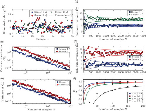
Fig. 1 Results of the simulation studies (see Section 6): (a) exemplary time series simulated using the procedure and parameters outlined; (b) convergence of the estimators for the variance equation (16): solid lines indicate ±2 SE range from equation (22); (c) convergence of the variance of the estimated variance: the markers indicate the sample variance obtained by running 50 simulations for each N; solid lines are from equation (20); (d) convergence of the estimators for the variance equation (16); solid lines indicate the ±2 SE range from equation (21); (e) convergence of the variance of the estimated variance: the markers indicate the sample variance obtained by running 50 simulations for each N; solid lines are from equation (21); and (f) comparison of the empirical normalization factor of equation (36) with the number of samples N; solid lines are from equation (36).

6.1 Estimation τ = 0

In Fig. 1(b) the convergence of the estimated variances as defined in equation (16) (with the appropriate choice of the vectors a, b) is shown as the number of samples N increases. The solid lines mark the range around the actual values, the standard errors SE being the square roots of the estimator variance, equation (22).

The standard errors diminish as O(N^−1/2) or, equivalently, the error variance as O(N⁻¹). This is emphasized by Fig. 1(c), where the theoretical values given by equation (22) are compared to simulated sample variances; these are obtained by simulating 50 time series for each N and computing the sample variance of the estimated values. Note that unlike for the standard collocation technique (no autocovariance), the variance is not exactly proportional to N⁻¹, although this is negligible for large N; the deviation from a straight line is not noticeable in Fig. 1(c).

6.2 Estimation τ = 1

Figure 1(d) shows the application of the estimator of equation (16) with to the experiments described in the previous section. The conclusions about the influence of the sample size on both the estimated value and the standard error are virtually identical to the case of : the standard error diminishes essentially as N^−1/2. The deviations are barely noticeable in Fig. 1(e), which is analogous to Fig. 1(c). The simulated results are in line with the theoretical formulae of Section 5.

6.3 Bias due to estimation of calibration constant α

The analysis in Section 5.3 revealed that the presence of autocorrelations will lead to biased estimates of the error variances and covariances if the calibration constant is estimated from the same data (using equation (25)). These autocorrelations will be positive in most studies, in which case the estimates will be too low. As the error structure is not known and cannot be resolved entirely due to the structural deficiencies of the collocation technique, the most pertinent issue is the behaviour of the bias as the number of samples increases. According to the analysis in Section 5.3, equation (31), the estimated variance will be wrong by a factor that approaches 1 as O(1/N).

This behaviour will be illustrated using simulated data with the number of sensors M = 3. The are drawn as before, but the simulated errors are drawn from a multivariate Gaussian AR(1) process according to:

(33)

where the is a Gaussian white noise process, the covariance matrix of which is taken to be the identity for simplicity. The autocovariance function of can be shown to evaluate to (Reinsel 1997):

(34)

where is the Kronecker delta.

For simplicity, only the estimation of will be studied, using the standard combination . Note that due to the lack of cross-correlation between the sensors for all , only the terms in equation (28) are non-zero. For fixed values of and N, the normalization constant can be estimated from the simulated data, as the error variance is known:

(35)

If there were no autocorrelation present (ρ = 0) the expected value of would be N – 1. In the presence of autocorrelation, an approximate expression can be found in equation (31), which for the noise process studied in this section is given by:

(36)

Figure 1(f) illustrates the convergence of to 1 for different values of and N. For each combination of and , 1500 independent estimates were drawn; the arithmetic mean of these values is plotted in the Fig. 1(f). The approximate expression from equation (36) is shown for comparison. Note that the approximation relies on the assumption of large N, so that the edge effects are negligible. For small N, equation (36) yields values which are too small, which is evident in the figure for ρ = 0.9.

7 CASE STUDY 1

7.1 Overview

The REMEDHUS network in central Spain (centre coordinates: 41.3° N, 5.4° W) provides the opportunity to estimate the error structure and calibration constants. The study area is part of the Duero basin and characterized by a semi-arid climate (average precipitation of 385 mm). The land cover is predominantly agricultural crops (in particular cereals). The years 2007–2009 are studied. The following soil moisture data sets are available:

• In situ: mean of all 22 sensors (impedance probes, 0–5 cm depth) of the REMEDHUS network (Dorigo et al. 2011, Sánchez et al. 2012).

• Advanced SCATterometer (ASCAT): soil moisture derived from scatterometer measurements, as described by Naeimi et al. (2009) (C-band radar, resolution: 50 km, rescaled to range [0,1], GP: 2147256).

• ECMWF Reanalysis (ERA) Interim: modelled soil moisture of global re-analysis data set ERA Interim (Dee et al. 2011) (top-most layer, resolution: 80 km, temporal resolution: 6 h, GP: 16069).

The temporal matching is obtained by linear interpolation to the ASCAT observation if the temporal difference is less than 6 h.

This case study is an extension of Zwieback et al. (2012b), where the temporal variability of the error and calibration constants was analysed using ERA Interim and ASCAT data and one in situ sensor. The analysis will now be extended to include the estimation of the autocorrelation and how this relates to the time-variant calibration. Note that it is the autocorrelation of the errors that is retrieved, not the autocorrelation of the soil moisture time series, as the triple collocation is by construction insensitive to the latter. For an analysis of this kind of autocorrelation, see e.g. Parlange et al. (1992) and Koster and Suarez (2001).

An overview of the data is given in Fig. 2(a). The ASCAT soil moisture represents the degree of saturation rather than volumetric soil moisture, which is the quantity represented by the other data sets. The in situ and ERA Interim data sets have to be calibrated with respect to each other as well; this is not uncommon for land surface models (Koster and Milly 1997, Entekhabi et al. 2010). A close look reveals that these differences vary with time and that this concerns both the off-set (bias) as well as the differences in the dynamic range. The temporal evolution also shows dissimilarities, e.g. the slow drying in July 2007.

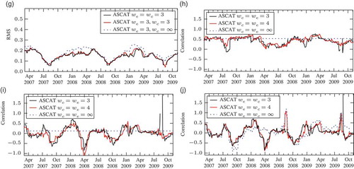
Fig. 2 Results of case study 1: calibration constants, RMS errors (square root of estimated variance) and autocorrelations. The window sizes w_c and w_e are expressed in months: (a) the soil moisture time series; (b) estimated α for ASCAT; (c) estimated β for ASCAT; (d) estimated RMS of ASCAT, w_c = w_e; (e) estimated RMS of ASCAT w_c  w_e; (f) estimated RMS of ASCAT, in ASCAT climatology, w_c = w_e; (g) estimated RMS of ASCAT, in ASCAT climatology, w_c  w_e; (h) autocorrelation of ASCAT errors, τ = 1 d; (i) autocorrelation of ASCAT errors, τ = 10 d, w_c = w_e; and (j) autocorrelation of ASCAT errors, τ = 10 d, w_c  w_e.

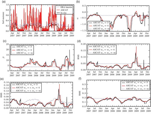
Fig. 2 (Continued)

7.2 Computations

As both the mean and the spread of the various data sets are different, the affine model of equation (3) is applied and the in situ data taken as reference (sensor 1). After estimation of and (Caires and Sterl 2003), the data are expressed in the climatology of the in situ probes, i.e. equation (3) is inverted:

(37)

The usual triple collocation estimators of Section 2 can then be applied. Note that the error variances of, for example, the ASCAT product is now expressed in terms of the in situ measurement rather than its own “units”. The conversion can be achieved by multiplying by () for the variance (root mean square (RMS) error). Similarly, the autocorrelation can be retrieved according to equation (16)—as the data samples are not regular in time, they are binned with a slot size of one day (see Rehfeld et al. 2011). As the focal point of this analysis is the study of the temporal variations and their connection to the autocorrelation, both the calibration constants and the error (autoco)variances are estimated in temporal windows: for a window of size , the estimation at time incorporates all measurements at times for which .

The temporal window for the estimation of the calibration constants is denoted by , the one for the estimation of the error variance by (both expressed in months for convenience). For the latter, the rescaling operation of equation (37) is done using the same calibrations constants for all observations in the window . In Zwieback et al. (2012b) this method (non-individual rescaling) was shown to lead to more stable results compared to other ways of conducting the rescaling.

7.3 Estimation of the calibration constants

The retrieved estimates of and (ASCAT) for different window sizes (expressed in months) are shown in Fig. 2(b) and (c), respectively. In particular —which matches the dynamic ranges—fluctuates: in winter (e.g. January 2009), it reaches very large values as the ASCAT data set makes use of its range, whereas the in situ data are limited to a small interval. As observed in Zwieback et al. (2012b), the estimation is not robust during summer, as both data sets are restricted to small intervals due to dryness and thus the variations are more strongly influenced by the noise. This sensitivity is related to the structure of the estimator (Zwieback et al. 2012b), cf. e.g. the outlier at the end of September 2009 for .

7.4 Estimation of error variances

The estimated error of ASCAT, expressed as the RMS error, is shown in Fig. 2(d) and (e). In the former, both the calibration and errors are estimated in the same window; but varies in the latter. The results are remarkably sensitive to this choice and also to the kind of rescaling (cf. Zwieback et al. 2012b). The outlier for in April 2009 is caused by the exceedingly small value of ; this is again due to the structure of the estimator, as explained in Zwieback et al. (2012b). The differences between window sizes of 3 or 4 months is, apart from several such deviations, small.

The time-invariant calibration constants () differ in particular during winter from those estimated in smaller windows. The impact of their temporal variability on the retrieved error is shown in Fig. 2(f); the temporal variation of the error (, ) is qualitatively different, in particular during winter. The time dependence of the calibration is also evident when the error is scaled back to the ASCAT climatology, i.e. multiplied by , as described in Section 7.2. This is illustrated in Fig. 2(f) and (g), where the dry season, during which tends to be small, is characterized by small RMS errors. The seasonal signal appears to be considerably stronger when the error is expressed in the ASCAT climatology, with low errors occuring during summer. This is the dry season and the vegetation cover is sparse compared to spring; note, however, that the seasonal patterns are very sensitive to the representation of the error (in ASCAT or in situ climatology) because the calibration constants change.

7.5 Estimation of error autocovariances

The autocorrelation (as defined in Section 3.1, with the theoretical values being replaced by estimates) of ASCAT (1-day separation), retrieved by the triple collocation technique, is shown in Fig. 2(h). The values are close to 0.5 for the different window sizes. This is indicative of the characteristics observed in Section 7.1. For instance, the drying after a rainfall event (such as at the beginning of the dry season in 2008) occurs at different time scales. These are nevertheless much smaller than those considered for the calibration constants and the deviations are thus interpreted as autocorrelations. Such differences can, for example, be due to different penetration/representation depths of the sensors and models (Parrens et al. 2012). Note that the estimates of the autocorrelation for the smaller window sizes barely fluctuate; the autocovariances (not shown), however, do but this is compensated by the time-variant variances.

The estimation of the autocorrelation at the larger lag of 10 days illustrates several additional characteristics. In Fig. 2(h) and (i) the results for different window sizes are shown. The time-invariant estimate () is 0.12 and thus considerably smaller than that at a lag of 1 day. The estimates for smaller windows exhibit considerable fluctuations. In particular, there are three periods of large negative autocorrelations: during (and around) September 2007, April 2008 and October 2008, which deserve a closer look.

The estimator of equation (16), expressed in the bracket notation of equation (2), can be simplified for the case w_c = w_e. As, in this case, the rescaled data in the window w_e centred at t (cf. equation (37)) all have the same mean m^t, it can be written as ( implies summation over all data pairs whose temporal difference is in the bin τ):

(38)

which are four autocovariances of the rescaled soil moisture. In September 2007, the first one is negative (due to the fluctuations of the ASCAT time series in the dry season), whereas the other three are positive. Note that this interpretation in terms of autocovariances is only valid when the means are identical, i.e. it breaks down when . This is evident in April 2008 in the case , . The autocovariances are the same, as the data are only rescaled, but the different means now dominate; this leads to the dependence on w_c. In particular, in April 2008, is relatively large compared to the value of at this time (usually large values of are accompanied by very large values of ) and this leads to a large off-set of the rescaled data. Note that, in the estimation of autocovariances, the brackets and cease to be numerically equivalent, while their expectation remains identical in the case of stationarity; the differences between the two tend to be negligible in this data set, except for a few short periods (not shown).

7.6 Summary

The temporal variability of the characteristics of three soil moisture data sets illustrates several difficulties of the collocation technique: the estimates are often not robust (i.e. influenced by outliers or certain patterns in the data) and they are sensitive to the choice of temporal windows and other processing parameters (e.g. the scaling). This is partly due to the fact that the inter-sensor calibration is time-variant, which is both evident in the time series themselves and the retrieved parameters. These temporal variations and the presence of autocorrelations hamper the application of the standard triple collocation technique as well as the interpretation of the results. When applied to different data it is thus advised to study the results in more detail (e.g. autocorrelation, sensitivity with respect to window sizes, etc.), in particular when the estimation is done in a time-variant form.

8 CASE STUDY 2

8.1 Description of the data

The validation of soil moisture models and remote sensing products is often based on in situ data—the interpretation of the differences tends to be hampered by the dissimilarity in spatial scales (e.g. Western et al. 2004), different sampling depths as well as lack of knowledge about the in situ data (see Scipal et al. 2008, Entekhabi et al. 2010).

In light of these difficulties, it is of considerable interest to analyse in situ soil moisture data sets in more detail. Several in situ stations in the UDC_SMOS network comprise a handful of sensors at the same depth (Dorigo et al. 2011, Schlenz et al. 2012). The network consists of 11 stations in the vicinity of Munich (Bavaria, Germany), each of which is equipped with several soil moisture sensors; at a few stations, meteorological data are also recorded.

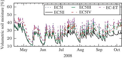
Among the 11 sites, Station 115 stands out, as there are five sensors at the same depth and meteorological data are available. Table 1 provides an overview of these five soil moisture probes. Note that four of the sensors are of one type and that all five are capacitance probes; see Bogena et al. (2007) or Parsons and Bandaranayake (2008) for the dependence on temperature, conductivity and bulk density.

Table 1 Overview of the soil moisture probes

Name	Sensor	Depth	Position
EC5 I	Decagon ECHO EC5	5 cm	Horizontal
EC5 II	Decagon ECHO EC5	5 cm	Horizontal
EC5 III	Decagon ECHO EC5	5 cm	Horizontal
EC5 IV	Decagon ECHO EC5	5 cm	Horizontal
EC-ET	Decagon ECHO EC-TE	5 cm	Horizontal

The data cover more than half of the year 2008 and are shown in Fig. 3. Note that in the graph as well as all subsequent analyses, all days on which the soil temperature is below 3°C are excluded.

Fig. 3 Soil moisture measured by the five sensors at Station 115 of the UDC_SMOS network.

8.2 Exploratory data analysis

There are two very important points to note regarding the time series of the soil moisture measurements in Fig. 3. Firstly, the characteristics of the sensors relative to each other change over time; for instance, the sensors EC5 II and EC5 III give almost identical measurements during May and June; afterwards, the former yields consistently lower values than the latter. This effect is particularly pronounced during the last few weeks, when the spread between the sensors is noticeably bigger. Secondly, the measurements of different sensors are clearly off-set with respect to each other. Whether this is caused by small-scale variability of the soil moisture, soil properties, calibration-related artefacts or other sensor-related issues is not known.

In what follows we will demonstrate how the collocation technique can be applied in an exploratory analysis of the data set. In particular, we will encounter and discuss several pitfalls, which are closely related to the assumptions and structural limitations inherent in the approach.

Pretend that there is reason to believe that the characteristics of probes EC5 II and EC5 III changed during the first half of July and that we are interested in whether such a switch actually occurred. What we are not interested in is whether this imputed change was sudden or gradual in nature. As the sensors appear to have a similar dynamic range over the time-scale of a month, we will apply the bias model equation (23).

The periods, which are assumed to be homogeneous, are defined as follows:

Period 1: 2008-06-01 to 2008-06-30

Period 2: 2008-07-22 to 2008-08-20

Period A1: 2008-05-23 to 2008-05-30

Period A2: 2008-07-14 to 2008-07-21

8.3 Estimation of the calibration constants

We want to investigate the differences of the sensor properties between periods 1 and 2. The periods A1 and A2 are short time windows before these periods; during these, the sensor characteristics are assumed to be the same as in the subsequent period. This allows us to estimate the calibration constants α on a different set of data; thus (assuming no autocorrelation between the errors in the different windows), the estimates are not correlated with the data in the main periods 1 and 2. This separate estimation of the calibration constants and the errors is an expedient way to circumvent the problems described in Section 5.3. We will always give the results of both methods (α estimated in the main periods 1/2 or separately in A1/A2). The constant α is estimated by equation (26), with EC5 III taken to be the reference sensor r.

The resulting values of are as follows:

1. A1 –0.53

2. 1 –0.18

3. A2 –5.22

4. 2 –3.67

The change in bias between the two periods is clearly reflected in the estimates. Note that the differences between periods 1 and A1, as well as between 2 and A2 are rather large, which will have a profound impact on all subsequent results. This could due to lack of stationarity during the time period of interest or random error as the number of measurements is rather small during the A1/A2 period.

If we want to test whether the difference between the estimated α values in periods 1 and 2 is significant, we need to know the error variances. Assuming there is no autocorrelation of the errors between the windows, the at the two periods are uncorrelated. Hence, the variance of the difference is simply the sum of the error variances of at periods 1 and 2, which depend solely on the covariance structure of the error terms. Under the null hypothesis of α at time 1 being equal to α at time 2, we could perform a statistical test to determine whether the deviation of the difference from 0 is significant. A simple parametric test would rely on the error terms being drawn from a Gaussian distribution; would thus also be normally distributed due to linearity. The missing ingredient,however, is the error covariance matrix of sensors EC5 II and EC5 III during both periods. As these are not known, they have to be estimated from the data as well, and the previous test adapted accordingly. Note that this scenario bears a certain resemblance to the Behrens-Fischer problem (Kim and Cohen 1998); however, the estimation of the error variance is much more involved.

8.4 Estimation of variance

First, we will assume that the error terms are mutually uncorrelated, as this is the simplest case imaginable. Bear in mind that the collocation technique has structural limitations: it cannot resolve the complete error covariance structure. However, the availability of five data sources gives us additional information compared to the standard triple collocation approach. In particular, it allows us to form two “independent” estimates of the error variance, where the independence refers to the data sources that are incorporated into the estimator, but whose error terms are not estimated. We will introduce notational shortcuts for the following combinations (the brackets are defined in equation (6):

1. Combination V3i EC5 III, EC-ET; EC5 III, EC5 II, estimates

2. Combination V3ii EC5 III, EC5 IV; EC5 III, EC5 I], estimates

3. Combination VEi EC-ET, EC5 II; EC-ET, EC5 I, estimates

4. Combination VEii EC-ET, EC5 II; EC-ET, EC5 IV, estimates

5. Combination VEiii EC-ET, EC5 I; EC-ET, EC5 IV, estimates

The results are computed by equation (6), with the denominator taken to be (N) when the calibration constant α is estimated from the same data as the variance (from the periods A1/A2), and compiled in Table 2. As both combinations V3i and V3ii provide estimates of , they should give comparable results. However, the differences between the two combinations are large. This as well as the fact that the estimates for combination V3i are negative during Period 2 is an indication that the assumptions could be violated. Two important properties lead to biases: the presence of cross-correlations and autocorrelation. In the latter case, the estimators of the variance become biased because of the influence of the estimated calibration constant, provided it is estimated from the same data. This is the reason why the periods A1 and A2 were introduced. If the autocorrelation persists over longer time scales, even the variance estimated using the calibration constant determined during the A1 (A2) period can become biased due to the temporal proximity of the Period A1 (A2) with the Period 1 (2). The collocation technique can yield estimates of both these terms; however, its usefulness is limited, as shown in the following two sections.

Table 2 Estimated variances

Combination	Period	Period	Result
V3i	1	A1	0.48
V3i	1	1	0.24
V3ii	1	A1	3.58
V3ii	1	1	3.12
V3i	2	A2	−0.67
V3i	2	2	−0.05
V3ii	2	A2	0.70
V3ii	2	2	0.74
VEi	1	A1	2.54
VEi	1	1	2.18
VEii	1	A1	2.65
VEii	1	1	2.02
VEiii	1	A1	6.11
VEiii	1	1	4.07

8.5 Estimation of covariance

The estimated values of are consistently smaller for combination V3i than for V3ii. Under the premise that we expect cross-correlations, if present, to be positive rather than negative, the observed difference could be due to , and deviating from 0. These can be estimated using the following combinations:

1. Combination Ci EC5 III, EC5 I; EC-ET, EC5 IV, estimates

2. Combination Cii EC5 III, EC5 I; EC5 II, EC5 IV, estimates

3. Combination Ciii EC5 I, EC5 II; EC5 IV, EC-ET, estimates

which are chosen such that the corresponding estimators are unbiased if there are no additional non-zero covariances present. They yield the results summarized in Table 3. Note, again, the influence of the period during which the calibration constants α are estimated. They are all positive and their sizes are comparable to the estimated variances of EC5 III and EC-ET; hence, the estimated correlation coefficients are close to one.

Table 3 Estimated covariances

Combination	Period	Period	Result
Ci	1	A1	3.17
Ci	1	1	2.45
Cii	1	A1	2.16
Cii	1	1	1.56
Ciii	1	A1	3.45
Ciii	1	1	2.06

One thus has to face up to the presence of several non-vanishing cross-covariance terms in the error structure. Even though we could extend the data analysis to include more combinations, or to estimate the sensitivity of the results with respect to the choice of the temporal periods, the structural limitations will soon become evident, as only a certain number of assumptions can be relaxed (cf. Section 4).

8.6 Autocovariance

These difficulties carry over to the estimation of the autocovariance function, as shown in Fig. 4, where the notation established in Section 8.4 applies. The differences seen for , i.e. the usual error variance (numerical values are given in Table 3), are also evident at non-zero lags; the results obtained with combination V3iii are consistently higher than those obtained with either V3i or V3ii. In this case, the results are also much more influenced by the way the calibration constant α is estimated.

Fig. 4 Different estimates of (a) the autocovariance and (b) the auto-cross-covariance function of sensor EC-ET. The legend refers to the combination and the period during which α is estimated, e.g. V3i/A1 denotes the estimate with combination V3i, where α was determined during period A1.

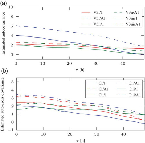
8.7 Auto-cross-covariance

The Auto-cross-covariance functions , and are plotted in Fig. 4. The combinations are those already employed in Section 8.5, and the numerical values for are compiled in Table 2. The most important aspect to notice is that the decay of the cross-covariances occurs at different time scales. This hints at the possibilities the collocation technique offers for comparing the temporal characteristics of data products, if the structural limitations can be overcome by an appropriate choice of data sources and assumptions.

8.8 Summary

The structural deficencies of the collocation technique are illustrated at the hand of a larger number of data sets than usually employed. These difficulties, which are present in both the estimation of the error variance and the autocovariance, render the testing of a simple hypothesis regarding this data set virtually impossible as they can only be mitigated with the introduction of additional assumptions.

9 CONCLUSIONS

The comparison of different data sets, such as models and measurements, is exceedingly common, as it is a crucial step in the validation of these products, as well as the analysis of geophysical phenomena. In the area of soil moisture research, the dissimilarities between the data sources are often highly complex (Entekhabi et al. 2010): the means, dynamic ranges and error properties are different and potentially change over time, thus necessitating inter-sensor calibration. The collocation technique yields estimates of the error variance in the presence of these off-sets. The estimators, however, become biased if the errors are autocorrelated, as might occur when the models are flawed, e.g. a systematic deviation present that persists over time. This temporal autocorrelation is closely connected to time-varying calibration constants, which account for the different means and dynamic ranges. Case study 1 (Section 7) showed the presence of autocorrelated errors and temporal changes in the calibration constants in three soil moisture data sets. This complex temporal behaviour limits the applicability of many techniques, not least the standard triple collocation method, as these tend to rely on very stringent assumptions that often do not apply in real data sets. The estimation of the autocorrelation, time-variant inter-sensor calibration and error properties can thus potentially enrich the analysis and comparison of different kinds of measurements and models, and thus improve the understanding of these products. The error autocorrelation might not be of particular interest in itself in certain studies, but its connection to the temporal variations of the characteristics of different data sets (such as the mean), make it a valuable component in the analysis of the variability of, for example, the scaling properties of soil moisture, the analysis of remote sensing products or for sensitivity studies comparing different calibration approaches.

Acknowledgements

The authors would like to thank the anonymous reviewers for their helpful comments which improved the quality of the manuscript considerably.

Notes

1. ¹One possible solution for the mitigation of this problem would be data thinning, i.e. only looking at measurements whose temporal distance exceeds the correlation length.

REFERENCES

- Bogena, H., et al., 2007. Evaluation of a low-cost soil water content sensor for wireless network applications. Journal of Hydrology, 344 (1–2), 32–42.
- Caires, S. and Sterl, A., 2003. Validation of ocean wind and wave data using triple collocation. Journal of Geophysical Research, 108 (C3), 3098–3114.
- Dee, D.P., et al., 2011. The ERA-Interim reanalysis: configuration and performance of the data assimilation system. Quarterly Journal of the Royal Meteorological Society, 137 (656), 553–597.
- Dorigo, W., et al., 2010. Error characterisation of global active and passive microwave soil moisture datasets. Hydrology and Earth System Sciences, 15, 425–436.
- Dorigo, W.A., et al., 2011. The international soil moisture network: a data hosting facility for global in situ soil moisture measurements. Hydrology and Earth System Sciences, 15 (5), 1675–1698.
- Entekhabi, D., et al., 2010. Performance metrics for soil moisture retrievals and application requirements. Journal of Hydrometeorology, 11 (3), 832–840.
- Habib, E., Aduvala, A., and Meselhe, E., 2008. Analysis of radar-rainfall error characteristics and implications for streamow simulation uncertainty. Hydrological Sciences Journal, 53 (3), 568–587.
- Hain, C., et al., 2011. An intercomparison of available soil moisture estimates from thermal infrared and passive microwave remote sensing and land surface modelling. Journal of Geophysical Research, 116, D15107.
- Hossain, F. and Huffman, G., 2008. Investigating error metrics for satellite rainfall data at hydrologically relevant scales. Journal of Hydrometeorology, 9 (3), 563–575.
- Kim, S.-H. and Cohen, A., 1998. On the Behrens-Fischer problem: a review. Journal of Educational and Behavioral Statistics, 23 (4), 356–377.
- Koopmans, L., 1995. The spectral analysis of time series. San Diego, CA: Academic Press.
- Koster, R. and Milly, P., 1997. The interplay between transpiration and runoff formulations in land surface schemes used with atmospheric models. Journal of Climate, 10 (7), 1578–1591.
- Koster, R. and Suarez, M., 2001. Soil moisture memory in climate models. Journal of Hydrometeorology, 2 (6), 558–570.
- Loew, A. and Schlenz, F., 2011. A dynamic approach for evaluating coarse scale satellite soil moisture products. Hydrology and Earth System Sciences, 15, 75–90.
- Miralles, D., Crow, W., and Cosh, M., 2010. Estimating spatial sampling errors in coarse-scale soil moisture estimates derived from point-scale observations. Journal of Hydrometeorology, 11, 1423–1429.
- Naeimi, V., et al., 2009. An improved soil moisture retrieval algorithm for ERS and METOP scatterometer observations. IEEE Transactions on Gesocience and Remote Sensing, 47 (7), 1999–2013.
- O’Carroll, A., Eyre, J., and Saunders, R., 2008. Three-way error analysis between AATSR, AMSR-E, and in situ sea surface temperature observations. Journal of Atmospheric and Oceanic Technology, 25 (7), 1197–1207.
- Parlange, M., et al., 1992. Physical basis for a time series model of soil water content. Water Resources Research, 28 (9), 2437–2446.
- Parrens, M., et al., 2012. Comparing soil moisture retrievals from SMOS and ASCAT over France. Hydrology and Earth System Sciences, 16, 423–440.
- Parsons, L. and Bandaranayake, W., 2008. Performance of a new capacitance soil moisture probe in a sandy soil. Soil Science Society of America Journal, 73, 1378–1385.
- Rehfeld, K., et al., 2011. Comparison of correlation analysis techniques for irregularly sampled time series. Nonlinear Processes in Geophysics, 18, 389–404.
- Reinsel, G., 1997. Elements of multivariate time series analysis. New York: Springer-Verlag.
- Sánchez, N., et al., 2012. Validation of the SMOS L2 soil moisture data in the REMEDHUS network (Spain). IEEE Transactions on Gesocience and Remote Sensing, 50 (5), 1602–1611.
- Schlenz, F., et al., 2012. Uncertainty assessment of the SMOS validation in the Upper Danube catchment. IEEE Transactions on Gesocience and Remote Sensing, 50 (5), 1517–1529.
- Scipal, K., et al., 2008. A possible solution for the problem of estimating the error structure of global soil moisture data sets. Geophysical Research Letters, 35, L24403.
- Shiklomanov, A., et al., 2006. Cold region river discharge uncertainty estimates from large Russian rivers. Journal of Hydrology, 326, 231–256.
- Stoffelen, A., 1998. Toward the true near-surface wind speed: error modeling and calibration using triple collocation. Journal of Geophysical Research, 103 (C4), 7755–7766.
- Western, A., et al., 2004. Spatial correlation of soil moisture in small catchments and its relationship to dominant spatial hydrological processes. Journal of Hydrology, 286, 113–134.
- Winterfeldt, J., et al., 2010. Comparison of HOAPS, QuikSCAT, and buoy wind speed in the Eastern North Atlantic and the North Sea. IEEE Transactions on Gesocience and Remote Sensing, 48 (1), 338–348.
- Zwieback, S., et al., 2012a. Structural and statistical properties of the collocation technique for error characterization. Nonlinear Processes in Geophysics, 19 (1), 69–80.
- Zwieback, S., Dorigo, W., and Wagner, W., 2012b. Temporal error variability of coarse scale soil moisture products—case study in central Spain. In: Proceedings of the international geoscience and remote sensing symposium. Munich: IEEE, 722–725.