Forecasting flash floods using data-based mechanistic models and NORA radar rainfall forecasts

Abstract

Data-based mechanistic (DBM) models can offer a parsimonious representation of catchment dynamics. They have been shown to provide reliable accurate flood forecasts in many hydrological situations. In this work, the DBM methodology is applied to forecast flash floods in a small Alpine catchment. Compared to previous DBM modelling studies, the catchment response is rapid. The use of novel radar-derived ensemble quantitative precipitation forecasts based on analogues to drive the DBM model allows the forecast horizon to be increased to a level useful for emergency response. The characterization of the predictive uncertainty in the resulting hydrological forecasts is discussed and a framework for its representation illustrated.

Editor Z.W. Kundzewicz; Guest editor R.J. Moore

Citation Smith, P.J., Panziera, L., and Beven, K.J., 2013. Forecasting flash floods using data-based mechanistic models and NORA radar rainfall forecasts. Hydrological Sciences Journal, 59 (7), 1343–1357. http://dx.doi.org/10.1080/02626667.2013.842647

Résumé Les modèles mécanistes fondés sur les données (en anglais, data-based mechanistic—DBM) peuvent offrir une représentation parcimonieuse de la dynamique du bassin versant. Il a été montré qu’ils fournissent des prévisions de crue fiables et précises dans de nombreuses situations hydrologiques. Dans ce travail, la méthodologie DBM est appliquée pour prévoir des crues éclair dans un petit bassin versant alpin. Par rapport aux études antérieures de modélisation DBM, la réponse du bassin versant est rapide. L’utilisation de nouvelles prévisions quantitatives d’ensemble de précipitations, dérivées du radar et basées sur des analogues pour forcer le modèle DBM, permet d’accroître l’horizon de prévision à un niveau utile pour les interventions d’urgence. La caractérisation de l’incertitude prédictive dans les prévisions hydrologiques résultantes est discutée et un cadre pour sa représentation est illustré.

Key words:

• DBM
• NORA
• flash flood forecasting

Mots clefs:

• DBM
• NORA
• prévision des crues éclair

Introduction

The issuing of timely flood alerts requires the ability to predict future values of water level or discharge at vulnerable points within a catchment. These predictions must be available with a lead-time that allows successful application of suitable mitigating responses: for example the issue of warnings to the public or the deployment of portable flood defences. For flooding in catchments where there is adequate delay in the response to rainfall, suitable predictions can often be achieved using only observed data (see for example Romanowicz et al. 2006, 2008). In contrast, flash floods are characterized by rapid natural response times typically less than the lead-time required for the application of mitigating measures. Extending the lead-time of flash flood forecasts requires not only the hydrological forecasting problem (predicting the water level or discharge at points of interest) to be addressed, but also the meteorological forecasting problem that is predicting the future precipitation.

Recently, the use of ensemble precipitation forecasts in hydrology has attracted much attention (see for example Schaake et al. 2007, Cloke and Pappenberger 2009, Dietrich et al. 2009, Thielen et al. 2009). A number of papers have specifically addressed flash flood forecasting (see for example Beven et al. 2005, Zappa et al. 2008, Rotach et al. 2009, Rossa et al. 2011). This paper takes a similar approach to these, in that precipitation predictions are used to drive a hydrological model which produces forecasts of future river discharge. However, tools not previously used within this context are introduced. The techniques presented are outlined through application to the Verzasca catchment (Ticino, Switzerland).

Methods for generating quantitative precipitation forecasts (QPF) can be categorized into four main types: those based on extrapolation of radar fields (e.g. Germann and Zawadki 2002); those from numerical weather prediction (NWP) models (e.g. Marsigli et al. 2005, 2008); those from stochastic models of rainfall evolution (e.g. Sirangelo et al. 2007); and those derived from historical analogues (e.g. Duband 1970, Obled et al. 2002). The temporal extrapolation of weather radar fields offers the potential for forecasts with a level of spatial resolution that is not currently generally achievable through NWP models. The lower computational cost compared to NWP also allows forecasts to be issued more frequently based on the most recent meteorological observations. However, the level of accuracy achieved by radar-based QPF can decay rapidly (Germann et al. 2006a). In part, this is due to limitations in the techniques used to predict the growth and dissipation of rainfall and changes in the air flow direction. For a comprehensive evaluation of an extrapolation technique over a complex-orography region see Mandapaka et al. (2012).

In this study, ensemble QPF based on radar rainfall data are provided by NORA (Nowcasting Orographic Rainfall by means of Analogues; Panziera et al. 2011). NORA precipitation forecasts are derived from historical analogues and so avoid the need to explicitly model the evolution of the rainfall field.

The QPFs are used to drive a hydrological model formulated with the data-based mechanistic (DBM) modelling approach. This inductive modelling approach is based on the identification and estimation of a numerical representation of a catchment that reflects the catchment dynamics using a minimum degree of model complexity identified directly from the available data. The DBM process imposes a further requirement in that the resulting model structure and parameterization must have a mechanistic interpretation (for example as a series of tanks) that does not contradict the perceptual model of the analyst. Fuller discussions of the DBM approach to modelling, the value of the mechanistic interpretation in guarding against erratic model behaviour when forecasting, along with further hydrological applications can be found in Young (2001, 2002, 2003, 2006), Young et al. (2004) and Lees et al. (1994).

The DBM model formulation considered herein offers the potential for the assimilation of data into the hydrological model to improve its forecasts. This is undertaken to improve deterministic model forecasts. The distribution of the observed discharge that may be witnessed for a given forecast value is characterized using a non-parametric copula formulation of their joint distribution. The use of copulas for analysis of multivariate hydrological problems has received much attention (see Song and Singh 2010 and the references within). Previously published hydrological studies have made use of parametric copulas to characterize predictive uncertainty (see for example Krzysztofowicz 1999, Montanari and Brath 2004, Todini, 2008). Other uses for copulas have been the estimation of extreme events (e.g. Salvadori and De Michele 2007, Keef et al. 2009) and spatial correlations (e.g. Bàrdossy and Li 2008).

THE VERZASCA CATCHMENT AND DATA AVAILABILITY

The techniques presented are demonstrated by application to the Verzasca basin, located in the Ticino region of southern Switzerland. This catchment has been used in a number of other flash flood forecasting studies (see Zappa et al. 2011 and the references within). The lower part of the catchment is dominated by a reservoir controlled by the Verzasca Dam, which is used for hydroelectric power generation. This study focuses on forecasting discharge at a gauging site above the reservoir.

Above the gauge, the catchment is an alpine basin of 186 km² with an elevation range of 490–2870 m a.m.s.l. The predominant land covers are forest (30%), shrub (25%), rocks (20%) and alpine pastures (20%). Snowmelt governs the discharge regime in spring and early summer. Heavy autumnal rainfall events coupled with steep valley sides and shallow soils (generally less than 30 cm) make the Verzasca River prone to flash floods. Further details can be found in Ranzi et al. (2007) and Wöhling et al. (2006).

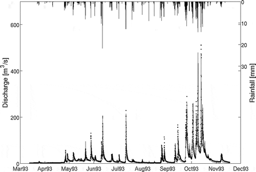
Observed discharge data at an hourly time-step are available at the gauged site from 1990. These, rather than the corresponding observed level series, are modelled, despite the drawbacks (e.g. Romanowicz et al. 2006, Beven et al. 2011), since the rated cross-section at the gauging site has altered during the observation period resulting in a non-stationary level series. Note, as is common in such catchments, the typical peak flood discharge of 400 m³/s should be treated with some caution since no observation greater than 100 m³/s is used in deriving the rating curve. Meteorological records for a corresponding time period are available from up to six locations in the surrounding area. These are used to derive catchment-averaged rainfall and temperature series at an hourly time-step.

NORA QUANTITATIVE PRECIPITATION FORECASTS

Nowcasting of Orographic Rainfall by means of Analogues (NORA) is an analogue-based heuristic nowcasting system for short-term forecasting of orographic precipitation (Panziera et al. 2011). It is based on the repeatability of the rainfall patterns observed in the mountains given certain environmental conditions, due to the presence of the orographic forcing (Panziera and Germann 2010). The basic concept of NORA is to look into the past for analogues, i.e. the past situations with mesoscale flows, air mass stability and rainfall patterns most similar to those observed at the current instant. The rainfall accumulated in the hours following the analogues is then used for the quantitative precipitation forecasts. Growth and decay of rainfall, which are not accounted for by Lagrangian extrapolation methods, are automatically taken into account by NORA, since the forecasts are generated from past observed rainfall fields.

The predictors

The quantities estimated in real-time and used by NORA to find the analogues in the historical archive (predictors) are four mesoscale flows, air mass stability, and two characteristics of the radar image: wet area ratio and image mean flux (for a detailed description, see Panziera et al. 2011).

The MeteoSwiss weather radar located on the top of Monte Lema (1625 m a.s.l.), one of the southernmost mountains of the Alpine ridge in the Lago Maggiore region, is used to estimate ground-level rainfall and mesoscale winds. The radar rainfall estimate is obtained by the operational MeteoSwiss radar product for quantitative precipitation estimation (QPE). This represents a best estimate of precipitation at the ground derived by correcting the radar image to observed rainfall gauge data (Germann et al. 2006b). The horizontal spatial resolution of the precipitation map is 1 km × 1 km and the temporal resolution is 5 min. Wet area ratio is defined as the fraction of wet area in the radar image (using a threshold of 0.16 mm/h) and image mean flux is the average rainfall of the image.

The mesoscale wind is estimated by Doppler velocity measurements, which have a spatial resolution of 1° in azimuth and 1 km in range and are also updated every 5 min. In particular, four mesoscale winds are estimated at different heights in various regions of the radar volume scan, by fitting a linear wind to the measurements taken in some pre-defined regions of interest.

Air mass stability (as represented by the moist Brunt-Väisälä frequency) is estimated from a pair of adjacent automated meteorological ground stations: Stabio (353 m) and Monte Generoso (1608 m). These stations are located on the first slopes of the Alps very close to the Po Valley at different altitudes.

Historical cases

Seventy-one (71) precipitation events observed in the Lago Maggiore region from January 2004 to December 2009, corresponding in total to 127 days of precipitation (3050 h), constitute the historical archive within which NORA searches for the analogues. Table 1 shows the temporal distribution of the events. The majority of events occur at times when heavy precipitation can be expected to cause a significant discharge response in the Verzasca catchment. The choice of these events resulted from a trade-off between the following three requirements. First, the dataset in which the analogues are searched should be as large as possible. Second, the archive has to be homogeneous to avoid artefacts of instrumental changes and different data processing techniques. Third, long-lasting and widespread events typically caused by a large-scale supply of moisture towards the Alps should be selected, as the orographic forcing is the main mechanism that regulates precipitation in these cases. Moreover, isolated convection and air mass thunderstorms, which are less extended in space and time, rarely result in critical amounts of rainfall falling on the Verzasca catchment. Details about the choice of the rainfall events are given in Panziera and Germann (2010, Section 2.2).

Table 1 Occurrence of NORA events summarized by year and month. Zero values are left blank

Month	Year						Total
	2004	2005	2006	2007	2008	2009
January					1		1
February
March		1		1			2
April	2	1	1		4	2	10
May	1	5	1	3			10
June		3		2	1	2	8
July		2		1	1		4
August	2	2	1	2	2	4	13
September	1	2	2	1	2	1	9
October	2	1	1			2	6
November	1		1	1	2	1	6
December			1			1	2
Total	9	17	8	11	13	13	71

The forecasting method

The analogues are identified through a two-step process: first, 120 analogues from the predictors that describe the orographic forcing are obtained; second, the 12 analogues with the radar image most similar to the current one are selected among the 120.

The analogue model employed by NORA makes use of a scaled Euclidean distance computed in a multidimensional space. The coordinates of such space are the zonal and meridional components of the four mesoscale flows and air mass stability in the first step, and wet area ratio, image mean flux and their variation in the two previous hours in the second step. The conditions with the smallest distances are assumed to be the most similar to the current situation (i.e. analogues).

A 12-member ensemble forecast is generated. Of the 12 members, 11 correspond to historic analogues and the final one to the current time-step. Forecast members derived from the 11 historic cases are the rainfall fields observed after the time of the selected analogue. The forecast member generated from the current time-step assumes persistence. Forecasts with a time-step of 5 min, a spatial resolution of 1 km² and a lead-time of up to 8 h can be produced by NORA. Forecasts (based on computing both sets of analogues) can be issued every 5 min. For the purposes of this study, NORA forecasts of the catchment-averaged rainfall over the Verzasca basin on an hourly time-step were issued every hour.

NORA versus persistence and COSMO2

In order to evaluate the performance of NORA for the Verzasca Valley, skill scores of NORA, Eulerian persistence and COSMO2 are presented in Fig. 1. The gauge-adjusted QPE derived from the radar is assumed to be the ground truth. Eulerian persistence is a simple forecasting technique which considers the last radar image as the forecast for any lead-time, and it is often regarded as the simplest reference forecasting method. COSMO2 is the limited-area non-hydrostatic numerical model, used operationally at MeteoSwiss, that has a spatial resolution of 2.2 km, an updating frequency of 3 h and a forecast range of 24 h.

Fig. 1 Summary of the performance of the hourly accumulated NORA precipitation forecasts against those generated by persistence and COSMO2 at lead-times of up to 6 h. For a definition of the verification scores presented, see Wilks (1995) and Panziera et al. (2011). Lead-time is given as the start of the accumulation period.

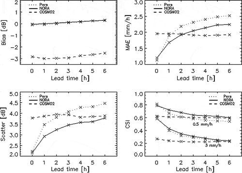
The verification was performed for a subset of the historical archive, given by the precipitation events that occurred after May 2007, corresponding to a total of 14 535 samples. The temporal resolution of the verification dataset is 5 min. The forecasts are verified only within the Verzasca catchment. Figure 1 presents the verification of predictions of hourly accumulated rainfall with a lead-time of up to 6 h, derived by the average of the 12 NORA ensemble members. In order to evaluate the skill of NORA in real-time mode, the 24 h following the sample for which the forecast was made were excluded from the historical archive in which the analogues are searched. For a definition of the verification scores presented in Fig. 1, see Wilks (1995) or Panziera et al. (2011).

Figure 1 shows that COSMO2 suffers from a large negative bias, whereas NORA and persistence are almost unbiased. In terms of mean absolute error, however, NORA is better than COSMO2 up to a lead-time of 2 h, whereas for longer lead-times the numerical model gives better forecasts. However, NORA is better than the other forecasting systems when considering the “Scatter” measure, which describes the variability of the agreement between forecasts and observations (see Germann et al. 2006b), and the CSI measure, which expresses the ability of the system to have high probability of detection (POD) and low false alarm rate (FAR), and is calculated for two rain-rate thresholds (0.5 and 3 mm/h). In general, Fig. 1 shows that the hourly accumulated NORA rainfall forecasts are similar to Eulerian persistence if the lead-time is 0 (i.e. accumulation starts at the time the forecast is issued), but closer to the reality with respect to persistence for longer lead-times. For a more comprehensive verification of NORA over the Largo Maggiore region, see Panziera et al. (2011).

DATA-BASED MECHANISTIC MODEL OF THE VERZASCA

This section presents the derivation of a deterministic DBM forecasting model for the Verzasca catchment. A parsimonious model of the catchment is identified, and its parameters estimated with reference to the available data. In keeping with the DBM modelling methodology, the model selected must not just optimize some (predefined) criteria of statistical optimality, but must also be interpretable as a physical system. This interpretability can be contrasted against the perceptual model of the system. This gives the modeller a criterion on which to reject models that, though fitting the observed data, may appear physically unreasonable.

To illustrate this, consider the DBM model formulation in equation (1), commonly used in rainfall–runoff modelling:

(1)

The discharge volume observed within the tth time-step, y_t, is predicted as the sum of a “baseflow” component, estimated as the minimum of the calibration discharge series y_min, a stochastic noise ϵ_t and the supposition of rainfall responses defined by the second term in the right-hand side of equation (1). The response to the rainfall r_t−d is determined by two components. The first is the discrete time linear transfer function (defined using the backward shift operator z⁻¹, such that z⁻ⁱy_t = y_t−i), which represents a scaled unit hydrograph. The second is the gain function f(y_t−d), which scales the rainfall to an effective value. This is often taken to be a function of the discharge, since it can act as a surrogate for catchment wetness (Young and Beven 1994). The integer time delay d allows for an advective time delay within the system and for the computation of the effective input f(y_t-d)r_t-d to be performed using observed data.

Identification of the model in equation (1) corresponds to the selection of the structure of the linear transfer function (m,n,d) along with the function f, whose parameters along with (a₁, …, a_n,b₀, …, b_m) require estimation. To ensure the mechanistic interpretation outlined above, the identified and estimated impulse response of the linear transfer function must be positive at all time steps and f(y_t-d) should be monotonically increasing.

Model identification and estimation

The DBM model for the Verzasca catchment is constructed offline using historical data from 1990 to 2003. The DBM model is evaluated on a 1 hour time-step for compatibility with the observed hydrological and meteorological data which consists of discharge volumes y = (y₁, … , y_T) along with catchment averaged temperatures k = (k₁, … , k_T) and precipitation totals u = (u₁, … , u_T). Since the time period pre-dates the availability of radar-derived QPE a catchment-averaged precipitation derived from gauge data is used.

Analysis of the system proceeded by fitting a linear discrete time transfer function driven by precipitation to the observed output data minus its minimum value y_min. In fitting, a number of structures of the linear transfer function were tried. For each structure the parameters (a₁, … , a_n,b₀, … , b_m) were estimated using the refined instrument variable algorithm (Jakeman and Young 1979, Young and Jakeman 1979). An optimal model structure was selected using the YIC (Young et al. 1980), an information criterion that trades off parameter identifiably, assessed using the covariance of the parameter estimates, and the fit of the model to the data.

The residuals of this initial model suggested that the relationship between the precipitation input and the observed discharge was nonlinear. As found in previous studies of the Verzasca (e.g. Ranzi et al. 2007), the nonlinearity is heavily influenced by precipitation falling as snow and its subsequent melting. In a past DBM modelling study covering the Ticino region (Young et al. 2007), a transformed temperature series was used as a second input in a multiple-input single-output (MISO) transfer function to capture the dynamics of this behaviour. This proved inadequate in this more detailed study.

To proceed further, a method for separating the input signal due to snowmelt (v_t) and a rainfall input (r_t) is required. The following model evolving the snow store s_t may be used:

1. If k_t ≥ 0 then r_t = u_t, s₊ = 0 and the fraction of the snow store melted is: ;

2. If k_t < 0 then r_t = 0, s₊ = u_t, and f_t = 0;

3. Evaluate s_t+1 = (1 – f_t)s_t + s₊ and v_t = f_ts_t.

The value of θ_t is given by a sinusoid function whose annual maximum was set for 21 June and minimum for 21 December, thus providing a crude representation of seasonal variation in solar radiation (Braun 1985). The values of γ and s_max require estimation from the observed data.

The snowmelt model can be seen as an application of the positive degree-day index (PDDI) methodology, with the fraction of catchment surface area covered in snow proportional to s_t up to some storage volume s_max when the whole catchment surface area is covered. The relationship to PDDI models allows a mechanistic interpretation of the separation of the input signal, even though the nature of the remainder of the model implies that they should not be taken explicitly as snowmelt and rainfall volumes.

Exploration of any further input nonlinearity that may be required was performed using non-parametric state-dependent parameter estimation (Young et al. 2001). This allows the form of, and need for, a gain function (f in equation (1)) to be explored by considering the dependency of (b₀, … , b_m) on an observed variable such as the discharge. This indicated that, in keeping with past studies (e.g. Young and Beven 1994), the response to the rainfall requires a gain function whose value should increase as y_t (at a corresponding time to the input) increases. This suggests that rain falling on a wet catchment (indicated by high discharge) produces more of an effect on the future discharge than a similar volume of rain falling on a drier catchment. The response to the snowmelt input shows a similar pattern, but is poorly defined for higher discharges where limited periods of snowmelt are observed.

Following the non-parametric analysis, the model structure shown in equation (2) is proposed. The gain functions for the two input series are parameterized as powers of the observed discharge. The effective input series are related to the observed discharge by a MISO linear transfer function with a common denominator polynomial and stochastic noise series υ_t.

(2)

The gain functions control the shape of the gain for the given inputs. The actual gain can be computed from the total response to a unit input by taking account of the measurement units. The total response can be computed without recourse to simulations, since, in the case of rainfall, a unit input produces a total response of:

(3)

The parameters (φ_r,φ_v,γ,s_max) were optimized by a grid search with the aim of minimizing . The optimal structures of the linear transfer function were identified and estimated for each point on the grid search using the techniques already discussed. The values of (φ_r,φ_v,γ,s_max) were computed as (0.35,0.5,0.65,865). The corresponding linear transfer function structure selected was (n,m_r,m_v,d_r,d_v) = (2,2,2,2,2).

Substituting the estimated parameter values into equation (2) and performing a partial fraction decomposition on the linear transfer functions allows the model to be expressed as:

(4)

This component of the model can now be mechanistically interpreted as representing two pathways of response. Each pathway is characterized by a linear tank expressed as a first order MISO output linear transfer function. The time constants of the tanks can be computed from the time-step of the model (1 h) and the single a parameter of the first-order transfer function. For the model in equation (4) the time constants are –1/log(0.9929) = 139.5 h and –1/log(0.8313) = 5.4 h, indicating distinct slow and fast response paths. The ratios of the numerator parameters of the two first-order transfer functions for an effective input determine how that input is split between the pathways. The effective rainfall input is split so that 96% goes to the fast pathway in comparison with 99% for the effective snowmelt . Figure 2 shows the model simulated discharges over the calibration period and which account for 87% of the variance in the observations.

Fig. 2 One year of calibration data showing the observed data (•) and simulated DBM output (––––).

State space model and data assimilation

The model presented in equation (4) could form the basis of the forecasting system. However, assimilation of observed water levels to the DBM model may improve the forecasts given. As in past DBM modelling studies (e.g. Young 2002, Romanowicz et al. 2006, 2008), data assimilation is performed by casting the linear transfer function in a state space form and embedding it in the Kalman filter.

A state space form corresponding to the two parallel paths of response is selected. The state vector x_t consists of two states, corresponding to volumes of water in each path, and evolves according to:

(5)

(6)

(7)

The notation ζ_t+1 ˜ (0,Qλ₀) (for example) indicates that ζ_t+1 is distributed with mean 0 and covariance Qλ₀. The matrices A and B are given by:

(8)

and h = [1 1]^T.

The parameters (Q,λ₀,λ₁,λ₂) describe the stochastic noise terms denoted by Greek letters in equations (5) and (6). The matrix Q is taken to be diagonal so indicates the relative level of noise applied to each response path. The formulation for the observation variance in equation (6) has a state dependency described in equation (7) (see Young 2002, Romanowicz et al. 2006, Smith et al. 2008). This recognizes that both predictions and observations of high discharges are more uncertain. Formulating the state space model is this way, without the snow store s_t in the state vector, means the computation of the effective inputs will not be altered by assimilating data.

Suppose the state vector x_t is unknown and can be summarized by its mean and variance P_tγ₀; the Kalman filter can now be used for updating the summary statistics of the state distribution as observations become available. Using the subscript t + 1|t to indicate the prediction of time-step t + 1 given all the information up to and including time-step t, the a priori prediction equations are:

(9)

(10)

Following the observation of , the a posteriori correction is computed using:

(11)

(12)

(13)

The expected value of the f-step ahead predictions are given by and the corresponding prediction variance by . The values of and can be computed by repeated application of the a priori steps of the Kalman filter given by equations (9) and (10).

The Kalman filter recursions are an optimal assimilation strategy for linear systems if it can be assumed that ξ_t+1 and ζ_t+1 are independent random variables and their distributions, along with that of the state vector, are unbounded and symmetric. In many applications, such as this where the states only maintain a physical meaning if they are positive, these assumptions are not valid. Even when these assumptions do not hold, the Kalman filter may still provide an approximate assimilation scheme which is useful in practice (e.g. Young 2002).

Forecasting within the time delay of the model (that is f ≤ min(d_r,d_v)) requires no forecast inputs. This is the situation most often considered in previous hydrological studies using DBM models (e.g. Young 2002). In such circumstances, the variance parameters of the Kalman filter can be optimized for the given lead-time against some criteria assessing the predictive performance. For example, presuming the observations follow independent Gaussian distributions with mean and variances , the likelihood of the f-step ahead predictions can be computed and maximized (e.g. Smith et al. 2008).

Romanowicz et al. (2006, 2008) used similar techniques in DBM modelling studies where forecast inputs (in this case river levels) are used to extend the available forecast lead-time of a downstream water level. Long periods (>5 years) of forecast input data were available. These allowed the calibration of Kalman filter variance parameters. In this study, such long time periods of meteorological forecasts are not available. Even if they were (see for example the COSMO-LEPS data used in Alfieri et al. 2011), the meteorological model may have undergone several revisions. This suggests that the nature of the meteorological forecast errors may have evolved complicating the calibration of the Kalman filter variance parameters.

In the following section, the uncertainty of the forecast of the future observed discharge is captured by representation of the joint distribution of the observed data and a deterministic forecast. The expected values of the forecast given by the Kalman filter are utilized as the deterministic forecast. Since the expected value of the forecast is independent of λ₀, it can be left unspecified, though a maximum-likelihood estimate can always be computed (Schweppe 1965). For each lead-time (Q,λ₁,λ₂) are optimized to minimize the sum of squared errors of the expected value of the forecasts. For the purposes of this calibration step, future observations of the precipitation and temperature are presumed to be available where required so forecasts can be generated for lead-times beyond the time delay of the model. Therefore, the model is estimated as though the predictions of precipitation exactly matched what was later observed. To compute the effective inputs where observed values of the discharge are unavailable, they were replaced by the most recent forecast value. Smith et al. (2013) present a method of correctly characterizing the forecast variance in such situations.

Table 2 Summary statistics of forecasting performance during calibration of the DBM model using data assimilation with the assumption that future rainfall is known. Values in parentheses represent the statistics computed only when discharge >75 m³/s. Results for the model run without data assimilation are shown for comparison

Lead time	RMSE	Bias	Kendall tau
(h)	(m^3/s)	(m^3/s)
No data assimilation	7.94 (48.6)	1.56 (10.7)	0.76 (0.55)
1	2.92 (19.6)	0.02 (0.45)	0.98 (0.83)
2	4.59 (30.9)	0.04 (1.04)	0.96 (0.73)
3	5.74 (38.2)	0.05 (1.50)	0.95 (0.66)
4	6.64(44.0)	0.06 (1.80)	0.93 (0.61)
5	6.79 (44.6)	0.30 (5.26)	0.92 (0.60)
6	7.27 (47.6)	0.35 (6.14)	0.91 (0.58)

Table 3 Summary statistics of forecasting performance during validation of the DBM using data assimilation with the assumption that future rainfall is known. Values in parentheses represent the statistics computed only when discharge >75 m³/s

Lead-time	RMSE	Bias	Kendall tau
(h)	(m^3/s)	(m^3/s)
1	3.32 (29.1)	0.02 (0.02)	0.98 (0.82)
2	5.46 (47.9)	0.04 (0.24)	0.96 (0.71)
3	7.10 (62.2)	0.05 (0.69)	0.94 (0.64)
4	8.22 (71.8)	0.07 (1.21)	0.93 (0.60)
5	7.91 (67.8)	0.32 (9.75)	0.92 (0.57)
6	8.23 (69.9)	0.38 (11.9)	0.91 (0.54)

Table 2 summarizes the calibration performance of the model for various lead-times. The results of the model, in effect a 2-h ahead forecast, without data assimilation, are shown for comparison. At all lead-times the data assimilation strategy improves (lowers) the RMSE and bias of the forecasts. The improvement due to data assimilation is particularly marked at higher discharges and shortened lead-times. The RMSE and bias measure the magnitude of the forecast errors. However, due to the transformations used, copula formulations are in general not sensitive to magnitude errors but are sensitive to changes in the relative rank of time-steps in the forecast and observed data series. The final performance statistic shown in Table 2, Kendall tau, indicates that the rank correlation is also improved by the data assimilation.

Figure 3 gives a visual impression of the effect of the data assimilation on the forecasts issued. Table 3 replicates the performance summary in Table 2 for a validation period between 2004 and 2008. The performance of the model forecasts is broadly similar to that witnessed during calibration, though, in general, there is a slight decrease in the quality of the forecasts.

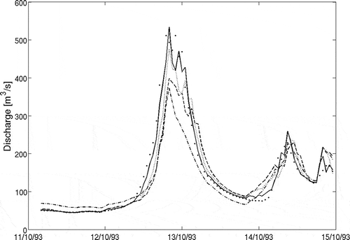
Fig. 3 Calibration forecast (made using observed rainfall) for a large event in the autumn of 1993. Observed data (•) and forecasts using data assimilation at lead-times of 1 h (–––), 3 h (......) and 5 h (- - - -) are shown together with the model output using no data assimilation (- . - . -).

GENERATING PROBABILISTIC FORECASTS

The generation of deterministic discharge forecasts using data assimilation when values of the precipitation and temperature are known has been discussed in the previous section. In the case of the Verzasca region, this means that deterministic forecasts of up to 2 h lead-time can be issued. Generating probabilistic forecasts from these is therefore a matter of characterizing the joint distribution of the forecast and observed data at each lead-time. For longer lead-times, the effects of substituting the NORA precipitation forecasts for the observed data need to be considered.

A strategy taken by a number of authors (Kelly and Krzysztofowicz 2000, Herr and Krzysztofowicz 2010, Smith and Beven 2010, Alfieri et al. 2011) is to construct two distributions. The first distribution, based on the hydrological model, is that of the observed discharge given the observed precipitation. The second distribution gives the probability of the observed precipitation given the meteorological forecasts. Significant difficulties are present in the construction of the predictive distribution of the precipitation, particularly in forecasting the timing of precipitation events and events that are not forecast by the meteorological model. Smith et al. (2012) constructed the joint distribution of the observed data and the hydrological forecasts that result from evolving the hydrological model with each member of the ensemble precipitation forecast. The basis of this approach is that the hydrological model acts as a low pass filter of the rainfall, and the joint distribution of resulting forecasts may be more easily characterized. The added complexity of characterizing this multivariate distribution appears unwarranted given the limited data available for this study (Smith et al. 2012).

Table 4 Summary statistics of forecasting performance using predicted precipitation during time periods where NORA forecasts are available. Data for the first 2 h lead-time where NORA forecasts are not used are shown for completeness. Performance when it is assumed the observed rainfalls are known is shown in parentheses

Lead-time	RMSE	Bias	Kendall tau
(h)	(m^3/s)	(m^3/s)
1	3.33	0.02	0.98
2	5.46	0.04	0.96
3	21.9 (21.7)	−1.15 (0.07)	0.86 (0.87)
4	28.0 (25.0)	−2.33 (0.10)	0.81 (0.84)
5	29.1 (23.9)	−2.83 (0.89)	0.77 (0.82)
6	34.5 (24.8)	−3.96 (1.03)	0.74 (0.81)

To generate forecasts for lead-times longer than the model time delay (2 h), the ensemble mean of the most recent NORA precipitation forecasts, issued at the same time as the hydrological forecasts, is substituted for the unknown future precipitation totals. The resulting deterministic forecasts for forecast horizons f are denoted . For notational simplicity, in the following section is taken to equal for forecasts within the time delay of the model.

Table 4 contrasts the performance of the deterministic forecasts using the NORA precipitation estimates with those derived presuming the observed precipitation is known. The negative bias in the NORA forecasts is mirrored with the hydrological model response. Compared to the forecasts generated presuming knowledge of the future observed rainfall, the performance of NORA-derived deterministic discharge forecasts deteriorates more rapidly with increasing lead-time. The rate of decline may also increase with increasing lead-time. The value of the rank correlation remains high, suggesting that the forecasts (even if worse in magnitude terms) may still provide a useful basis for constructing a predictive distribution.

Construction of the joint distribution of and

A number of alternative techniques that could be used for generating probabilistic forecasts from the deterministic prediction can be found in Krzysztofowicz (1999), Montanari and Brath (2004), Todini (2008), Weerts et al. (2011) and Bogner and Pappenberger (2011). The basis of these techniques is the characterization of either the joint distribution or the related conditional distribution required for forecasting. This work characterizes through the non-parametric estimation of the conditional distributions of the copula of the joint distribution.

Given a two-dimensional (2D) vector of continuous random variables W = (W₁,W₂) with marginal cumulative distribution function there exists (Sklar 1959) one unique 2D copula representation such that . A number of parametric copulas are available, for example the Gaussian and Gumbel copulas (see Joe 1997, Nelson 1998 for details), as well as non-parametric copulas (e.g. Sancetta and Satchell 2004). In this work the properties of the copula, specifically , are characterized non-parametrically from a sample (w_i,j: i = 1,2; j = 1, …, K).

The method proposed has two steps: the first is the transformation of the random variables W to a corresponding set G = (G₁,G₂) whose marginal distributions are Gaussian. This is achieved using the normal quantile transform (Krzysztofowicz 1999). That is , where ^-1(·) denotes the inverse of a standard normal cumulative distribution. The marginal distributions are constructed empirically from the sample with the upper tail being extended by fitting a generalized Pareto distribution to the data above the 99th percentile using maximum likelihood. Due to the nature of the transformations, equals .

The non-parametric estimate of is constructed from the transformed sample, denoted , using a local linear estimator (Fan and Gijbels 1996, Hall et al. 1999). The estimator is the weighted least squares regression of:

(14)

on g₂ – g_2,j. The solution expressed in equations (15)–(18) below:

(15)

(16)

(17)

(18)

is dependent upon a bandwidth τ which controls the smoothness of the approximation. Hansen (2004) derived a plug-in estimate of τ which minimizes the asymptotic mean integrated squared error of the approximation along with the condition in equation (16) that ensures the resulting approximation is a valid cumulative density function.

Prediction results

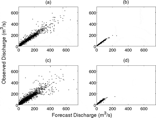
To generate predictive distributions, values of and are used for w_1,j and w_2,j, respectively. When f > 2 and NORA forecasts are being used, all the available time-steps up to the end of 2008 are used; data from 2009 are left for validation purposes. For short lead-times where only observed inputs are used, the dataset from 2004–2008 is split into “forced” and “unforced” time-steps depending upon the presence of effective rainfall input during forecasting steps. Figure 4 shows these have significantly different distributions. In the remainder of this paper, emphasis is placed on the “forced” class, where applicable, since this contains the rising limbs of flood hydrographs which are the time periods of most interest.

Fig. 4 Scatter plots of the observed discharge vs that forecast with lead-times of (a) and (b) 1 h; and (c) and (d) 2 h. For each lead-time, the dataset is separated into forced (left-hand panes) and unforced (right-hand panes) time- steps to show the difference in distribution.

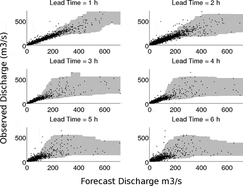
Figure 5 shows a scatter plot of y_t+f against for lead-times of up to 6 h superimposed over a summary of the predictive distributions for differing values of . The derived 95% prediction confidence intervals broadly bracket the data; some outliers can be noted. For example a series of points representing the rising limb of the event hydrograph whose maximum observed discharge is 700 m³/s is poorly forecast at all lead-times. This is due, in part, to inadequacy in the hydrological modelling of the event, which, perhaps due to inadequacies in the observed rainfall input, fails to capture the start of the rising limb until data are assimilated. It could also be due, in part, to observational error in the water-level record for this event which would be amplified by application of the rating curve. Also of note (and witnessed in Table 3) is that the correlation between forecast and observed discharge decreases for higher values at longer lead-times. This results in the derived non-parametric prediction intervals which do not bracket the forecast discharge. This indicates the techniques used attempt to represent not only the magnitude of the forecast residuals but also their bias.

Fig. 7 Forecasts for lead times of up 6 h issued for the largest of the validation events in 2009. The shaded area represents the 95% prediction interval, solid lines the deterministic model forecast and points the observed discharge.

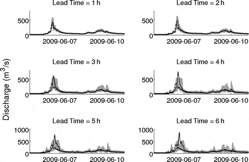
Fig. 5 Scatter plots of against used in the estimation of non-parametric error distribution which is represented by the 95% prediction interval (shaded area) for various forecast lead-times.

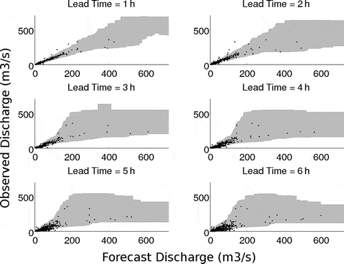
Figure 6 reproduces Fig. 5, but using data for the 13 validation events in 2009. This shows that, for the limited validation data, the prediction error bounds of the forced data seem acceptable. To illustrate the forecasts offered, Fig. 7 shows the forecasts issued with up to 6 h lead-time for the validation event that produces the largest discharge, which is not well characterized by the deterministic hydrological forecast at longer lead-times. At all lead-times, the 95% prediction interval brackets the rising limb and peak of the main event hydrograph. With increasing lead-time, the precision of the forecasts of the hydrograph decreases and is more marked on the falling limb. This may be a result of not separating the “driven” and “non-driven” time-steps for lead-times >2 h. The double peak witnessed in the prediction intervals for the event at 5- and 6-h lead-times is a result of the upper bounds taking a lower value at highest forecast discharges, as can be observed in Fig. 6. This adds further support for the need to separate the “driven” and “non-driven” time-steps if an adequate amount of forecast data are available. It may also suggest the need to include a priori conditions in the derivation of the non-parametric conditional distributions, such as ensuring the bounds are strictly increasing.

Fig. 6 Scatter plots of against for the validation storms in 2009 overlaying the non-parametric error distribution which is represented by the 95% prediction interval (shaded area) for various forecast lead-times.

CONCLUSIONS

The work presented shows a DBM model capable of representing the discharge dynamics in small Alpine basins. The forecasts of the model are improved by the assimilation of observed discharge data to correct a subset of the states of the model. Further observations, for example estimates of stored snow volumes, could be used to refine this model and also allow an additional level of data assimilation. Coupling this model with predictions of future precipitation, such as the NORA forecasts presented, allows discharge forecasts to be issued for longer lead-times.

The performance of the NORA-derived discharge forecasts deteriorates, compared with those produced using the (unknown) future observed precipitation, for lead-times >4 h. A methodology for representing the predictive distribution of the discharge is outlined based on a non-parametric representation of the conditional distributions of transformed data. The results presented suggest that the methodology may be able to adequately represent the forecast uncertainty, particularly when the driven and non-driven time periods are separated. The limited time periods for which NORA forecasts are currently available tempers the conclusions that can be drawn from the forecast performance.

To implement the proposed system in an operational environment, further work would need to be undertaken, both in increasing the catalogue of NORA forecasts and in testing the robustness of the algorithms to missing or corrupted data.

Funding The work reported in this paper has been supported by the EU FP7 project “IMPRINTS”.

REFERENCES

- Alfieri, L., et al., 2011. A staggered approach to flash flood forecasting—case study in the Cévennes region. Advances in Geosciences, 29, 13–20.
- Bàrdossy, A. and Li, J., 2008. Geostatistical interpolation using copulas. Water Resources Research, 44, W07412.
- Beven, K.J., et al., 2005. The uncertainty cascade in flood forecasting. In: P. Balbanis, D. Lambroso, and P. Samuels, eds. Innovation, advances and implementation of flood forecasting technology. Tromsø: ACTIF, abstract, p. 33 , paper 9p on CD (ISBN 978-1-898485-12-4).
- Beven, K.J., Smith, P.J., and Wood, A., 2011. On the colour and spin of epistemic error (and what we might do about it). Hydrology and Earth System Sciences, 15, 3123–3133.
- Bogner, K. and Pappenberger, F., 2011. Multiscale error analysis, correction, and predictive uncertainty estimation in a flood forecasting system. Water Resources Research, 47, W07524.
- Braun, L., 1985. Simulation of snowmelt–runoff in lowland and lower Alpine regions of Switzerland. Zürich: ETH, Zürcher Geographische Schriften, Heft 21 [Available from: Institute for Atmospheric and Climate Science ETH, Winterthurerstr. 190, CH-8057 Zürich].
- Cloke, H.L. and Pappenberger, F., 2009. Ensemble flood forecasting: a review. Journal of Hydrology, 375, 613–626.
- Dietrich, J., et al., 2009. Assessing uncertainties in flood forecasts for decision making: prototype of an operational flood management system integrating ensemble predictions. Natural Hazards and Earth System Sciences, 9, 1529–1540.
- Duband, D., 1970. Reconnaissance dynamique de la forme des situations météorologiques. Application à la prevision quantitative des précipitations. Thesis (PhD), Faculté des Sciences de Paris, France.
- Fan, J. and Gijbels, I., 1996. Local polynomial modelling and its applications. London: Chapman and Hall.
- Germann, U. and Zawadki, I., 2002. Scale dependence of the predictability if precipitation from continental radar images. Part I: Description of the methodology. Monthly Weather Review, 130, 2859–2873.
- Germann, U., Zawadki, I., and Turner, B., 2006a. Predictability of precipitation from continental radar images. Part IV: Limits to prediction. Journal of Atmospheric Sciences, 63, 2092–2108.
- Germann, U., et al., 2006b. Radar precipitation measurement in a mountainous region. Quarterly Journal of the Royal Meteorological Society, 132, 1669–1692.
- Hall, P., Rodney, C.L.W., and Qiwei, Y., 1999. Methods for estimating a conditional distribution. Journal of the American Statistical Association, 94, 154–163.
- Hanson, B.E., 2004. Nonparametric estimation of smooth conditional distributions [online]. University of Wisconsin. Available from: http://www.ssc.wisc.edu/~bhansen/papers/cdf.html [ Accessed 5 April 2013]
- Herr, H.D. and Krzysztofowicz, R., 2010. Bayesian ensemble forecast of river stages and ensemble size requirements. Journal of Hydrology, 387, 151–164.
- Jakeman, A. and Young, P., 1979. Refined instrumental variable methods of recursive time-series analysis. 2. Multivariable systems. International Journal of Control, 29, 621–644.
- Joe, H., 1997. Multivariate models and dependence concepts. London: Chapman and Hall.
- Keef, C., Svensson, C., and Tawn, J. A., 2009. Spatial dependence in extreme river flows and precipitation for Great Britain. Journal of Hydrology, 378, 240–252.
- Kelly, K.S. and Krzysztofowicz, R., 2000. Precipitation uncertainty processor for probabilistic river stage forecasting, Water Resources Research, 36 (9), 2643–2653.
- Krzysztofowicz, R., 1999. Bayesian theory of probabilistic forecasting via deterministic hydrologic model. Water Resources Research, 35, 2739–2750.
- Lees, M.J., et al., 1994. An adaptive flood warning scheme for the River Nith at Dumfries. In: W. Watts and J. Watts, eds. Second international conference on river flood hydraulics. Chichester: John Wiley & Sons Ltd.
- Mandapaka, P.V., et al., 2012. Can Lagrangian extrapolation of radar fields be used for precipitation nowcasting over complex Alpine orography? Weather and Forecasting, 27, 28–49.
- Marsigli, C., et al., 2005. The COSMO-LEPS mesoscale ensemble system: validation of the methodology and verification. Nonlinear Processes in Geophysics, 12, 527–536.
- Marsigli, C., Montani, A., and Paccangnella, T., 2008. A spatial verification method applied to the evaluation of high-resolution ensemble forecasts. Meteorological Applications, 15, 125–143.
- Montanari, A. and Brath, A., 2004. A stochastic approach for assessing the uncertainty of rainfall–runoff simulations. Water Resources Research, 40, W01106.
- Nelson, R.B., 1998. An introduction to copulas. Berlin: Springer-Verlag, Lecture Notes in Statistics 139.
- Obled, C., Bontron, G., and Garcon, R., 2002. Quantitative precipitation forecasts: a statistical adaptation of model outputs through an analogues sorting approach. Atmospheric Research, 63, 303–324.
- Panziera, L. and Germann, U., 2010. The relationship between airflow and orographic precipitation on the southern side of the Alps as revealed by weather radar. Quarterly Journal of the Royal Meteorological Society, 136, 222–238.
- Panziera, L., et al., 2011. NORA—Nowcasting of Orographic Rainfall by means of Analogues. Quarterly Journal of the Royal Meteorological Society, 137, 2106–2123.
- Ranzi, R., Zappa, M., and Bacchi, B., 2007. Hydrological aspects of the Mesoscale Alpine Programme: findings from field experiments and simulations. Quarterly Journal of the Royal Meteorological Society, 133, 867–880.
- Romanowicz, R.J., Young, P.C., and Beven, K.J., 2006. Data assimilation and adaptive forecasting of water levels in the River Severn catchment, United Kingdom. Water Resources Research, 42, W06407.
- Romanowicz, R.J., et al., 2008. A data based mechanistic approach to nonlinear flood routing and adaptive flood level forecasting. Advances in Water Resources, 31, 1048–1056.
- Rossa, A., et al., 2011. The COST 731 Action: a review on uncertainty propagation in advanced hydro-meteorological forecast systems. Atmospheric Research, 100 (2–3),150–167.
- Rotach, M.W., et al., 2009. MAP D-PHASE real-time demonstration of weather forecast quality in the Alpine region. Bulletin of the American Meteorological Society, 90 (9), 1321–1336.
- Salvadori, G. and De Michele, C., 2007. On the use of copulas in hydrology: theory and practice. Journal of Hydrologic Engineering, 12, 369–380.
- Sancetta, A. and Satchell, S., 2004. The Bernstein copula and its applications to modeling and approximations of multivariate distributions. Econometric Theory, 20, 535–562.
- Schaake, J.C., et al., 2007. HEPEX: The hydrological ensemble prediction experiment. Bulletin of the American Meteorological Society, 88, 1541–1547.
- Schweppe, F.C., 1965. Evaluation of likelihood functions for Gaussian signals. IEEE Transactions on Information Theory, 11, 61–70.
- Sirangelo, B., Versace, P., and De Luca, D.L., 2007. Rainfall nowcasting by at site stochastic model PRAISE. Hydrology and Earth System Sciences, 11, 1341–1351.
- Sklar, A., 1959. Fonctions de repartition á n dimensions et leurs marges. Publications de l’Institut de Statistique de l’Univiversite de Paris, 8, 229–231.
- Smith, P.J. and Beven, K.J., 2010. Forecasting river levels during flash floods using data based mechanistic models, online data assimilation and meteorological forecasts. In: Proceedings of the British Hydrological Society international symposium, 1 July 2010, Newcastle. London: British Hydrological Society.
- Smith, P.J., et al., 2008. The provision of site specific flood warnings using wireless sensor networks. In: P. Samuels, S. Huntingdon, W. Allsop, and J. Harrop, eds. Flood risk management: research and practice. Balkema: CRC Press, 212. Abstract, paper on CD. ISBN 978-0-415-48507-4.
- Smith, P.J., et al., 2012. Flash flood forecasting using data based mechanistic models and radar rainfall forecasts. In: R.J. Moore, S.J. Cole, and A.J. Illingworth, eds. Weather radar and hydrology. Wallingford: IAHS Press, IAHS Publ. 351, 562–567.
- Smith, P.J., Beven, K., and Horsburgh, K., 2013. Data based mechanistic modelling of tidally affected river reaches for flood warning purposes: an example on the River Dee, UK. Quarterly Journal of the Royal Meteorological Society, 139 (671), 340–349.
- Song, S. and Singh, V.P., 2010. Frequency analysis of droughts using the Plackett copula and parameter estimation by genetic algorithm. Stochastic Environmental Research and Risk Assessment, 24, 783–805.
- Thielen, J., et al., 2009. Monthly-, medium-, and short-range flood warning: testing the limits of predictability. Meteorological Applications, 16, 77–90.
- Todini, E., 2008. A model conditional processor to assess predictive uncertainty in flood forecasting. International Journal of River Basin Management, 6 (2), 123–137.
- Weerts, A.H., Winsemius, H.C., and Verkade, J.S., 2011. Estimation of predictive hydrological uncertainty using quantile regression: examples from the National Flood Forecasting System (England and Wales). Hydrology and Earth System Sciences, 15, 255–265.
- Wilks, D.S., 1995. Statistical methods in the atmospheric sciences. New York: Academic Press.
- Wöhling, T., Lennartz F., and Zappa, M., 2006. Updating procedure for flood forecasting with conceptual HBV-type models. Hydrology and Earth System Sciences, 10, 783–788.
- Young, P.C., 2001. Data-based mechanistic modelling and validation of rainfall–flow processes. In: M.G. Anderson and P.D. Bates, eds. Model validation: Perspectives in hydrological science. Chichester: John Wiley & Sons Ltd., 117–161.
- Young, P.C., 2002. Advances in real-time flood forecasting. Philosophical Transactions of the Royal Society (A), 360 (1796), 1433–1450.
- Young, P.C., 2003. Top-down and data-based mechanistic modelling of rainfall–flow dynamics at the catchment scale. Hydrological Processes, 17 (11), 2195–2217.
- Young, P.C., 2006. The data-based mechanistic approach to the modelling, forecasting and control of environmental systems. Annual Reviews in Control, 30 (2), 169–182.
- Young, P.C. and Beven, K.J., 1994. Data-based mechanistic modeling and the rainfall–flow nonlinearity. Environmetrics, 5, 335–363.
- Young, P.C., Castelletti, A., and Pianosi, F., 2007. The data-based mechanistic approach in hydrological modelling. In: A. Castelletti and R.S. Sessa, eds. Topics on system analysis and integrated water resource management. Amsterdam: Elsevier, 27–48.
- Young, P.C., Chotai, A., and Beven, K.J., 2004. Data-based mechanistic modelling and the simplification of environmental systems. In: J. Wainwright and M. Mullgan, eds. Environmental modelling: finding simplicity in complexity. Chichester: John Wiley & Sons Ltd., 371–388.
- Young, P. and Jakeman, A., 1979. Refined instrumental variable methods of recursive time-series analysis. 1. Single input, single output systems. International Journal of Control, 29, 1–30.
- Young, P., Jakeman, A., and McMurtrie, R., 1980. An instrumental variable method for model order identification. Automatica, 16, 281–294.
- Young, P.C., McKenna, P., and Bruun, J., 2001. Identification of non-linear stochastic systems by state dependent parameter estimation. International of Journal of Control, 74 (18), 1837–1857.
- Zappa, M., et al., 2008. MAP D-PHASE: real-time demonstration of hydrological ensemble prediction systems. Atmospheric Science Letters, 9 (2), 80–87.
- Zappa, M., et al., 2011. Superposition of three sources of uncertainties in operational flood forecasting chains. Atmospheric Research, 100 (2–3), 246–262.