A non-uniqueness problem in the identification of power-law spectral scaling for hydroclimatic time series

Abstract

Power-law spectral scaling violates assumptions of standard analyses such as statistical change detection. However, hydroclimatic data sets may be too short to differentiate the spectra of 1/f ^α vs low-order linear memory processes, an ambiguity exacerbated by the ubiquity of both process types. We explore this non-uniqueness problem by applying a heuristic tool to four examples from each of four hydroclimatic data types: circulation indices, station climate, river and aquifer conditions, and glacier mass balance. This selection spans much of the globe and includes some of the longest instrumental data sets available. The most common outcome is that power-law scaling is apparent, but the record is insufficiently long to discriminate between underlying mechanisms. The use of palaeoclimatic data to extend the instrumental record was investigated, but produced mixed results. Conversely, a balance-of-evidence approach, additionally incorporating physical process considerations, may help us recognize variate classes for which 1/f ^α scaling can be concluded. Practical recommendations are offered.

Editor D. Koutsoyiannis

Citation Fleming, S.W., 2013. A non-uniqueness problem in the identification of power-law spectral scaling for hydroclimatic time series. Hydrological Sciences Journal, 59 (1), 73–84.

Résumé

La scalance spectrale d’une loi de puissance ne satisfait pas les hypothèses des analyses classiques telles que la détection des changements statistiques. Les ensembles de données hydroclimatiques peuvent cependant être trop courts pour différencier les processus de spectres en 1/fα des processus linéaires à mémoire courte, ambiguïté exacerbée par l’omniprésence de ces deux types de processus. Nous avons exploré ce problème de non-unicité en appliquant un outil heuristique à quatre exemples de chacun de quatre types de données hydro-climatiques suivants: indices de circulation, climat d’une station, caractéristiques d’une rivière et d’un aquifère et bilan de masse d’un glacier. Cette sélection est répartie sur une grande partie du globe et comprend certaines des plus longues séries disponibles de données instrumentales. Le premier résultat est que la scalance selon une loi de puissance est évidente, mais que les séries ne sont pas suffisamment longues pour distinguer entre les mécanismes sous-jacents. L’utilisation des données paléoclimatiques pour étendre la durée des séries instrumentales a été étudiée, mais n’a fourni que des résultats mitigés. Inversement, une approche par bilan des informations, intégrant en outre des considérations de processus physiques, peut nous aider à reconnaître les classes de variables pour lesquelles on peut conclure à une scalance en 1/fα. Des recommandations pratiques sont proposées.Mots clefs spectre ; persistance ; écoulement ; eaux souterraines ; glacier ; paléoclimats

Key words:

• spectrum
• persistence
• streamflow
• groundwater
• glacier
• palaeoclimate

1 INTRODUCTION

Power-law spectral scaling refers to a power-law functional form to the square of the Fourier amplitude spectrum of a time series, in particular, a background spectral density function or periodogram which (apart from peaks corresponding to distinct periodicities) scales as 1/f ^α, where f is frequency and α is a constant. Such dynamics are believed to be widespread in physical, biological and social time series, and have been associated with various statistical or physical generating models. Power-law spectral scaling involves extended system memory, and very closely linked though not necessarily synonymous concepts include long-term persistence (LTP), long-range dependence (LRD), fractal dynamics and the Hurst phenomenon. Intuitively, such behaviour may be interpreted as self-affinity in time, analogous to spatial fractals such as a river drainage network or the branching of a tree: superposition of small, frequent variations upon larger, less frequent or slower variations upon still larger and longer-term variability and so forth (e.g. Kirchner et al. 2001), with repetition of similar dynamical patterns over many different timescales.

Power-law spectral scaling can be important to hydroclimatic investigations for two reasons. The first is fundamental: its ubiquity is such that it appears to be a central feature of nature requiring explanation (e.g. Mandelbrot and Wallis 1969, Press 1978). The second is practical. Power-law spectral scaling and related phenomena have associated effects, such as an elevated tendency to generate runs and clustering, which violate the assumptions of many standard statistical and time-series analysis techniques—in particular, assumptions that samples are uncorrelated (or correlated in a simple way) in time. Potentially strong implications may exist for flood frequency analysis, drought duration assessment, climate data quality-control and homogenization, and long-term trend analysis including climate change signal detection (e.g. Booy and Morgan 1985, Pelletier and Turcotte 1997, Bunde et al. 2005, Cohn and Lins 2005, Rybski et al. 2006, Steirou and Koutsoyiannis 2012). Ability to reproduce low-frequency climate dynamics of this type can also be an important consideration in performance characterization for both mechanistic global climate models and stochastic climate models (e.g. Fleming 2009, Vyushin et al. 2009, Johnson and Sharma 2012).

It is well-established that, broadly speaking, lengthy data sets are needed to properly characterize long-term memory and related effects, and that there can be ambiguities in practice. For instance, in the nonlinear physics literature, Theiler (1991) noted a relationship between spectral scaling, correlation timescale estimates and record length. In statistical hydrology, Khaliq et al. (2009) reported that unambiguous identification of ARFIMA models requires long data sets. As another example, Rakhshandehroo and Amiri (2012) demonstrated that a minimum number of data are required to provide stable estimates of fractal dimension for groundwater level time series. However, it is unclear how thoroughly this question is addressed in many practical water resources or climatology applications, and in particular, rarely does the question of record length specifically arise in empirical identification of power-law scaling from the observational spectra of hydroclimatic data sets. It seems to remain standard practice to conclude 1/f ^α scaling whenever a numerical spectrum estimate appears to suggest it—typically, when a simple linear regression between the logarithms of frequency and power spectral density is statistically significant.

A quite specific, yet potentially very widespread, problem of non-uniqueness with such power spectrum interpretations has recently been identified (Fleming 2008). For short data sets, it may be impossible to reliably differentiate between the complex memory processes which generate genuine power-law spectral scaling vs simple, low-order linear memory (autoregressive) processes which generate quasi-power-law scaling only over a relatively high-frequency band. The lowest observable non-zero frequency in the power spectrum of a finite-duration time series is the Rayleigh frequency, f_Ray, which is inversely proportional to the data set duration, T. For short data sets, f_Ray may be too high to sample the white noise-to-red noise transition which, in practice, serves to distinguish the spectral signature of a low-order linear memory process (which is flat at low f but very nearly 1/f ^α at high f) from that of a “true” 1/f ^α process (which is 1/f ^α over a much wider bandwidth). The problem is deeply compounded by the fact that both types of processes are so common that it is debatable which should be regarded as the default or null hypothesis, and which should be the alternative hypothesis that bears the burden of proof in conventional significance testing (Halley 1996, Cohn and Lins 2005, Fleming 2008). Using a heuristic rule of thumb to assess a couple of long-term observational time series sampling hydroclimatic (among other) systems, Fleming (2008, 2009) demonstrated that these data sets did not meet the criterion for distinguishing between the spectra of short- and long-memory processes. Mistaking a simple autoregressive spectrum for a genuine power-law spectrum could lead to various errors, such as reporting meaningless fractal dimensions or, worse, using incorrect memory adjustment procedures in such socio-economically relevant studies as climate change signal detection analyses. It remains unclear, however, how widespread this type of ambiguity is for hydroclimatic data.

Our aim in this short paper is to better understand the empirical identifiability of 1/f ^α spectral dynamics in hydroclimatic time series, in the light of record length constraints on the uniqueness of long- vs short-memory interpretations of the Fourier spectrum. The approach taken is to apply standard spectral analysis methods, in conjunction with the aforementioned heuristic rule, to unusually long (and thus with respect to 1/f ^α background spectrum detection, best-case scenario) historical records. The 16 instrumental time series considered obviously cannot comprehensively capture all types of hydroclimatic variability, and the technique employed might be best regarded as exploratory in nature. Nevertheless, the careful hydroclimatic data sourcing used—four examples from each of four general data types, with an eye to strong geographic diversity, and employing some of the longest time series of each data type available globally—permits a far clearer view of whether or not ambiguity between the spectra of 1/f ^α and short-memory processes should be an important and widespread practical concern in applied hydroclimatic analysis. We also explore the use of several palaeoclimatic data sets as well as theoretical considerations in evaluating a given hydroclimatic metric of interest for 1/f ^α dynamics, and conclude with some specific recommendations for both researchers and practitioners.

2 DATA

Four broad classes of data were considered in an effort to span a variety of hydroclimatic processes: indices of coherent modes of atmosphere–ocean circulation, station climate data, terrestrial hydrologic data sets and glacier mass balance records. For each category, four examples were in turn selected, generally with an emphasis on geographic diversity to avoid regional biases (see e.g. Huybers and Curry 2006) and obtaining the longest records available so as to provide the best possible chance of being able to uniquely identify the power spectrum form. Some characteristics of the resulting 16 data sets are summarized in Table 1, which also lists data sources and corresponding key literature citations. Additional information with respect to data sourcing is provided in the “Acknowledgements” section of this article.

Table 1 Summary of records used in this study. “Start” and “end” are the first and last years of the time series. Acronyms are as follows. NOAA: US National Oceanic and Atmospheric Administration; JISAO: Joint Institute for the Study of the Atmosphere and Ocean; AHCCD: Adjusted Historical Canadian Climate Data; WSC: Water Survey of Canada; RHBN: Reference Hydrometric Basin Network; INSTAAR: Institute of Arctic and Alpine Research, University of Colorado at Boulder.

Data set	Start	End	Source
Circulation indices—instrumental
Atlantic Multidecadal Oscillation (AMO) Index, DJF mean	1857	2011	NOAA Earth System Research Laboratory
North Atlantic Oscillation (NAO) Index, DJF mean	1951	2011	NOAA Climate Prediction Center
Pacific Decadal Oscillation (PDO) Index, DJF mean	1901	2011	JISAO, University of Washington
Oceanic Niño Index (ONI), DJF mean	1950	2011	NOAA Climate Prediction Center
Circulation indices—palaeoclimatological
Dendrochronologically reconstructed PDO index	1661	1991	NOAA National Climatic Data Center; Biondi et al. (2001)
Dendrochronologically reconstructed PDO index	1700	1979	NOAA National Climatic Data Center; D’Arrigo et al. (2001)
Dendrochronologically reconstructed PDO index	993	1996	NOAA National Climatic Data Center; MacDonald and Case (2005)
PDO index reconstructed from historical documents	1470	1998	NOAA National Climatic Data Center; Shen et al. (2006)
Meteorological station data
Annual mean central England air temperature, UK	1659	2011	UK Met Office (HadCET); Parker et al. (1992), Manley (1974)
Annual total precipitation, Penola Post Office, Australia	1863	2010	Bureau of Meteorology “high-quality climate change datasets”
Annual mean air temperature, Toronto, Canada	1841	2010	Environment Canada 2nd generation AHCCD
Sep-Oct mean sea-level pressure, Madras (Chennai), India	1796	2002	University of East Anglia Climate Research Unit; Allan et al. (2002)
Water resources time series
Nile River annual minimum level, Cairo, Egypt	622	1284	Roda Nilometer: Beran (1994), Toussoun (1925)
Naturalized annual mean flow, Thames River, Kingston, UK	1883	2011	UK National River Flow Archive
Annual maximum daily flow, Bow River, Banff, Canada	1911	2010	Environment Canada/WSC/RHBN; Harvey et al. (1999), Brimley et al. (1999)
Annual mean groundwater elevation, Dalton Holme, UK	1889	2011	British Geological Survey National Groundwater Level Archive
Annual net glacier mass balance measurements
Storglaciären (Kebnekaise, Lapland, Sweden)	1946	2004	INSTAAR: Dyurgerov and Meier (2005)
Tsentralnyj Tuyuksu (Tien Shan, Kazakhstan)	1957	2003	INSTAAR: Dyurgerov and Meier (2005)
South Cascade (Cascade Range, Washington, USA)	1953	2003	INSTAAR: Dyurgerov and Meier (2005)
Echuarren Norte (Central Andes, Chile)	1976	2003	INSTAAR: Dyurgerov and Meier (2005)

Organized modes of atmosphere and/or ocean circulation are a common and effective means of summarizing climatic variability and assessing its effects (e.g. Wang and Schimel 2003). Climate indices are particularly heavily used in hydrology studies, with hundreds if not thousands of examples of such applications to streamflow data in analytical (e.g. Fleming et al. 2006, 2007) or forecasting (e.g. Hamlet et al. 2002, Gobena et al. 2013) contexts, and a growing number of applications to subsurface water resources as well (e.g. Fleming and Quilty 2006, Gurdak et al. 2007). A number of such indices are available. Four leading and well-studied teleconnection patterns were selected to represent both the Atlantic and Pacific basins, and both nominally interannual and interdecadal dominant timescales of variability: the Atlantic Multidecadal Oscillation (AMO) index; the Pacific Decadal Oscillation (PDO) index; the North Atlantic Oscillation (NAO) index and El Niño-Southern Oscillation (ENSO), indexed here by the Oceanic Niño Index (ONI), which is used by the US National Oceanographic and Atmospheric Administration (NOAA) for operational classification of ENSO state. The considerably longer Southern Oscillation Index (SOI) instrumental record was also explored, but gave similar results to the ONI (specifically, little evidence for inverse spectral scaling, as discussed in due course below). In each case, we adopted the common procedure of considering annual December–January–February (DJF) means, capturing interannual variability in wintertime circulation.

Surface climate stations are an obvious indicator of local hydroclimatic conditions. Four data sets were selected on the basis of record length and diversity of both geography and climate parameters. The longest available instrumental climate data set available globally appears to be the central England temperature (CET) time series; annual mean air temperature was analysed here. For the Southern Hemisphere, the longest precipitation time series in the Australian Bureau of Meteorology’s homogenized high-quality climate change database is for Penola Post Office in southeastern Australia; total annual precipitation was considered. For North America, we used the longest temperature time series in Environment Canada’s Adjusted Historical Canadian Climate Database (AHCCD), for Toronto; annual mean temperature was evaluated. Finally, for south Asia, we chose a long sea-level pressure (SLP) data set for Madras (now known as Chennai), India. We used the annual Sep–Oct mean value, as this may serve as an index of summertime all-India rainfall associated with the monsoon (Allan et al. 2002).

It is likely that the leading mechanism whereby hydroclimatic variability influences human society is through its direct impacts on rivers and aquifers. We considered annual time series of annual minimum water level of the Nile River near Cairo, as measured at the Roda Nilometer over the period 622–1284 AD. Broadly speaking, such annual minimum levels speak to seasonal habitat availability and drought. This data set served as the basis for early discoveries by Hurst (1951) and Mandelbrot and Wallis (1969) regarding LTP, and remains in widespread use for such studies today (e.g. Koutsoyiannis 2006). It appears to be the longest hydrometric record available worldwide. Moving on to Northern Europe, the longest instrumental hydrometric record in the United Kingdom is the naturalized flow series for the Thames River at Kingston; we evaluated annual mean flow, an overall measure of water supply availability. For North America, we analysed the longest hydrometric record in Canada amongst those within the Reference Hydrometric Basin Network (RHBN), a subset of Water Survey of Canada streamgauges which has been identified for use in hydroclimate studies; annual maximum daily flow, a measure of habitat disturbance, erosion and flooding potential, was considered for the Bow River at Banff. Finally, we studied annual mean groundwater elevation at Dalton Holme, UK. The well is installed in the shallow Chalk Aquifer, the major groundwater supply in the UK (e.g. Holman et al. 2011). This data set may be the longest record available globally of apparently anthropogenically undisturbed (at least, by local-scale pumping) groundwater levels.

Mountain glaciers are sentinels of climatic variability and change (e.g. Thompson et al. 2008), contribute substantially to sea-level rise as they recede (e.g. Arendt et al. 2002) and affect local-to-mesoscale meteorology, by generating katabatic winds for example (e.g. Söderberg and Parmhed 2006). Of particular interest to us, however, is that they lie at the heart of such continental-scale “water towers” (e.g. Qiu 2010) as the Rocky Mountains, Alps and Himalayas, feeding associated and often transboundary river systems like the Columbia, Athabasca, Danube, Rhine, Indus, Ganges, Brahmaputra, Yangtze and Yellow (Huang He). We consider the longest continuous mountain glacier mass balance records available for each of four continents: Europe (Storglaciären, Sweden); Asia (Tsentralnyj Tuyuksu, Kazakhstan); North America (South Cascade Glacier, USA) and South America (Echuarren Norte, Chile). Annual (net) mass balance, the difference in mm water equivalent between seasonal accumulation and ablation, is a standard measure of the expansion or contraction of glacial ice and was used here. Note that mass balance is in general more directly reflective of climatic conditions than terminus location, which is also heavily influenced by internal glacier physics (e.g. Roe 2011). Note also that glaciers in different climatic regions may show different types of mass balance sensitivity to climate (e.g. maritime vs continental glaciers, Moore et al. 2009; mid- and high-latitude vs tropical glaciers, Mölg et al. 2009). The records from Tsentralnyj Tuyuksu and Echuarren Norte each contained a single, 1-year data gap; these were filled by linear interpolation between values from adjacent years. All the other data sets considered in the study were gap-free.

3 METHODS

Standard methods were used for generating power spectra for each time series and evaluating the results for apparent 1/f ^α scaling. For each data set, x(t), the fast Fourier transform (FFT) algorithm in the R scripting language was used to generate the numerical Fourier transform, X(f). The amplitude spectrum, A(f), was calculated as [Re²(X) + Im²(X)]^1/2. The one-sided power spectral density function (e.g. Press et al. 1992) was in turn generated as PSD(f) = 2A²(f) ∀ 0 ≤ f ≤ f_Nyq, where f_Nyq is the Nyquist frequency, (2Δt)^-1, and Δt is the sampling frequency, equal to 1 year in all the cases considered here. The existence of a relationship between ln(f) and ln(PSD) was then evaluated using methods typically employed for this purpose: specifically, a significance test on the Pearson correlation coefficient to generate p values under the standard assumptions of linearity and an IID (independent and identically distributed) normal distribution; similarly, α was estimated by standard linear least-squares regression from ln(PSD) = β₀ + β₁ln(f) with α = –β₁. The full non-zero frequency range sampled by a given observational time series was used in this evaluation of linear association, extending from the Rayleigh frequency, f_Ray = T ^-1 = (NΔt)^-1 where N is the number of samples, through to the Nyquist frequency.

We then assessed, in the case of apparent power-law spectral scaling (i.e. in the case that ln(PSD) is found to be a linear function of ln(f) at p ≤ ~0.05), whether the records are in fact sufficiently long to discriminate between low-order linear memory vs a power-law spectrum-generating process. This is accomplished using a simple heuristic rule introduced by Fleming (2008):

where ρ is the estimated lag-1 serial correlation coefficient of x(t), estimated simply as the linear correlation coefficient between the yearly data set and a lagged copy of itself; δ is a constant, taken to be 10^-30; and τ* is a critical timescale. A corresponding critical frequency, f * = 1/τ*, is defined as the frequency at which the spectrum of an AR(1) process with parameter ρ begins to transition from a white-noise signature (a flat spectrum in the mean) to a red-noise signature (an inverse frequency-scaled spectrum in the mean). The requirement for discriminating between low-order memory and a power-law generating process is f * >> f_Ray, or equivalently, τ* << T. If on the other hand f * is similar to or lower than f_Ray, or equivalently, τ* is similar to or greater than T, then the data set is insufficiently long to make the distinction. That is, the power spectrum of a low-order linear memory process contains a “break” between red-noise and white-noise signatures, not seen in a power-law process, and the frequency at which this break occurs corresponds to the longest timescale at which memory operates. The foregoing rule of thumb provides an estimate of that critical timescale. It is therefore a means to determine whether the Rayleigh frequency, which is inversely proportional to the data set length, is sufficiently low to effectively capture the red–white spectral transition should it occur. Thus, if the spectrum appears to scale as a power law because a statistically significant association exists between ln(PSD) and ln(f), but the record is not long enough for its Rayleigh frequency to lie well below the critical frequency, then conclusive determinations cannot be made as to the nature of the process: we only can surmise that it involves some kind of red noise. On the other hand, if the spectrum appears to scale as a power law and the record is indeed sufficiently long to sample frequencies well below the critical frequency, then a power-law process can be far more robustly concluded.

In the interest of conciseness, readers are referred to Fleming (2008) for further details on the development and application of this heuristic rule, including the results of extensive testing on synthetic and observational data sets. Nevertheless, some points of application are briefly noted here. (a) A design goal for this rule of thumb was operational simplicity—it is intended largely for scoping analyses, and that is how it is employed here. The results must be interpreted in that light. (b) It may be tempting to address the issue instead by changing the null hypothesis, H₀, in conventional null-hypothesis significance testing (NHST) of ln(f) vs ln(PSD) for linear behaviour, from a white-noise spectrum to an AR(1) spectrum. This is insufficient. Such an approach would not directly answer the question at hand (whether the record is sufficiently long to discriminate between the spectra of short- vs long-memory processes), without making assumptions regarding which of these two red-noise hypotheses must bear the burden of proof as the alternative hypothesis in NHST. This is problematic when both are likely (see Section 1, and Fleming, 2008). (c) The relationships between our analysis and some standard (e.g. Kanasewich 1981, Press et al. 1992, Chatfield 1996, von Storch and Zwiers 1999, Fleming et al. 2002) data pre- and post-processing steps in spectral analysis may be somewhat complicated. We adopt the common procedure of removing the mean prior to analysis. However, periodogram smoothers (e.g. Daniell estimators) are not employed because smearing of spectral power across bands seems counterproductive if one aim is to compare spectral form on either side of a particular threshold, f *. Tapering was also not used, as it causes progressive loss of information near the start and end of the window (in a climatological application, the record start and end). Doing so in effect reduces record length, which seems counterproductive when interest lies with long-period components, and T is small. The typical step of linearly detrending data prior to spectral analysis poses a possible conundrum: 1/f ^α scaling tends to generate local-in-time monotonic trends (Press 1978; see also Matalas and Sankarasubramanian 2003, Cohn and Lins 2005, Koutsoyiannis 2006, Rybski et al. 2006, Khaliq et al. 2009), so detrending may remove the expression of a 1/f ^α process, potentially biasing the result towards concluding that power-law scaling is not present. Conversely, if a structural trend is present, failure to detrend the series might inflate the ρ estimate (e.g. Yue et al. 2002), thus increasing τ* and potentially biasing the result towards concluding insufficient record length to unambiguously identify 1/f ^α dynamics. Our main analysis adopts a standard linear detrending procedure, regressing the hydroclimatic metric on time and removing the resulting best-fit line. To assess sensitivity, however, we performed a re-analysis without detrending; the results (not illustrated here in the interest of conciseness) differed in detail, but the overall outcome was similar. (d) We follow typical statistical hydroclimatology practice by considering annual metrics. Such yearly time series focus the analysis on particular quantities of interest, restrict the analysis to the desired climatological timescales and may in many cases be the finest temporal discretization for which a certain metric of interest is available or physically meaningful. A sub-annual sampling interval would increase N but not T, and would therefore appear to offer little benefit to assessing long-term hydroclimatic dynamics.

4 RESULTS AND DISCUSSION

Three general outcomes are possible for a given time series:

1. It is unlikely that the spectrum follows a genuine power-law form. This may in turn occur for two different reasons:

   1. The first is that the significance test on the correlation coefficient provides no evidence for a statistically significant (p ≤ ~0.05) negative linear association between ln(f) and ln(PSD). That is, there is little evidence for any type of red noise.

   2. The second reason is that such an inverse ln(f)–ln(PSD) relationship appears present based solely on the significance of the correlation coefficient, but this relationship appears to fail over f ≤ f *. That is, red noise is present, but the time series is sufficiently long to differentiate between short- and long-memory alternatives, and the spectral scaling appears to be associated with a low-order linear memory process.

2. A power-law spectrum is possible, but there are insufficient data to tell. In this case, there is a statistically significant relationship between ln(f) and ln(PSD) which appears to hold over the full bandwidth sampled, but τ* is similar to or longer than T. That is, the data set is too short for us to robustly determine whether the reddened spectrum observed is due to a low-order linear memory process or a power-law process.

3. The balance of evidence suggests that the observational data set was generated by a power-law spectrum process. This occurs when all the following conditions appear to be met:

   1. τ* << T;

   2. there is a statistically significant relationship between ln(f) and ln(PSD); and

   3. this relationship holds over all f_Ray ≤ f ≤ f_Nyq.

Before moving on to the results, two brief remarks about what effectively constitutes “true” power-law spectral scaling may be helpful. First, it is impossible for a process to exhibit 1/f ^α scaling ∀ f because of mathematical discontinuities as f → 0 and f → ∞, though in practice these restrictions can be extremely liberal (for a discussion, see Milotti 2002 and references therein). Second, if we are lucky enough to have a very long data set sampling frequencies far below f *, it is perhaps not necessary for a negative linear relationship between ln(f) and ln(PSD) to hold over all f_Ray ≤ f ≤ f * in order to claim power-law spectral scaling. Rather, as discussed in Fleming (2008), for example, it may be sufficient for many practical purposes to identify the process as exhibiting power-law scaling if 1/f ^α behaviour is observed over several orders of magnitude below f *, clearly distinguishing it from a low-order linear memory process. This issue could be important if outcome (1b) arises. Note, however, that while we encountered case (1b) as described below, for none of the particular data sets considered here did we see power-law spectral scaling which persisted over several orders of magnitude below f * only to fail at the very lowest frequencies.

Evaluations were made on a data set-by-data set basis. Each assessment was based on visual examination of the power spectral density function in the light of the corresponding quantitative critical frequency (f *) estimate, and applying a certain degree of qualitative professional judgement. Figure 1 provides some illustrative examples of the empirical power spectra and their critical frequencies, spanning the various data classes and the different outcomes obtained. The overall results of the analyses are compactly summarized in Table 2.

Fig. 1 Illustrative examples of numerical power spectra. Thin, solid, dark grey line gives best-fit regression between ln(f) vs ln(PSD); thick, dashed, light grey vertical line is ln(f *). (a) PDO index (circulation pattern, outcome 2). (b) Central England mean temperature (climate station, outcome 3). (c) Bow River maximum flow (water resources, outcome 1a) (f * undefined and not shown; see Table 2). (d) Storglaciären net balance (glacier mass balance, outcome 2).

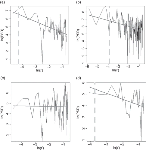
Table 2 Analysis results. “Log regression” gives regression slope, β₁, and significance of correlation, p, corresponding to potential linear associations between ln(f) vs ln(PSD) for each time series. “Heuristic rule” gives data set duration, T; observed serial correlation coefficient of the observational time series, ρ; critical timescale from heuristic rule, τ*; natural logarithm of Rayleigh frequency corresponding to T, ln(f_Ray); and logarithm of frequency corresponding to τ*, ln(f *). “Outcome” summarizes the assessment of background spectrum form for each time series, using both quantitative information and visual spectrum assessments; the numbers correspond to the numbered outcomes discussed in the text.

Data set	Log regression		Heuristic rule					Outcome
	β1	p	T	ρ	τ*	ln(fRay)	ln(f *)
Instrumental climate indices
AMO index	–0.71	<0.01	155	0.61	141	–5.0	–5.0	Possible but insufficient data (2)
NAO index	–0.65	<0.01	61	0.35	67	–4.1	–4.2	Possible but insufficient data (2)
PDO index	–0.70	<0.01	111	0.39	73	–4.7	–4.3	Possible but insufficient data (2)
ONI	0.23	>0.10	62	–0.13	n/a	–4.1	n/a	Unlikely (1a)
Pre-instrumental PDO indices
Biondi et al. (2001)	–1.71	<0.01	331	0.85	414	–5.8	–6.0	Unlikely (1b)
D’Arrigo et al. (2001)	–0.46	<0.01	280	0.37	69	–5.6	–4.2	Possible but insufficient data (2)
MacDonald and Case (2005)	–1.19	<0.01	1004	0.75	236	–6.9	–5.5	Strong evidence (3)
Shen et al. (2006)	–0.16	0.05	529	0.14	35	–6.3	–3.6	Moderate evidence (3)
Station data
Central England temperature	–0.40	<0.01	353	0.24	49	–5.9	–3.9	Strong evidence (3)
SW Australia precipitation	–0.17	>0.10	148	–0.01	n/a	–5.0	n/a	Unlikely (1a)
Eastern Canada temperature	–0.31	0.03	170	0.20	43	–5.1	–3.8	Possible but insufficient data (2)
SE India sea-level pressure	–0.22	>0.10	207	0.16	38	–5.3	–3.6	Unlikely (1a)
Water resources
Nile annual minimum level	–0.67	<0.01	663	0.54	114	–6.5	–4.7	Strong evidence (3)
Thames annual mean flow	–0.35	0.07	129	0.25	50	–4.9	–3.9	Possible but insufficient data (2)
Bow annual maximum flow	–0.03	>0.10	101	–0.12	n/a	–4.6	n/a	Unlikely (1a)
Dalton Holme groundwater level	–0.49	<0.01	123	0.25	50	–4.8	–3.9	Possible but insufficient data (2)
Glacier mass balance
Storglaciären	–0.52	0.03	59	0.19	41	–4.1	–3.7	Possible but insufficient data (2)
Tsentralnyj Tuyuksu	–0.46	>0.10	47	0.26	51	–3.9	–3.9	Possible but insufficient data (2)
South Cascade	0.43	0.04	51	–0.19	n/a	–3.9	n/a	Unlikely (1a)
Echuarren Norte	0.16	>0.10	28	–0.30	n/a	–3.3	n/a	Unlikely (1a)

Note: n/a denotes sample lag-1serial correlation coefficient is (at least nominally) negative, so that τ* and f * are undefined.

Of the 16 instrumental time series explored, six are inferred to be unlikely to demonstrate power-law scaling of the Fourier spectrum; eight remain candidates but have record lengths insufficient to discriminate between short-memory and long-memory interpretations; and two provide solid evidence for a power-law spectral density function as distinct from a low-order linear memory process (Table 2). It is challenging to draw any reliable generalizations, on the basis of this analysis alone, regarding which classes of hydroclimatic variables do or do not fundamentally possess power-law spectra. This is because the results—that is, whether outcome 1a, 1b, 2 or 3 was found for a given data set—simply reflect, in large part, how long that observational record happens to be. Indeed, our main conclusion is that the most common outcome for more than a dozen of the world’s longest instrumental hydroclimatic data sets was that the time series is simply too short to adequately judge the matter.

An obvious response is to examine palaeoclimatic records. This proposed solution is by no means novel. Henley et al. (2011), for example, found that historical observations of precipitation in Australia were too short to permit selection between competing stochastic models, and turned to palaeoclimatic data to complement the instrumental record. Similarly, Markonis and Koutsoyiannis (2013) extended their analyses of LTP in historical temperature data sets by additionally considering a number of very lengthy, proxy-based pre-instrumental records. We explored this option for a widely relevant climatic parameter, the PDO index. This metric (see Table 2 and Fig. 1(a)) clearly exhibits 1/f ^α scaling, but the instrumental record was found to be too short to properly assess the 1/f ^α dynamics. Four independent palaeoclimatic reconstructions of the PDO were considered. Three were based on dendrochronology, using tree rings from various western North American sites, which differed between studies. The fourth PDO index reconstruction utilized historical Chinese documents which classified drought/flood conditions into discrete categories. As for the instrumental records, some characteristics of these data sets are summarized in Table 1, which also lists data sources and corresponding key literature citations.

Outcomes are mixed. The multi-centennial (see Table 1) Biondi et al. (2001) reconstruction showed statistically significant 1/f ^α scaling overall, yet remained insufficiently long to rigorously assess presence of fractal dynamics. More importantly, the linearly decreasing relationship between ln(f) and ln(PSD) appears to fail at low f. This data set therefore argues against true 1/f ^α scaling in the PDO. The D’Arrigo et al. (2001) reconstruction, of roughly similar length, shows a highly significant (p << 0.01) relationship between ln(f) and ln(PSD) which holds over all f_Ray ≤ f ≤ f_Nyq, but the data set does not appear sufficiently long to unambiguously distinguish between short- and long-memory processes. The approximately millennial-scale Macdonald and Case (2005) reconstruction shows clear 1/f ^α scaling over the full frequency range sampled by the data set, and that bandwidth indeed appears sufficient, albeit marginally, to make the distinction between low-order linear memory and power-law spectral dynamics. Overall, the Macdonald and Case (2005) data set yields fairly strong spectral evidence for LTP in the PDO. Finally, the Shen et al. (2006) reconstruction provides modest evidence for true 1/f ^α scaling in the PDO: the data set appears sufficiently long to make the determination, but the relationship between ln(f) and ln(PSD) is somewhat marginal, being significant only at just over p = 0.05. It therefore appears we may have replaced one problem with another: some palaeoclimatic reconstructions are apparently capable of pushing the PDO index record far enough back in time to distinguish between low-order linear memory and power-law spectral dynamics, but the reliability of the resulting Fourier spectra appears insufficient to make those distinctions, given that each of the four PDO reconstructions yields a different answer.

For the PDO, however, we can perhaps adopt a balance-of-evidence approach to assess for power-law scaling, in which we pursue various distinct lines of investigation and consider the results collectively. Empirically, we see that the instrumental record suggests a 1/f ^α spectrum, though being too short to uniquely identify it; three of four palaeoclimatic reconstructions also suggest a 1/f ^α spectrum; and two of four palaeoclimatic reconstructions suggest a 1/f ^α spectrum and are also sufficiently long to differentiate between true power-law scaling and a low-order linear memory process. We can additionally bring theoretical considerations to bear. Very different process modelling approaches have each suggested that the PDO specifically, or ocean temperature in general (note the PDO is a feature of North Pacific sea surface temperature), show a fundamental 1/f ^α spectrum (Fraedrich et al. 2003, Huybers and Curry 2006, Newman 2007). On balance, then, it seems reasonable to conclude that the PDO likely has a true power-law spectrum. An important addendum is that, for the PDO, we have the luxury of multiple independent palaeo-reconstructions and multiple process models of the same quantity, so we can compare 1/f ^α assessment results between them and identify consistencies and inconsistencies. In contrast, one might therefore wonder whether, for palaeoclimatic data sets of which only one version is available, how much confidence can be placed in the corresponding evaluation of spectral form.

5 CONCLUSIONS AND RECOMMENDATIONS

Our analysis of over a dozen of the world’s longest instrumental hydroclimatic records, in combination with broader uncertainties around whether short-term memory or LTP should form the default null hypothesis, confirms that in many cases the observational record is likely too short to either verify or rule out true 1/f ^α spectral behaviour. We also found that extending the record using palaeoclimatic methods was less informative than might be hoped. It is important to note that the contribution of this work is not to identify short- vs long-term persistence as being the dominant process in hydroclimate, but instead to underline and better understand an important point of uncertainty around spectral form, with potential implications to a wide variety of hydroclimatic analyses. Considered collectively, and given that physically-based process models for 1/f ^α spectral dynamics in hydroclimatic systems are thus far somewhat limited, our results suggest that for any given data set, there will often be little a priori guidance or site-specific empirical evidence for which memory model should be assumed.

This finding in turn suggests three recommendations:

1. The missing a priori guidance must be developed, through a deeper and broader understanding of which physical processes lead to power-law spectral scaling, and which do not. If one has broader empirical and/or physical justifications for assuming a particular memory model for a given type of hydroclimatic process, one is freed at least in part from a complete reliance upon local, very long instrumental records to make the determination. For example, in our PDO analyses using both instrumental and pre-instrumental proxy records, we saw how a balance-of-evidence approach additionally incorporating findings from the process modelling community can support empirical assessments of 1/f ^α scaling. Similarly, some physical controls and basis have been explicitly established for LTP in river flow by, for example, Mudelsee (2007) and Szolgayová et al. (2012). Emphasis in that work was not strictly on spectral analysis of annual time series for very long-term hydroclimatic effects, and it remains unclear whether power-law scaling occurs for all streamflow metrics (see e.g. Table 2). Nevertheless, such knowledge should help inform analysts of the conditions under which power-law spectra may appear in river hydrology, and points the direction for additional future research.

2. If the correct spectral form cannot be uniquely identified on the basis of historical records for a given project using the methods outlined in this study, or on the basis of physical considerations as discussed immediately above, then analyses (of trend, climate station homogeneity, drought duration, etc.) should be repeated using all plausible memory interpretations. The results might form the basis for bracketing estimates (cf. Fleming 2007, Vyushin et al. 2009), multiple working models (Overland et al. 2006, Fleming 2009), or strength-of-evidence assessments (Franzke 2012).

3. More accurately capturing frequency-domain behaviour in palaeoclimatic reconstructions is key for some applications, including reliable identification of the background spectrum. We found that four independent palaeoclimatic extensions of a given historical record each gave a different result in terms of identifying power-law spectral dynamics. Perhaps one avenue for further exploration might be to explicitly incorporate replication of spectral form into the model-fitting and validation techniques (e.g. frequency-domain calibration and testingl; Duffy and Gelhar 1985, Fleming et al. 2002) used to generate a hydroclimatic reconstruction from a tree-ring chronology or other palaeo-environmental proxy.

Acknowledgements

The author is deeply indebted to those who helped source the diverse data sets analysed, including Jamie Hannaford (UK National River Flow Archive), Rosemary Fry (British Geological Survey) and Valentina Radic (University of British Columbia). Additionally, Lynne Campo (Meteorological Service of Canada), Sabrina Wong (Environment Canada) and Rosanne D’Arrigo (Columbia University) provided valuable support or advice with respect to selecting and obtaining data sets. These results were presented at the April 2012 European Geosciences Union General Assembly and the June 2012 Canadian Association of Physicists Annual Congress, and the manuscript benefitted significantly from interactions with fellow participants, including, in particular, Elena Szolgayová (TU Vienna), Christian Franzke (British Antarctic Survey), Dan Rosbjerg (Technical University of Denmark), Eva Steirou (National Technical University of Athens), James Kirchner (ETH Zurich/University of California, Berkeley), Kerstin Stahl (University of Freiburg) and Jörn Davidsen (University of Calgary).

REFERENCES

- Allan, R.J., et al., 2002. A reconstruction of Madras (Chennai) mean sea-level pressure using instrumental records from the late 18th and early 19th centuries. International Journal of Climatology, 22, 1119–1142.
- Arendt, A.A., et al., 2002. Rapid wastage of Alaska glaciers and their contribution to rising sea level. Science, 297, 382–386.
- Beran, J., 1994. Statistics for long-memory processes, Monographs on statistics and applied probability. Vol. 61. New York: Chapman and Hall.
- Biondi, F., Gershunov, A,. and Cayan, D.R., 2001. North Pacific decadal climate variability since 1661. Journal of Climate, 14, 5–10.
- Booy, C. & Morgan, D.R., 1985. The effect of clustering of flood peaks on a flood risk analysis for the Red River. Canadian Journal of Civil Engineering, 21, 150–165.
- Brimley, B., et al., 1999. Establishment of the reference hydrometric basin network (RHBN) for Canada. Ottawa: Environment Canada, Internal Report.
- Bunde, A., et al., 2005. Long-term memory: A natural mechanism for the clustering of extreme events and anomalous residual times in climate records. Physical Review Letters, 94, 048701.
- Chatfield, C., 1996. The analysis of time series. 5th ed. London: Chapman and Hall.
- Cohn, T.A. & Lins, H.F., 2005. Nature’s style: Naturally trendy. Geophysical Research Letters, 32. doi:10.1029/2005GL024476
- D’Arrigo, R., Villalba, R., and Wiles, G., 2001. Tree-ring estimates of Pacific decadal climate variability. Climate Dynamics, 18, 219–224.
- Duffy, C.J. and Gelhar, L.W., 1985. A frequency domain approach to water quality modeling in groundwater: Theory. Water Resources Research, 21, 1175–1184.
- Dyurgerov, M.B. and Meier, M.F., 2005. Glaciers and the changing earth system: A 2004 snapshot. University of Colorado, Boulder, CO: Institute of Arctic and Alpine Research, INSTAAR Occasional Paper no. 58.
- Fleming, S.W., 2007. Climatic influences on Markovian transition matrices for Vancouver daily rainfall occurrence. Atmosphere-Ocean, 45, 163–171.
- Fleming, S.W., 2008. Approximate record length constraints for experimental identification of dynamical fractals. Annalen der Physik, 17, 955–969.
- Fleming, S.W., 2009. Exploring the nature of Pacific climate variability using a “toy” nonlinear stochastic model. Canadian Journal of Physics, 87, 1127–1131.
- Fleming, S.W., et al., 2002. Practical applications of spectral analysis to hydrologic time series. Hydrological Processes, 16, 565–574. See also erratum: Fleming, S.W., et al., 2003, Hydrological Processes, 17, 883.
- Fleming, S.W., et al., 2007. Regime-dependent streamflow sensitivities to Pacific climate modes across the Georgia-Puget transboundary ecoregion. Hydrological Processes, 21, 3264–3287.
- Fleming, S.W., Moore, R.D., and Clarke, G.K.C., 2006. Glacier-mediated streamflow teleconnections to the Arctic Oscillation. International Journal of Climatology, 26, 619–636.
- Fleming, S.W., and Quilty, E.J., 2006. Aquifer responses to El Niño-Southern Oscillation, southwest British Columbia. Ground Water, 44, 595–599.
- Fraedrich, K., Luksch, U., and Blender, R., 2003. 1/f model for long-time memory of the ocean surface temperature. Physical Review E, 70, 037301.
- Franzke, C., 2012. Nonlinear trends, long-range dependence and climate noise properties of surface temperature. Journal of Climate, 25 (12), 4172–4183. doi:10.1175/JCLI-D-11-00293.1
- Gobena, A.K., Weber, F.A., and Fleming, S.W., 2013. The role of large-scale climate modes in regional streamflow variability and implications for water supply forecasting: A case study of the Canadian Columbia River Basin. Atmosphere-Ocean, 51 (4), 380–391. doi:10.1080/07055900.2012.759899
- Gurdak, J.J., et al., 2007. Climate variability controls on unsaturated water and chemical movement, High Plains Aquifer, USA. Vadose Zone Journal, 6, 533–547. doi:10.2136/vzj2006.0087
- Halley, J.M., 1996. Ecology, evolution, and 1/f-noise. Trends in Ecology and Evolution, 11, 33–37.
- Hamlet, A.F., Huppert, D., and Lettenmaier, D.P., 2002. Economic value of long-lead streamflow forecasts for Columbia River hydropower. ASCE Journal of Water Resources Planning and Management, 128, 91–101.
- Harvey, K.D., Pilon, P.J., and Yuzyk, T.R., 1999. Canada’s reference hydrometric basin network (RHBN). In CWRA 51st annual conference. Halifax: Canadian Water Resources Association.
- Henley, B.J., et al., 2011. Climate-informed stochastic hydrological modeling: Incorporating decadal-scale variability using paleo data. Water Resources Research, 47. doi:10.1029/2010WR010034
- Holman, I.P., et al., 2011. Identifying non-stationary groundwater level response to North Atlantic ocean–atmosphere teleconnection patterns using wavelet coherence. Hydrogeology Journal. doi 10.1007/s10040-011-0755–9
- Hurst, H.E., 1951. Long-term storage capacity of reservoirs. Transactions of the American Society of Civil Engineers, 116, 770–799.
- Huybers, P. and Curry, W., 2006. Links between annual, Milankovitch and continuum temperature variability. Nature. doi:10.1038/nature04745
- Johnson, F., and Sharma, A., 2012. On long-term persistence in GCM rainfall simulations: Implications for water resources planning and design. Geophysical Research Abstracts, 14, EGU2012-4731.
- Kanasewich, E.R., 1981. Time sequence analysis in geophysics. 3rd ed. Edmonton: University of Alberta Press.
- Khaliq, M.N., Ouarda, T.B.M.J., and Gachon, P., 2009. Identification of temporal trends in annual and seasonal low flows occurring in Canadian rivers: the effect of short- and long-term persistence. Journal of Hydrology, 369, 183–197.
- Kirchner, J.W., Feng, X., and Neal, C., 2001. Catchment-scale advection and dispersion as a mechanism for fractal scaling in stream tracer concentrations. Journal of Hydrology, 254, 82–101.
- Koutsoyiannis, D., 2006. Nonstationarity versus scaling in hydrology. Journal of Hydrology, 324, 239–254.
- MacDonald, G.M., and Case, R.A., 2005. Variations in the Pacific Decadal Oscillation over the past millennium. Geophysical Research Letters, 32. doi:10.1029/2005GL022478
- Mandelbrot, B.B., and Wallis, J.R., 1969. Some long-run properties of geophysical records. Water Resources Research, 5, 321–340.
- Manley, G., 1974. Central England temperatures: Monthly means 1659–1973. Quarterly Journal of the Royal Meteorological Society, 100, 389–405.
- Markonis, Y., and Koutsoyiannis, D., 2013. Climatic variability over time scales spanning nine orders of magnitude: connecting Milankovitch cycles with Hurst-Kolmogorov dynamics. Surveys in Geophysics, 34, 181–207.
- Matalas, N.C., and Sankarasubramanian, A., 2003. Effect of persistence on trend detection via regression. Water Resources Research, 39. doi:10.1029/2003WR002292
- Milotti, E., 2002. 1/f Noise: A Pedagogical Review. arXiv:physics/0204033v1 [physics.class-ph].
- Moore, R.D., et al., 2009. Glacier change in western North America: Influences on hydrology, geomorphic hazards, and water quality. Hydrological Processes, 23, 42–61.
- Mölg, T., Cullen, N.J., and Kaser, G., 2009. Solar radiation, cloudiness and longwave radiation over low-latitude glaciers: Implications for mass-balance modelling. Journal of Glaciology, 55, 292–302.
- Mudelsee, M., 2007. Long memory of rivers from spatial aggregation. Water Resources Research, 43. doi:10.1029/2006WR005721
- Newman, M., 2007. Interannual to decadal predictability of tropical and north Pacific sea surface temperatures. Journal of Climate, 20, 2333–2356.
- Overland, J.E., Percival, D.B., and Mofjeld, H.O., 2006. Regime shifts and red noise in the North Pacific. Deep-Sea Research, 53, 582–588.
- Parker, D.E., Legg, T.P., and Folland, C.K., 1992. A new daily central England temperature series, 1772–1991. International Journal of Climatology, 12, 317–342.
- Pelletier, J.D., and Turcotte, D.L., 1997. Long-range persistence in climatological and hydrological time series: analysis, modeling and application to drought hazard assessment. Journal of Hydrology, 203, 198–208.
- Press, W.H., 1978. Flicker noises in astronomy and elsewhere. Comments on Astrophysics, 7, 103–119.
- Press, W.H., et al., 1992. Numerical recipes in Fortran 77. 2nd ed. Cambridge: Cambridge University Press.
- Qiu, J., 2010. Measuring the meltdown. Nature, 468, 141–142.
- Rakhshandehroo, G.R. and Amiri, S.M., 2012. Evaluating fractal behavior in groundwater level fluctuations time series. Journal of Hydrology, 464–465, 550–556.
- Roe, G.H., 2011. What do glaciers tell us about climate variability and climate change? Journal of Glaciology, 57, 567–578.
- Rybski, D., et al., 2006. Long-term persistence in climate and the detection problem. Geophysical Research Letters, 33. doi:10.1029/2005GL025591
- Shen, C., et al., 2006. A Pacific Decadal Oscillation record since 1470 AD reconstructed from proxy data of summer rainfall over eastern China. Geophysical Research Letters, 33. doi:10.1029/2005GL024804
- Söderberg, S., and Parmhed, O., 2006. Numerical modelling of katabatic flow over a melting outflow glacier. Boundary-Layer Meteorology, 120, 509–534.
- Steirou, E., and Koutsoyiannis, D., 2012. Investigation of methods for hydroclimatic data homogenization. Geophysical Research Abstracts, 14, EGU2012-956-1
- Szolgayová, E., Blöschl, G., and Bucher, C., 2012. Factors influencing long range dependence in streamflow of European rivers. Geophysical Research Abstracts, 14, EGU2012-10776
- Theiler, J., 1991. Some comments on the correlation dimension of 1/f α noise. Physics Letters A, 155, 480–493.
- Thompson, L.G., et al., 2008. Tibetan glaciers as integrators and sentinels of climate change. Abstract #GC11B-07. American Geophysical Union Fall Meeting, San Francisco, CA.
- Toussoun, O., 1925. Chapitre XI: Les Niveaux, Tome Deuxiéme: Memoire sur l’Histoire du Nil. In: Memoires à L’Institut D’Egypte. Cairo: Imprimerie de l’Institut Français d’Archéologie Orientale, 366–392.
- von Storch, H., and Zwiers, F.W., 1999. Statistical analysis in climate research. Cambridge: Cambridge University Press.
- Vyushin, D.I., Kushner, P.J., and Mayer, J., 2009. On the origins of temporal power-law behavior in the global atmospheric circulation. Geophysical Research Letters, 36. doi:10.1029/2009GL038771
- Wang, G., and Schimel, D., 2003. Climate change, climate modes, and climate impacts. Annual Review of Environment and Resources, 28, 1–28.
- Yue, S., et al., 2002. The influence of autocorrelation on the ability to detect trend in hydrological series. Hydrological Processes, 16, 1807–1829.